ESAIM: PS 24 (2020) 718–738 ESAIM: Probability and Statisticshttps://doi.org/10.1051/ps/2020025 www.esaim-ps.org

CHAIN-REFERRAL SAMPLING ON STOCHASTIC BLOCK

MODELS∗

Thi Phuong Thuy Vo∗∗

Abstract. The discovery of the “hidden population”, whose size and membership are unknown, ismade possible by assuming that its members are connected in a social network by their relationships.We explore these groups by a chain-referral sampling (CRS) method, where participants recommend thepeople they know. This leads to the study of a Markov chain on a random graph where vertices representindividuals and edges connecting any two nodes describe the relationships between correspondingpeople. We are interested in the study of CRS process on the stochastic block model (SBM), whichextends the well-known Erdos-Renyi graphs to populations partitioned into communities. The SBMconsidered here is characterized by a number of vertices N , a number of communities (blocks) m,proportion of each community π = (π1, . . . , πm) and a pattern for connection between blocks P =(λkl/N)(k,l)∈{1,...,m}2 . In this paper, we give a precise description of the dynamic of CRS process indiscrete time on an SBM. The difficulty lies in handling the heterogeneity of the graph. We prove thatwhen the population’s size is large, the normalized stochastic process of the referral chain behaves likea deterministic curve which is the unique solution of a system of ODEs.

Mathematics Subject Classification. 05C80, 60J05, 60F17, 90B15, 92D30, 91D30.

Received June 9, 2019. Accepted September 18, 2020.

1. Introduction

In sociology, some populations may be hidden because their members share common attributes that areillegal or stigmatized. These hidden groups may be hard to approach because these individuals try to concealtheir identities due to legal authorities (e.g. drugs users) or because of the social pressure (e.g. men havingsex with men). In such populations, all the information is unknown: there is no sampling frame such as listsof the members of the population or of the relationship between the latter. It causes many challenges forresearchers to identify these groups. The discovery of the hidden populations is made possible by assumingthat its members are connected by a social network. The population is described by a graph (network) whereeach individual is represented by a vertex and any interaction or relationship (e.g. friendship, partnership)between a couple of individuals is represented by an edge matching the corresponding vertices. Thanks to this

∗This work was done during the Ph.D. thesis of the author under the supervision of Jean-Stephane Dhersin and Tran Viet Chi.The author was partially supported by the Chaire MMB (Modelisation Mathematique et Biodiversite of Veolia-Ecole Polytechnique-Museum National d’Histoire Naturelle-Fondation X) and by the ANR Econet (ANR-18-CE02-0010).

Keywords and phrases: Chain-referral sampling, random graph, social network, stochastic block model, exploration process,large graph limit, respondent driven sampling.

Vo Thi Phuong Thuy, Univ. Paris 13, CNRS, UMR 7539 - LAGA, 99 avenue J.-B. Clement, 93430 Villetaneuse, France.

*∗ Corresponding author: vo@math.univ-paris13.fr

c© The authors. Published by EDP Sciences, SMAI 2020

This is an Open Access article distributed under the terms of the Creative Commons Attribution License (https://creativecommons.org/licenses/by/4.0),

which permits unrestricted use, distribution, and reproduction in any medium, provided the original work is properly cited.

CHAIN-REFERRAL SAMPLING ON STOCHASTIC BLOCK MODELS 719

important feature, we are allowed to investigate these populations by using a Chain-referral Sampling (CRS)technique, such as snowball sampling, targeting sampling, respondent driven sampling etc. (see the review of [25]or [16–18]). CRS consists in detecting hidden individuals in a population structured as a random graph, whichis modeled by a stochastic process that we study here. The principle of CRS is that from a group of initiallyrecruited individuals, we follow their connections in the social network to recruit the subsequent participants.The exploration proceeds from node to node along the edges of the graph. The interviewees induce a sub-treeof the underlying real graph, and the information coming from the interviews gives knowledge on other non-interviewed individuals and edges, providing a larger sub-graph. We aim at understanding this recruitmentprocess from the properties of the explored random graph. The CRS showed its practicality and efficiency inrecruiting a diverse sample of drug users (see [4]).

CRS models are hard to study from a theoretical point of view without any assumption on the graphstructure. In this paper, we consider a particular model with latent community structure: the stochastic blockmodel (SBM) proposed by Holland et al. [19]. This model is a useful benchmark for some statistical tasks asrecovering community (also called blocks or types in the sequel) structure in network science [14, 15, 23]. Byblock structure, we mean that the set of vertices in the graph is partitioned into subsets called blocks and nodesconnect to each other with probabilities that depend only on their types, i.e. the blocks to which they belong.For example, edges may be more common within a block than between blocks (e.g. group of people havingsexual contacts). We recall here the definition of SBM (we refer the reader to the survey in [1]):

Definition 1.1. Let N be a positive integer (number of vertices), m be a positive integer (number of blocks ortypes), π = (π1, . . . , πm) be a probability distribution on {1, . . .m} (the probabilities of the m types, i.e. a vectorof [0, 1]m such that

∑mk=1 πk = 1) and P = (pkl)(k,l)∈{1,...,m}2 be a symmetric matrix with entries pkl ∈ [0, 1]

(connectivity probabilities). The pair (Γ, G) is drawn under the distribution SBM(N, π, P ) if the vector of typesΓ is an N -dimensional random vector, whose components are i.i.d., {1, . . . ,m}-valued with the law π, and Gis a simple graph of size N where vertices i and j are connected independently of other pairs of vertices withprobability pΓiΓj

. We also denote the blocks (community sets) by: [l] := {v ∈ {1, . . . , N} : Γv = l} with the sizeNl := |[l]|, l ∈ {1, . . . ,m}.

Notice that when m = 1, i.e. there is only one type. Any arbitrary pair of vertices is connected independentlyto the others with the same probability p11, SBM becomes the Erdos-Renyi graph, which is studied in [10].

Here, we consider the Poisson case where the connectivity probabilities pkl depend on N and are given bypkl = λkl/N . This means that each individual of the block k contacts in average λklπl individuals of the block l.This implies that the network examined is sparse. In the present work, we give a rigorous description of a CRSon such SBM and study the propagation of the referral chain on this sparse model.

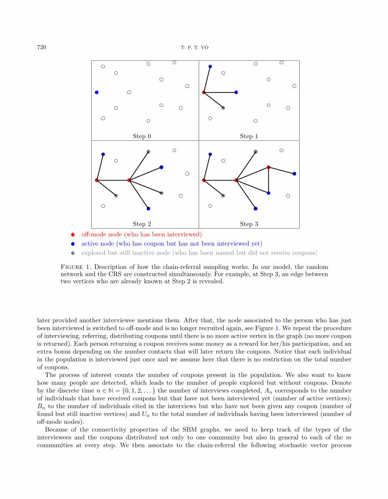
The CRS relies on a random peer-recruitment process. To handle the two sources of randomness, the graphand the exploring process on it are constructed simultaneously. In the construction, the vertices of the graphwill be in 3 different states: inactive vertices that have not being contacted for interviews, active vertices thatconstitute the next interviewees and off-mode vertices that have been already interviewed. The idea to describethe random graph as a Markov exploration process with active, explored and unexplored nodes is classical inrandom graphs theory. It has been used as a convenient technique to expose the connections inside a cluster,especially to discover the giant component in a random graph models, for example see [11, 27]. In our case,there is a slight difference in the recruiting process: the number of nodes being switched to the active modeis set to be bounded by a constant. This trick helps to improve the bias towards high-degree nodes in thepopulation (see [18]). At the beginning of the survey, all individuals in the population are hidden and aremarked as inactive vertices. We choose some people as seeds of the investigation and activate them. During theinterview these individuals name their contacts and a maximum number c of coupons are distributed to thelatter, who become active nodes. One by one, every carrier of a coupon can come to a private interview and isasked in turn to give the names of her/his peers. Whenever a new person is named, one edge connecting theinterviewee and her/his contact is added but they remain inactive until they receive a coupon. After finishingthe interview, a maximum number of c new contacts receive one coupon each and are activated. So if theinterviewee names more than c people, a number of them are not given any coupon and can be still explored

720 T. P. T. VO

Figure 1. Description of how the chain-referral sampling works. In our model, the randomnetwork and the CRS are constructed simultaneously. For example, at Step 3, an edge betweentwo vertices who are already known at Step 2 is revealed.

later provided another interviewee mentions them. After that, the node associated to the person who has justbeen interviewed is switched to off-mode and is no longer recruited again, see Figure 1. We repeat the procedureof interviewing, referring, distributing coupons until there is no more active vertex in the graph (no more couponis returned). Each person returning a coupon receives some money as a reward for her/his participation, and anextra bonus depending on the number contacts that will later return the coupons. Notice that each individualin the population is interviewed just once and we assume here that there is no restriction on the total numberof coupons.

The process of interest counts the number of coupons present in the population. We also want to knowhow many people are detected, which leads to the number of people explored but without coupons. Denoteby the discrete time n ∈ N = {0, 1, 2, . . . } the number of interviews completed, An corresponds to the numberof individuals that have received coupons but that have not been interviewed yet (number of active vertices);Bn to the number of individuals cited in the interviews but who have not been given any coupon (number offound but still inactive vertices) and Un to the total number of individuals having been interviewed (number ofoff-mode nodes).

Because of the connectivity properties of the SBM graphs, we need to keep track of the types of theinterviewees and the coupons distributed not only to one community but also in general to each of the mcommunities at every step. We then associate to the chain-referral the following stochastic vector process

CHAIN-REFERRAL SAMPLING ON STOCHASTIC BLOCK MODELS 721

Xn := (An, Bn, Un), n ∈ N:

Xn :=

AnBnUn

=

A(1)n · · · A

(m)n

B(1)n · · · B

(m)n

U(1)n · · · U

(m)n

, n ∈ N,

where A(l)n (resp. B

(l)n and u

(l)n ) corresponds to the number of active nodes (resp. of found but inactive nodes

and of off-mode nodes) of type l at step n. In all the paper, we will use the notation (X1,(l)n , X

2,(l)n , X

3,(l)n ) =

(A(l)n , B

(l)n , U

(l)n ).

The main object of the paper is to establish an approximation result when the size N of the SBM graphtends to infinity. In this case, the chain-referral process correctly renormalized is:

XNt :=

1

NXbNtc =

(AbNtc

N,BbNtc

N,UbNtc

N

)∈ [0, 1]3×m, t ∈ [0, 1]. (1.1)

In all the paper, we consider spaces Rd equipped with the L1-norm defined for x = (x1, . . . , xd) as ‖x‖ =∑dk=1 |xk|. For all N , the process XN

· lives in the space of cadlag processes D([0, 1], [0, 1]3×m) equipped withSkorokhod topology (see [13, 20, 22]).

There exist to our knowledge a few works of studying CRS form a probabilistic point of view, for example,Athreya and Rollin [3]. In their work, they obtained a result in a slightly different framework: they considerrandom walks on the limiting graphon to construct a sequence of sub-graphs, which converges almost surely tothe graphon underlying the network in the cut-metric. Whereas we take here to the limit both the graph and itsexploring random walk simultaneously. The main result of this paper is that the process (XN

. )N converges toa system of ordinary differential equations (ODEs). There has also been literature on random walks exploringgraphs possibly with different mechanism (see [7, 12] for instance). Here we allow the exploring Markov processto branch. Also, our process bares similarities with epidemics spreading on graphs (see [6, 9, 21, 26]) but withthe additional constraint of a maximum number of distributed coupons here.

The CRS is constructed by the similar principle of an epidemic spread and starts with a single individual.There are two main phases of evolution (see [6]): the initial phase is well approximated by a branching process(which we are neglecting here) and the second phase is when the stochastic process is approximated by andeterministic curve. In this paper, we focus on the second phase, but let us comment quickly on the first phase.In the sequel, we will assume that:

Assumption 1.2. For each `, k ∈ {1, . . . ,m}, denote µ`k = λ`kπk. We assume that the matrix µ =(µ`k)`,k∈{1,...,m} is irreducible and the largest eigenvalue of µ is larger than 1.

Remark 1.3. Under the Assumption 1.2, from the proof of Theorem 3.2 of Barbour and Reinert [6], the earlystages of the CRS is now can be associated approximated by a multitype branching process with the offspringdistributions determined by the matrix µ. Thanks to the Assumption 1.2 the multitype branching processassociated with the offspring matrix µ is supercritical. The analogous results for the extinction probability andfor the number of offspring at the nth generation as in the single branching process have been proved in Chapter5 of [2]: the mean matrix of the population size at time n is proportional to µn. And follow the claim (3.11) ofBarbour and Reinert [6], we can deduce that if we start with a single individual, then after a finite steps, wecan reach a positive fraction of explored individuals in the population with a positive probability.

Assumption 1.4. Set a0, b0, u0 ∈ [0, 1]m, a0 = (a(1)0 , . . . , a

(m)0 ) such that

∑mi=1 a

(i)0 = ‖a0‖ ∈ [0, 1], and set

b0, u0 ∈ [0, 1]m, with b0 = (0, . . . , 0) and u0 = (0, . . . , 0). We assume that the sequence XN0 = 1

NX0 converges inprobability to the vector (a0, b0, u0), as N → +∞.

722 T. P. T. VO

It means that the initial number of individuals with type i at the beginning of the survey is approx-

imately ba(i)0 Nc. A possible way to initializing the process is to draw A0 from a multinomial distribution

M(b‖a0‖Nc;π1, . . . , πm).

Theorem 1.5. Under the Assumptions 1.2 and 1.4, we have: when N tends to infinity, the process

(XN· )N converges in distribution in D([0, 1], [0, 1]3×m) to a deterministic vectorial function x = (x

(l)· )1≤l≤m =

(a(l)· , b

(l)· , u

(l)· )1≤l≤m in C([0, 1], [0, 1]3×m), which is the unique solution of the system of differential equations

xt = x0 +

∫ t

0

f(xs)ds, (1.2)

where f(xs) := (fil(xs)) 1≤i≤31≤l≤m

has an explicit formula described as follows. Denote

t0 := inf{t ∈ [0, 1] : ‖at‖ := a(1)t + . . .+ a

(m)t = 0}. (1.3)

For s ∈ [0, t0],

f1l(xs) =

m∑k=1

a(k)s

‖as‖λk,lsΛks

(c−

c∑h=0

(c− h)(Λks)h

h!e−Λk

s

)− a

(l)s

‖as‖; (1.4)

f2l(xs) =

m∑k=1

a(k)s

‖as‖µk,ls −

m∑k=1

a(k)s

‖as‖λk,lsΛks

(c−

c∑h=0

(c− h)(Λks)h

h!e−Λk

s

); (1.5)

f3l(xs) =a

(l)s

‖as‖; (1.6)

with

λk,ls := λkl

(πl − a(l)

s − u(l)s

); Λks :=

m∑l=1

λk,ls and µk,ls := λkl(πl − a(l)s − b(l)s − u(l)

s ). (1.7)

For s ∈ [t0, 1], f(xs) = f(xt0).

Remark 1.6. Notice that in this model, the time corresponds to the fraction of the population interviewed.The time t0 is the first time at which |at| reaches 0 and can be seen as the proportion of the populationinterviewed when there is no more coupon to keep the CRS going. Necessarily, t0 ≤ 1. We see that ‖at‖ = 0

only if a(1)t = . . . = a

(m)t = 0. It implies that f(xt) = 0,∀t ∈ [t0, 1]. Then, the solution of the system of ODEs

(1.5) becomes constant over the interval [t0, 1].

The rest of this paper is organized in the following manner. First, in Section 2, we give a precise description ofthe chain-referral process on a SBM random graph. This relies heavily on the structure of the random graph thatwe construct progressively when the exploration process spreads on it. In Section 3, we prove the limit theorem.The proof uses limit theory of cadlag semi-martingale vector processes equipped with Skorokhod topology (see[13]) and Poisson approximations (see [5]). Then in Section 4, we present simulation results of the stochasticprocess and the solution of the system of limiting ODEs. We conclude with some discussions on the impacts ofchanging parameters of the models on the evolution of the chain-referral process.

CHAIN-REFERRAL SAMPLING ON STOCHASTIC BLOCK MODELS 723

2. Definition of the chain-referral process

Let us describe the dynamics of X = (Xn)n∈N. Recall that ‖An‖ :=∑ml=1A

(l)n is the total number of

individuals having coupons but who have not yet been interviewed. We start with A0 seeds, whose typesare chosen independently according to π. A0 is an m-dimensional random vector with multinomial dis-

tribution M(b‖a0‖Nc;π1, . . . , πm), i.e. P((A

(1)0 , . . . , A

(m)0 ) = (k1, . . . , km)

)= πk11 . . . πkmm , ki ∈ N such that∑m

i=1 ki = b‖a0‖Nc and Assumption 1.4 is satisfied. Also B0 = U0 = (0, . . . , 0) and we set X0 = (A0, B0, U0).We now define Xn given the state Xn−1 previous to the nth-interview and given the number N1, . . . , Nm

of nodes of each type. At step n ≥ 1, after the nth-interview, the type of the upcoming interviewee is chosenuniformly at random according to the number of active coupons of each type in the present time. To choose the

type of the next interviewee, we define an m-dimensional vector In := (I(1)n , . . . , I

(m)n ), which takes value 1 at

coordinate l and 0 elsewhere if the nth interviewee belongs to block l. This nth-interviewee is chosen uniformlyamong the ‖An−1‖ active coupons of m types i.e. In has multinomial distribution

In = (I(1)n , . . . , I(m)

n )(d)= M

(1;

A(1)n−1

‖An−1‖, . . . ,

A(m)n−1

‖An−1‖

). (2.1)

If the chosen one belongs to block [l], A(l)n is reduced by 1 and a number of new coupons distributed are added

up, depending on how many new contacts he/she has. In the meantime, the number of interviewees of type

l is increased by 1. i.e. U(l)n = U

(l)n−1 + I

(l)n . Among the new contacts of the nth−interviewee, define H

(l)n the

number of new contacts of type l, who have not been mentioned before; K(l)n the number of new contacts of

type l whose identities are already known but who are still inactive. The H(l)n new connections are chosen

independently among Nl −A(l)n−1 −B

(l)n−1 − U

(l)n individuals in the hidden population where probability of each

successful connection is∑mk=1 I

(k)n pkl. Hence, conditioning on (N1, . . . , Nm), Xn−1, the random variable H

(l)n

follows the binomial distribution:

H(l)n

(d)= Bin

(Nl −A(l)

n−1 −B(l)n−1 − U (l)

n ,

m∑k=1

I(k)n pkl

). (2.2)

And the K(l)n individuals are chosen independently of H

(l)n from B

(l)n−1 individuals and independently of the others

with probability∑mk=1 I

(k)n pkl. In that way, conditioning on (N1, . . . , Nm), Xn−1, K

(l)n also has the binomial

distribution:

K(l)n

(d)= Bin

(B

(l)n−1,

m∑k=1

I(k)n pkl

). (2.3)

In total, there are Zn := Hn + Kn candidates, who can possibly receive coupons at step n. Notice that,

conditioning on (N1, . . . , Nm), Xn−1, (H(l)n )l=1,...,m and (K

(l)n )l=1,...,m are independent, henceforth,

Z(l)n

(d)= Bin

(Nl −A(l)

n−1 − U (l)n ,

m∑k=1

I(k)n pkl

). (2.4)

Let Cn = (C(1)n , . . . , C

(m)n ) (l = 1, . . . ,m) be the numbers of coupons that are distributed at step n. By the

setting of the survey, the total coupons |Cn| must be maximum c. If the number Zn of candidates is less than orequal to c, we deliver exactly Zn coupons. Otherwise, we choose new people to be enrolled in the study by an

m−dimensional random variable C′(l)n = (C

′(1)n , . . . , C

′(m)n ) having the multivariate hypergeometric distribution

724 T. P. T. VO

with parameters (m; c, (Z(1)n , . . . , Z

(m)n )) and the support {(c1, . . . , cm) ∈ Nm : ∀l ≤ m, cl ≤ Z(l)

n ,m∑l=1

ci = c}, that

is

P(

(C ′(1)n , . . . , C ′(m)

n ) = (c1, . . . , cm))

=

m∏l=1

(Z(l)

ncl

)(∑m

l=1 Z(l)n

c

) .In another words,

C(l)n :=

{Z

(l)n if

∑ml=1 Z

(l)n ≤ c

C′(l)n otherwise

. (2.5)

Let define by

n0 := inf{n ∈ {1, . . . , N}, An = 0} (2.6)

the first step that |An| reaches zero. The dynamics of Xn can be described by the following recursion:An = An−1 − In + Cn

Bn = Bn−1 +Hn − CnUn =

n∑i=1

Ii

, for n ∈ {1, . . . , n0} (2.7)

and Xn = Xn−1 when n > n0.

The random network is progressively discovered when the referrals chain process explores it.

Proposition 2.1. Consider the discrete-time process (Xn)1≤n≤N defined in (2.7). For n ∈ N, we denote byFn := σ

({Xi, i ≤ n, (N1, . . . , Nm)}

)the canonical filtration associated with (Xn)1≤n≤N . Then the process (Xn)n

is an inhomogeneous Markov chain with respect to the filtration (Fn)n.

Proof. The proposition is deduced from the recursion (2.7) of (Xn)1≤n≤N and the fact that the random variablesCn, In, Hn are defined conditionally on Xn−1 and (N1, . . . , Nm). The fact that the Markov process is inhomo-geneous comes from the setting of the CRS survey: there is no replacement in the recruitment procedure. For

example, when m = 1, the definition of H(l)n in (2.2) depends on time as U

(l)n = n.

3. Asymptotic behavior of the chain-referral process

Let us now consider the renormalized chain-referral process given in (1.1) in the time interval [0, t0]. Themain theorem (Thm. 1.5) shows the convergence of the sequence (XN

· )N to a deterministic process. For this, welook for an expression of the equations (2.7) as a vector of semi-martingales. We start by writing the Markovchain (Xn)1≤n≤N as the sum of its increments in discrete time.

Xn = X0 +

n∑i=1

(Xi −Xi−1) =

A0

B0

U0

+

n∑i=1

Ci − IiHi − Ci

Ii

.

Each element of the increment Xn+1 − Xn are binomial variables conditioned on all the events having beenoccurring until step n. When we fix n and let N tend to infinity, the conditional binomial random variables can

CHAIN-REFERRAL SAMPLING ON STOCHASTIC BLOCK MODELS 725

be approximated by some Poisson random variables. The normalization XNt of Xn becomes:

XNt =

1

N

A0

B0

U0

+1

N

bNtc∑i=1

Ci − IiHi − Ci

Ii

.

The Doob decomposition of the renormalized processes (XNt )t∈[0,t0] given in Section 3.1 consists of a finite

variation process and an L2-martingale. We use Aldous criteria (conditionally on the past see e.g. [13, 24]) toshow the tightness of the distributions of these processes in Section 3.2. Once the tightness is established, weidentify the limiting values of this tight sequence and finally we prove that the limiting values of all convergingsubsequences are the same, hence it is the limit of processes (XN

· )N . This proves Theorem 1.5.Denote by (FNt )t∈[0,1] := (FbNtc)t∈[0,1] the canonical filtration associated to (XN

t )t∈[0,1].

3.1. Doob’s decomposition

Lemma 3.1. The process (XNt )t∈[0,1] admits the Doob’s decomposition: XN

t = XN0 + ∆N

t +MNt , XN

0 = 1NX0.

(∆Nt )t∈[0,1] is an FNt −predictable process defined by

∆Nt =

∆N,1t

∆N,2t

∆N,3t

=1

N

bNtc∑n=1

E[Cn − In|Fn−1]E[Hn − Cn|Fn−1]

E[In|Fn−1]

; (3.1)

(MNt )t∈[0,1] is an FNt − square integrable centered martingale with quadratic variation process (〈MN

· 〉t)t∈[0,1]

given by: for every (l, k) ∈ {1, . . . ,m}2,

〈M (l),N· ,M

(k),N· 〉t =

1

N2

bNtc∑n=1

E

[(X(l)n − E[X(l)

n |Fn−1])(

X(k)n − E[X(k)

n |Fn−1])T ∣∣∣∣Fn−1

], t ∈ [0, 1] (3.2)

where X is a column vector and XT is its transpose.

Proof. In order to obtain the Doob’s decomposition, we write for t ∈ [0, 1],

XNt =

X0

N+

1

N

bNtc∑n=1

(Xn −Xn−1)

= XN0 +

1

N

bNtc∑n=1

E[Xn −Xn−1|Fn−1] +1

N

bNtc∑n=1

(Xn −Xn−1 − E[Xn −Xn−1|Fn−1])

= XN0 + ∆N

t +MNt .

It is clear that the conditional expectations above are all well-defined since the components of Xn and Xn−1

are all bounded by N , that ∆Nt is FNt −predictable and that (MN

t )t∈[0,1] is an FNt −martingale. We first checkthat (∆N

· )N is a sequence of finite variation processes and then we can conclude that XNt = XN

0 + ∆Nt +MN

t

is the Doob’s decomposition.Denote by λ := max

l,k∈{1,...,m}λkl. Notice that

‖E[An −An−1|Fn−1‖ = ‖E[Cn − In|Fn−1‖ ≤ c, (3.3)

‖E[Bn −Bn−1|Fn−1‖ = ‖E[Hn − Cn|Fn−1‖ ≤ m( maxl,k∈{1,...,m}

λkl) + c = mλ+ c, (3.4)

‖E[Un − Un−1|Fn−1‖ ≤ 1, (3.5)

726 T. P. T. VO

then ‖E[Xn −Xn−1|Fn−1]‖ ≤ 2c+mλ+ 1. So the total variation of (∆Nt )t∈[0,1] is

V N (∆Nt ) =

1

N

bNtc∑n=1

‖∆Nnt/N −∆N

(n−1)t/N‖ =1

N

bNtc∑n=1

‖E[Xn −Xn−1|Fn−1]‖ ≤ (2c+mλ+ 1)t,

which is finite. It follows that (∆Nt )t∈[0,1] is an FNt − predictable with finite variations.

The quadratic variation of (MNt )t∈[0,1] is computed as follow. For every k, l = 1, . . . ,m

M(l),Nt

(M

(k),Nt

)T=

1

N2

bNtc∑n=1

(X(l)n −X

(l)n−1 − E[X(l)

n −X(l)n−1|Fn−1]

)(X(k)n −X(k)

n−1 − E[X(k)n −X(k)

n−1|Fn−1])T

+1

N2

bNtc∑n=1

bNtc∑n′=1n′ 6=n

(X(l)n −X

(l)n−1 − E[X(l)

n −X(l)n−1|Fn−1]

)(X

(k)n′ −X

(k)n′−1 − E[X

(k)n′ −X

(k)n′−1|Fn′−1]

)T=: LNt + L′Nt .

The term L′Nt is an FNt −martingale since whenever n′ < n,(X

(k)n′ −X

(k)n′−1 − E[X

(k)n′ −X

(k)n′−1|Fn′−1]

)is

Fn−1−measurable. To see that the quadratic variation of MNt has the form (3.2), we write the term LNt

as follows:

LNt :=1

N2

bNtc∑n=1

E

[(X(l)n − E[X(l)

n |Fn−1])(

X(k)n − E[X(k)

n |Fn−1])T ∣∣∣∣Fn−1

]

+1

N2

bNtc∑n=1

(X(l)n − E[X(l)

n |Fn−1])(

X(k)n − E[X(k)

n |Fn−1])T

− 1

N2

bNtc∑n=1

E

[(X(l)n − E[X(l)

n |Fn−1])(

X(k)n − E[X(k)

n |Fn−1])T ∣∣∣∣Fn−1

]

=1

N2

bNtc∑n=1

E

[(X(l)n − E[X(l)

n |Fn−1])(

X(k)n − E[X(k)

n |Fn−1])T ∣∣∣∣Fn−1

]+ L′′Nt = 〈MN 〉t + L′′Nt .

As a result,

M(l),Nt

(M

(k),Nt

)T= 〈MN 〉t + L′Nt + L′′Nt . (3.6)

Because both L′Nt and L′′Nt are FNt −martingale, L′Nt + L′′Nt is an FNt −martingale as well. The term (〈MN 〉t)tis FNt −adapted with the variation

V N (〈MN· 〉t) =

1

N2

bNtc∑n=1

m∑k,l=1

∥∥∥∥E

[(X(l)n − E[X(l)

n |Fn−1])(

X(k)n − E[X(k)

n |Fn−1])T ∣∣∣∣Fn−1

]∥∥∥∥ . (3.7)

The integrand in the right hand side is the conditional covariance between X(l)n and X

(k)n conditionally to Fn−1.

Because X(l)n and X

(k)n are vectors, this covariance is a matrix of size 3× 3 and for 1 ≤ i, j ≤ 3, the term (i, j)

CHAIN-REFERRAL SAMPLING ON STOCHASTIC BLOCK MODELS 727

of this matrix is:

E

[(Xi,(l)n − E[Xi,(l)

n |Fn−1])(

Xj,(k)n − E[Xj,(k)

n |Fn−1]) ∣∣∣∣Fn−1

]≤(

Var(Xi,(l)n −Xi,(l)

n−1|Fn−1))1/2 (

Var(Xj,(k)n −Xj,(k)

n−1 |Fn−1))1/2

,

by the Cauchy-Schwarz inequality. Thus:

V N (〈MN· 〉t) ≤

1

N2

bNtc∑n=1

m∑k,l=1

∣∣∣∣∣∣3∑

i,j=1

(Var(Xi,(l)

n −Xi,(l)n−1|Fn−1)

)1/2 (Var(Xj,(k)

n −Xj,(k)n−1 |Fn−1)

)1/2

∣∣∣∣∣∣ ,where (X

1,(l)n , X

2,(l)n , X

3,(l)n ) = (A

(l)n , B

(l)n , U

(l)n ). By Cauchy-Schwarz’s inequality, we have

3∑i,j=1

(Var(Xi,(l)

n −Xi,(l)n−1|Fn−1)

)1/2 (Var(Xj,(k)

n −Xj,(k)n−1 |Fn−1)

)1/2

=

(3∑i=1

(Var(Xi,(l)

n −Xi,(l)n−1|Fn−1)

)1/2) 3∑

j=1

(Var(Xj,(k)

n −Xj,(k)n−1 |Fn−1)

)1/2

≤ 3

2

3∑i=1

(Var(Xi,(l)

n −Xi,(l)n−1|Fn−1) + Var(Xi,(k)

n −Xi,(k)n−1 |Fn−1)

). (3.8)

From (3.3)–(3.5) and by Cauchy-Schwarz’s inequality, we obtain the following inequalities

Var(C(l)n − I(l)

n |Fn−1) ≤ c2, Var(H(l)n − C(l)

n |Fn−1) ≤ 2( maxl,k∈{1,...,m}

λ2lk + c2), Var(I(l)

n |Fn−1) ≤ 1. (3.9)

As a consequence,

V N(〈MN· 〉t

)≤ 1

N2

bNtc∑n=1

3m2(c2 + 2( maxl,k∈{1,...,m}

λ2lk + c2) + 1) ≤ 1

N3m2(3c2 + 2λ2 + 1) <∞.

Thus, the proof of the lemma is completed.

3.2. Tightness of the renormalized process

Lemma 3.2. The sequence of processes (XN· )N is tight in the Skorokhod space D([0, 1], [0, 1]3×m).

Proof. To prove the tightness of (XN· )N , we use the criteria of tightness for semi-martingales in ([24], Thm.

2.3.2 (Rebolledo)): first, we verify the marginal tightness of each sequence (XNt )N for each t ∈ [0, 1], then we

show the tightness for each process in the Doob’s decomposition of XN , the finite variation process (∆N )Nand the quadratic variation of the martingale (MN )N . For any t ∈ [0, 1], the tightness of marginal sequence(XN

t )N is easily deduced from the compactness of a sequence of random variables taking values in a compact set[0, 1]3×m. Since the sequence of martigales (MN )N is proved to be convergent (to zero) in L2 as N →∞ (whichis done by Prop. 3.3), we have the tightness of (MN )N . Thus, it is sufficient to check the tightness conditionfor the modulus of continuity of (∆N )N (see, e.g., [8], Thm. 13.2, p. 139).

728 T. P. T. VO

For all 0 < δ < 1 and for every s, t ∈ [0, 1] such that |t− s| < δ, we have that

‖∆Nt −∆N

s ‖ =

∥∥∥∥∥∥ 1

N

bNtc∑n=bNsc+1

E[Xn −Xn−1|Fn−1]

∥∥∥∥∥∥ ≤ 1

N

bNtc∑n=bNsc+1

‖E[Xn −Xn−1|Fn−1]‖.

By (3.3)–(3.5), we get

‖∆Nt −∆N

s ‖ ≤bNtc − bNsc

N(c+mλ+ c+ 1) ≤ (2c+mλ+ 1)

(δ +

1

N

).

Thus, for each ε > 0, choose δ0 ≤ ε2(2c+mλ+1) , we have that

P

sup|t−s|<δ

0≤s<t≤1

‖∆Nt −∆N

s ‖ > ε

= 0, ∀δ ≤ δ0,∀N >1

δ0,

which allows us to conclude that the sequence (∆N· )N is tight and finishes the proof of the lemma.

To complete the proof of Lemma 3.2, we now prove that:

Proposition 3.3. The sequence of martingale (MNt , t ∈ [0, 1])N converges locally uniformly in t to 0 in L2, as

N goes to infinity.

Proof. Consider the quadratic variation of (MN· )N : According to the formula (3.2), we apply the Cauchy–

Schwarz’s inequality and then use the inequality (3.8) to obtain that for every t ∈ [0, 1],

‖〈M (l),N ,M (k),N 〉t‖ =

∥∥∥∥∥∥ 1

N2

bNtc∑n=1

E

[(X(l)n − E[X(l)

n |Fn−1])(

X(k)n − E[X(k)

n |Fn−1])T ∣∣∣∣Fn−1

]∥∥∥∥∥∥≤ 1

N2

bNtc∑n=1

∣∣∣∣∣∣3∑

i,j=1

(Var(Xi,(l)

n −Xi,(l)n−1|Fn−1)

)1/2 (Var(Xj,(k)

n −Xj,(k)n−1 |Fn−1)

)1/2

∣∣∣∣∣∣≤ 1

N2

bNtc∑n=1

3

2

3∑i=1

(Var(Xi,(l)

n −Xi,(l)n−1|Fn−1) + Var(Xi,(k)

n −Xi,(k)n−1 |Fn−1)

),

where (X1,(l)n , X

2,(l)n , X

3,(l)n ) = (A

(l)n , B

(l)n , U

(l)n ). From (3.3)–(3.5) and (3.9), we deduce that

‖〈MN· 〉t‖ ≤

1

N2

bNtc∑n=1

3m2

2

(c2 + 2( max

l,k∈{1,...,m}λ2lk + c2) + 1

)≤ 1

N

3m2

2(3c2 + 2λ2 + 1)t. (3.10)

Applying the Doob’s inequality for martingale, for every t ∈ [0, 1], we have

E

[max

0≤s≤t‖MN

s ‖2]≤ 4E

[‖〈MN

· 〉t‖]≤ 1

N6m2(3c2 + 2λ2 + 1)→ 0 as N →∞.

This concludes the proof of Proposition 3.3 and hence of Lemma 3.2.

CHAIN-REFERRAL SAMPLING ON STOCHASTIC BLOCK MODELS 729

3.3. Identify the limiting value

Since the sequence (XN· )N is tight, for any limiting value x = (a, b, u) of the sequence (XN )N , there exists an

increasing sequence (ϕN )N in N such that (XϕN· )N converges in distribution to x in D([0, 1], [0, 1]3×m). Because

the sizes of the jumps converge to zero with N , the limit is in fact in C([0, 1], [0, 1]3×m). We want to identify thatlimit. In order to simplify the notations, we also write the subsequence (XϕN

· )N as (XN· )N = (AN· , B

N· , U

N· )N .

We consider separately the martingale and finite variation parts. Proposition 3.3 implies that the sequencemartingale (MN

· )N converges to 0 in distribution and hence (MN )N converges to zero in probability. It remainsto find the limit of the finite variation process (∆N

· )N given in equation (3.1) and prove that the limit foundis the same (which is done later in the proof for the uniqueness of the system of the ODEs (1.5)) for everyconvergent subsequence extracted from the tight sequence (XN )N .

Proposition 3.4. When N goes to infinity, we have the following convergences in distribution inD([0, 1], [0, 1]3×m):

1

N

bNtc∑n=1

E[C(l)n |Fn−1]

(d)→∫ t

0

{m∑k=1

a(k)s

‖as‖λk,lsΛks

(c−

c∑h=0

(c− h)(Λks)h

h!e−Λk

s

)}ds, (3.11)

1

N

bNtc∑n=1

E[H(l)n |Fn−1]

(d)−→∫ t

0

m∑k=1

a(k)s

‖as‖µk,ls ds, (3.12)

1

N

bNtc∑n=1

E[I(l)n |Fn−1] =

1

N

bNtc∑n=1

(A

(l)n−1

N

)/(‖An−1‖N

)(d)−→

t∫0

a(l)s

‖as‖ds, (3.13)

where λk,ls ,Λks , µk,ls are defined as in Theorem 1.5. This provides the convergence of (∆N

· )N to a solution x. of(1.2).

Since the limits are deterministic, the convergences hold in probability. Moreover the uniqueness of thesolution of (1.2) will be proved later, which will imply the convergence of the whole sequence (XN

· )N to thissolution.

Proof. Recall that since the sequence (XN. )N is tight, we have extracted a converging subsequence also denoted

by (XN. )N of which we study the limit.

The proof of the Proposition 3.4 is separated into three steps.Step 1: We consider the most complicated term E[Cn|Fn−1]. We prove that: for each l ∈ {0, . . . ,m},

∣∣∣∣∣E[C(l)n |Fn−1]− λ

(l)n

Λn

(c−

c∑h=0

(c− h)(Λn)h

h!e−Λn

)∣∣∣∣∣ ≤ m(c+ 1)λ

N, (3.14)

where

λ(l)n :=

(m∑k=1

I(k)n λkl

)(NlN−A

(l)n−1

N− U

(l)n

N

)and Λn :=

m∑j=1

λ(j)n . (3.15)

Notice that Λn = 0 only if for each l ∈ {1, . . . ,m}, λ(l)n = 0. It happens when A

(l)n−1 + U

(l)n = Nl, meaning

that all the nodes of type l have been discovered. In this case, C(l)n = 0 and (3.14) is satisfied.

730 T. P. T. VO

Let us write

E[C(l)n |Fn−1] = E

[Z(l)n 1∑m

j=1 Z(j)n ≤c

∣∣Fn−1

]+ E

[cZ

(l)n∑m

j=1 Z(j)n

1∑mj=1 Z

(j)n >c

∣∣∣∣Fn−1

]. (3.16)

For every l = 1, . . . ,m and every fixed n, when all the parameters are positive, we have that (Nl − A(l)n−1 −

U(l)n )

N→∞−→a.s.

+∞. Then we work conditionally on Nl, A(l)n−1, U

(l)n and I

(l)n and use the Poisson approximation (e.g.

see Eq. (1.23) and Thm. 2.A, 2.B by Barbour, Holst and Janson in [5]) for the approximation: the binomial

random variable Z(l)n may be approximated by a Poisson random variable Z

(l)n

(d)= P

((∑mk=1 I

(k)n λkl)(

Nl

N −A

(l)n−1

N −U(l)

n

N ))

such that

dTV(Z(l)n , Z(l)

n ) ≤ 2

(Nl −A(l)n − U (l)

n )

(∑mk=1 I

(k)n λkl

N

) Nl−A(l)n −U

(l)n∑

i=1

(∑mk=1 I

(k)n λkl

N

)2

≤2 max

k,lλkl

N=

2λ

N.

As a consequence, the first term in the right hand side of (3.16) can be approximated as∣∣∣∣E [Z(l)n 1∑m

j=1 Z(j)n ≤c

∣∣∣∣Fn−1

]− E

[Z(l)n 1∑m

j=1 Z(j)n ≤c

∣∣∣∣Fn−1

]∣∣∣∣ ≤ 2mcλ

N, (3.17)

and ∣∣∣∣∣E[

Z(l)n∑m

j=1 Z(j)n

1∑mj=1 Z

(j)n >c

∣∣∣∣Fn−1

]− E

[Z

(l)n∑m

j=1 Z(j)n

1∑mj=1 Z

(j)n >c

∣∣∣∣Fn−1

]∣∣∣∣∣ ≤ 2mλ

N. (3.18)

It follows that we need to deal with the Poisson random variables Z(l)n (l ∈ {1, . . . ,m}). Because of the result

that the sum of two independent Poisson random variables is a Poisson random variable whose parameter is

the sum of the two parameters, we have that∑j 6=l Z

(j)n =: Z

(l)n has a Poisson distribution with parameter

λ(l)n :=

∑j 6=l λ

(j)n . And hence,

E

[Z(l)n 1∑m

j=1 Z(j)n ≤c

∣∣Fn−1

]=

c∑h=1

h∑h1=1

h1(λ

(l)n )h1(λ

(l)n )h−h1

h1!(h− h1)!e−Λn

= λ(l)n

c∑h=1

(Λn)h−1

(h− 1)!e−Λn = λ(l)

n

c∑h=0

h

Λn

(Λn)h

h!e−Λn

and

E

[Z

(l)n∑m

j=1 Z(j)n

1∑mj=1 Z

(j)n >c

∣∣∣∣Fn−1

]=

∞∑h=c+1

h∑k=0

k

h

(λ(l)n )k

k!

(λ(l)n )h−k

(h− k)!e−λ

(l)n e−λ

(l)n

= λ(l)n

∞∑h=c+1

h−1∑k=0

1

h

(λ(l)n )k

k!

(λ(l)n )h−1−k

(h− 1− k)!e−λ

(l)n e−λ

(l)n

CHAIN-REFERRAL SAMPLING ON STOCHASTIC BLOCK MODELS 731

= λ(l)n

∞∑h=c+1

1

h

(λ(l)n + λ

(l)n )h−1

(h− 1)!e−(λ(l)

n +λ(l)n ) =

λ(l)n

Λn

∞∑h=c+1

(Λn)h

h!e−Λn

=λ

(l)n

Λn(1−

c∑h=0

(Λn)h

h!e−Λn). (3.19)

Using (3.16), we obtain:

E[C(l)n |Fn−1] = E

[Z(l)n 1∑m

j=1 Z(j)n ≤c

+Z

(l)n∑m

j=1 Z(j)n

1∑mj=1 Z

(j)n >c

∣∣∣∣Fn−1

]=λ

(l)n

Λn

(c−

c∑h=0

(c− h)(Λn)h

h!e−Λn

),

which finishes Step 1.Step 2: We decompose the second term in the left hand side of (3.14) as follows:

λ(l)n

Λn

(c−

c∑h=0

(c− h)(Λn)h

h!e−Λn

)= α(l)

n + ξ(l)n , l = 1, . . . ,m. (3.20)

with

α(l)n := E

[λ

(l)n

Λn

(c−

c∑h=0

(c− h)(Λn)h

h!e−Λn

)∣∣∣∣Fn−1

]

ξ(l)n :=

λ(l)n

Λn

(c−

c∑h=0

(c− h)(Λn)h

h!e−Λn

)− E

[λ

(l)n

Λn

(c−

c∑h=0

(c− h)(Λn)h

h!e−Λn

)∣∣∣∣Fn−1

].

By writing

α(l)n =

m∑k=1

P(I(k)n = 1)

λk,lnΛkn

(c−

c∑h=0

(c− h)(Λkn)h

h!e−Λk

n

),

where

λk,ln := λkl

(NlN−A

(l)n−1

N−U

(l)n−1

N−

1{k=l}

N

)and Λkn :=

m∑j=1

λk,jn (l = 1, . . . ,m), (3.21)

we obtain that for every t ∈ [0, 1],

1

N

bNtc∑n=1

α(l)n =

1

N

bNtc∑n=1

{m∑k=1

A(k)n−1

|An−1|λk,lnΛkn

(c−

c∑h=0

(c− h)(Λkn)h

h!e−Λk

n

)}. (3.22)

It is obvious that 1N

∑bNtcn=1 ξn is an FNt −martigale with the quadratic variation,

〈 1

N

bN ·c∑n=1

ξn〉t =1

N2

bNtc∑n=1

E[ξ2n|Fn−1

]≤ 1

N2

bNtc∑n=1

m(c+ 1)2 ≤ m(c+ 1)2

N.

732 T. P. T. VO

By the Doob’s inequality, we have

E

max0≤s≤t

‖ 1

N

bNtc∑n=1

ξn‖2 ≤ 4E

‖〈 1

N

bN ·c∑n=1

ξn〉t‖

≤ 4m(c+ 1)2

N

N→∞−→ 0,

which deduces that as N tends to infinity, we have that

1

N

bNtc∑n=1

ξn(L2)→ 0 (3.23)

uniformly in t ∈ [0, 1]. Together with the points given in (3.14), (3.20) and (3.23), take the limit as N →∞ inthe right hand side of (3.22), we obtain the right hand side of (3.11).Step 3: We use similar arguments as in Step 2 to obtain the limit in right hand side of (3.12). Denote by

µ(l)n :=

(m∑k=1

I(k)n λkl

)(NlN−A

(l)n−1

N−B

(l)n−1

N− U

(l)n

N

).

Recall from (2.2) that conditioning on Fn−1, H(l)n

(d)= Bin

(Nl −A(l)

n−1 −B(l)n−1 − U

(l)n ,

∑mk=1 I

(k)n λkl

N

), then

1

N

bNtc∑n=1

E[H(l)n |Fn−1] =

1

N

bNtc∑n=1

µ(l)n . (3.24)

We write

1

N

bNtc∑n=1

µ(l)n =

1

N

bNtc∑n=1

(β(l)n + ζ(l)

n ) (3.25)

with

β(l)n := E

[(m∑k=1

I(k)n λkl

)(NlN−A

(l)n−1

N−B

(l)n−1

N− U

(l)n

N

)∣∣∣∣Fn−1

];

ζ(l)n :=

(m∑k=1

I(k)n λkl

)(NlN−A

(l)n−1

N−B

(l)n−1

N− U

(l)n

N

)− E

[(m∑k=1

I(k)n λkl

)(NlN−A

(l)n−1

N−B

(l)n−1

N− U

(l)n

N

)∣∣∣∣Fn−1

].

Using a similar argument as in Step 2, we have

1

N

bNtc∑n=1

β(l)n =

1

N

bNtc∑n=1

m∑k=1

P(I(k)n = 1)λkl

(NlN−A

(l)n−1

N−B

(l)n−1

N−U

(l)n−1

N−

1{k 6=l}N

)

=1

N

bNtc∑n=1

m∑k=1

A(k)n−1

‖An−1‖µk,ln −

1

N

bNtc∑n=1

m∑k=1

AN,kn−1

‖ANn−1‖λkl

1{k 6=l}N

,

CHAIN-REFERRAL SAMPLING ON STOCHASTIC BLOCK MODELS 733

with µk,ln := λkl

(Nl

N −A

(l)n−1

N − B(l)n−1

N − U(l)n−1

N

). Then,

∣∣∣∣∣∣ 1

N

bNtc∑n=1

(β(l)n −

m∑k=1

A(k)n−1

‖An−1‖µk,ln

)∣∣∣∣∣∣ ≤ 1

N

bNtc∑n=1

m∑k=1

AN,kn−1

‖ANn−1‖λkl

1{k 6=l}N

≤ λ

N. (3.26)

Take the limit as N → +∞, we have that

limN→+∞

1

N

bNtc∑n=1

m∑k=1

A(k)n−1

‖An−1‖µk,ln =

∫ t

0

m∑k=1

a(k)s

‖as‖µk,ls ds.

Further, the FNt −martingale1

N

bN ·c∑n=1

ζ(l)n converges in L2 to 0 uniformly in t ∈ [0, 1]. Thus, (3.12) is proved.

For the proof of (3.13), by the definition of In as in (2.1), we have

1

N

bNtc∑n=1

E[I(l)n |Fn−1] =

1

N

bNtc∑n=1

A(l)n−1

‖An−1‖=

1

N

bNtc∑n=1

A(l)n−1/N

‖An−1‖/N.

Take the limit as N → +∞, we obtain the limit in the right hand side of (3.13).The preceding steps allow to conclude the proof of Proposition 3.4.

3.4. The uniqueness

It remains to prove that the limiting value x = (a, b, u) we have found is unique solution of the system of heODEs (1.2). If it is the case, then the process (XN )N admits a unique limiting value and thus converges to x.

Assume that there exist two solutions x1 and x2 to ODEs (1.2) on the interval [0, t′0], where

t′0 = inf{t ∈ [0, 1] : a1t′0

= 0 or a2t′0

= 0}.

Then using the intermediate value theorem, there exist ξij(s) ∈ [x1ij(s), x

2ij(s)] such that

‖x1t − x2

t‖ =

∥∥∥∥∫ t

0

(f(x1s)− f(x2

s))ds

∥∥∥∥ ≤ ∫ t

0

3∑i=1

m∑j=1

∣∣∣∣ ∂f∂xij (ξij(s))

∣∣∣∣ ∣∣x1ij(s)− x2

ij(s)∣∣ds

≤∫ t

0

L(s)‖x1s − x2

s‖ds,

where xks = (xij(s)) 1≤i≤31≤j≤m

(k ∈ {1, 2}) and L(s) =

3∑i=1

m∑j=1

max

∣∣∣∣ ∂f∂xij (xs)

∣∣∣∣, of which the maximum is over x(s) =

(xij(s))ij ∈ [0, 1]3m such that ∀i, j : xij ∈ [x1ij , x

2ij ], where by an abuse of notation, the bounds of interval [x1

ij , x2ij ]

can be switched depending on the minimum or maximum of the bounds.By the Gronwall’s inequality, we get

‖x1t − x2

t‖ ≤ ‖x10 − x2

0‖ exp(

∫ t

0

L(s)ds) = 0.

734 T. P. T. VO

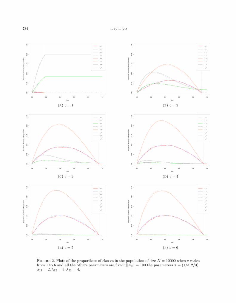
Figure 2. Plots of the proportions of classes in the population of size N = 10000 when c variesfrom 1 to 6 and all the others parameters are fixed: ‖A0‖ = 100 the parameters π = (1/3, 2/3),λ11 = 2, λ12 = 3, λ22 = 4.

CHAIN-REFERRAL SAMPLING ON STOCHASTIC BLOCK MODELS 735

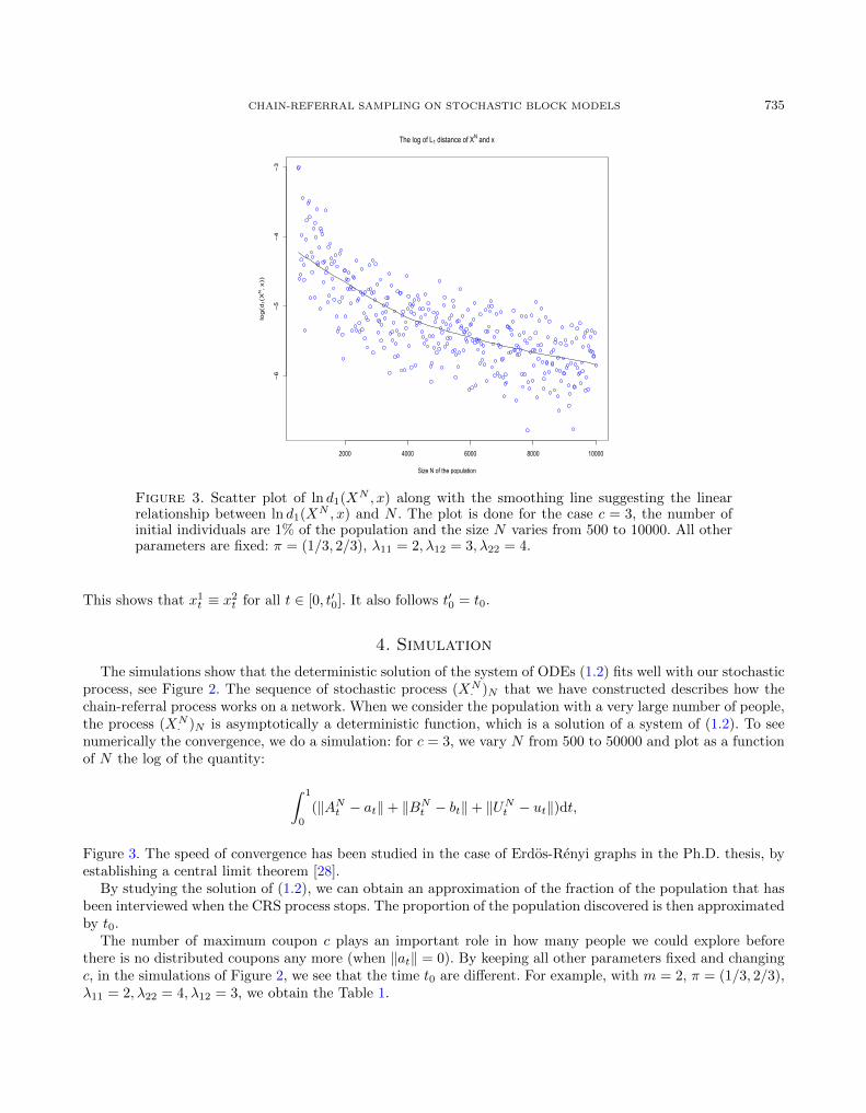
Figure 3. Scatter plot of ln d1(XN , x) along with the smoothing line suggesting the linearrelationship between ln d1(XN , x) and N . The plot is done for the case c = 3, the number ofinitial individuals are 1% of the population and the size N varies from 500 to 10000. All otherparameters are fixed: π = (1/3, 2/3), λ11 = 2, λ12 = 3, λ22 = 4.

This shows that x1t ≡ x2

t for all t ∈ [0, t′0]. It also follows t′0 = t0.

4. Simulation

The simulations show that the deterministic solution of the system of ODEs (1.2) fits well with our stochasticprocess, see Figure 2. The sequence of stochastic process (XN

· )N that we have constructed describes how thechain-referral process works on a network. When we consider the population with a very large number of people,the process (XN

· )N is asymptotically a deterministic function, which is a solution of a system of (1.2). To seenumerically the convergence, we do a simulation: for c = 3, we vary N from 500 to 50000 and plot as a functionof N the log of the quantity:

∫ 1

0

(‖ANt − at‖+ ‖BNt − bt‖+ ‖UNt − ut‖)dt,

Figure 3. The speed of convergence has been studied in the case of Erdos-Renyi graphs in the Ph.D. thesis, byestablishing a central limit theorem [28].

By studying the solution of (1.2), we can obtain an approximation of the fraction of the population that hasbeen interviewed when the CRS process stops. The proportion of the population discovered is then approximatedby t0.

The number of maximum coupon c plays an important role in how many people we could explore beforethere is no distributed coupons any more (when ‖at‖ = 0). By keeping all other parameters fixed and changingc, in the simulations of Figure 2, we see that the time t0 are different. For example, with m = 2, π = (1/3, 2/3),λ11 = 2, λ22 = 4, λ12 = 3, we obtain the Table 1.

736 T. P. T. VO

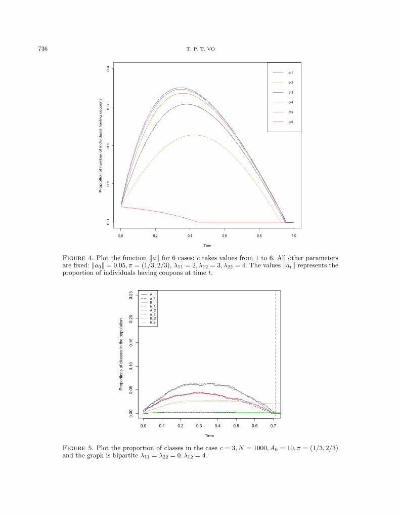
Figure 4. Plot the function ‖a‖ for 6 cases: c takes values from 1 to 6. All other parametersare fixed: ‖a0‖ = 0.05, π = (1/3, 2/3), λ11 = 2, λ12 = 3, λ22 = 4. The values ‖at‖ represents theproportion of individuals having coupons at time t.

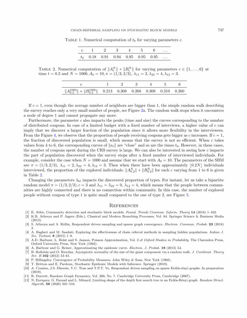
Figure 5. Plot the proportion of classes in the case c = 3, N = 1000, A0 = 10, π = (1/3, 2/3)and the graph is bipartite λ11 = λ22 = 0, λ12 = 4.

CHAIN-REFERRAL SAMPLING ON STOCHASTIC BLOCK MODELS 737

Table 1. Numerical computation of t0 for varying parameters c.

c 1 2 3 4 5 6 . . .

t0 0.18 0.91 0.94 0.95 0.95 0.95 . . .

Table 2. Numerical computation of ‖ANt ‖ + ‖BNt ‖ for varying parameters c ∈ {1, . . . , 6} attime t = 0.2 and N = 1000, A0 = 10, π = (1/3, 2/3), λ11 = 2, λ22 = 4, λ12 = 3.

c 1 2 3 4 5 6

‖A10000.2 ‖+ ‖B1000

0.2 ‖ 0.213 0.308 0.268 0.308 0.310 0.260

If c = 1, even though the average number of neighbors are bigger than 1, the simple random walk describingthe survey reaches only a very small number of people, see Figure 2a. The random walk stops when it encountersa node of degree 1 and cannot propagate any more.

Furthermore, the parameter c also impacts the peaks (time and size) the curves corresponding to the numberof distributed coupons. In case of a limited budget with a fixed number of interviews, a higher value of c canimply that we discover a larger fraction of the population since it allows more flexibility in the interviewees.From the Figure 4, we observe that the proportion of people receiving coupons gets bigger as c increases. If c = 1,the fraction of discovered population is small, which means that the survey is not so efficient. When c takesvalues from 4 to 6, the corresponding curves of ‖at‖ are “close” and so are the times t0. However, in these cases,the number of coupons spent during the CRS survey is large. We can also be interested in seeing how c impactsthe part of population discovered when the survey stops after a fixed number of interviewed individuals. Forexample, consider the case when N = 1000 and assume that we start with A0 = 10. The parameters of the SBMare π = (1/3, 2/3), λ11 = 2, λ22 = 4, λ12 = 3. Then when there have been approximately b0.2Nc individualsinterviewed, the proportion of the explored individuals: ‖AN0.2‖+ ‖BN0.2‖ for each c varying from 1 to 6 is givenin Table 2.

Changing the parameters λkl impacts the discovered proportion of types. For instant, let us take a bipartiterandom model π = (1/3, 2/3), c = 3 and λ11 = λ22 = 0, λ12 = 4, which means that the people between commu-nities are highly connected and there is no connection within community. In this case, the number of exploredpeople without coupon of type 1 is quite small compared to the one of type 2, see Figure 5.

References[1] E. Abbe, Community detection and stochastic block models. Found. Trends Commun. Inform. Theory 14 (2018) 1–162.[2] K.B. Athreya and P. Jagers (Eds.), Classical and Modern Branching Processes, Vol. 84. Springer Science & Business Media

(2012).[3] S. Athreya and A. Rollin, Respondent driven sampling and sparse graph convergence. Electron. Commun. Probab. 23 (2018)

3.[4] A. Bagheri and M. Saadati, Exploring the effectiveness of chain referral methods in sampling hidden populations. Indian J.

Sci. Technol. 8 (2015) 1–8.

[5] A.D. Barbour, L. Holst and S. Janson, Poisson Approximation, Vol. 2 of Oxford Studies in Probability. The Clarendon Press,Oxford University Press, New York (1992).

[6] A. Barbour and G. Reiner, Approximating the epidemic curve. Electron. J. Probab. 18 (2013) 54.[7] B. Bollobas and O. Riordan, Asymptotic normality of the size of the giant component via a random walk. J. Combinat. Theory

Ser. B 102 (2012) 53–61.[8] P. Billingsley, Convergence of Probability Measures. John Wiley & Sons, New York (1968).

[9] T. Britton and E. Pardoux, Stochastic Epidemic Models with Inference. Springer (2019).[10] A. Cousien, J.S. Dhersin, V.C. Tran and T.P.T. Vo, Respondent driven sampling on sparse Erdos-renyi graphs. In preparation

(2019).[11] R. Durrett, Random Graph Dynamics, Vol. 200, No. 7. Cambridge University Press, Cambridge (2007).[12] N. Enriquez, G. Faraud and L. Menard, Limiting shape of the depth first search tree in an Erdos-Renyi graph. Random Struct.

Algorith. 56 (2020) 501–516.

738 T. P. T. VO

[13] S.N. Ethier and T.G. Kurtz, Markov Processes, Characterization and Convergence. John Wiley & Sons, New York (1986).

[14] A. Gadde, E.E. Gad, S. Avestimehr and A. Ortega, Active learning for community detection in stochastic block models. In2016 IEEE International Symposium on Information Theory (ISIT) (2016) 1889–1893.

[15] M. Girvan and M.E.J. Newman, Community structure in social and biological networks. Proc. Natl. Acad. Sci. U.S.A. 99(2002) 7821–7826.

[16] L.A. Goodman, Snowball sampling. Ann. Math. Statist. (1961) 148–170.

[17] D.D. Heckathorn, Respondent-driven sampling: a new approach to the study of hidden populations. Social Probl. 44 (1997)74–99.

[18] D.D. Heckathorn, Respondent-driven sampling II: deriving valid population estimates from chain-referral samples of hiddenpopulations. Social Probl. 49 (2002) 11–34.

[19] P.W. Holland, K.B. Laskey and S. Leinhardt, Stochastic blockmodels: first steps. Social Netw. 5 (1983) 109–137.[20] A. Jakubowski, On the Skorokhod topology. Ann. Inst. Henri Poincare 22 (1986) 263–285.

[21] S. Janson, M. Luczak and P. Windridge, Law of large numbers for the SIR epidemic on a random graph with given degrees.Random Struct. Algorith. 45 (2014) 726–763.

[22] A. Joffe and M. Metivier, Weak convergence of sequences of semimartingales with applications to multitype branching processes.Adv. Appl. Probab 18 (1986) 20–65.

[23] P. Barbillon, S. Donnet, E. Lazega and A. Bar-Hen, Stochastic Block Models for Multiplex networks: an application to networksof researchers. Preprint arXiv:1501.06444 (2015).

[24] M. Metivier, Semimartingales: A Course on Stochastic Processes, Vol. 2. Walter de Gruyter (2011).

[25] A. Shaghaghi, R.S. Bhopal and A. Sheikh, Approaches to recruiting ‘hard-to-reach’ populations into research: a review of theliterature. Health Promotion Perspect. 1 (2011) 86.

[26] V.C. Tran, P. Moyal, L. Decreusefond and J.S. Dhersin, Limite en grand graphe d’un processus SIR decrivant la propagationd’une epidemie sur un reseau. Journees MAS et Journee en l’honneur de Jacques Neveu, August 2010, Talence, France (2010).

[27] R. Van Der Hofstad, Random Graphs and Complex Networks. Vol. 1. Cambridge University Press (2016).[28] T.P.T. Vo, Exploration of Random Graphs by the Respondent Driven Sampling method. Ph.D. thesis, University Paris 13

(2020).