ABSTRACTThe purpose of this study was to develop a numericalanalytical model of collinear low-speed bumper-to-bumpercrashes and use the model to perform parametric studies oflow-speed crashes and to estimate the severity of low-speedcrashes that have already occurred. The model treats the carbody as a rigid structure and the bumper as a deformablestructure attached to the vehicle. The theory used in themodel is based on Newton's Laws. The model uses an ImpactForce-Deformation (IF-D) function to determine the impactforce for a given amount of crush. The IF-D function used inthe simulation of a crash that has already occurred can betheoretical or based on the measured force-deflectioncharacteristics of the bumpers of the vehicles that wereinvolved in the actual crash. The restitution of the bumpers isaccounted for in a simulated crash through the reboundcharacteristics of the bumper system in the IF-D function.The output of the model for a numerical simulation is theacceleration vs. time information for each vehicle in thesimulated crash. Three low-speed crash tests were performedand the dynamic IF-D curve was measured in each crash. Theanalytical model was used to simulate the three low-speedcrash tests in order to demonstrate the model's ability todescribe the vehicle dynamics in a crash that has alreadyoccurred. The model is also used to perform parametricstudies that show how the structural characteristics of thevehicles' bumpers and the closing speed affect the crash pulseand to demonstrate a technique to estimate the maximumseverity of a low-speed crash that has already occurred.

INTRODUCTIONThere have been two main approaches to modeling a low-speed collinear crash between two vehicles. The firstapproach is to treat the vehicles as rigid structures and modelthe bumpers as spring/dashpot systems and then solve the

governing differential equations with the appropriate initialconditions (1, 3, 4, 7). The solution gives the accelerations ofboth vehicles during the crash. In order to simulate a specificcrash with a spring/dashpot model the appropriate stiffnessand damping coefficients must be used. The second approachhas been called the Momentum-Energy-Restitution (MER)method. This method is based on rigid body impactmechanics and uses impulse, conservation of momentum,conservation of energy and restitution to determine the ΔV ofthe vehicles in a low-speed crash (2, 5, 6). In order toestimate the ΔV for a vehicle in a specific crash the MERmethod requires a value for the coefficient of restitution (ε)and an estimate of the energy absorbed by each vehicleduring the crash. An analysis of a low-speed crash with theMER method provides a ΔV for the crash but does notprovide the acceleration vs. time information for the vehiclesduring the crash. The peak acceleration in the crash can beestimated by assuming a shape and length for the crash pulse.

Thomson and Romilly (1) treated the vehicle as a rigid massand the bumper system as a spring/dashpot system in theirsimulation model. Pendulum-to-car (VW Rabbit) crash testsand static and dynamic compression tests of the VW's piston-type energy absorbers were performed. The simulation modelwas used to calculate the VWs dynamic response in thependulum-to-car crash tests. Four different methods weredeveloped to analytically determine the linear coefficients ofthe spring/dashpot system. The damping and stiffnesscoefficients that best represented the experimental data werebased on an energy analysis of the pendulum-to-car impacts.The calculated accelerations approximated the measuredaccelerations but did not start at zero because of the constantcoefficient for the dashpot.

Bailey et al. (2) performed a series of car-to-car crash testswith vehicles whose bumpers had piston-type energyabsorbers. The MER method was used to calculate the ΔV of

Simulation Model for Low-Speed Bumper-to-Bumper Crashes

2010-01-0051Published

04/12/2010

W. R. Scott, C. Bain, S. J. Manoogian, J. M. Cormier and J. R. FunkBiodynamic Research Corporation

Copyright © 2010 SAE International

the vehicles in the crash tests. In the ΔV calculations ε wasbased on previously performed barrier impacts with the samevehicles and the energy absorbed by each vehicle wasestimated from the amount of compression of the piston-typeenergy absorber in the actual crash test. The ΔVs calculatedwith the MER method were very close to the ΔVs measuredin the crash tests.

Ojalvo and Cohen (3) reviewed vehicle-to-vehicle crash testdata of Ford Escorts that had bumpers with piston-typeenergy absorbers and concluded that a linear spring/dashpotmodel could be used to represent the dynamic response ofthese vehicles in low-speed crashes. In their model thevehicles were rigid masses and the bumpers were linearspring/dashpot systems. The simulation model was used toproduce closed form solutions of the vehicle accelerations inthe vehicle-to-vehicle crash tests. The spring and viscousdamping coefficients used in simulations were based on thecrash test data. The calculated accelerations matched themeasured accelerations very well except at the start of thecrash where the calculated accelerations were non-zerobecause of the constant coefficient for the dashpot. A follow-up study by Ojalvo et al.(4) used this simulation model tosimulate low-speed crash tests between cars with bumpersthat had foam-type and honeycomb-type energy absorbers aswell as the piston-type energy absorbers.

Cipriani et al. (5) used a modified MER method to calculatean upper limit to the ΔV experienced by a vehicle in a low-speed crash. A series of 30 low-speed collinear crash testswere performed with vehicles that had bumpers with foam-type and piston-type energy absorbers. Functions ofrestitution (ε) vs. closing speed were developed for thedifferent bumper configurations based on their crash test dataand previously published data. The modified MER methodwas used to estimate the ΔVs of the vehicles in the crashtests. The estimation of a crash test ΔV was made byobtaining ε from the appropriate restitution function and theenergy absorbed by each vehicle was calculated usingbumper stiffness coefficients (A and B coefficients obtainedfrom published data) and a conservative estimate of the crushon the crash test vehicle. The calculated ΔVs were generallygreater than the ΔVs measured in the crash tests (probablybecause of an overestimate of absorbed energy). Thismodified MER method provides a technique to estimate theupper limit of the ΔV in a low-speed crash.

Happer et al. (6) developed a technique for quantifying theseverity of low-speed impacts involving little or no vehiculardamage using the MER method. Sixty-nine barrier tests andvehicle-to-vehicle tests were performed in order to developand evaluate the technique. The technique to calculate a ΔVfor a vehicle in a low-speed vehicle-to-vehicle crash involvednine steps. In the ΔV calculation the appropriate restitutionfunction from Cipriani et al. (5) was used to obtain the valueof ε and the energy absorbed by each vehicle was determined

by relating the crash test vehicle damage to the damage thatsame model experienced in the barrier tests. The techniquepresented in this study provides a good method of estimatingthe crash severity (ΔV) of vehicles in low-speed collisions.

Brach (7) developed a nonlinear spring/dashpot model oflow-speed vehicle-to-vehicle crashes. The nonlinear springand dashpot each had a coefficient and an exponent in thegoverning equations. During the development of the model,the author determined that the damping during the restitution(rebound) phase of an impact was greater than the dampingduring the initial compression phase; therefore the dampingcoefficient was greater during the restitution phase than thecompression phase of a simulated impact. The damping forcewas also proportional to the product of the relative velocityand the relative displacement of the dashpot so that thedamping force did not rise instantaneously once the vehiclesmade contact. This nonlinear spring/dashpot model was usedto simulate published crash test data and the coefficients andexponents were selected so that the calculated accelerationsmatched the measured accelerations throughout the crashpulse of the simulated crash. In the simulations theaccelerations were zero at the time of initial contact becausethe damping force was proportional to the displacement ofthe dashpot.

The objective of the research described in this paper was todevelop a numerical low-speed impact model that couldsimulate low-speed collinear vehicle-to-vehicle impactswhere the impact force could be directly related to thephysical properties of the bumpers that were involved in thecrash. This approach allows the crash severity of a low-speedcrash involving specific vehicles to be estimated and allows aparametric analysis of the crash to determine how differentvariables affect the crash pulse. This approach also takes intoaccount the considerable variability of the force-deformationcharacteristics of the bumper systems that are on present dayvehicles.

Figure 1. A schematic of the physical system that themodel represents.

METHODSANALYTICAL MODELThe model presented is intended to simulate a collinearimpact between two vehicles, Vehicle 1 (bullet vehicle) and

Vehicle 2 (target vehicle), with masses M1 and M2. As shownin Fig. 1, the model assumes that the vehicle bodies are rigidstructures and the only part of the vehicles that deform are thebumper systems. The numerical simulation satisfies Newton'sSecond Law at discrete time positions j,

(1)

where Fj is the impact force, Ai,j is the vehicle acceleration,Vi,j is the vehicle's velocity, Δt is the numerical time step andthe i subscript denotes the vehicle number and the j subscriptdenotes the discrete time position. The time t is defined as t =(j−1)Δt and the crash starts at t = 0.

The simulation starts with the vehicles in contact at t = 0 andthen marches forward in time with time step Δt. The variablescalculated at each discrete time position are the location ofeach vehicle's center of mass (Xi,j) and each vehicle's velocity(Vi,j). The impact forces (Fi,j) and the resulting accelerations(Ai,j) act on each vehicle during the Δt period between eachdiscrete time position. The structural characteristics of bothvehicles' bumpers are combined and input as a system ImpactForce-Deformation (IF-D) function where Deformation is thesum of the deformation of the two bumpers. The ImpactForce-Deformation function can be a theoretical curve orbased on measured force-deflection data for specificbumpers. The output of the simulation is the accelerationversus time information for each vehicle. The algorithmpresented here was programmed in MATLAB 7.0 (TheMathWorks, Inc).

The numerical simulation starts at t=0 (j=1) with the vehiclesin contact and the initial conditions required are vehiclespeeds (V1,1,V2,1), and the center of mass positions(X1,1,X2,1) along the line the vehicles are traveling. Since thevehicles are in contact but not deformed at time t = 0 theundeformed distance (UD) between the two centers of massis

(2)

At the first time position A1,1 = A2,1= 0, and the vehiclesmove forward through the first time step at their initialvelocities and the velocities at the second time position (j=2)are the same as the initial conditions, V1,1= V1,2 and V2,1=V2,2. At the second time position the vehicles' center of masspositions are

(3)

This movement of the center of mass of each vehicle createsan overlap of the vehicles, and the deformation (Dj) at thesecond and following time positions (j=>2) is

(4)

The impact force Fi,j that acts on each vehicle during the jth

time step (j>=2) is based on the input IF-D function andNewton's Third Law,

(5)

The force Fi,j (i=1,2) acts on the vehicles during the jth timestep where j>=2. Newton's Second Law is used to calculatethe acceleration of each vehicle during the jth time step,

(6)

The impact forces accelerate the vehicles over the jth timestep. The time position is incremented, j = j+1, and thevelocities at the new time position j are calculated,

(7)

The algorithm then checks to see if the vehicles have reacheda common velocity. If the vehicles have reached a commonvelocity Function (Dj) is changed to represent the reboundphase of the input IF-D function (see Appendix A). Thesimulation then calculates the vehicle center of masspositions at the new time position,

(8)

The simulation then recalculates the variables in Eq.4,5,6,7,Eq. 8 and continues to move forward in time until Fi,j(i=1,2) in Eq. 5 reaches zero and the crash is over.

The restitution of the crushed structures in a low-speed crashis usually accounted for by assigning a coefficient ofrestitution (ε) to the crash which is defined as the ratio of theseparation velocity to the closing velocity,

(9)

where V1 and V2 are the pre-crash velocities and V1* andV2* are the post-crash velocities of the vehicles. The standardmethod of estimating ε for a low-speed crash is to perform alow-speed crash test and calculate ε using Eq. 9. Our modelaccounts for restitution through the Impact Force -Deformation function. This approach is based on the energydefinition of ε,

(10)

where Eafc is the energy in the two vehicle system availablefor crush prior to the crash and Eafc* is the energy availableafter the crash (8). The theoretical basis for this approach isgiven in Appendix A.

The accuracy of this numerical analytical model is a functionof the magnitude of the time step Δt. A suitable Δt waschosen by using the model to calculate the crash pulse for apurely elastic crash. For this simulation V1=10 ft/sec andV2=0, M1 = M2 = 3500 lb/g where g is the acceleration due togravity (g = 32.2 ft/sec2). The IF-D function used in thissimulation is based on the measured force-deformation curveof the front bumper of a 2007 Ford Edge that is shown in Fig.B3. A description of the Ford Edge's front bumper and themeasurement of its force-deformation characteristics aregiven in Appendix B. For simplicity the force-deflectioncurve of this bumper is taken to be a straight line that has aslope of 48,000 lbs/ft of deformation. This linear force-deflection curve is shown in Fig. B3 as a dashed line.

Both bumpers in this simulation are taken to have the samestructural characteristics. If two bumpers are aligned in serieswith each other and both have linear force deflectioncharacteristics defined by a slope (S1 and S2), then the force-deflection curve of the system has a slope that is defined by,

(11)

Therefore, the system IF-D function for this simulation is astraight line with a slope of 24,000 lbs/ft. This curve is shownin Fig. B3 as a solid straight line.

The crash that was simulated in order to evaluate themagnitude of the time step was taken to be completelyelastic. Since the vehicle masses are equal the correct post-crash velocities are V1*=0 and V2*=10 ft/sec for this elasticimpact. Table 1 shows the pulse durations and the post-crashvelocities for a range of Δts used in this numerical simulation.The magnitude of the time step had little effect on thecalculated duration of the crash but it did influence thecalculated post-crash velocities. A Δt = 0.00001 sec providedcalculated post-crash velocities with only 0.01% error and

reasonable computing time, therefore this time step was usedin the simulations discussed in this study.

TABLE 1. Calculated pulse duration and post-crashvelocities for Δts of different magnitude.

LOW-SPEED BUMPER-TO-BUMPERCRASH TESTSThe numerical model does not have to be validated in thesense that it is based on Newton's Second and Third Laws butthe model's ability to recreate a crash that has alreadyoccurred needs to be demonstrated. The simulation model isused to simulate the dynamics of the target and bullet vehiclein three low-speed bumper-to-bumper crashes. The IF-Dfunction used in the simulations is similar to the IF-D curvemeasured during the crash. A description of each bumperused in the crash tests is given in Appendix B along with thequasi-static force-deformation characteristics for that bumper.

The low-speed crash tests were performed with two vehiclesthat had been modified for low-speed bumper-to-bumperimpacts. A schematic of the test setup is shown in Fig. 2.Vehicle 1 (bullet vehicle) is a 2003 Ford Explorer that had atest weight of 4246 lbs. The Explorer had a steel plate rigidlyattached to the frame at the front and a 2007 Ford Edge frontbumper was mounted onto this steel plate. Vehicle 2 (targetvehicle) was a buck made from a pickup frame that had a testweight of 3382 lbs. A significant part of the mass of Vehicle2 came from weights rigidly attached to the pickup frame.Vehicle 2 had a steel plate rigidly attached to the rear of theframe and six load cells (Model 1210AO, 10 klbs, Interface,Inc.) were attached to this plate and a second steel plate wasattached to the other end of the load cells. The rear bumper ofa 2007 Kia Sportage was mounted onto the rearmost steelplate at a vertical position that provided full engagement withthe front bumper on Vehicle 1. A description of the rearbumper of the 2007 Kia Sportage is given in Appendix B. A

Figure 2. A schematic of the test set up for the low-speedbumper-to-bumper crash tests.

displacement rod extended from the rear plate on Vehicle 2.A string pot (Model PT101, 10 inch, Celesco, Inc.) wasmounted on the steel plate and the string was attached to theend of the rod. Just before the vehicles' bumpers madecontact the displacement rod contacted the steel plate on thefront of Vehicle 1 and the rod was compressed. The string potmeasured the distance the displacement rod was compressed.Both vehicles had accelerometers (Model 7596-10/30,Endevco Corporation) mounted on the frames to measure theaccelerations in the three vehicle axis. The impact speed ofthe bullet vehicle (Vehicle 1) was measured with an infra-redsensor (model SM312LVMHS, Banner, Inc.) and retro-reflective tape (Banner, Inc.) and also with high-speed digitalvideo recordings (1000 frames/sec). The data was sampled at5000 HZ (16-channel TDAS-PRO, DTS, Inc.).

Three low-speed tests were performed. The impact speed ofVehicle 1 (bullet) was 2.9, 4.3 and 5.9 ft/sec. Vehicle 1achieved its velocity by rolling down a ramp with its engineoff. Vehicle 2 was stationary pre-impact for all tests and itswheels were free to roll. The data measured in each test werethe impact speed of Vehicle 1, the vehicle accelerations, theimpact force (sum of the six load cells), and the distancebetween the steel plates on Vehicle 1 and 2. The accelerationdata were filtered (SAE J211/1, CFC 60). The impact bars onthe bumpers were measured after each test with a measuringarm (Model C0605, FARO, Inc), but there was no permanentdamage to the impact bars and they were not replaced. Theonly damage was to the plastic honeycomb energy absorberon the Edge bumper and this was replaced after each test. Thefoam structure on the top of the Sportage's impact bar was notdamaged in any of the crash tests and was not replaced. Thevehicle velocities were calculated using the initial speeds andintegrating the measured accelerometer data over time. Table2 is an overview of the velocity measurements made in thethree crash tests and the coefficient of restitution calculatedusing the velocity definition (Eq. 9) and using the energydefinition (Eq. 10) with the measured IF-D curves that areshown in Fig. 3. The coefficients of restitution calculated

with the energy definition were slightly higher than thecoefficients of restitution calculated with the velocitydefinition.

<table 2 here>

Figure 3 shows the dynamic IF-D curves created from themeasured load cell and displacement rod data for each of thetests. The deformation data is the sum of the deformation ofthe bumper on the target vehicle and the deformation of thebumper on the bullet vehicle. The slopes of the three curvesduring the compression phase are very similar. In Tests 1 and2 the impact force reached a peak and the deformation beganto decrease after the peak force was reached. In Test 3 theforce remained constant at approximately 9000 lbs thendecreased and increased again before the deformation beganto decrease. During the rebound phase there was less energyrecovered as a percentage of the maximum crush energy asthe impact speed increased. This is reflected in the decreasingvalue of ε calculated with the energy definition of ε shown inTable 2. The maximum deformation occurred as the impactforce was decreasing in the IF-D curves for all these tests.

Figure 3. The Impact Force vs. Deformation (IF-D)curves made from the measured load cell data anddisplacement rod data for Crash Tests 1, 2 and 3.

Figure 4 shows the measured accelerations for the target andbullet vehicles along with the accelerations for each vehiclecalculated with the load cell measurements, the vehiclemasses and Newton's Second Law. The acceleration data for

Table 2. The pre-impact velocities, the post-impact velocities, the ΔVs experienced by each vehicle in the crash tests and thecoefficient of restitution calculated using the velocity and energy definition for ε in each of the crash tests.

the buck (target vehicle) had lower amplitude vibrations thanthe acceleration data for the Ford Explorer (bullet vehicle).The magnitude of the accelerations calculated with the forcedata is lower than the magnitude of the accelerationsmeasured on the target and the bullet vehicle over most of thecrash pulse. From an experimental standpoint thesedifferences are acceptable; however these differences willhave an affect in the simulation calculations when the IF-Dcurves in Fig. 3 are input into the simulation model becauseone of the requirements of the simulation model is that atmaximum crush the target and bullet vehicles be at a commonvelocity. When the IF-D curves in Fig. 3 and the appropriatepre-impact speeds and vehicle masses are input into thesimulation model the vehicles do not reach a commonvelocity at maximum crush and the simulation cannot becompleted. In order to calculate the crash test accelerationprofiles with the simulation model the measured IF-D curvesshown in Fig. 3 had to be modified. The modification was tomultiply the impact force by a constant so that at maximumcrush the bullet and target vehicles reached a commonvelocity. The modifying constant was found by performingan iteration procedure during the compression phase of thecrash in the simulation. The modifying constants for CrashTests 1, 2 and 3 were 1.14, 1.18 and 1.16 respectively. Figure5 shows the measured IF-D curves (same as in Fig. 3) and themodified curves that were used in the simulations. Thismodification is probably needed because of the assumptionthat both vehicles are rigid masses and response timedifferences between the load cells and accelerometers.

Figure 4. The Acceleration vs. Time data measured inthe target and bullet vehicle in the three crash tests. Thedashed lines are the accelerations calculated from theload cell data and the solid lines are the accelerationsmeasured by the accelerometers in each vehicle. Theaccelerations for the target vehicle are positive and

accelerations for the bullet vehicle are negative

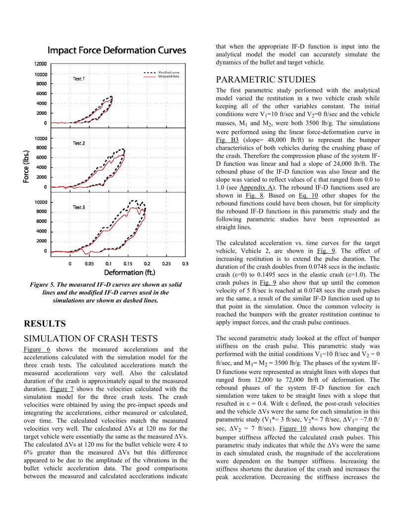
Figure 5. The measured IF-D curves are shown as solidlines and the modified IF-D curves used in the

simulations are shown as dashed lines.

RESULTSSIMULATION OF CRASH TESTSFigure 6 shows the measured accelerations and theaccelerations calculated with the simulation model for thethree crash tests. The calculated accelerations match themeasured accelerations very well. Also the calculatedduration of the crash is approximately equal to the measuredduration. Figure 7 shows the velocities calculated with thesimulation model for the three crash tests. The crashvelocities were obtained by using the pre-impact speeds andintegrating the accelerations, either measured or calculated,over time. The calculated velocities match the measuredvelocities very well. The calculated ΔVs at 120 ms for thetarget vehicle were essentially the same as the measured ΔVs.The calculated ΔVs at 120 ms for the bullet vehicle were 4 to6% greater than the measured ΔVs but this differenceappeared to be due to the amplitude of the vibrations in thebullet vehicle acceleration data. The good comparisonsbetween the measured and calculated accelerations indicate

that when the appropriate IF-D function is input into theanalytical model the model can accurately simulate thedynamics of the bullet and target vehicle.

PARAMETRIC STUDIESThe first parametric study performed with the analyticalmodel varied the restitution in a two vehicle crash whilekeeping all of the other variables constant. The initialconditions were V1=10 ft/sec and V2=0 ft/sec and the vehiclemasses, M1 and M2, were both 3500 lb/g. The simulationswere performed using the linear force-deformation curve inFig. B3 (slope= 48,000 lb/ft) to represent the bumpercharacteristics of both vehicles during the crushing phase ofthe crash. Therefore the compression phase of the system IF-D function was linear and had a slope of 24,000 lb/ft. Therebound phase of the IF-D function was also linear and theslope was varied to reflect values of ε that ranged from 0.0 to1.0 (see Appendix A). The rebound IF-D functions used areshown in Fig. 8. Based on Eq. 10 other shapes for therebound functions could have been chosen, but for simplicitythe rebound IF-D functions in this parametric study and thefollowing parametric studies have been represented asstraight lines.

The calculated acceleration vs. time curves for the targetvehicle, Vehicle 2, are shown in Fig. 9. The effect ofincreasing restitution is to extend the pulse duration. Theduration of the crash doubles from 0.0748 secs in the inelasticcrash (ε=0) to 0.1495 secs in the elastic crash (ε=1.0). Thecrash pulses in Fig. 9 also show that up until the commonvelocity of 5 ft/sec is reached at 0.0748 secs the crash pulsesare the same, a result of the similar IF-D function used up tothat point in the simulation. Once the common velocity isreached the bumpers with the greater restitution continue toapply impact forces, and the crash pulse continues.

The second parametric study looked at the effect of bumperstiffness on the crash pulse. This parametric study wasperformed with the initial conditions V1=10 ft/sec and V2 = 0ft/sec, and M1= M2 = 3500 lb/g. The phases of the system IF-D functions were represented as straight lines with slopes thatranged from 12,000 to 72,000 lb/ft of deformation. Therebound phases of the system IF-D function for eachsimulation were taken to be straight lines with a slope thatresulted in ε = 0.4. With ε defined, the post-crash velocitiesand the vehicle ΔVs were the same for each simulation in thisparametric study (V1*= 3 ft/sec, V2*= 7 ft/sec, ΔV1= −7.0 ft/sec, ΔV2 = 7 ft/sec). Figure 10 shows how changing thebumper stiffness affected the calculated crash pulses. Thisparametric study indicates that while the ΔVs were the samein each simulated crash, the magnitude of the accelerationswere dependent on the bumper stiffness. Increasing thestiffness shortens the duration of the crash and increases thepeak acceleration. Decreasing the stiffness increases the

duration of the crash pulse and decreases the peakacceleration.

Figure 6. The Acceleration vs. Time curves for the threecrash tests. The measured accelerations are solid linesand the accelerations calculated with the simulation

model are dashed lines. The accelerations for the bulletvehicle (Vehicle 1) are negative during the crash and the

accelerations for the target vehicle (Vehicle 2) arepositive.

Figure 7. The Velocity vs. Time curves for the threecrash tests. The velocities based on the measured

accelerations are shown as solid lines and the velocitiescalculated with the simulation model are shown as

dashed lines.

Figure 8. The rebound IF-D functions used in theparametric study where ε was varied. In these reboundcurves the deformation curve starts at maximum crush

(0.47 ft) and then moves to the left as the bumperstructures rebound.

Figure 9. The calculated Acceleration vs. Time curvesfor the target vehicle in crashes with different ε.

The third parametric study varied the closing speed and keptthe other parameters the same. Both vehicles had the samemass (M1=M2=3500lb/g) in this parametric study. Thecompression phase of the IF-D function was a straight linewith a slope of 24,000 lb/ft and the rebound phase was astraight line that represented an ε of 0.4 (see Fig. 8). Thecalculated crash pulses are shown in Fig.11. For a givenstiffness and the same relative amount of restitution theduration of the pulse was the same for the different closingspeeds. Increasing the closing speed increased the magnitudeof the accelerations produced in the crash, but it did notchange the duration of the pulse.

Figure 10. The calculated Acceleration vs. Time curvesfor the target vehicle in crashes with different bumper

stiffness.

Figure 11. The calculated Acceleration vs. Time curvesfor the target vehicle for different closing speeds.

TECHNIQUE TO ESTIMATE PEAKACCELERATIONOne of the applications of this numerical analytical model isto estimate the peak acceleration experienced by a vehicle ina low-speed bumper-to-bumper crash where there is little orno damage to the bumpers involved in the crash. There aretwo steps in this analysis. The first step is to measure theforce-deflection characteristics of the bumper systemsinvolved in the crash. Both bumper systems should becompressed until there is a structural failure of a componentof the bumper system, usually the impact bar. The damageproduced in the measurement of the force-deformationcharacteristics must be significantly greater than the damageto the bumper systems that were involved in the crash beinginvestigated. The lowest failure force represents an upperlimit to the peak impact force in the subject incident. Thesecond step is to perform simulations with the numericalmodel that determine what closing speed is required to createan impact force that is equal to or greater than the lowestfailure force. A system IF-D function can be created from themeasured force-deflection data. The simulations areperformed using the masses of the vehicles involved in the

actual crash. The simulations also provide the ΔVsexperienced by the vehicles. The crash severity estimatesobtained with this technique will provide an upper limit to theseverity of the crash being investigated.

The analysis presented is for a fictional crash where Vehicle2 is stationary and was rear-ended by Vehicle 1. Bothvehicles have the same mass (M1=M2=3500 lb/g). Thestructural characteristics of Vehicle 2's rear bumper arerepresented by the force-deformation curve for the Edgebumper shown in Fig. B3 and the structural characteristics ofVehicle 1's front bumper are represented by the force-deformation curve for a 2007 Kia Sportage's front bumper(see Fig. B4). The impact bar for the Sportage's front bumperfailed at a force of approximately 5000 lbs in the quasi-staticcompression tests. The force-deformation curve for bothbumpers has been approximated with the straight lines shownon the graphs in Figures B3 and B4 and the system IF-Dfunction (Eq. 11) is a straight line with a slope of 18,462 lb/ft.This line is shown as a solid line in Fig. B4.

If in the actual crash the plastic energy absorber of Vehicle 2was damaged but neither impact bar was deformed, then apeak closing speed and a peak acceleration can be estimatedby running the simulation model to find the impact speed forVehicle 1 that results in a peak impact force greater than5000 lb. In this case, the lack of damage to Vehicle 1's impactbar is being used to set an upper limit to the peak impactforce. In order to maximize the ΔV for the impact the valueof ε can be set high, although this will have no effect on thepeak acceleration or the peak impact force (see Fig. 9). Table3 shows the results of this iteration procedure with ε = 0.8.For this example the simulations indicate that if Vehicle 1 hitthe rear of Vehicle 2 at a speed of 5 ft/sec the peak impactforce would by 5009 lb and the impact bar in Vehicle 1 mayhave significant damage since this is just above the 5000 lbfailure limit for this bumper's impact bar. An impact speed of6 ft/sec would provide a more conservative estimate of themaximum impact speed and a better guarantee (taking intoaccount bumper-to-bumper differences) that Vehicle 1'simpact bar would fail. Since Vehicle 1's impact bar was notdamaged in the subject incident, an impact speed of 6ft/secprovides a conservative upper limit to the impact speed ofVehicle 1 in the subject crash.

TABLE 3. Calculated peak acceleration and forces fordifferent impact speeds of Vehicle1.

DISCUSSION AND CONCLUSIONSThe low-speed simulation model has been used to perform anumber of parametric studies in order to understand howdifferent variables affect the crash pulse in a low-speed crash.These parametric studies would be very difficult to replicatewith actual crash testing as it would be virtually impossible tohold all of the parameters constant in a series of real crasheswhile only one variable was changed. The low-speedsimulation model allows this type of analysis to be performedin a theoretical setting.

It is important to point out that the findings in theseparametric studies are not the result of the model but are adirect result of Newton's Laws being applied in the simulatedcrashes. The model presented here is not necessary to reachthe conclusions that are demonstrated in these parametricstudies, these same conclusions could have been reachedwithout the analytical model. The model is simply applyingNewton's Laws to crash scenarios where one variable ischanged in a series of simulated crashes. The model providesa tool to quantify and visualize how changing a singleparameter affects the vehicle dynamics in a crash.

The first parametric study looked at how ε affected the crashpulse. As ε was increased from 0 to 1.0 the duration of thecrash pulse doubled. Restitution affects the crash by allowingthe deformed structures to continue to apply forces after thecommon velocity is reached. When ε equals zero was therewas no rebound of the deformed structures and the crash wasover once the vehicles reached a common velocity. When εwas greater than zero the crash continued after the vehiclesreached a common velocity, albeit with a continuouslydecreasing impact force. Thus restitution does not change thepeak impact force or the peak acceleration, but it doesincrease the separation velocity and the ΔV experienced byeach vehicle in the crash. This same conclusion was reachedin the discussions of the IF-D curves shown in Figures A2and A3, but as described in the preceding paragraph, themodel provides a method of quantifying and demonstratingthe effect of changes in ε on the vehicle accelerations in acrash.

The second parametric study looked at how bumper stiffnessaffected the crash pulse. In this parametric analysis the ε forthe crash was kept constant by adjusting the rebound phase ofthe IF-D function (Fig. 8) and the pre-impact velocities werekept constant, therefore the ΔVs of Vehicle 1 and Vehicle 2were the same in each simulation of this parametric study.Increasing the stiffness of the bumpers increased the peakaccelerations and decreased the duration of the crash pulse asshown in Fig. 10.

The third parametric study kept all model variables constantexcept for the closing speed. This analysis produced theinteresting result that the pulse duration was a constant

regardless of the closing speed, and the accelerationsdecreased as the closing speed decreased (Fig. 11). Thisparametric study and the stiffness parametric study (Fig. 10)indicate that the stiffness of the bumper system determinesthe duration of the crash pulse for a given ε.

The analytical model was used to simulate three low-speedcrash tests in which the dynamic IF-D curve was created fromdata measured during the crash tests. In order to use thesedata a modification was required because, as shown in Fig. 4,the force and accelerometer data approximated Newton'sSecond Law throughout the crash, but did not follow itexactly. When a numerical simulation of a crash test wasperformed with the dynamic IF-D curve an error wasgenerated because the vehicles in the simulation had notreached a common velocity when maximum crush wasreached and the rebound phase of the crash should bestarting. The modification made to the measured IF-D datawas to simply multiply the measured force by a constant thatallowed the bullet and target vehicle to reach a commonvelocity in the simulation when the deformation reached themaximum deformation on the dynamic IF-D curve. Thismodification allowed the numerical simulations of the threecrashes to be completed and the calculated accelerations andvelocities were similar to the measured accelerations (Fig. 6)and velocities (Fig. 7). The accurate simulation of the threecrash tests indicates that the analytical model can recreate acrash given the appropriate IF-D function.

When the simulation model is being used to recreate thedynamics of a crash or put limits on a crash that has occurredthe accuracy of the calculated crash pulse depends on the IF-D function that is input into the model and how accuratelythis IF-D function represents the dynamic performance of thebumper systems involved in the actual crash event. Themeasured quasi-static force-deflection curves shown inFigures B3, B4 and B5 as solid lines were obtained with aconstant deformation rate and the bumpers were taken tofailure. The loading of the bumpers was done with a rigidsteel beam (Fig. B2). There was also a bumper systemcompression test performed by replacing the steel beam withthe rear bumper of a 2007 Kia Sportage and compressing a2007 Ford Edge front bumper up to a peak force ofapproximately 9500 lb (dashed line in Fig. B5). Anothersystem curve was made by adding the deformation in thequasi-static curves for the Edge's front bumper (Fig. B3) andthe Sportage's rear bumper together to create a system curvefor these two bumpers (dotted line in Fig. B5). Figure 12compares these two quasi-static system curves in Fig. B5with the measured IF-D curve in Test 3. The compressionphase of the system curve obtained with the two bumpersapproximates the measured IF-D curve better than the systemcurve made from the two separate quasi-static tests using thesteel beam. This one comparison indicates that the geometryof the object applying a force to a bumper in a compressiontest may be important in determining the system IF-D curve

and the quasi-static data that best represents the compressionphase of the dynamic IF-D curve may be obtained bymeasuring the quasi-static force-deformation characteristicsof the both bumpers together and not individually. This is anarea for future work.

Another area for future work is to determine if it is possibleto develop a method to accurately quantify the rebound phaseof the IF-D function based on quasi-static measurements. Asshown in Fig. 12 the quasi-static system IF-D curve (dashedline) accurately portrays the compression phase of themeasured IF-D curve but does not accurately portray therebound phase. It is important to have an accurate descriptionfor the rebound phase of the IF-D function because therebound curve determines what ε will be for the crash. Thedevelopment of a method to define the rebound curve willrequire comparisons between IF-D curves obtained quasi-statically and dynamically, i.e. through crash tests fordifferent bumper systems.

Figure 12. The dynamic IF-D curve measured in Test 3is shown as a solid line. The IF-D curve obtained from

the quasi-static compression tests with the beam is shownas the dotted line and the IF-D curve obtained by

compressing the two bumpers into each other is shownas a dashed line.

REFERENCES1. Thomson, R.W. and Romilly, D.P. “Simulation ofBumpers During Low Speed Impacts”, Proceeding of theCanadian Multidisciplinary Road Safety Conference III.Saskatoon, Saskatchewan, Canada, 1993.

2. Bailey, M.N., Wong, B.C., and Lawrence, J.M., “Data andMethods for Estimating the Severity of Minor Impacts,” SAETechnical Paper 950352, 1995.

3. Ojalvo, I.U. and Cohen, E.C.. “An Efficient Model forLow Speed Impacts of Vehicles,” SAE Technical Paper970779, 1997.

4. Ojalvo, I.U., Weber, B.E., Evensen, D.A., Szabo, T.J. etal., “Low Speed Car Impacts with Different Bumper Systems:Correlation of Analytical Model with Tests,” SAE TechnicalPaper 980365, 1998.

5. Cipriani, A.L., Bayan, F.P., Woodhouse, M.L., Cornetto,A.D. et al., “Low Speed Collinear Impact Severity: AComparison between Full Scale Testing and AnalyticalPrediction Tools with Restitution Analysis,” SAE TechnicalPaper 2002-01-0540, 2002.

6. Happer, A.J., Hughes, M.C., Peck, M.D., and Boehme,S.M., “Practical Analysis Methodology for Low SpeedVehicle Collisions Involving Vehicles with Modern BumperSystems,” SAE Technical Paper 2003-01-0492, 2003.

7. Brach, R.M., “Model of Low-Speed, Front-to-RearVehicle Impacts,” SAE Technical Paper 2003-01-0491, 2003.

8. Collins, J.C. “Accident Reconstruction”, Charles C.Thomas, Springfield, Illinois, USA, 1979.

9. 2008 Mitchell Collision Estimating & Reference Guide,Mitchell International, 9889 Willow Creek Road, San Diego,CA.

CONTACT INFORMATIONWilliam R. “Mike” ScottBiodynamic Research Corporation5711 University Heights Blvd., Suite 100San Antonio, Texas 78249Phone: (210) 691-0281Fax: (210) 691-8823mscott@brconline.com

A copy of the Matlab7 code used in the parametric studieswill be e-mailed upon request.

ACKNOWLEDGMENTSThe authors acknowledge the work of Mr. Enrique Bonugliand Mr. Herb Guzman for performing the quasi-staticmeasurements on the bumper systems presented in this paperand for performing the crash tests. The authors also thank Mr.Jimmy Cosgrove and Mr. Bob Carlin for creating theillustrations.

The authors would also like to thank the reviewers for theircomments and suggestions as well as for the time that theyspend reviewing this manuscript.

APPENDIX A

ENERGY DEFINITION OF THECOEFFICIENT OF RESTITUTIONA two vehicle system composed of Vehicle 1 and Vehicle 2has a common center of mass that is located between the twovehicles and moves with the vehicles. If the masses ofVehicle 1 and Vehicle 2 are M1 and M2, then the mass of thecommon center of mass is M1+M2. If the velocity of Vehicle1 and Vehicle 2 are V1 and V2 then the velocity of thecommon center of mass (Vcm) is,

(1A)

In a crash Vcm does not change because of conservation ofmomentum. The common center of mass also has a kineticenergy (KE) associated with it,

(2A)

Since Vcm does not change in a crash, Ecm also does notchange. The system of two vehicles also has a pre-crash KEwhich is the sum of the KE of each vehicle,

(3A)

The KE of the system is greater than Ecm and the differenceis Eafc,

(4A)

where Eafc is the amount of energy available for crush and forheat generation in the two car system pre-crash (8). For thisanalysis it is assumed that the heat generated in a crash isnegligible and it is neglected. Usually only some of Eafc isused up in a crash and after the vehicles separate there is stillsome energy, Eafc*, in the system that can be used for crush.If the post-crash velocities of Vehicle 1 and Vehicle 2 areV1* and V2*, then

(5A)

The energy definition of the coefficient of restitution is ε2

equals the fraction of Eafc that was not used in the crash tocreate heat or crush metal (8), and

(6A)

When Eqs. 4A and 5A are substituted into Eq. 6A for Eafc*and Eafc, the result is Eq. 9. Eq. 9 describes the effect ofrestitution on post-crash velocities. Eq. 6A describes how theenergy balance in the system is influenced by the restitutionin the crash.

Figure A1 graphically shows the kinetic energy allocation ina collinear two vehicle system before and after a crash. In thissystem Vehicle 2 is initially stationary (V2=0) and Vehicle 1impacts the rear of Vehicle 2 with velocity V1. The masses ofVehicle 1 and 2 are taken to be equal. Prior to the crash, Esys

= ½M1V12 (Eq. 3A). One half of the system KE is in the

center of mass motion, Ecm = ¼ M1V12 (Eq. 2A), and the

other half of

Figure A1. The kinetic energy distribution in a twovehicle system before the crash and after the crash.

the system KE is available for crush, Eafc = ¼ M1V12 (Eq.

4A). Post-crash Ecm has not changed, but the energy availablefor crush in a subsequent impact, Eafc*, has decreased. Theratio between the amount of energy available for crush post-crash (Eafc*) to the amount available pre-crash (Eafc) is equalto ε2 as described in Eq. 6A (8). The lost KE has gone intothe work of crushing the vehicle bumper systems.

The energy definition for ε indicates that the force-deformation characteristics of the vehicles structures thatmake contact in the crash determine ε for that crash. TheImpact Force-Deformation curves in Figs. A2 and A3illustrate this concept in two crashes. Deformation is made upof crush, which is permanent and elastic deformation. Thedeformation in Figs. A2 and A3 represents the sum of thedeformation of both vehicles at a given impact force. Fig. A2represents a crash where most of the deformation ispermanent crush and Fig. A3 represents a crash with the same

initial conditions but the majority of the deformation iselastic. Once the vehicles make contact the structures willdeform and an impact force will be created that acts on bothvehicles. If the impact force and deformation at a given timein the crash are plotted on the Impact Force vs. Deformationcoordinate system the points will form a curve that movesover the plane of the coordinate system with time. As long asthe deformation continues to increase the Impact Force-Deformation curve will move to the right on

Figure A2. The impact force-deformation curve for acrash where there is little rebound of the bumper

structures during the crash. Eafc is the area under theupper curve from 0 to Dmax. Eafc* is the shaded area.

the diagram. The Impact Force-Deformation curve willcontinue to the right until the vehicles reach a commonvelocity and the deformation is at a maximum (Dmax). Sinceboth vehicles have the same velocity at this point in the crash,they are in a situation, at least temporarily, where ε =0, andall of Eafc has been used up to create the deformation up toDmax. Therefore, the area under the Impact Force-Deformation curve up to Dmax must equal Eafc. In high speedcrashes or crashes where the vehicles have inelastic structuresthis is the end of the crash, ε is approximately zero and theimpacting vehicles depart the crash with similar velocities.This situation is depicted in Fig. A2 where the Impact Force-Deformation curve after Dmax has a steep slope and thepermanent crush, Dperm, is just slightly less than Dmax. In thissituation almost all of the energy available for crush, Eafc, hasbeen used to crush the two vehicles and ε2≈ 0.

The situation is very different when the deformed structuresare more elastic because the crash is not over once thevehicles reach a common velocity. Fig. A3 illustrates thesame crash as shown in Fig. A2 except that the deformedstructures are more elastic. The path up to Dmax is the sameas in Figure A2, but after Dmax is reached the deformedstructures rebound a significant amount and the permanentcrush is a fraction of the maximum deformation. The work

done by the rebounding structures is Eafc* and this energy isreturned to the system. This returned energy increases theseparation velocity (V1*−V2*), the system kinetic energy andthe ΔV experienced by each vehicle in the crash.

Figure A3. The impact force-deformation curve for acrash where there is significant rebound of the bumperstructures during the crash. Eafc is the area under theupper curve from 0 to Dmax. Eafc* is the shaded area.

APPENDIX B

DESCRIPTION OF THE BUMPERSUSED IN THE CRASH TESTS ANDSIMULATIONSStatic-force deflection measurements were made on threebumpers for this study. The three bumpers are the frontbumper of the 2007 Ford Edge and the front and rear bumperof the 2007 Kia Sportage. Schematics for the three bumpersare shown in Fig. B1 (9).

The Edge front bumper is constructed of a curved metalimpact bar with a honeycomb plastic energy absorber placedbetween the impact bar and the plastic cover as shown in Fig.B1. The Sportage's front bumper has a metal impact bar withno energy absorbing element between the impact bar and thecover, as shown in Figure B2. The Sportage's rear bumperhas a curved composite impact bar with a cover. There is anenergy absorbing foam material on the top of the impact bar,but this foam material only covered approximately the top 1.5inches of the rear surface of the impact bar. This foamappears to be designed as a vertical support for the bumpercover so that people can step on or place objects on the top ofthe rear bumper.

2007 Ford Edge Front Bumper

2007 Kia Sportage Front Bumper

2007 Kia Sportage Rear BumperFigure B1. Schematics of the bumpers used in this study.

The static force-deformation characteristics of the bumperswere measured by mounting the bumper onto a rigid baseusing the same brackets that are used to attach the bumper tothe vehicle body. The center of the test bumper wascompressed by a beam that had a curved surface similar to abumper's shape and a width of 2.5 inches. The beam wasattached to a hydraulic piston. The rate of compression was

approximately 0.075 ft/sec. The compression force wasmeasured with a load cell attached to the top of the beam(Model 1210A-25k, Interface Corp.) and the displacementwas measured with a displacement transducer (LVDT type,LH series, MTS, Inc.). Figure B2 shows the shape of the steelbeam used to compress the bumpers along with the Edge'simpact bar and honeycomb energy absorber without thebumper cover. The load cell is mounted directly over thisbeam.

Figure B2. Photograph of the test setup used to measurethe force-deformation characteristics of the bumpers.

Figure B3 shows the quasi-static force-deformation curvemeasured on a new 2007 Ford Edge front bumper. Thebumper was compressed until the impact bar failed. The first0.021 ft of deformation in the compression phase of the curverepresents the crush of the plastic energy absorber. The slopeof the force-deformation curve increased after the plasticenergy absorber was crushed. The force increased untilapproximately 22,000 lbs when the impact bar failed andfurther compression resulted in a decrease in the force. Thedashed straight line (slope = 48,000 lb/ft) in Fig. B3approximates the compression phase of the force-deformationcurve of the Edge's bumper. The solid straight line (slope =24,000 lb/ft) in Fig. B3 represents a system IF-D function ofa bumper system that is composed of two bumpers that havea linear stiffness of 48,000 lb/ft (Eq. 11).

Figure B4 shows the quasi-static force-deformation curvemeasured on a new 2007 Kia Sportage front bumper. Theimpact bar completely failed at a force of approximately 5000lb. The compression part of the force-deformation curve inFig. B4 has been approximated with a line that has a slope of30,000 lb/ft. When this linear force-deformation curve iscombined with the linear force-deformation curve for theEdge (48,000 lb/ft) the system IF-D function (Eq. 11) is astraight line with a slope of 18,462 lb/ft. This IF-D function isshown as a solid straight line in Fig. B4.

Figure B5 shows the quasi-static force-deformation curvemeasured with a new 2007 Kia Sportage rear bumper as asolid line. This test was performed without the foam energyabsorber that covered the top rear surface of the impact barbecause the discontinuity in the surface could have produceda bending moment that may have damaged the load cell. Theforce increased until it reached approximately 17,500 lbswhen there was a load noise and the composite impact barcracked. The dotted line in Fig. B5 is a system compressionIF-D function made by adding the deformation in thecompression phase of the force-deformation curve for theEdge's front bumper and the Kia Sportage's rear bumper forforces up to 10,000 lb. There is no data available from ourmeasurements to construct a rebound phase for this systemIF-D function so only the compression phase is shown.Another system IF-D curve was produced by replacing thecompression beam shown in Fig. B2 with a new Kia Sportagerear bumper and using this bumper to compress a new FordEdge front bumper. The two bumpers were compressed up toapproximately 9,600 lbs and then the force was released. Thesystem force-deformation curve measured in this test isshown in Fig B5 as a dashed line. The quasi-static force-deformation curve obtained with the two bumpers is stifferthan the curve obtained by combing the two quasi-static tests.The difference appears to reflect the geometrical differencebetween the steel bar and the Sportage's rear bumper. Thesteel bar is narrower and has a smaller contact area than theSportage's rear bumper. The reduced contact area may allowthe beam to crush the honeycomb plastic at a lower force thanthe Sportage's bumper.

Figure B3. The quasi-static Force-Deformation curve forthe Edge's front bumper. The dashed line is a linearapproximation of the upper part of the curve and the

solid line represents the compression phase of a systemIF-D function for a simulation where both bumpers have

the stiffness defined by the dashed line.

Figure B4. The quasi-static Force-Deformation curve forthe Sportage's front bumper. The dotted line is a linearapproximation of the upper part of the curve and the

solid line represents the compression phase of a systemIF-D function that has a stiffness of 18,462 lb/ft.

Figure B5. The quasi-static Force-Deformation curve forthe Sportage's rear bumper is shown as a solid line. The

dotted line is the quasi-static compression Force-Deformation curve made by combining the curve for the

Edge's front bumper and the Sportage's rear bumper.The dashed line is the measured quasi-static Force-

Deformation curve obtained by compressing theSportage's rear bumper into the Edge's front bumper.

The Engineering Meetings Board has approved this paper for publication. It hassuccessfully completed SAE's peer review process under the supervision of the sessionorganizer. This process requires a minimum of three (3) reviews by industry experts.

All rights reserved. No part of this publication may be reproduced, stored in aretrieval system, or transmitted, in any form or by any means, electronic, mechanical,photocopying, recording, or otherwise, without the prior written permission of SAE.

ISSN 0148-7191

doi:10.4271/2010-01-0051

Positions and opinions advanced in this paper are those of the author(s) and notnecessarily those of SAE. The author is solely responsible for the content of the paper.

SAE Customer Service:Tel: 877-606-7323 (inside USA and Canada)Tel: 724-776-4970 (outside USA)Fax: 724-776-0790Email: CustomerService@sae.orgSAE Web Address: http://www.sae.orgPrinted in USA