thorsten rheinlander and gallus steiger the minimal...
TRANSCRIPT

Thorsten Rheinlander and Gallus Steiger The minimal entropy martingale measure for general Barndorff-Nielsen/Shephard models Article (Published version) (Refereed)
Original citation: Rheinlander, Thorsten and Steiger, Gallus (2006) The minimal entropy martingale measure for general Barndorff-Nielsen/Shephard models. Annals of applied probability, 16 (3). pp. 1319-1351. ISSN 1050-5164 DOI: 10.1214/105051606000000240 © 2006 IMS This version available at: http://eprints.lse.ac.uk/16351/ Available in LSE Research Online: December 2011 LSE has developed LSE Research Online so that users may access research output of the School. Copyright © and Moral Rights for the papers on this site are retained by the individual authors and/or other copyright owners. Users may download and/or print one copy of any article(s) in LSE Research Online to facilitate their private study or for non-commercial research. You may not engage in further distribution of the material or use it for any profit-making activities or any commercial gain. You may freely distribute the URL (http://eprints.lse.ac.uk) of the LSE Research Online website.

The Annals of Applied Probability2006, Vol. 16, No. 3, 1319–1351DOI: 10.1214/105051606000000240© Institute of Mathematical Statistics, 2006
THE MINIMAL ENTROPY MARTINGALE MEASURE FORGENERAL BARNDORFF-NIELSEN/SHEPHARD MODELS1
BY THORSTEN RHEINLÄNDER AND GALLUS STEIGER
London School of Economics and ETH Zürich
We determine the minimal entropy martingale measure for a generalclass of stochastic volatility models where both price process and volatilityprocess contain jump terms which are correlated. This generalizes previousstudies which have treated either the geometric Lévy case or continuous priceprocesses with an orthogonal volatility process. We proceed by linking theentropy measure to a certain semi-linear integro-PDE for which we prove theexistence of a classical solution.
1. Introduction. The main contribution of this paper is the calculation of theminimal entropy martingale measure (MEMM) for a general class of stochasticvolatility models as explicitly as possible in terms of the parameters of the marketmodel. This idea of explicit description of optimal martingale measures startedwith the minimal martingale measure of Föllmer and Schweizer [12], followedby the minimal Hellinger martingale measure of Grandits [15] and the minimalentropy-Hellinger martingale measure of Choulli and Stricker [8].
Our study of the MEMM encompasses the simpler cases where either the dy-namics of the risky asset is modeled as a geometric Lévy process or the priceprocess is continuous with an orthogonal pure jump volatility process. These cases,as will be discussed below, have been studied separately and with different meth-ods. Our approach presents a unifying framework which moreover covers modelslike the Barndorff-Nielsen and Shephard (BN–S) model where both price processand volatility process contain jump terms which are correlated. It turns out that,due to the correlation, this general case is much more difficult and can be consid-ered a nontrivial mixture of the two cases studied previously.
Asset process models driven by nonnormal Lévy processes date back to thework of Mandelbrot [22]. More recently, rather complex models like the stochas-tic volatility model of Barndorff-Nielsen and Shephard [1] have been developed.This model is constructed via a jump-diffusion price process together with a meanreverting, stationary volatility process of Ornstein–Uhlenbeck type driven by asubordinator (i.e., an increasing Lévy process). Moreover, the negative correlationbetween price process and volatility process in this model allows us to deal with
Received March 2005; revised November 2005.1Supported by NCCR Financial Valuation and Risk Management.AMS 2000 subject classifications. 28D20, 60G48, 60H05, 91B28.Key words and phrases. Relative entropy, martingale measures, stochastic volatility.
1319
1320 T. RHEINLÄNDER AND G. STEIGER
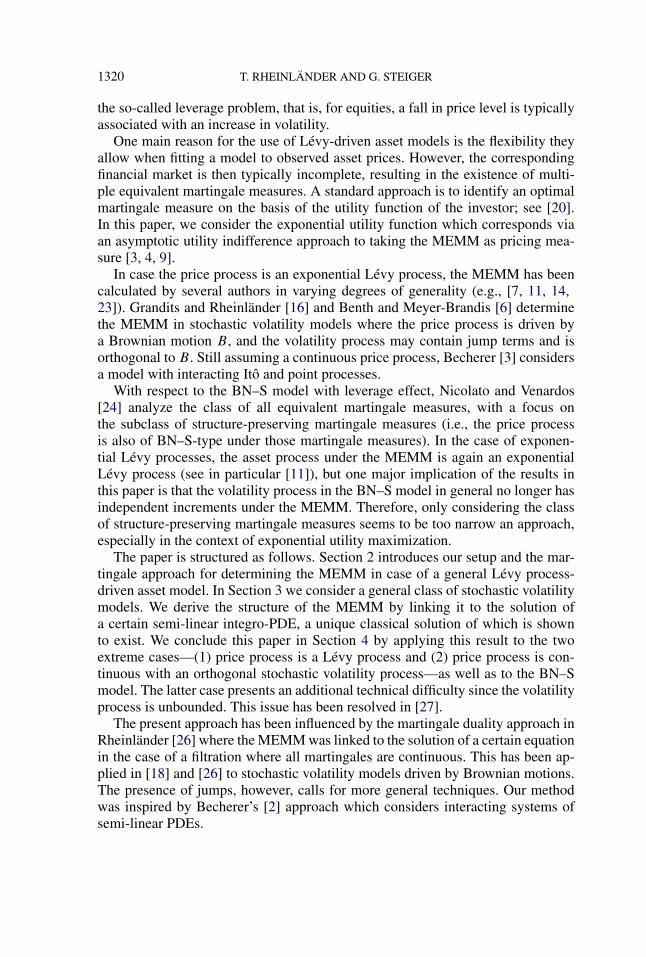
the so-called leverage problem, that is, for equities, a fall in price level is typicallyassociated with an increase in volatility.
One main reason for the use of Lévy-driven asset models is the flexibility theyallow when fitting a model to observed asset prices. However, the correspondingfinancial market is then typically incomplete, resulting in the existence of multi-ple equivalent martingale measures. A standard approach is to identify an optimalmartingale measure on the basis of the utility function of the investor; see [20].In this paper, we consider the exponential utility function which corresponds viaan asymptotic utility indifference approach to taking the MEMM as pricing mea-sure [3, 4, 9].
In case the price process is an exponential Lévy process, the MEMM has beencalculated by several authors in varying degrees of generality (e.g., [7, 11, 14,23]). Grandits and Rheinländer [16] and Benth and Meyer-Brandis [6] determinethe MEMM in stochastic volatility models where the price process is driven bya Brownian motion B , and the volatility process may contain jump terms and isorthogonal to B . Still assuming a continuous price process, Becherer [3] considersa model with interacting Itô and point processes.
With respect to the BN–S model with leverage effect, Nicolato and Venardos[24] analyze the class of all equivalent martingale measures, with a focus onthe subclass of structure-preserving martingale measures (i.e., the price processis also of BN–S-type under those martingale measures). In the case of exponen-tial Lévy processes, the asset process under the MEMM is again an exponentialLévy process (see in particular [11]), but one major implication of the results inthis paper is that the volatility process in the BN–S model in general no longer hasindependent increments under the MEMM. Therefore, only considering the classof structure-preserving martingale measures seems to be too narrow an approach,especially in the context of exponential utility maximization.
The paper is structured as follows. Section 2 introduces our setup and the mar-tingale approach for determining the MEMM in case of a general Lévy process-driven asset model. In Section 3 we consider a general class of stochastic volatilitymodels. We derive the structure of the MEMM by linking it to the solution ofa certain semi-linear integro-PDE, a unique classical solution of which is shownto exist. We conclude this paper in Section 4 by applying this result to the twoextreme cases—(1) price process is a Lévy process and (2) price process is con-tinuous with an orthogonal stochastic volatility process—as well as to the BN–Smodel. The latter case presents an additional technical difficulty since the volatilityprocess is unbounded. This issue has been resolved in [27].
The present approach has been influenced by the martingale duality approach inRheinländer [26] where the MEMM was linked to the solution of a certain equationin the case of a filtration where all martingales are continuous. This has been ap-plied in [18] and [26] to stochastic volatility models driven by Brownian motions.The presence of jumps, however, calls for more general techniques. Our methodwas inspired by Becherer’s [2] approach which considers interacting systems ofsemi-linear PDEs.

THE MINIMAL ENTROPY MARTINGALE MEASURE 1321
2. Preliminaries and general results. We start with some general assump-tions which hold throughout the paper. Let (�,F ,F,P ) be a filtered probabilityspace and T some fixed finite time horizon. We assume that F0 is trivial and thatF = F T . The filtration F = (Ft )0≤t≤T fulfills the usual conditions and is gener-ated by a Lévy process Y where Y c (Yd ), µY , and νY (dx, dt) = ν(dx) dt denoteits continuous (discontinuous) martingale part, the jump measure and its compen-sator, respectively. For simplicity, we assume that 〈Y c〉t = t . We refer to [19] withrespect to the notation used in this paper. In particular, Gloc(µY ) is defined in [19],Definition II.1.27.
REMARK 2.1. By Jacod and Shiryaev [19], Theorem III.4.34, we have thefollowing representation property: every (P,F)-local martingale M can be writtenas
M = M0 +∫
H dYc + W ∗ (µY − νY )
for some H ∈ L2loc(Y
c), W ∈ Gloc(µY ).
We denote by S an F-adapted, locally bounded semimartingale (modeling theprice process of a risky asset), which has the following canonical decomposition:
S = S0 + M + A,
where M is a locally bounded local martingale with M0 = 0 and A is a process oflocally finite variation. By the representation property, we write M as
M = Mc + Md =∫
σM dY c + WM(x) ∗ (µY − νY ),
where Mc and Md are the continuous and the discontinuous parts of the localmartingale M , respectively, σM is predictable and WM ∈ Gloc(µY ). Moreover, weassume that the asset price process S satisfies the following:
ASSUMPTION 2.2 (Structure condition). There exists a predictable process λ
satisfying
A =∫
λd〈M〉,with
KT :=∫ T
0λ2
s d〈M〉s < ∞, P -a.s.
DEFINITION 2.3. Let V be the linear subspace of L∞(�,F ,P ) spanned bythe elementary stochastic integrals of the form f = h(ST2 − ST1), where 0 ≤ T1 ≤T2 ≤ T are stopping times such that the stopped process ST2 is bounded and h is abounded FT1 -measurable random variable. A martingale measure is a probabilitymeasure Q � P with E[dQ
dPf ] = 0 for all f ∈ V .

1322 T. RHEINLÄNDER AND G. STEIGER
We denote by M the set of all martingale measures for S and by Me the subsetof M consisting of probability measures which are equivalent to P . Here and inthe sequel, we identify measures with their densities. Note that, as S is locallybounded, a probability measure Q absolutely continuous to P is in M if and onlyif S is a local Q-martingale.
DEFINITION 2.4. The relative entropy I (Q,R) of the probability measure Q
with respect to the probability measure R is defined as
I (Q,R) =ER
[dQ
dRlog
dQ
dR
], if Q � R,
+∞, otherwise.
It is well known that I (Q,R) ≥ 0 and that I (Q,R) = 0 if and only if Q = R.
DEFINITION 2.5. The minimal entropy martingale measure QE , also abbre-viated MEMM in what follows, is the solution of
minQ∈M
I (Q,P ).
Theorems 1, 2 and Remark 1 of [13], as well as the fact that V ⊂ L∞(P ), yieldthe following:
THEOREM 2.6 ([13]). If there exists Q ∈ Me such that I (Q,P ) < ∞, then theminimal entropy martingale measure exists, is unique and moreover is equivalentto P .
Let us restate the following criterion for a martingale measure to coincide withthe MEMM:
THEOREM 2.7 ([16]). Assume there exists a Q ∈ Me with I (Q,P ) < ∞.Then Q∗ is the minimal entropy martingale measure if and only if there existsa constant c and an S-integrable predictable process φ
dQ∗
dP= exp
(c +
∫ T
0φt dSt
)(2.1)
such that EQ[∫ T0 φt dSt ] = 0 for all Q ∈ Me with finite relative entropy.
REMARK 2.8. Based on the above results, we will pursue the following strat-egy to determine the MEMM. We first find some candidate measure Q∗ which canbe represented as in (2.1). To verify that Q∗ is indeed the entropy minimizer, wethen proceed in three steps, showing that:
1. Q∗ is an equivalent martingale measure;

THE MINIMAL ENTROPY MARTINGALE MEASURE 1323
2. I (Q∗,P ) < ∞;3.
∫φ dS is a true Q-martingale for all Q ∈ Me with finite relative entropy.
This martingale approach yields a necessary equation for φ and c:
THEOREM 2.9. Assume that the MEMM Q∗ exists. The strategy φ and theconstant c in (2.1) satisfy the equation
c +∫ T
0
[12(σL
t − λtσMt )2 + φtλt (σ
Mt )2 + φtλt
∫R
(WMt (x))2ν(dx)
]dt
=∫ T
0
(σL
t − (φt + λt )σMt
)dY c
t
(2.2)+ ((
WL(x) − (φ + λ)WM(x)) ∗ (µY − νY )
)T
+ ((log
(1 − λWM(x) + WL(x)
) + λWM(x) − WL(x)) ∗ µY
)T
with predictable processes σL ∈ L2loc(Y
c) and WL ∈ Gloc(µY ) such that
σMt σL
t +∫
R
WMt (x)WL
t (x)ν(dx) = 0 ∀ t ∈ [0, T ].(2.3)
PROOF. By Girsanov’s theorem together with the structure condition, the den-sity process Z = (Zt ) of Q∗ is a stochastic exponential of the form
Z = E
(−
∫λdM + L
),
where L and [M,L] are local P -martingales. Using the representation property,let us write the local martingale L in the following way:
L =∫
σL dY c + WL(x) ∗ (µY − νY ),(2.4)
for some σL ∈ L2loc(Y
c), WL ∈ Gloc(µY ). We therefore get
[M,L] =∫ ·
0σM
s σLs ds + WM(x)WL(x) ∗ µY .
Furthermore, we know from [10], VII.39, that the predictable bracket process
〈M,L〉 =∫ ·
0σM
s σLs ds + WM(x)WL(x) ∗ νY
exists, since M is locally bounded. However, 〈M,L〉 is equal to zero since [M,L]is a local martingale. Therefore, condition (2.3) holds. We now apply Itô’s formula

1324 T. RHEINLÄNDER AND G. STEIGER
to logZ to get, for t ∈ [0, T ], that
logZt =∫ t
0
1
Zs−dZs − 1
2
∫ t
0
1
Z2s−
d〈Zc〉s
+ ∑s≤t
(logZs − logZs− − 1
Zs−�Zs
)
= −∫ t
0λs dMs + Lt − 1
2
∫ t
0λ2
s d〈Mc〉s +∫ t
0λs d〈Mc,Lc〉s − 1
2〈Lc〉t
+ ∑s≤t
(log
Zs
Zs−+ �
∫ s
0λdM − �Ls
)
=∫ t
0(σL
s − λsσMs ) dY c
s − 1
2
∫ t
0(λsσ
Ms − σL
s )2 ds
+ ((WL(x) − λWM(x)
) ∗ (µY − νY ))t
+ ((log
(1 − λWM(x) + WL(x)
) + λWM(x) − WL(x)) ∗ µY
)t .
Moreover, due to Theorem 2.7, at the time horizon we have
logZT = c +∫ T
0φt dSt
= c +∫ T
0φtσ
Mt dY c
t + (φWM(x) ∗ (µY − νY )
)T
+∫ T
0
(φtλt (σ
Mt )2 + φtλt
∫R
(WMt (x))2ν(dx)
)dt.
We arrive at equation (2.2) by combining the two equations above. �
COROLLARY 2.10. Equation (2.2) in Theorem 2.9 is fulfilled once the follow-ing conditions are satisfied:
(i) |WL(x) − (φ + λ)WM(x)| ∗ µY ∈ A+loc.
(ii) It holds that
c +∫ T
0
[12(σL
t − λtσMt )2 + φtλt (σ
Mt )2]
dt
+∫ T
0
∫R
(WL
t (x) − (φt + λt )WMt (x) + φtλt (W
Mt (x))2)
ν(dx) dt
(2.5)
=∫ T
0
(σL
t − (φt + λt )σMt
)dY c
t
+ ((log
(1 − λWM(x) + WL(x)
) − φWM(x)) ∗ µY
)T .

THE MINIMAL ENTROPY MARTINGALE MEASURE 1325
PROOF. By Jacod and Shiryaev [19], Proposition II.1.28, condition (i) impliesthat we can write(
WL(x) − (φ + λ)WM(x)) ∗ (µY − νY ) = (
WL(x) − (φ + λ)WM(x)) ∗ µY
− (WL(x) − (φ + λ)WM(x)
) ∗ νY .
Taking this into account, equation (2.2) reduces to the simpler equation (2.5).�
Once we have, by solving (2.2) and (2.3), found a candidate martingale mea-sure, we still have to carry out the verification procedure outlined above. We willneed the following lemma, which is a generalization of the Novikov condition todiscontinuous processes:
LEMMA 2.11 ([21]). Let N be a locally bounded local P -martingale. LetQ be a measure defined by
dQ
dP
∣∣∣∣Ft
= Zt = E(N)t ,
where �N > −1. If the process
Ut = 12〈Nc〉t + ∑
s≤t
{(1 + �Ns) log(1 + �Ns) − �Ns}(2.6)
belongs to Aloc, and therefore has a predictable compensator Bt and, in addition,
E[expBT ] < ∞,(2.7)
then Q is an equivalent probability measure.
Finally, to cope with item 3 of our approach described in Remark 2.8, we men-tion the following result:
LEMMA 2.12 ([26]). Let Q be an equivalent martingale measure with fi-nite relative entropy, and let
∫ψ dS be a local Q-martingale. Then
∫ψ dS is
a true Q-martingale if, for some β > 0 small enough, exp{β ∫ T0 ψ2
t d[S]t } isP -integrable.
3. A general jump-diffusion model. Let us consider a class of stochasticvolatility models with asset prices of the following type:
dSt
St−= ηM(t,Vt ) dt + σM(t,Vt ) dY c
t + d(WM( · ,V−, x) ∗ (µY − νY )
)t ,(3.1)
dVt = ηV (t,Vt ) dt + d(WV ( · ,V−, x) ∗ µY
)t ,(3.2)
where V is defined on some interval E ⊂ R. In the notation we will often sup-press the dependence on V of the various processes. Our basic assumptions are asfollows:
1326 T. RHEINLÄNDER AND G. STEIGER
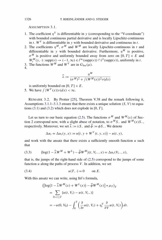
ASSUMPTION 3.1.
1. The coefficient ηV is differentiable in y (corresponding to the “V-coordinate”)with bounded continuous partial derivative and is locally Lipschitz-continuousin t . WV is differentiable in y with bounded derivative and continuous in t .
2. The coefficients ηM , σM and WM are locally Lipschitz-continuous in t anddifferentiable in y with bounded derivative. Furthermore, ηM is positive,σM is positive and uniformly bounded away from zero on [0, T ] × E andWM
t (y, ·) : supp(ν) → (−1,∞) ∈ l∞(supp(ν)) ∩ l1(supp(ν)), uniformly in t .3. The functions WM and WV are in Gloc(µ).4.
λ := ηM
(σM)2 + ∫(WM(x))2ν(dx)
is uniformly bounded on [0, T ] × E.5. We have
∫ |WV (x)|ν(dx) < ∞.
REMARK 3.2. By Protter [25], Theorem V.38 and the remark following it,Assumptions 3.1.1–3.1.3 ensure that there exists a unique solution (S,V ) to equa-tions (3.1) and (3.2) which does not explode in [0, T ].
Let us turn to our basic equation (2.5). The functions σM and WM(x) of Sec-tion 2 correspond now, with a slight abuse of notation, to σMS− and WM(x)S−,respectively. Moreover, we set λ := λS− and φ := φS−. We denote
�ut = �ut(y, x) := u(t, y + WV (t, y, x)
) − u(t, y),
and work with the ansatz that there exists a sufficiently smooth function u suchthat (
log(1 − λWM + WL) − φWM)(t,Vt−, x) = �ut(Vt−, x),(3.3)
that is, the jumps of the right-hand side of (2.5) correspond to the jumps of somefunction u along the paths of process V . In addition, we set
u(T , ·) = 0 on E.(3.4)
With this ansatz we can write, using Itô’s formula,([log
(1 − λWM(x) + WL(x)
) − φWM(x)] ∗ µY
)T
= ∑0<t≤T
{u(t,Vt ) − u(t,Vt−)}
= −u(0,V0) −∫ T
0
(∂
∂tu(t,Vt ) + ηV
t
∂
∂Vu(t,Vt )
)dt.

THE MINIMAL ENTROPY MARTINGALE MEASURE 1327
We may therefore rewrite equation (2.5) as
c + u(0,V0)
= −∫ T
0
[1
2(σL
t − λtσMt )2 + φt λt (σ
Mt )2
+ ∂
∂tu(t,Vt ) + ηV
t
∂
∂Vu(t,Vt )(3.5)
+∫ (
WLt (x) − (φt + λt )W
Mt (x) + φt λt (W
Mt (x))2)
ν(dx)
]dt
+∫ T
0[σL
t − (φt + λt )σMt ]dY c
t .
A solution to this problem might be to require that
1
2(σL − λσM)2 + φλ(σM)2 + ∂
∂tu(·,V ) + ηV ∂
∂Vu(·,V )
(3.6)+
∫ (WL(x) − (φ + λ)WM(x) + φλ(WM(x))2)
ν(dx) = 0,
together with (3.4) and
c = −u(0,V0), σL = (φ + λ)σM.(3.7)
Let us introduce ut := u(t, ·) :E → R and
gy(t, ut ) := 12
(σL
t (y) − λt (y)σMt (y)
)2 + φt (y)λt (y)(σMt (y))2
+∫ (
WLt (y, x) − (
φt (y) + λt (y))WM
t (y, x)(3.8)
+ φt (y)λt (y)(WM
t (y, x))2)
ν(dx).
Provided that φt , σLt and WL
t (x) are functions of ut , (3.6) is an integro-PDE for u
of the form∂
∂tu(t, y) + ηV
t
∂
∂yu(t, y) + gy(t, ut ) = 0,(3.9)
u(T , y) = 0 for all y ∈ E.(3.10)
By equation (3.7) together with condition (2.3), we get
φ = −λ −∫
WM(x)WL(x)ν(dx)
(σM)2 ,(3.11)
which, by equation (3.3), leads to (suppressing the t and y variables)
exp{�u(x) −
[λ +
∫WM(z)WL(z)ν(dz)
(σM)2
]WM(x)
}(3.12)
= 1 − λWM(x) + WL(x).

1328 T. RHEINLÄNDER AND G. STEIGER
To make this intuitive approach rigorous, we shall proceed as follows. Weshow in Corollary 3.4 below that each u ∈ Cb([0, T ] × E) gives via �u a uniquebounded function WL solving (3.12). We then define φ as in (3.11), σL as in (3.7)and gy as in (3.8). In Theorem 3.8 below it is then shown that there exists a clas-sical solution to the integro-PDE (3.9), (3.10). Finally, we provide the verificationresults in Theorem 3.9.
For the discussion of equation (3.12) we first provide a preparatory result:
LEMMA 3.3. Let β > 0, f ∈ l∞(supp(ν)) ∩ l1(supp(ν)), the set of boundedand integrable functions from supp(ν) into R, and k be a function on supp(ν)
which is bounded from above. Then, the function ϕ : supp(ν) → R, given as
ϕ(x) = exp{k(x) − βf (x)
∫f (z)ϕ(z)ν(dz)
},
is well defined and bounded.
For the proof see the Appendix.
COROLLARY 3.4. Let Assumption 3.1 hold and let u be defined on ([0, T ] ×E) such that �u is uniformly bounded from above. Then, u uniquely defines afunction
WL = WL(u) : [0, T ] × E × R → R
which fulfills equation (3.12). WL and, therefore, also φ and σL, is uni-formly bounded in (t, y) ∈ [0, T ] × E and, moreover, WL
t (y, ·) ∈ l∞(supp(ν)) ∩l1(supp(ν)) for all (t, y) ∈ [0, T ] × E.
PROOF. Introducing
ϕ(x) := (WLt (ut ))(x) − λWM
t (x) + 1,(3.13)
we may write equation (3.12) pointwise in t ∈ [0, T ] in the form
ϕ(x) = exp{k(x) − βf (x)
∫f (z)ϕ(z)ν(dz)
}with
f (x) := WMt (x),
k(x) := �ut(x) − WMt (x)
[λt
(1 +
∫(WM
t (z))2ν(dz)
(σMt )2
)−
∫WM
t (z)ν(dz)
(σMt )2
],
β := 1
(σMt )2
.
Since �ut is bounded from above, we have that k is bounded from above,by Assumption 3.1, and we may apply Lemma 3.3. By the definition of ϕ

THE MINIMAL ENTROPY MARTINGALE MEASURE 1329
in (3.13), it follows directly that WL fulfills equation (3.12). WL is even uni-formly bounded in (t, y) since �u is uniformly bounded from above. Finally, weget WL
t (y, ·) ∈ l1(supp(ν)) from a Taylor expansion together with our assumptionthat
∫ |WV (x)|ν(dx). �
The function WLt (y, ·), seen as a function of ut ,
Cb(E) → l1(supp(ν)),
ut → (WLt (ut ))(y, ·),
is not uniformly Lipschitz-continuous. However, we can ensure this property byrestricting the space Cb(E) to the set
CQb (E) := {v ∈ Cb(E),‖v‖∞ ≤ Q},
with a constant Q > 0. In fact, we obtain the following:
LEMMA 3.5. For (t, y) ∈ [0, T ] × E fixed,
WLt (y, ·) :CQ
b (E) → l1(supp(ν))
is Lipschitz-continuous, uniformly with respect to t ∈ [0, T ], and with a Lipschitzconstant independent of y.
For the proof see the Appendix.We turn now to the existence of a solution for the integro-PDE (3.9)–(3.10). The
following two theorems provide some general existence results:
THEOREM 3.6. Let E ⊂ R be some interval. For (t, z) ∈ [0, T ]×E, consider
Zt,z· = z +∫ ·
tb(u,Zt,z
u ) du,(3.14)
for a continuous process b : [0, T ] × E → R, such that Zt,z stays in E.Let us consider the partial differential equation with boundary condition:
∂
∂tu(t, z) + b(t, z)
∂
∂zu(t, z) + gz(t, ut ) = 0,(3.15)
u(T , z) = h(z) ∀ z ∈ E,(3.16)
for which we shall assume:
(a-1) b is locally Lipschitz-continuous.(a-2) g : [0, T ] × Cb(E) → Cb(E) is a Lipschitz-continuous function in v ∈
Cb(E), uniformly in t . That is, there exists a constant L < ∞ such that
‖g(t, v1) − g(t, v2)‖∞ ≤ L‖v1 − v2‖∞ ∀ t ∈ [0, T ], v1, v2 ∈ Cb(E).

1330 T. RHEINLÄNDER AND G. STEIGER
(a-3) h :E → R ∈ Cb(E).
Then, there exists a unique solution u ∈ Cb([0, T ]×E) which solves the bound-ary problem (3.15)–(3.16) in the sense of distributions. It can be written as
u(t, z) = h(Zt,zT ) +
∫ T
tgZ
t,zs (s, us) ds.
For the proof see the Appendix.Existence of a strong solution can be ensured in the following special case:
THEOREM 3.7. Let us assume that all conditions of Theorem 3.6 are fulfilled.Let us further assume that E ⊂ R is compact and that the following hold true:
(b-1) b has a uniformly bounded, continuous derivative ∂∂z
b.
(b-2) For any v ∈ Cb1 (E), gz(t, v) is differentiable in z with ∂
∂zgz(t, v) =
gz(t, ∂∂z
v) for some suitable continuous function g, such that:
• there exist some constants L,K such that we may write
‖g(s, vs)‖∞ ≤ L‖vs‖∞ + K,(3.17)
• for any R > 0, g is uniformly continuous on [0, T ] × M × E with M = CRb (E),
(b-3) h ∈ C1b(E).
Then, the weak solution u ∈ Cb([0, T ] × E) is differentiable in the spacevariable and, therefore, it is also the strong solution to the boundary prob-lem (3.15)–(3.16).
For the proof see the Appendix.Let us apply this result to gy(t, ut ) having the form (3.8). In this case, gy(t, ut )
does not have to be Lipschitz-continuous. However, using a truncation argumentwe get the following result:
THEOREM 3.8. Let Assumption 3.1 hold and let gy(t, ut ) be of the form (3.8).Let E be a compact interval such that σM is uniformly bounded on [0, T ] × E.Then there is a classical solution u ∈ C1,1
b ([0, T ] × E) to the integro-PDE
∂
∂tu(t, y) + ηV
t
∂
∂yu(t, y) + gy(t, ut ) = 0(3.18)
with boundary condition
u(T , y) = 0.(3.19)
u satisfies
u(t, y) =∫ T
tgV
t,ys (s, us) ds(3.20)

THE MINIMAL ENTROPY MARTINGALE MEASURE 1331
with
dV t,ys = ηV (s, V t,y
s ) ds(3.21)
and Vt,yt = y.
PROOF. Let us rewrite (3.8) using (3.7) and (3.11) as
g(·, v) = 1
2
[(∫WM(x)WL(x)ν(dx)
σM
)2
− λ2(σM)2]
+∫
WM(x)ν(dx) − λ∫(WM(x))2ν(dx)
(σM)2(3.22)
×∫
WM(x)WL(x)ν(dx)
+∫
WL(x)ν(dx) − λ2∫
(WM(x))2ν(dx),
which is in general not Lipschitz-continuous. We circumvent this problem by in-troducing a truncating, auxiliary function g. We will show that the weak solutionu ∈ Cb([0, T ] × R) to the integro-PDE
∂
∂tu(t, y) + ηV
t
∂
∂yu(t, y) + gy(t, ut ) = 0,(3.23)
u(T , y) = 0,(3.24)
fulfills the equation
gy(t, ut ) = gy(t, ut ) ∀ (t, y) ∈ [0, T ] × E.
We then conclude that u is a weak solution to the partial differential equation (3.18)with boundary condition (3.19). In a final step, we will show that the solution isalso a classical solution.
Step 1. Definition of the auxiliary function g : [0, T ] × Cb(E) → Cb(E). Weintroduce the function
g(t, v) := g(t, κ(v, t)
),
defined on [0, T ] × Cb(E), with the function κ truncating v ∈ Cb(E) in the fol-lowing way. Letting C be some positive constant,
κ(v, t)(x) := max(min
(C(T − t), v(x)
),−C(T − t)
).
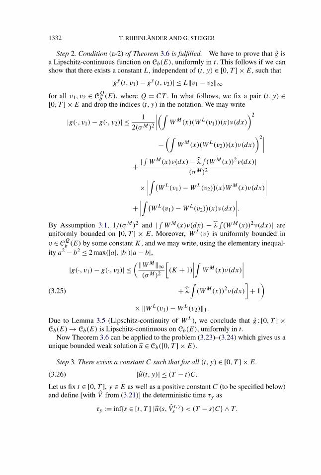
1332 T. RHEINLÄNDER AND G. STEIGER
Step 2. Condition (a-2) of Theorem 3.6 is fulfilled. We have to prove that g isa Lipschitz-continuous function on Cb(E), uniformly in t . This follows if we canshow that there exists a constant L, independent of (t, y) ∈ [0, T ] × E, such that
|gy(t, v1) − gy(t, v2)| ≤ L‖v1 − v2‖∞for all v1, v2 ∈ CQ
b (E), where Q = CT . In what follows, we fix a pair (t, y) ∈[0, T ] × E and drop the indices (t, y) in the notation. We may write
|g(·, v1) − g(·, v2)| ≤ 1
2(σM)2
∣∣∣∣(∫
WM(x)(WL(v1))(x)ν(dx)
)2
−(∫
WM(x)(WL(v2))(x)ν(dx)
)2∣∣∣∣+ | ∫ WM(x)ν(dx) − λ
∫(WM(x))2ν(dx)|
(σM)2
×∣∣∣∣∫ (
WL(v1) − WL(v2))(x)WM(x)ν(dx)
∣∣∣∣+
∣∣∣∣∫ (
WL(v1) − WL(v2))(x)ν(dx)
∣∣∣∣.By Assumption 3.1, 1/(σM)2 and | ∫ WM(x)ν(dx) − λ
∫(WM(x))2ν(dx)| are
uniformly bounded on [0, T ] × E. Moreover, WL(v) is uniformly bounded inv ∈ CQ
b (E) by some constant K , and we may write, using the elementary inequal-ity a2 − b2 ≤ 2 max(|a|, |b|)|a − b|,
|g(·, v1) − g(·, v2)| ≤(‖WM‖∞
(σM)2
[(K + 1)
∣∣∣∣∫
WM(x)ν(dx)
∣∣∣∣+ λ
∫(WM(x))2ν(dx)
]+ 1
)(3.25)
× ‖WL(v1) − WL(v2)‖1.
Due to Lemma 3.5 (Lipschitz-continuity of WL), we conclude that g : [0, T ] ×Cb(E) → Cb(E) is Lipschitz-continuous on Cb(E), uniformly in t .
Now Theorem 3.6 can be applied to the problem (3.23)–(3.24) which gives us aunique bounded weak solution u ∈ Cb([0, T ] × E).
Step 3. There exists a constant C such that for all (t, y) ∈ [0, T ] × E.
|u(t, y)| ≤ (T − t)C.(3.26)
Let us fix t ∈ [0, T ], y ∈ E as well as a positive constant C (to be specified below)and define [with V from (3.21)] the deterministic time τy as
τy := inf{s ∈ [t, T ] |u(s, V t,ys ) < (T − s)C} ∧ T .
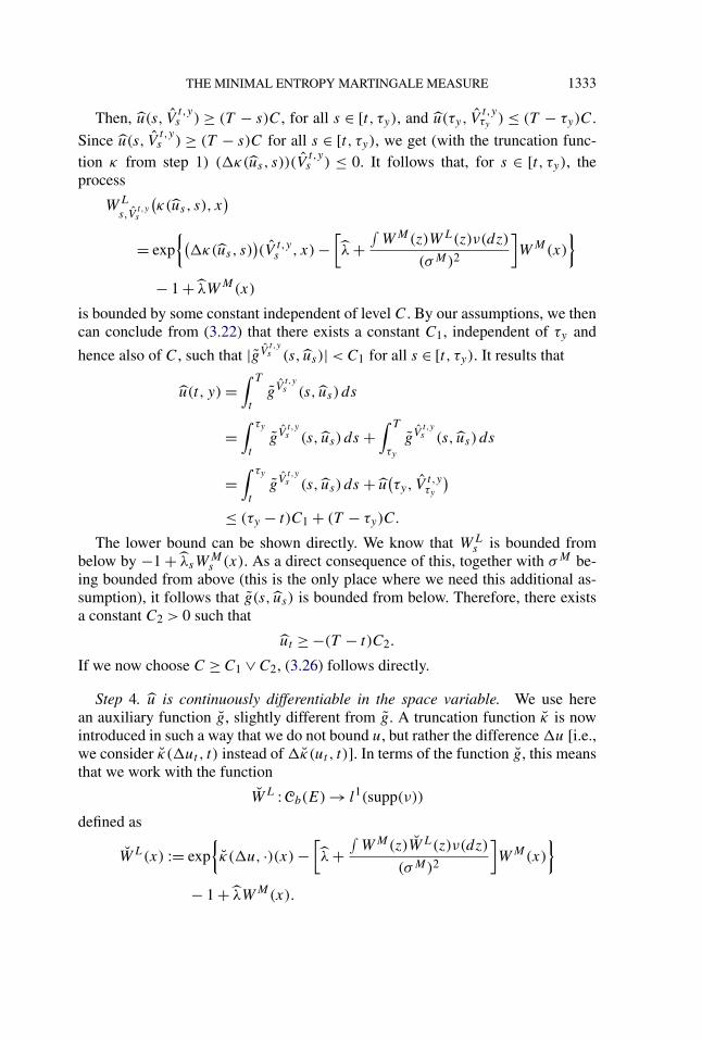
THE MINIMAL ENTROPY MARTINGALE MEASURE 1333
Then, u(s, Vt,ys ) ≥ (T − s)C, for all s ∈ [t, τy), and u(τy, V
t,yτy ) ≤ (T − τy)C.
Since u(s, Vt,ys ) ≥ (T − s)C for all s ∈ [t, τy), we get (with the truncation func-
tion κ from step 1) (�κ(us, s))(Vt,ys ) ≤ 0. It follows that, for s ∈ [t, τy), the
process
WL
s,Vt,ys
(κ(us, s), x
)
= exp{(
�κ(us, s))(V t,y
s , x) −[λ +
∫WM(z)WL(z)ν(dz)
(σM)2
]WM(x)
}
− 1 + λWM(x)
is bounded by some constant independent of level C. By our assumptions, we thencan conclude from (3.22) that there exists a constant C1, independent of τy and
hence also of C, such that |gVt,ys (s, us)| < C1 for all s ∈ [t, τy). It results that
u(t, y) =∫ T
tgV
t,ys (s, us) ds
=∫ τy
tgV
t,ys (s, us) ds +
∫ T
τy
gVt,ys (s, us) ds
=∫ τy
tgV
t,ys (s, us) ds + u
(τy, V
t,yτy
)≤ (τy − t)C1 + (T − τy)C.
The lower bound can be shown directly. We know that WLs is bounded from
below by −1 + λsWMs (x). As a direct consequence of this, together with σM be-
ing bounded from above (this is the only place where we need this additional as-sumption), it follows that g(s, us) is bounded from below. Therefore, there existsa constant C2 > 0 such that
ut ≥ −(T − t)C2.
If we now choose C ≥ C1 ∨ C2, (3.26) follows directly.
Step 4. u is continuously differentiable in the space variable. We use herean auxiliary function g, slightly different from g. A truncation function κ is nowintroduced in such a way that we do not bound u, but rather the difference �u [i.e.,we consider κ(�ut , t) instead of �κ(ut , t)]. In terms of the function g, this meansthat we work with the function
WL :Cb(E) → l1(supp(ν))
defined as
WL(x) := exp{κ(�u, ·)(x) −
[λ +
∫WM(z)WL(z)ν(dz)
(σM)2
]WM(x)
}
− 1 + λWM(x).

1334 T. RHEINLÄNDER AND G. STEIGER
In addition, to ensure that g(t, ut ) is differentiable, we assume that κ has the fol-lowing form, with w ∈ l∞(supp(ν)):
κ(w, t)(x) =
v(w), if |w(x)| ≤ (T − t)C,
ϕ(w, t)(x), if (T − t)C < |w(x)| < K + (T − t)C,
sign(w(x))(K + C(T − t)
),
if |w(x)| ≥ K + (T − t)C
for some fixed constants C, K and a suitable ϕ(w, t) ∈ l∞(supp(ν)) with|ϕ(w, t)(x)| ≤ K + (T − t)C, such that κ : l∞(supp(ν)) × [0, T ] → l∞(supp(ν))
is differentiable in w with uniformly bounded partial derivative.Reasoning as in Step 2, it follows that g is Lipschitz-continuous and, therefore,
we may apply Theorem 3.6, which provides a solution u. Let us consider u intro-duced above, which is bounded due to Step 3. That is, there exists a pair (C,K)
such that κ(�ut , t) = �ut and, therefore, g(t, ut ) = g(t, ut ). By uniqueness ofsolution, we conclude that u = u.
Let us now assume that ut ∈ C1b(E). By direct calculation,
∂
∂ygy(t, ut ) =
∫ (∂
∂yκ(�ut,y)(x)
)WL
t,y(x)ν(dx) + k(t, y, WL
t,y(�ut,y))
with WL(x) := WL(x) + 1 − λWM(x) and a uniformly bounded k(t, y,
WLt,y(�ut,y)). Let us now write
∂
∂ygy(t, ut ) =
∫∂
∂wκ(w, t)(x)
∣∣∣∣w=�ut,y
(∂
∂y�ut,y(x)
)WL
t,y(x)ν(dx)
+ k(t, y, WL
t,y(�ut,y))
=∫
∂
∂wκ(v, t)(x)
∣∣∣∣w=∫ WV
t,y (·)0 (∂/∂y)u(t,y+z) dz
×(
∂
∂yu(t, y + WV
t,y(x)) − ∂
∂yu(t, y)
)WL
t,y(x)ν(dx)
+ k
(t, y, WL
t,y
(∫ WVt,y(·)
0
∂
∂yu(t, y + z) dz
))
=: gy
(t,
∂
∂yut
).
Let us set vt (y) = ∂∂y
ut (y), which belongs to Cb(E). We already know that WL isuniformly continuous and bounded in (t, y, vt ) ∈ [0, T ] × E × Cb(E) and, there-fore, k is uniformly continuous and bounded on this set. On the other hand, takinginto account the definition of κ , it follows directly that condition (3.17) is fulfilledand that
∂
∂wκ(w, t)(x)
∣∣∣∣w=∫ WV
t,y (·)0 vt (y+z) dz

THE MINIMAL ENTROPY MARTINGALE MEASURE 1335
is uniformly continuous in (t, y, vt ) ∈ [0, T ] × E × M . Therefore, all conditionsof Theorem 3.7 are fulfilled and, hence, the solution u to the PDE (3.18) withboundary condition (3.19) is continuously differentiable in the space variable. �
Having proved the existence of a solution to the partial differential equa-tion (3.9) with boundary condition (3.10), we are in a position to determine thetriplet (φ,WL,σL) which solves equation (2.5). Since u is uniformly bounded, wedirectly see that this also holds for φ. The extra assumption that σM is boundedfrom above is not fulfilled in some examples. We shall indicate later, using theresult of Theorem 3.8, how to proceed in the standard BN–S model without thisassumption and still get a uniformly bounded φ.
THEOREM 3.9. Let Assumption 3.1 hold, and further assume that σM isuniformly bounded from above on [0, T ] × E. Let us assume that the triplet(φ,WL,σL) solves equation (2.5) as well as (2.3), with (φ,WL,σL) uniformlybounded. Then the process Z = (Zt ) defined by
Zt = dQ∗
dP
∣∣∣∣Ft
= E
(−
[∫(λσM −σL)dY c + (
λWM(x)−WL(x))∗ (µY − νY )
])t
is the density process of the MEMM.
PROOF. To show that Q∗ is the MEMM, we show that, according to ourapproach outlined in Remark 2.8, Q∗ is an equivalent martingale measure,
I (Q∗,P ) < ∞ and∫ φ
S− dS is a true Q-martingale for all Q ∈ Me with finiterelative entropy.
1. Q∗ is an equivalent martingale measure: Let us first show that it is an equiva-lent probability measure by checking the conditions of Lemma 2.11. We considerthe local martingale N defined by
N = −∫
λdM + L
(3.27)=
∫(σL − λσM)dY c + (
WL(x) − λWM(x)) ∗ (µY − νY ).
Since WL, λ and WM are bounded, N is locally bounded and due to
WL(x) − λWM(x) > −1,
we have �N > −1. Moreover, we set
U = 12
∫(σL − λσM)2 ds
+ {(1 − λWM(x) + WL(x)
)log
(1 − λWM(x) + WL(x)
)+ λWM(x) − WL(x)
} ∗ µY .

1336 T. RHEINLÄNDER AND G. STEIGER
Since λWM , WL ∈ l∞(supp(ν)) ∩ l1(supp(ν)) and λ, σM and σL are all uni-formly bounded, U has locally integrable variation and its compensator B is alsobounded. Hence, condition (2.7) is naturally fulfilled and, therefore, Q∗ is anequivalent probability measure. Finally, Q∗ is a martingale measure since its den-sity process can be written as
Z = E
(−
∫λdM + L
),
where L and [M,L] are locally bounded local P -martingales.2. I (Q∗,P ) < ∞: The density Z∗ = dQ∗
dPmay be written as
Z∗ = exp{c +
∫ T
0
φt
St−dSt
},
where c is the normalizing constant. We get
I (Q∗,P ) = EQ∗[c +
∫ T
0
φt
St−dSt
]
= EQ∗[c +
∫ T
0φt (η
Mt dt + σM
t dY ct ) + (
φWM(x) ∗ (µY − νY ))T
].
We must therefore show that
EQ∗[∫ T
0
φt
St−dSt
]= 0,(3.28)
since that implies I (Q∗,P ) = c, which is finite by the previous step. Introducing
νQ∗Y = (
1 − λWM(x) + WL(x)) ∗ νY ,(3.29)
it follows from Girsanov’s theorem that WM(x) ∗ (µY − νQ∗Y ) and
∫σM dY c +∫
(λσM − σL)σM dt are local Q∗-martingales. In fact, they are true Q∗-martinga-les since their quadratic variations are Q∗-integrable. This follows for the firstterm since 1 − λWM(x) + WL(x) is bounded, and WM is uniformly bounded andintegrable w.r.t. ν. For the second term, it follows from the boundedness of σM .Equation (3.28) follows since the dynamics of S can be written as
dSt
St−= σM
t dY ct + (λtσ
Mt − σL
t )σMt dt + d
(WM(x) ∗ (µY − ν
Q∗Y )
)t .
3.∫ φ
S− dS is a true Q-martingale for all Q ∈ Me with finite relative entropy. Inpreparation for this, let us observe that for any positive constant α we have
E[exp
{(α(WM(x))2 ∗ µY
)T
}]< ∞,(3.30)
E
[exp
{α
∫ T
0(σM
t )2 dt
}]< ∞.(3.31)

THE MINIMAL ENTROPY MARTINGALE MEASURE 1337
The first inequality follows from our assumption concerning WM since then
E[exp
{(α(WM(x))2 ∗ µY
)T
}] = exp{((
eα(WMt (x))2 − 1
) ∗ νY
)T
}< ∞
(see, e.g., [17], Lemma 14.39.1). Inequality (3.31) follows since σM is uniformlybounded.
We have that∫ φ
S− dS is a local Q-martingale. It will be a true Q-martingale byLemma 2.12 if we can show that, for some β > 0,
E
[exp
{β
∫ T
0
φ2t
S2t−
d[S]t}]
< ∞.
We denote k = supt∈[0,T ] ‖φ‖∞. Let us take β = 12k2 . By the Cauchy–Schwarz
inequality and (3.30), (3.31) we get
E
[exp
{β
∫ T
0
(φt
St−
)2
d[S]t}]
≤ E
[exp
{1
2
∫ T
0(σM
t )2 dt + 1
2
((WM(x))2 ∗ µY
)T
}]< ∞. �
4. Computing the MEMM in special cases.
4.1. The deterministic volatility case. The purpose of this section is to showhow we can recover some well-known results in our setup. We consider an assetprocess
dSt
St−= ηM(t,Vt ) dt + σM(t,Vt ) dY c
t + d(WM( · ,V−, x) ∗ (µY − νY )
)t ,
dVt = ηV (t,Vt ) dt,
fulfilling Assumptions 3.1.
COROLLARY 4.1. Let the bounded function φ : [0, T ] → R be such that(∣∣WM(x)(exp{φWM(x)} − 1
)∣∣ ∗ νY
)T < ∞,(4.1)
and that, for any t ∈ [0, T ], the following equation is fulfilled:
ηMt + (σM
t )2φt +∫
R
WMt (x)
(exp{φtW
Mt (x)} − 1
)νY (dx) = 0.(4.2)
Then, the MEMM Q∗ is given by
dQ∗
dP= exp
{c +
∫ T
0
φt
St−dSt
}

1338 T. RHEINLÄNDER AND G. STEIGER
(with normalizing constant c). Its density process can be written as
Zt = dQ∗
dP
∣∣∣∣Ft
= E
(∫φσM dY c + (
exp{φWM(x)} − 1) ∗ (µY − νY )
)t
.
PROOF. In the deterministic case we have �u = 0, since WV = 0. Hence, weobtain WL immediately from (3.3) as
WL(x) = λWM(x) − 1 + exp{φWM(x)}.Equation (4.2) then follows from equation (3.11) and the definition of λ. �
REMARK 4.2. Equation (4.2) corresponds to a condition well known in theliterature. For example, equation (3.20) in [7], condition (C) in [14], condition (4.4)in Theorem B in [11], or equation (4.30) in Theorem 4.3 of [8]. For more referencescontaining this condition (or an equivalent form of it) we refer to [11].
4.2. The orthogonal volatility case. Let us consider the asset process
dSt
St−= ηM(t,Vt ) dt + σM(t,Vt ) dY c
t ,
dVt = ηV (t,Vt ) dt + d(WV (·,V−, x) ∗ µY
)t ,
fulfilling Assumptions 3.1 so that, in particular,
λ = ηM
(σM)2
is bounded. Assume that E is compact so that σM is bounded as well. We then getthe following result:
COROLLARY 4.3. The optimal strategy is
φ = −λ,(4.3)
and the density process of the MEMM is given via
WL(t,Vt−, x) = v(t,Vt− + WVt (x))
v(t,Vt−)− 1,
σL(t,Vt−) = 0,
where v is the classical solution of the partial differential equation
∂
∂tv(t, y) + ηV
t
∂
∂yv(t, y) − 1
2λ2
t (σMt )2v(t, y)
(4.4)+
∫R
(v(t, y + WV
t (x)) − v(t, y)
)ν(dx) = 0,
v(T , y) = 1.(4.5)

THE MINIMAL ENTROPY MARTINGALE MEASURE 1339
PROOF. Equation (4.3) and σL = 0 are direct consequences of WM(x) = 0and equation (3.11). Further, (3.12) leads to
WL(t,Vt−, x) = exp{u(t, Vt− + WV
t (x)) − u(t,Vt−)
} − 1.(4.6)
We know from Theorem 3.8 that∂
∂tu(t, y) + ηV
t
∂
∂yu(t, y) − 1
2λ2
t (σMt )2 +
∫WL(t, y, x)ν(dx) = 0,
(4.7)u(T , y) = 0
has a classical bounded solution u, from which we can determine (φ,WL,σL) andhence the MEMM by Theorem 3.9. Using the transformation v(t, y) = expu(t, y),we get the linear boundary problem (4.4), (4.5). �
REMARK 4.4. 1. The optimal strategy in this specific case had already beenidentified by Grandits and Rheinländer [16] by a conditioning argument. How-ever, while the density of the MEMM at a fixed time T has a very simple form,the corresponding density process turns out to have a more complicated structure.Becherer [2] determines the density process in a model where the volatility processswitches between a finite number of states.
2. The transformation v(t, y) = expu(t, y) is very useful here since it linearizesthe partial differential equation to (4.4). However, this does not apply to the gen-eral case when the jump process directly influences the asset process. As can beseen already in the deterministic volatility case, the exponential element cannot belinearized in this way.
3. Benth and Meyer-Brandis [6] determined the MEMM for the specific case ofa simplified BN–S model where no jumps occur in the price process, but with σM
possibly unbounded. We need the boundedness of σM only if we refer to Theo-rem 3.8 for the existence of the IPDE (4.7). Alternatively, one could directly appealto an existence result for the linear IPDE (4.4) and then carry out the relevant ver-ification steps, imposing analogous conditions as in [6].
4. It follows from (3.29) that the measure νQY , where Q is the MEMM, is given
by νQY = (WL(x) + 1) ∗ νY . Since WL is specified by (4.6), in general it is a non-
deterministic process and, in that case, Y cannot be an additive process under Q.We conclude that the MEMM is not in general contained in the class of structure-preserving martingale measures as considered in [24].
4.3. The Barndorff-Nielsen Shephard model with jumps. In [1] the priceprocess of a stock S = (St )t∈[0,T ] is defined by the exponential exp{Xt } withX = (Xt) satisfying
dXt = (µ + βσ 2t ) dt + σt dY c
t + d(ρx ∗ µY )t ,
dσ 2t = −λσ 2
t dt + d(x ∗ µY )t ,
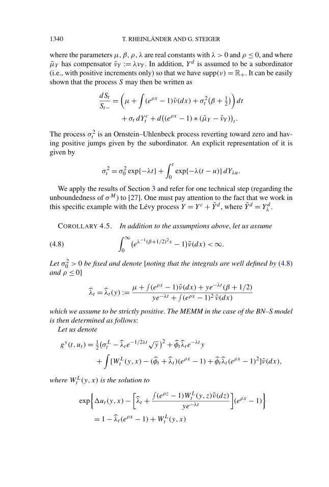
1340 T. RHEINLÄNDER AND G. STEIGER
where the parameters µ,β,ρ,λ are real constants with λ > 0 and ρ ≤ 0, and whereµY has compensator νY := λνY . In addition, Yd is assumed to be a subordinator(i.e., with positive increments only) so that we have supp(ν) = R+. It can be easilyshown that the process S may then be written as
dSt
St−=
(µ +
∫(eρx − 1)ν(dx) + σ 2
t
(β + 1
2
))dt
+ σt dY ct + d
((eρx − 1) ∗ (µY − νY )
)t .
The process σ 2t is an Ornstein–Uhlenbeck process reverting toward zero and hav-
ing positive jumps given by the subordinator. An explicit representation of it isgiven by
σ 2t = σ 2
0 exp{−λt} +∫ t
0exp{−λ(t − u)}dYλu.
We apply the results of Section 3 and refer for one technical step (regarding theunboundedness of σM ) to [27]. One must pay attention to the fact that we work inthis specific example with the Lévy process Y = Y c + Y d , where Y d = Yd
λ .
COROLLARY 4.5. In addition to the assumptions above, let us assume∫ ∞0
(eλ−1(β+1/2)2x − 1
)ν(dx) < ∞.(4.8)
Let σ 20 > 0 be fixed and denote [noting that the integrals are well defined by (4.8)
and ρ ≤ 0]
λt = λt (y) := µ + ∫(eρx − 1)ν(dx) + ye−λt (β + 1/2)
ye−λt + ∫(eρx − 1)2 ν(dx)
which we assume to be strictly positive. The MEMM in the case of the BN–S modelis then determined as follows:
Let us denote
gy(t, ut ) = 12
(σL
t − λt e−1/2λt√y
)2 + φt λt e−λty
+∫
[WLt (y, x) − (φt + λt )(e
ρx − 1) + φt λt (eρx − 1)2]ν(dx),
where WLt (y, x) is the solution to
exp{�ut(y, x) −
[λt +
∫(eρz − 1)WL
t (y, z)ν(dz)
ye−λt
](eρx − 1)
}
= 1 − λt (eρx − 1) + WL
t (y, x)

THE MINIMAL ENTROPY MARTINGALE MEASURE 1341
and
�ut(y, x) = u(t, y + eλtx) − u(t, y),
φt = −∫(eρx − 1)WL
t (y, x)ν(dx)
ye−λt− λt ,
σLt = −
∫(eρx − 1)WL
t (y, x)ν(dx)√ye−(1/2)λt
.
Then, the classical solution u of the integro-PDE
∂
∂tu(t, y) + gy(t, ut ) = 0,(4.9)
u(T , y) = 0 ∀y ∈ E := [σ 20 ,∞)(4.10)
determines the MEMM via WL and σL:
Zt = dQ∗
dP
∣∣∣∣Ft
= E
(∫(−λsσs + σL
s ) dY cs + (−λ(eρx − 1) + WL(x)
) ∗ (µY − νY )
)t
.
As σ is in general not bounded, we may not directly apply Theorem 3.8 to provethat there exists a classical solution u to the problem (4.9)–(4.10). Resolving thisissue has turned out to be surprisingly technical and has been carried out in [27],Chapter 6.6. The existence of a solution is there constructed via an Arzela–Ascoliargument from solutions which live on compact sets (their existence is thereforeguaranteed by Theorem 3.8). Let us summarize this analysis:
THEOREM 4.6 ([27]). Under the assumptions of Corollary 4.5, there exists aclassical solution u of the integro-PDE (4.9), (4.10) such that �u is bounded fromabove on [0, T ] × E.
PROOF OF COROLLARY 4.5. The IPDE (4.9) with boundary condition (4.10)can be derived from the results in Section 3 by making the transformation
σ 2t = eλtσ 2
t
such that we obtain the dynamics
dSt
St−=
(µ + λ
∫(eρx − 1)ν(dx) + e−λt σ 2
t
(β + 1
2
))dt
+ e−(1/2)λt σt dY ct + d
((eρx − 1) ∗ (µY − νY )
)t
with
dσ 2t = d(eλ·x ∗ µY )t .

1342 T. RHEINLÄNDER AND G. STEIGER
By Theorem 4.6, we have a classical solution u, with �u bounded from above, soit follows from Lemma 3.3.1 that WL is uniformly bounded and integrable w.r.t. ν.
Based on this result, we now show that the three conditions of Remark 2.8 arefulfilled:
1. Q∗ is an equivalent martingale measure: here we proceed similarly as inthe proof of Theorem 3.9 and concentrate only on verifying the conditions ofLemma 2.11. Let us consider
U = 12
∫φ2σ 2 ds + WU(x) ∗ µY
with
WU(x) := (WL(x) + 1 − λ(eρx − 1)
)log
(WL(x) + 1 − λ(eρx − 1)
)+ λ(eρx − 1) − WL(x).
Since eρx −1 and WL are uniformly bounded and integrable w.r.t. ν, U has locallyintegrable variation, and we get
E[exp
{2λ
(WU(x) ∗ ν
)T
}]< ∞.
Hence (2.7) is fulfilled by the Cauchy–Schwarz inequality if we can show that
E
[exp
{∫ T
0φ2
t σ2t dt
}]< ∞.
By definition, we have
φt = −λt −∫(eρx − 1)WL
t (x)ν(dx)
σ 2t−
.
Since λ is positive and WL is bounded, φt is negative for sufficiently large σt−.Let us introduce σ such that for all t ∈ [0, T ] (with the possible exception of aLebesgue-zero set)
φt < 0 for all σt > σ .
On the other hand, since WLt (x) ≥ −1 + λt (e
ρx − 1), φt is bounded from belowwith
φt ≥ −λt −∫(eρx − 1)(−1 + λt (e
ρx − 1))ν(dx)
σ 2t−
= −(β + 1
2
)− µ
σ 2t−
because of
λt = µ + ∫(eρx − 1)ν(dx) + σ 2
t−(β + 1/2)
σ 2t− + ∫
(eρx − 1)2ν(dx).

THE MINIMAL ENTROPY MARTINGALE MEASURE 1343
Let us now analyze
E
[exp
{∫ T
0φ2
t σ2t dt
}]
= E
[exp
{∫ T
01{σt≤σ }φ2
t σ2t dt
}exp
{∫ T
01{σt>σ }φ2
t σ2t dt
}].
We have that
exp{∫ T
01{σt≤σ }φ2
t σ2t dt
}
is uniformly bounded. Moreover,
E
[exp
{∫ T
01{σt>σ }φ2
t σ2t dt
}]
is finite due to (i) the fact that for almost all t
0 ≥ φt ≥ −(β + 1
2
)− µ
σ 2t
on the set {σt > σ } and (ii) condition (4.8), which, according to Benth, Karlsenand Reikvam ([5], Lemma 3.1), ensures that
E
[exp
{(β + 1
2
)2∫ T
0σ 2
t dt
}]< ∞.
2. I (Q∗,P ) < ∞: We have to show that for νQ∗Y = (WL(x) + 1 − λ(eρx −
1)) ∗ νY ,
(eρx − 1) ∗ (µY − νQ∗Y ) and
∫σ dY c +
∫(λσ − σL)σ dt
are true Q∗-martingales, that is, their quadratic variations are Q∗-integrable. Thisfollows for the first term from the boundedness of WL and the integrability ofeρx − 1. For the second term, let us consider
EQ∗[[∫
σ dY c
]T
]= EQ∗
[∫ T
0σ 2
t dt
].
It is well known that we may write∫ T
0σ 2
t dt = λ−1(1 − e−λT )σ 20 + (
λ−1(1 − e−λ(T −·))x ∗ µY
)T .
Hence, EQ∗[∫ T0 σ 2
t dt] is finite if EQ∗[(x ∗ νQ∗Y )T ] is finite, which, since WL is
bounded, is equivalent to showing that∫
xν(dx) < ∞. However, this follows fromcondition (4.8).
1344 T. RHEINLÄNDER AND G. STEIGER
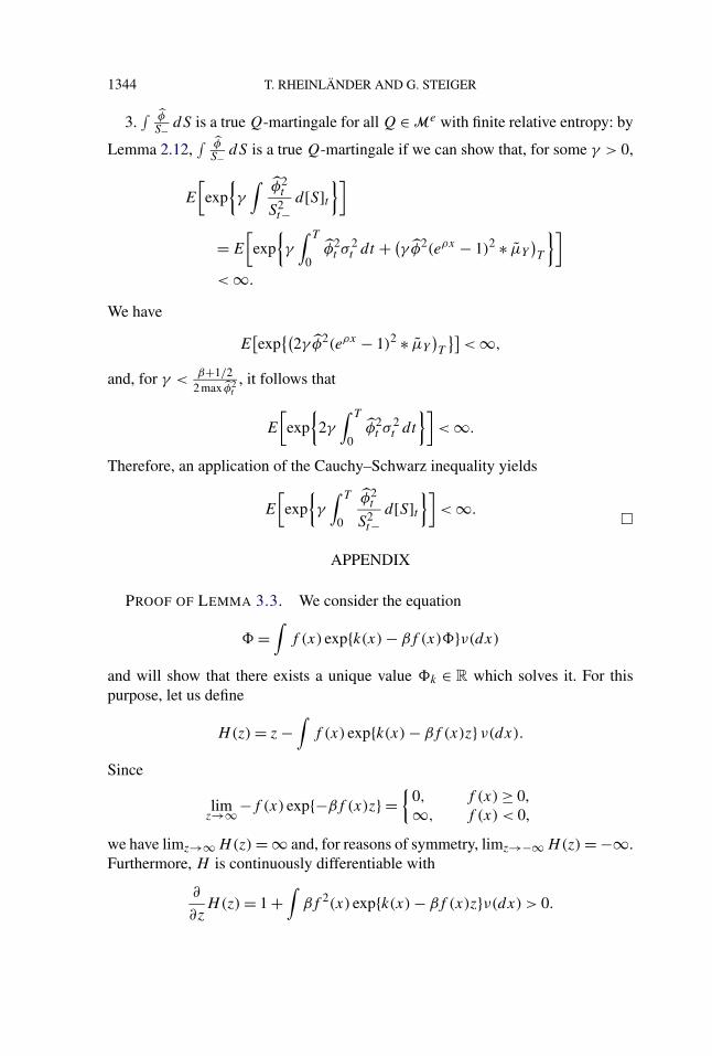
3.∫ φ
S− dS is a true Q-martingale for all Q ∈ Me with finite relative entropy: by
Lemma 2.12,∫ φ
S− dS is a true Q-martingale if we can show that, for some γ > 0,
E
[exp
{γ
∫φ2
t
S2t−
d[S]t}]
= E
[exp
{γ
∫ T
0φ2
t σ2t dt + (
γ φ2(eρx − 1)2 ∗ µY
)T
}]< ∞.
We have
E[exp
{(2γ φ2(eρx − 1)2 ∗ µY
)T
}]< ∞,
and, for γ <β+1/2
2 max φ2t
, it follows that
E
[exp
{2γ
∫ T
0φ2
t σ2t dt
}]< ∞.
Therefore, an application of the Cauchy–Schwarz inequality yields
E
[exp
{γ
∫ T
0
φ2t
S2t−
d[S]t}]
< ∞. �
APPENDIX
PROOF OF LEMMA 3.3. We consider the equation
� =∫
f (x) exp{k(x) − βf (x)�}ν(dx)
and will show that there exists a unique value �k ∈ R which solves it. For thispurpose, let us define
H(z) = z −∫
f (x) exp{k(x) − βf (x)z}ν(dx).
Since
limz→∞−f (x) exp{−βf (x)z} =
{0, f (x) ≥ 0,∞, f (x) < 0,
we have limz→∞ H(z) = ∞ and, for reasons of symmetry, limz→−∞ H(z) = −∞.Furthermore, H is continuously differentiable with
∂
∂zH(z) = 1 +
∫βf 2(x) exp{k(x) − βf (x)z}ν(dx) > 0.

THE MINIMAL ENTROPY MARTINGALE MEASURE 1345
Therefore, there exists a unique �k ∈ R such that H(�k) = 0. We can moreovershow that
|�k| ≤ maxx∈supp(ν)
{exp k(x)}∫
|f (x)|ν(dx).
Let us assume that �k ≥ 0. Then, we get
�k =∫
f (x) exp{k(x) − βf (x)�k}ν(dx)
≤∫{f (x)>0}
f (x) exp{k(x) − βf (x)�k}ν(dx)
≤∫{f (x)>0}
f (x) exp{k(x)}ν(dx)
≤ maxx∈supp(ν)
{expk(x)}∫{f (x)>0}
f (x)ν(dx)
≤ maxx∈supp(ν)
{expk(x)}∫
|f (x)|ν(dx).
The lower bound can be shown in exactly the same way.Let us now define the bounded function
ϕk(x) := exp{k(x) − βf (x)�k}.As we have∫
f (x)ϕk(x)ν(dx) =∫
f (x) exp{k(x) − βf (x)�k}ν(dx) = �k,
it follows that
ϕk(x) = exp{k(x) − βf (x)
∫f (z)ϕk(z)ν(dz)
},
and, therefore, we conclude that ϕ := ϕk is well defined and bounded. �
PROOF OF LEMMA 3.5. Since WL is bounded on CQb (E), we only have to
show local Lipschitz-continuity of WL, that is, we have to show that for any c > 0,there exists a constant Lc such that
‖WL(v1) − WL(v2)‖1 ≤ Lc‖v1 − v2‖∞for all v1, v2 ∈ CQ
b (E) with ‖v1 − v2‖∞ ≤ c2 . For that purpose, consider v0 + rh,
where v0 ∈ CQb (E) and h ∈ CQ
b (E) with ‖h‖∞ = c2 , and r ∈ [0,1].
Let k be bounded from above and define
ϕk(x) := exp{k(x) − WM(x)
(σM)2
∫WM(z)ϕk(z)ν(dz)
},
�k :=∫
WM(x)ϕk(x)ν(dx).

1346 T. RHEINLÄNDER AND G. STEIGER
By equation (3.12), we may write
ϕk∗(r) = WL(v0 + rh) − λWM + 1
for
k∗(r) = �v0 + r�h − WM η
and
η := λ
(1 +
∫(WM(z))2ν(dz)
(σM)2
)−
∫WM(z)ν(dz)
(σM)2 .
The goal is to show that there is a constant C1 such that, for all r ∈ [0,1],∥∥ϕk∗(r) − ϕk∗(0)
∥∥1 ≤ C1‖rh‖∞ = C1rc
2.(A.1)
Let us therefore analyze∣∣(ϕk∗(r) − ϕk∗(0)
)(x)
∣∣= exp{�v0(x) − ηWM(x)}
×∣∣∣∣exp
{r�h(x) − �k∗(r)
WM(x)
(σM)2
}− exp
{−�k∗(0)
WM(x)
(σM)2
}∣∣∣∣(A.2)
= exp{�v0(x) − ηWM(x) − �k∗(0)
WM(x)
(σM)2
}
×∣∣∣∣exp
{r�h(x) − (
�k∗(r) − �k∗(0)
)WM(x)
(σM)2
}− 1
∣∣∣∣.Since v0 is uniformly bounded by Q, the first term on the right-hand side is uni-formly bounded for all x ∈ supp(ν). The second term [to be labeled fx(r)] needsfurther investigation. For this purpose, let us state the following property of �k :
CLAIM 1. Given two functions k1, k2 ∈ l∞(supp(ν)) with{k1(x) ≤ k2(x) ∀x ∈ supp(ν) s.t. WM(x) < 0,k1(x) ≥ k2(x) ∀x ∈ supp(ν) s.t. WM(x) > 0,
it follows that �k1 ≥ �k2 .
PROOF. Let us assume that �k1 < �k2 . For any x ∈ supp(ν), it then followsthat
ϕk2(x)
ϕk1(x)= exp
{k2(x) − k1(x) − WM(x)
(σM)2
(�k2 − �k1
)}{
> 1, ∀x ∈ supp(ν) s.t. WM(x) < 0,< 1, ∀x ∈ supp(ν) s.t. WM(x) > 0.

THE MINIMAL ENTROPY MARTINGALE MEASURE 1347
However, this leads to a contradiction, since then
�k2 − �k1 =∫
WM(x)(ϕk2(x) − ϕk1(x)
)ν(dx) ≥ 0.
Therefore, we must have �k1 ≥ �k2 . �
Let us now fix x0 ∈ supp(ν) and analyze the term
fx0(r) := exp{r�h(x0) − (
�k∗(r) − �k∗(0)
)WM(x0)
(σM)2
}− 1.
Obviously, we have fx0(0) = 0. Let us now assess the upper and lower boundsof fx0 for r ∈ [0,1]. For this purpose, we introduce
k+(r, x) := �v0(x) − WM(x)η + rc(1{WM(x)>0} − 1{WM(x)<0}
)(x),
k−(r, x) := �v0(x) − WM(x)η − rc(1{WM(x)>0} − 1{WM(x)<0}
)(x).
We will use in the following the notation
1∗(x) := 1{WM(x)>0} − 1{WM(x)<0}.It follows from the claim above that
�k−(r) − �k−(0) ≤ �k∗(r) − �k∗(0) ≤ �k+(r) − �k+(0).(A.3)
Let us now consider in detail the upper bound,
�k+(r) − �k+(0) =∫ r
0
∂
∂r�k+(s) ds.
Here the existence of the derivative can be guaranteed by an application of theImplicit Function Theorem for Banach spaces (see, e.g., [28], page 150) to theequation
�k+(r) =∫
WM(x) exp{k+(r, x) − WM(x)
(σM)2 �k+(r)
}ν(dx).
We have
∂
∂r�k+(r) =
∫WM(x)
[c1∗(x) − WM(x)
(σM)2
∂
∂r�k+(r)
]
× exp{k+(r, x) − WM(x)
(σM)2 �k+(r)
}ν(dx),
so we may write [recalling that ϕk+(r)(x) = exp{k+(r, x) − WM(x)
(σM)2 �k+(r)}]∂
∂r�k+(r) = c
( ∫WM(x)1∗(x)ϕk+(r)(x)ν(dx)
1 + ∫((WM(x))2/(σM)2)ϕk+(r)(x)ν(dx)
)
< c
∫|WM(x)|ϕk+(r)(x)ν(dx).

1348 T. RHEINLÄNDER AND G. STEIGER
Since k+(s) is bounded from above, it follows from the definition of ϕk+(s)
and Lemma 3.3 that ϕk+(s) is uniformly bounded by some constant K∗ for anys ∈ [0, r]. Therefore, it follows that
�k+(r) − �k+(0) < crK∗∫
|WM(x)|ν(dx).
Applying the same steps to the lower bound, it follows that
�k−(r) − �k−(0) > −crK∗∫
|WM(x)|ν(dx).
Taking into account the inequalities of (A.3), we obtain the following bounds:
exp{rcK(x0)} − 1 ≥ fx0(r) ≥ exp{−rcK(x0)} − 1
with
K(x0) := 1 + K∗ |WM(x0)|(σM)2
∫|WM(x)|ν(dx).
Therefore, for r ∈ [0,1], it follows that
|fx(r)| ≤ rcK(x)
with K ∈ l1(supp(ν)), and hence, via (A.1), the Lipschitz-continuity of WL isshown. �
PROOF OF THEOREM 3.6. Let us fix some u ∈ Cb([0, T ] × E) and considerthe PDE
∂
∂tw(t, z) + b(t, z)
∂
∂zw(t, z) + gz(t, ut ) = 0,(A.4)
w(T , z) = h(z) ∀ z ∈ E.(A.5)
It is straightforward to see that
w(t, z) = h(Zt,zT ) +
∫ T
tgZ
t,zs (s, us) ds
solves the boundary problem in the weak sense. Let us introduce the operatorF :Cb([0, T ] × E) → Cb([0, T ] × E) defined as follows:
(Fu)(t, z) = h(Zt,zT ) +
∫ T
tgZ
t,zs (s, us) ds.
We have to prove that F is a contraction on the space Cb([0, T ] × E). Let us,for some β ∈ R+, consider the norm
‖u‖β := sup(t,z)∈[0,T ]×E
e−β(T −t)|u(t, z)|,

THE MINIMAL ENTROPY MARTINGALE MEASURE 1349
which is equivalent to the supremum-norm ‖u‖∞. Due to condition (a-2), we ob-tain for u1, u2 ∈ Cb([0, T ] × E)
e−β(T −t)|(Fu1)(t, z) − (Fu2)(t, z)|= 1
eβ(T −t)
∣∣∣∣∫ T
t
(gZ
t,zs (s, u1,s) − gZ
t,zs (s, u2,s)
)ds
∣∣∣∣≤ 1
eβ(T −t)
∫ T
t
∣∣gZt,zs (s, u1,s) − gZ
t,zs (s, u2,s)
∣∣e−β(T −s)eβ(T −s) ds
≤ 1
eβ(T −t)L‖u1 − u2‖β
∫ T
teβ(T −s) ds
≤ L
β‖u1 − u2‖β
for all t ∈ [0, T ] and z ∈ E. Thus,
‖(Fu1)(t, z) − (Fu2)(t, z)‖β ≤ L
β‖u1 − u2‖β,
and F is a contraction on the normed space (Cb([0, T ] × E),‖ · ‖β) with β > L.Therefore, there exists a unique fixed point u ∈ Cb([0, T ] × E) which satisfies thePDE (3.15)–(3.16) in the weak sense. �
PROOF OF THEOREM 3.7. Let us analyze the operator G :Cb([0, T ] × E) →Cb([0, T ] × E), defined by
(Gv)(t, z) = ∂
∂zh(Z
t,zT ) +
∫ T
t
(∂
∂zZt,z
s
)gZ
t,zs (s, vs) ds.
Let us first discuss ∂∂z
Zt,zs , which is well defined by Protter [25], Theorem V.39.
Differentiating (3.14), we get
∂
∂zZt,z
s = 1 +∫ s
t
(∂
∂zZt,z
u
)∂
∂Zt,zu
b(u,Zt,zu ) du.
By Gronwall’s lemma, we can directly conclude that ∂∂z
Zt,zs is uniformly bounded,
the bound being denoted by LZ . Analogously, let us denote Lh := ‖h′‖∞.Let us now discuss, for v ∈ Cb([0, T ] × E),
e−β(T −t)|(Gv)(t, z)|≤ e−β(T −t)
(∣∣∣∣ ∂
∂zZt,z
s
∣∣∣∣|h′(Zt,zT )| +
∫ T
t
∣∣∣∣ ∂
∂zZt,z
s
∣∣∣∣∣∣gZt,zs (s, vs)
∣∣ds
)
≤ e−β(T −t)LZ
(Lh +
∫ T
t(L‖vs‖∞ + K)e−β(T −t)eβ(T −t) ds
)
≤ LZL
β‖v‖β + LZKT + LZLh.
1350 T. RHEINLÄNDER AND G. STEIGER
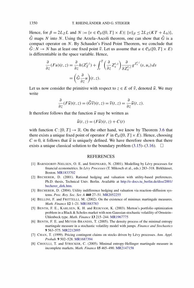
Hence, for β = 2LZL and N := {v ∈ Cb([0, T ] × E)| ‖v‖β ≤ 2LZ(KT + Lh)},G maps N into N . Using the Arzela–Ascoli theorem, one can show that G is acompact operator on N . By Schauder’s Fixed Point Theorem, we conclude thatG :N → N has at least one fixed point v. Let us assume that u ∈ Cb([0, T ] × E)
is differentiable in the space variable. Hence,
∂
∂z(Fu)(t, z) = ∂
∂zh(Z
t,zT ) +
∫ T
t
(∂
∂zZt,z
s
)∂
∂Zt,zs
gZt,zs (s, us) ds
=(G
∂
∂zu
)(t, z).
Let us now consider the primitive with respect to z ∈ E of v, denoted u. We maywrite
∂
∂z(F u)(t, z) = (Gv)(t, z) = v(t, z) = ∂
∂zu(t, z).
It therefore follows that the function u may be written as
u(t, z) = (F u)(t, z) + C(t)
with function C : [0, T ] → R. On the other hand, we know by Theorem 3.6 thatthere exists a unique fixed point of operator F in Cb([0, T ]×E). Hence, choosingC ≡ 0, it follows that u is uniquely defined. We have therefore shown that thereexists a unique classical solution to the boundary problem (3.15)–(3.16). �
REFERENCES
[1] BARNDORFF-NIELSEN, O. E. and SHEPHARD, N. (2001). Modelling by Lévy processes forfinancial econometrics. In Lévy Processes (T. Mikosch et al., eds.) 283–318. Birkhäuser,Boston. MR1833702
[2] BECHERER, D. (2001). Rational hedging and valuation with utility-based preferences.Ph.D. thesis, Technical Univ. Berlin. Available at http://e-docs.tu_berlin.de/diss/2001/becherer_dirk.htm.
[3] BECHERER, D. (2004). Utility indifference hedging and valuation via reaction–diffusion sys-tems. Proc. Roy. Soc. Ser. A 460 27–51. MR2052255
[4] BELLINI, F. and FRITTELLI, M. (2002). On the existence of minimax martingale measures.Math. Finance 12 1–21. MR1883783
[5] BENTH, F. E., KARLSEN, K. H. and REIKVAM, K. (2003). Merton’s portfolio optimizationproblem in a Black & Scholes market with non-Gaussian stochastic volatility of Ornstein–Uhlenbeck type. Math. Finance 13 215–244. MR1967775
[6] BENTH, F. E. and MEYER-BRANDIS, T. (2005). The density process of the minimal entropymartingale measure in a stochastic volatility model with jumps. Finance and Stochastics9 563–575. MR2212895
[7] CHAN, T. (1999). Pricing contingent claims on stocks driven by Lévy processes. Ann. Appl.Probab. 9 502–528. MR1687394
[8] CHOULLI, T. and STRICKER, C. (2005). Minimal entropy-Hellinger martingale measure inincomplete markets. Math. Finance 15 465–490. MR2147158

THE MINIMAL ENTROPY MARTINGALE MEASURE 1351
[9] DELBAEN, F., GRANDITS, P., RHEINLÄNDER, T., SAMPERI, D., SCHWEIZER, M. andSTRICKER, CH. (2002). Exponential hedging and entropic penalties. Math. Finance 1299–123. MR1891730
[10] DELLACHERIE, C. and MEYER, P.-A. (1980). Probabilités et Potentiel, 2nd ed. Hermann,Paris. MR0566768
[11] ESCHE, F. and SCHWEIZER, M. (2005). Minimal entropy preserves the Lévy property: Howand why. Stochastic Process. Appl. 115 299–327. MR2111196
[12] FÖLLMER, H. and SCHWEIZER, M. (1991). Hedging of contingent claims under incompleteinformation. In Applied Stochastics Monographs (M. H. A. Davis and R. J. Elliott, eds.)5 389–414. Gordon and Breach, New York. MR1108430
[13] FRITTELLI, M. (2000). The minimal entropy martingale measure and the valuation problem inincomplete markets. Math. Finance 10 39–52. MR1743972
[14] FUJIWARA, T. and MIYAHARA, Y. (2003). The minimal entropy martingale measures for geo-metric Lévy processes. Finance and Stochastics 7 509–531. MR2014248
[15] GRANDITS, P. (1999). On martingale measures for stochastic processes with independent in-crements. Theory Probab. Appl. 44 39–50. MR1751190
[16] GRANDITS, P. and RHEINLÄNDER, T. (2002). On the minimal entropy martingale measure.Ann. Probab. 30 1003–1038. MR1920099
[17] HE, S., WANG, J. and YAN, J. (1992). Semimartingale Theory and Stochastic Calculus. Sci-ence Press and CRC Press, Beijing. MR1219534
[18] HOBSON, D. (2004). Stochastic volatility models, correlation and the q-optimal measure.Math. Finance 14 537–556. MR2092922
[19] JACOD, J. and SHIRYAEV, A. (2003). Limit Theorems for Stochastic Processes, 2nd ed.Springer, Berlin. MR1943877
[20] KALLSEN, J. (2001). Utility-based derivative pricing in incomplete markets. In MathematicalFinance—Bachelier Congress 2000 (H. Geman et al., eds.) 313–338. Springer, Berlin.MR1960570
[21] LEPINGLE, D. and MÉMIN, J. (1978). Sur l’intégrabilité uniforme des martingales exponen-tielles. Z. Wahrsch. Verw. Gebiete 42 175–203. MR0489492
[22] MANDELBROT, B. (1963). The variation of certain speculative prices. J. Business 36 392–417.[23] MIYAHARA, Y. (2001). Geometric Lévy Processes and MEMM pricing model and related
estimation problems. Financial Engineering and the Japanese Markets 8 45–60.[24] NICOLATO, E. and VENARDOS, E. (2003). Option pricing in stochastic volatility models of
the Ornstein–Uhlenbeck type. Math. Finance 13 445–466. MR2003131[25] PROTTER, P. (2004). Stochastic Integration and Differential Equations—A New Approach,
2nd ed. Springer, Berlin. MR1037262[26] RHEINLÄNDER, T. (2005). An entropy approach to the Stein and Stein model with correlation.
Finance and Stochastics 9 399–413. MR2211715[27] STEIGER, G. (2005). The optimal martingale measure for investors with exponential utility
function. Ph.D. thesis, ETH Zürich. Available http://www.math.ethz.ch/~gsteiger.[28] ZEIDLER, E. (1986). Nonlinear Functional Analysis and its Applications I. Fixed-Point Theo-
rems. Springer, New York. MR0816732
DEPARTMENT OF STATISTICS
LONDON SCHOOL OF ECONOMICS
LONDON WC2A 2AEUNITED KINGDOM
E-MAIL: [email protected]
D-MATH, ETH-ZENTRUM
ETH ZÜRICH
CH-8092 ZÜRICH
SWITZERLAND
E-MAIL: [email protected]