RESEARCH ARTICLE Open Access

Three-dimensional protein model similarityanalysis based on salient shape indexBo Yao, Zhong Li*, Meng Ding and Minhong Chen

Abstract

Background: Proteins play a special role in bioinformatics. The surface shape of a protein, which is an importantcharacteristic of the protein, defines a geometric and biochemical domain where the protein interacts with otherproteins. The similarity analysis among protein models has become an important topic of protein analysis, by whichit can reveal the structure and the function of proteins.

Results: In this paper, a new protein similarity analysis method based on three-dimensional protein models isproposed. It constructs a feature matrix descriptor for each protein model combined by calculating the shape index(SI) and the related salient geometric feature (SGF), and then analyzes the protein model similarity by using thisfeature matrix and the extended grey relation analysis.

Conclusions: We compare our method to the Multi-resolution Reeb Graph (MRG) skeleton method, the L1-medialskeleton method and the local-diameter descriptor method. Experimental results show that our protein similarityanalysis method is accurate and reliable while keeping the high computational efficiency.

Keywords: Protein model, Shape index, Salient geometric feature, Shape analysis

BackgroundProtein similarity analysis is an important topic in bio-informatics. With it, we can help understand the structureand the function of proteins. The protein shape analysisplays an important role in medical research, computeraided molecular design, protein structure retrieval andprediction, among others. However, the analysis is highlychallenging due to the complexity of a protein’s three-dimensional surface shape, which can deform significantlyenough to change the topological structure during mo-lecular interactions [1].Many researchers have contributed to similarity ana-

lysis methods for comparing protein shapes. Via et al.[2] gave a survey on the current knowledge of the pro-tein surface similarity. The similarity analysis methodbased on comparison of shape feature is a common ap-proach. Sael et al. [3] proposed a popular protein surfacesimilarity method based on a 3D Zernike descriptor.Compactness and rotational invariance of this descriptorenable fast comparison suitable for protein databasesearches. However, in order to capture the high resolution

of the protein surface similarity, computation increases asthe number of terms in its series expansion increases. Andit is not applicable for the protein models with complextopology such as holes. Osada et al. [4] provided a shapedistribution method based on the statistical histogram thatmeasures the vertex distribution of the whole model sur-face, from which it forms a shape feature distributionhistogram, and finally obtains a three-dimensional model’sgeometric similarity measure by comparing two similardistances. Horn et al. [5] proposed an algorithm based onan extended Gaussian image, in which it maps each gridof the model surface to a unit sphere, thus obtains anextended Gaussian ball vector. Ohbuchi et al. [6] pre-sented a statistical histogram algorithm in which thethree-dimensional model vertices are sampled and thena three-dimensional coordinate axis histogram is usedto generate three statistics about the model’s geometricfeatures. Vranic et al. [7] introduced a functional ana-lysis method that assesses the three-dimensional modelsimilarity using the modulus of a spherical harmonicanalysis coefficient.Other shape similarity methods based on topology are

also widely studied. For example, Hilaga et al. [8] proposeda multi-resolution Reeb graph (MRG) method. It uses the

* Correspondence: lizhong@zstu.edu.cnDepartments of Mathematical Sciences, Zhejiang Sci-Tech University,Hangzhou 310018, China

© 2016 Yao et al. Open Access This article is distributed under the terms of the Creative Commons Attribution 4.0International License (http://creativecommons.org/licenses/by/4.0/), which permits unrestricted use, distribution, andreproduction in any medium, provided you give appropriate credit to the original author(s) and the source, provide a link tothe Creative Commons license, and indicate if changes were made. The Creative Commons Public Domain Dedication waiver(http://creativecommons.org/publicdomain/zero/1.0/) applies to the data made available in this article, unless otherwise stated.

Yao et al. BMC Bioinformatics (2016) 17:131 DOI 10.1186/s12859-016-0983-z

model surface’s geodesic distance as a Morse functionto draw the multi-resolution Reeb graph of a three-di-mensional model. Bronstein et al. [9] provided a methodbased on heat kernel signatures (HKS). It draws analogieswith feature-based image representations to constructshape descriptors, which are invariant to a wide class oftransformations on one hand and are discriminative on

the other hand. Forked et al. [10] proposed a methodbased on the simplified medial axis, which is parameter-ized by a separation angle. The angle is formed by the vec-tors connecting a point on the medial axis to the closestpoints on the boundary. Du et al. [11] proposed a methodbased on the skeleton graph. It first calculates the skeletonnode of a three-dimensional model and then constructs

Methods

High SI areas

colored in red

High SGF areas

colored in red

Distribution of SI

Distribution of feature matrix

Distribution of SGF

3HLN model

Fig. 1 Main steps of our similarity analysis for protein models. For a given 3HLN model, the high SI and SGF areas are colored in red on the 3HLNsurface, respectively. The distribution of feature matrix is constructed by the SI and SGF distribution vectors

(a-2)

(a-1)

(a)

(b) (c) (d) (e)Fig. 2 1HLB protein model and its geometric feature models. a 1HLB protein model. (a-1) Local area of the vertex A. (a-2) Local area of the vertex B.b Gaussian curvature model of 1HLB protein. c Mean curvature model of 1HLB protein. d Shape index model of 1HLB protein. e Salient geometricalfeature model of 1HLB protein

Yao et al. BMC Bioinformatics (2016) 17:131 Page 2 of 10

the corresponding skeleton graph between nodes. Both ofthese methods are computationally expensive, are moresensitive to holes in the three-dimensional models, andare lack of robustness to noise. Morris et al. [12] obtaineda similarity comparison of three-dimensional proteinmodels by spherical harmonic expansion. Fang et al. [13]proposed a shape comparison method based on the localdiameter (LD). Qin et al. [14] introduced an improvedMRG skeleton algorithm. In this process, sample pointsare used to build the local diameter (LD) for a model simi-larity comparison, but it is a computationally expensiveapproach. Li et al. [15] presented a method based on animproved L1-medial protein skeleton, but they only applyit to the CPK protein model. Hence, their method is

not generally applicable to all three-dimensional proteinmodels.Motivated by the salient theory of a three-dimensional

model proposed by Hoffman and Singh [16], and by theshape index (SI) concept by Bradford et al. [17], we proposea new shape comparison method for three-dimensionalprotein models. We first compute the shape indexwhich reflects the protein surface’s geometric featureincluding the concave and convex properties. Then weconstruct the salient geometric feature (SGF) throughthe region-related shape index information. The shapeindex and the salient geometric feature are then com-bined to form the feature matrix of each protein model.We finally use the extended grey relation analysis to

(a) (b) (c)Fig. 3 Feature distribution figures of 1HLB protein model. a Shape index feature distribution. b Salient geometric feature distribution. c Featuredistribution combination model of 1HLB protein model

1BPD 2BPG

1WRP 3WRPFig. 4 Four protein models (1BPD, 2BPG, 1WRP and 3WRP). Red regions represent salient shape index areas

Yao et al. BMC Bioinformatics (2016) 17:131 Page 3 of 10

analyze the feature matrix and obtain the final shapesimilarity results of protein models.

MethodsA three-dimensional protein model can be representedby the form with the triangular mesh. We first estimatethe curvature of each vertex on a protein model surface,and calculate the shape index (SI) and the salient geomet-ric feature (SGF) based on the shape index of each vertex.Then, we construct the protein model’s feature matrixthrough the shape index and the salient shape index.Finally, we do the similarity analysis for protein modelsby the matrix-based grey relation analysis. The mainprocess of our algorithm is shown in Fig. 1.

Shape index (SI)The concept of shape index was proposed in [17]. It is acurvature-related parameter that describes the proteinsurface’s concave and convex properties. As we know,surface curvature controls the surface orientation andprovides information about its degree of concavity orconvexity. Thus, the shape index is thought to play animportant role in determining the stability of the proteinmolecules in the process of molecular recognition andstructure prediction. The shape index of a protein modelcan help us study the atomic-level geometry of the interact-ing versus non-interacting regions of a protein, and there-fore help us understand protein interaction mechanisms.

Here, we focus on using the shape index to represent theshape characteristics of a protein surface. The shape index(SI) of a protein model is defined as

SI ¼ −2πarctan

k1 þ k2k1−k2

;

where k1 and k2 denote the maximum and the minimumprincipal curvatures, respectively. From the above formula,we know SI is between -1 and 1. When the shape index isclose to 1, it indicates the convex shape of the given vertexon the protein surface. On the contrary, when the shapeindex is close to -1, it indicates the concave shape of thegiven vertex on the surface. When k1 = - k2, the shapeindex is 0.SI relates to the curvature estimation of each vertex

on the model surface. We use Dyn and Hormann’smethod [18] to estimate the discrete Gaussian curvaturekG and the discrete mean curvature kM. Then, the max-imum principal curvature k1 and the minimum principalcurvature k2 are obtained by

k1 ¼ kM þffiffiffiffiffiffiffiffiffiffiffiffiffiffiffiffikM

2−kGq

; k2 ¼ kM−ffiffiffiffiffiffiffiffiffiffiffiffiffiffiffiffikM

2−kGq

:

For the 1HLB protein model in Fig. 2a, we give thecorresponding Gaussian curvature figure and mean curva-ture figure as shown in Fig. 2b and c, where the red andthe blue areas represent large and small curvature regions,respectively. We also show the corresponding shape indexfigure in Fig. 2d, where the red and the blue areas repre-sent convex and concave regions, respectively.

Salient Geometric Feature (SGF)Salient geometric feature is built on the theory of sali-ence of visual parts proposed by Hoffman and Singh[16]. They regarded that the salience of a part dependson two factors: its size relative to the whole object, andthe number of curvature changes and their strength.This concept has been applied to three-dimensional meshmodel matching [19]. It constructed a salient feature for-mula based on geometric information, which can detectsome areas that the topology and numerical calculationsmay not be similar, but they are considered to be substan-tially similar. Here, we focus on using the shape index toconstruct the salient shape index of a protein surface. Itsimilarly includes the local area size and its shape indexvariance by

Table 1 Comparison by the grey relation distance between Qinet al’s algorithm [15] and our algorithm

Similarity values by different algorithms

1BPD 2BPG 1WRP 3WRP

Algorithm in [15] 0.9713 0.5625 0.5816

Our algorithm 0.9856 0.3853 0.3605

2BPG 1BPD 1WRP 3WRP

Algorithm in [15] 0.9713 0.6497 0.6823

Our algorithm 0.9856 0.3844 0.3596

1WRP 1BPD 2BPG 3WRP

Algorithm in [15] 0.5625 0.6497 0.9597

Our algorithm 0.3853 0.3844 0.9723

3WRP 1BPD 2BPG 1WRP

Algorithm in [15] 0.5816 0.6823 0.9597

Our algorithm 0.3605 0.3596 0.9723

Bold numbers mean the similarity values measured by different methods forsimilar proteins

Table 2 Running time comparison between Qin et al’s [15] algorithm and our algorithm (The time unit is ms)

Model 1BPD and 2BPG 1WRP and 3WRP

Time Algorithm in [15] Our algorithm Algorithm in [15] Our algorithm

2153 112 5716 216

Yao et al. BMC Bioinformatics (2016) 17:131 Page 4 of 10

SGF ¼Xi∈F

w1Area ið ÞSI ið Þ3 þ w2N SIð ÞVar SIð Þ;

where F is a cluster consisting of each vertex i, w1 andw2 are the weights, we set them as 0.5. Area(i) is thearea of the patch associated with vertex i relative to acluster size, N(SI) is the number of local minimum(s) ormaximum(s) shape index in the cluster, Var(SI) is theshape index variance in the cluster, SI(i) is the shapeindex associated with vertex i.For the 1HLB protein, we give its salient geometric

feature model in Fig. 2e. The regions with the red colorrepresent the more salient parts, and the regions withthe blue color are the less salient parts. And we also usethe 1HLB model as the example to address the differ-ence scales of SI and SGF on the protein surface. Forvertex A in Fig. 2(a-1), its SI value is 0.5368 and its SGFvalue is 0.6425. For vertex B in Fig. 2(a-2), its SI value is0.5279 and its SGF value is 0.2981. We find their SIvalues are close which are hard to reflect the differenceof local feature. Whereas, their SGF values have a bigdifference because SGF value is related to the local geo-metric region. When the local geometric region variessaliently, the SGF value is high. So from this model, weconclude that point A has a salient geometric featuresince it has a high SGF value.

Feature descriptor structureThe shape index and the salient geometric feature of allvertices on a three-dimensional model constitute an n-di-mensional vector (where n is the number of model verti-ces), respectively. Because the number of vertices on eachmodel surface is not the same for different proteins, thesevectors cannot be directly compared and analyzed. In ourapproach, we cluster all feature values into the same groupnumber through a clustering algorithm [20]. For the num-ber of clusters representing different features in K-meansclustering, the high value of K will improve the accuracy ofshape analysis, but it also increases the computation ofshape comparison. The low value of K does not need thehigh running time of computation, but it can not guaranteethe accuracy of shape analysis. Here, we set it as K = 48.Then, we calculate the mean for each group ti and obtain afeature described vector of shape indexes T = (t1, t2, …, tK).For the shape index feature clustering of a protein model,we randomly select K data points from the database of nvalues as the initial cluster centers for use with the K-means clustering algorithm. We perform clustering untilthe change in cluster centers reaches a convergence condi-tion. From this, we obtain the final K data point clusters.Similarly, the salient geometric features of a protein

model can be represented as a vector P = (p1, p2, …, pK).The shape index feature and salient geometrical featureof the 1HLB protein model are shown in Fig. 3a and b,

where the horizontal axis represents 48 representativegroups obtained by clustering, and the ordinate axis rep-resents the features. We notice that there is no corres-pondence between clusters in Fig. 3a and b, becauseeach cluster is determined by the randomly selected ini-tial vertices on the protein surface.In order to better reflect the shape feature of a three-

dimensional protein model, the method based on thefeature matrix expression has become a popular methodfor the model shape analysis [21]. Here, we apply abovetwo vectors to construct a matrix which contains richfeature information as a feature descriptor. We denoteQK×2 = [T; P]T and use QTQ to represent a K × K (K = 48)feature matrix, then do the similarity analysis for theprotein models with this feature descriptor. We give thefeature matrix figure of 1HLB protein model in Fig. 3c.

Similarity measurementFor the shape analysis of a protein sequence or its surfacemodel, common methods use distance measurementssuch as Euclidean distance, Manhattan distance, angle co-sine method and correlation coefficient method, etc [22].One problem using these methods is that the measurevalue is normally not guaranteed to lie in the standardinterval [0, 1]. If we use the normalization to transformthe values into [0,1], it relates to the maximum and theminimum measure values of all protein models and thistransformation will influence the accuracy of the shapeanalysis for protein models.For our similarity analysis of three-dimensional protein

models, because we construct a matrix-based feature de-scriptor, the previous vector-based method is not directly

Table 3 Grey relation distance comparison by differentsimilarity measure methods

Similarity measure methods 1BPD and2BPG

1WRP and3WRP

Feature vectors of SI (T) 0.9346 0.9517

Feature vectors of SGF (P) 0.9419 0.9486

Combined feature vectors of SI and SGF((T + P)/2)

0.9357 0.9541

Matrix-based feature descriptor (QTQ) 0.9856 0.9723

Table 4 Similarity results for six protein models from Fig. 5

Models 2B3I 1NIN 1RCD 1IER 1DBW 1B00

2B3I 1.0000 0.9500 0.8812 0.4460 0.9350 0.9244

1NIN 0.9500 1.0000 0.9269 0.4918 0.9241 0.9176

1RCD 0.8812 0.9269 1.0000 0.9630 0.9109 0.7513

1IER 0.4460 0.4918 0.9630 1.0000 0.4749 0.4785

1DBW 0.9350 0.9241 0.9109 0.4749 1.0000 0.9930

1B00 0.9244 0.9176 0.7513 0.4785 0.9930 1.0000

Bold numbers mean the similarity values measured by different methods forsimilar proteins

Yao et al. BMC Bioinformatics (2016) 17:131 Page 5 of 10

applicable for our measurement. At the same time, wehope to advocate the use of a scalar value of similaritydirectly between 0 and 1, where higher values representgreater similarity between two protein models. Here wepopularize the vector-based grey relation analysis [23]to the matrix-based grey relation analysis, which alsokeeps the value in [0,1] and other properties of the greyrelation analysis. Then, we apply it to measure the simi-larity of three-dimensional protein models.Suppose that X and Y are matrices with the same m

rows and n columns

X ¼ x i; jð Þ½ �m�n; Y ¼ y i; jð Þ½ �m�n;

i ¼ 1; 2; ⋅⋅⋅ ; m; j ¼ 1; 2; ⋅⋅⋅ ; n:

For the kth row, we produce the image of zero startingpoint of matrix X and Y

x0k; qð Þ ¼ x k; qð Þ−x k; 1ð Þ; y

0k; qð Þ ¼ y k; qð Þ−y k; 1ð Þ;

q ¼ 1; 2; ⋅⋅⋅ ; n:

Then, we compute the grey relation degree of matrixX and Y for each row

2B3I 1NIN

1RCD 1IER

1DBW 1B00

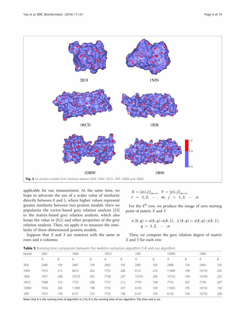
Fig. 5 Six protein models from Skolnick dataset (2B3I, 1NIN, 1RCD, 1IER, 1DBW and 1B00)

Table 5 Running time comparison between the skeleton extraction algorithm [14] and our algorithm

Model 2B3I 1NIN 1RCD 1IER 1DBW 1B00

A B A B A B A B A B A B

2B3I 2480 104 2481 104 2465 105 2481 105 2480 104 2464 105

1NIN 7472 215 8472 202 7753 208 6131 210 11809 198 10733 205

1B00 7457 208 10733 205 7738 207 10743 200 10732 194 10749 202

1RCD 7488 210 7753 208 7737 212 7759 198 7753 207 7738 207

1DBW 7456 204 11809 198 7753 207 6130 194 11825 195 10732 194

1IER 7472 199 6131 210 7753 198 6147 194 6130 194 10732 200

Notes that A is the running time of algorithm in [14], B is the running time of our algorithm. The time unit is ms

Yao et al. BMC Bioinformatics (2016) 17:131 Page 6 of 10

εmij kð Þ ¼ 1þ s kð Þj j þ t kð Þj j1þ s kð Þj j þ t kð Þj j þ s kð Þ−t kð Þj j ;

ðwhereÞ

s kð Þ ¼Xnq¼1

x0k; qð Þ; t kð Þ ¼

Xnq¼1

y0k; qð Þ;

k ¼ 1; 2; ⋅⋅⋅ ; n:

Similarly, we get the grey relation degree εijn(k) of

matrix X and Y for the kth column. Finally, we obtain thegrey relation degree of matrix X and Y by

η ¼ 12

1m

Xmk¼1

εmij kð Þ þ 1n

Xnk¼1

εnij kð Þ !

:

From the above calculation process, it is easily knownthat the grey relation degree is between 0 and 1, and thedegree indicates the high similarity of two models whenit is close to 1.

ResultsThe algorithm presented in this paper is implementedon a Intel(R) Core(TM) i3-3110 M CPU @2.5 Ghz desk-top computer with 4GB RAM running MS Windows 7.The software environment of the experiment is based onMathworks’ MATLAB R2010a.We first chose four protein models from the Protein

Data Bank [24], which are shown in Fig. 4. We alreadyknow that the 1BPD and 2BPG models are similar andthe 1WRP and 3WRP models are similar [15]. Table 1shows the results of comparing our algorithm with Qinet al’s algorithm [15] which is based on the improvedL1-medial skeleton extraction. The similarity measure-ment values of two methods are both between 0 and 1,and the more similar two protein models, the more closeto 1 their values. Our analysis method obtains a reasonablesimilarity comparison result because our value is closer to1 by comparing bold data in Table 1. In Table 2, we com-pared the execution time of two algorithm’s implementa-tions, which shows that our method runs faster thanQin et al’s algorithm [15]. We also compare our matrix-based feature descriptor to the vector-based method

1HLM 2LHB 5MBN 1CHR 5P21

1HLB 1MBA 1LH2 2MNR 1GNP

Fig. 6 Ten protein models from Chew–Kedem dataset (1HLM, 1HLB, 2LHB, 1MBA, 5MBN, 1LH2, 1CHR, 2MNR, 5P21, 1GNP)

Table 6 Similarity results for ten protein models from Fig. 6

Models 1HLM 1HLB 2LHB 1MBA 5MBN 1LH2 1CHR 2MNR 5P21 1GNP

1HLM 1.000 0.973 0.562 0.676 0.437 0.752 0.653 0.549 0.789 0.752

1HLB 0.973 1.000 0.608 0.763 0.574 0.647 0.564 0.653 0.742 0.698

2LHB 0.562 0.608 1.000 0.969 0.579 0.695 0.745 0.659 0.732 0.634

1MBA 0.676 0.763 0.969 1.000 0.614 0.713 0.697 0.705 0.720 0.744

5MBN 0.437 0.574 0.579 0.614 1.000 0.987 0.353 0.438 0.493 0.464

1LH2 0.752 0.647 0.695 0.713 0.987 1.000 0.434 0.468 0.464 0.413

1CHR 0.653 0.564 0.745 0.697 0.353 0.434 1.000 0.993 0.563 0.615

2MNR 0.549 0.653 0.659 0.705 0.438 0.468 0.993 1.000 0.595 0.685

5P21 0.789 0.742 0.732 0.720 0.493 0.464 0.563 0.595 1.000 0.981

1GNP 0.752 0.698 0.634 0.744 0.464 0.413 0.615 0.685 0.981 1.000

Yao et al. BMC Bioinformatics (2016) 17:131 Page 7 of 10

directly by SI, SGF, and the simply combined feature vectormethod ((SI + SGF)/2). The results are shown in Table 3.For two pairs of similar proteins, we find our similarityresult is more close to 1.Then, we chose three groups of protein models from

the Skolnick dataset [25], which are shown in Fig. 5. Wealready know that the 2B3I and 1NIN proteins are simi-lar because they are in the same clustering [14,25]. Forother four protein models, the 1RCD and 1IER modelsare similar, and the 1DBW and 1B00 models are similar[14,15]. We used our method to compare similarities of

these three pairs of proteins and find that they are in ac-cordance with the results of [14,15,25]. Table 4 indicatesthat two models with bold underlined data are similar(The similarity of a model with itself is always 1.000).We also compared the execution time of Li et al’s method[14] based on the improved skeleton extraction by ReebGraph and our method in Table 5. We find our method isobviously faster than the method in [14] because it doesnot need to conduct the skeleton extraction.Next, we chose 10 protein models from the Chew–

Kedem dataset [26], which are shown in Fig. 6. We have

Fig. 7 Average linkage of Skolnick's dataset by our method

Table 7 Running time comparison including searching the dataset between the skeleton extraction algorithm [14] and ouralgorithm

ModelsMethods 1HLM 2LHB 5MBN 1CHR 5P21

A 20mins 28 s 25mins 05 s 22mins 49 s 18mins 58 s 21mins 36 s

B 5mins 7mins 6mins 5mins 6mins

43 s 19 s 57 s 34 s 26 s

Note that A is the algorithm in [14] and B is our algorithm

Yao et al. BMC Bioinformatics (2016) 17:131 Page 8 of 10

known that the 1HLM and 1HLB proteins are similarbecause they are in the globin family, the 5P21 and1GNP proteins are similar because they are the alpha–beta family [26]. We computed the matrix-based greyrelation distance by using our method. The similarityresults of protein models corresponding to 10 proteinsare shown in Table 6. We find our similarity results arein agreement with the results in [26].We also demonstrate a total running time including

searching the most similar protein model for 5 proteinmodels in the Chew-Kedem dataset. In Table 7, we findour method has a fast searching speed for obtaining thesimilar protein model.To increase the robustness of our method, we added

another testing dataset as Skolnick’s dataset from R[25]for the experiment, which includes 40 proteins models.We use our method to construct the average linkage ofSkolnick's dataset in Fig. 7 and find that our result isalmost consistent with the result in R[25]. For example,the 3YPI and 1AMK proteins are in the same cluster,the 1NAT and 3CHY proteins are in the same cluster.These results are in accord with the current evolution-ary research [14,25].Finally, we compared two proteins (1BAR and 1RRO)

that have a similar shape surface but have completelydifferent secondary structure elements [13] (Fig. 8). Thealgorithm [13] based on the shape analysis by the localdiameter construction resulted in a similarity of 0.9956,which is close to 1. It falsely reflects the similarity

properties of the two proteins with different secondarystructures. Our method produced a similarity value of0.7546 which is comparatively some smaller than 1. It caninfer the non-similarity for two protein models althoughthey have similar shape surface. We conclude that ourapproach, in this specific case, improves the similarity ana-lysis for non-homologous protein models with similarshapes.

DiscussionOur method is based on the surface analysis and the ad-vantage is that the running time is fast because it doesnot need to conduct the skeleton extraction. The disadvan-tage is that it can not be applied for other protein modelssuch as protein CPK models. The advantage of the skeletonbased method is that it can be applied for both the proteinsurface (triangular mesh model) and the protein CPKmodel (point cloud representation), the disadvantage is theskeleton extraction requires a time-consuming process.

Conclusion and future workIn this paper, we propose a three-dimensional proteinmodel’s similarity analysis algorithm based on salientshape index. We first calculate the shape index (SI) andsalient geometric feature (SGF) of the protein models.And then we construct the matrix-based feature descrip-tor by SI and SGF information. Finally, we compare thesimilarity of protein models by the matrix-based grey

1BAR 1RRO

Fig. 8 1BAR and 1RRO protein models with their feature distributions

Yao et al. BMC Bioinformatics (2016) 17:131 Page 9 of 10

relation degree. Experimental results show the effective-ness of our protein similarity analysis method.Currently, we only consider the shape index (convex

and concave properties of the protein surface) and thesalient geometric feature to analyze the similarity of theprotein models. We do not take account of the physicalproperties of the protein molecules. In fact, these prop-erties such as pH, polar and non-polar, hydrophilic, alsoaffect the structure and the function of the proteinmolecules. How to combine these factors for the proteinshape similarity analysis will be our future research. Forthe clustering in our similarity analysis, we find thecluster size is normally not equal and the clustering issometimes dominated by several big clusters. The sizeof the clusters might be highly relevant in describing theglobal shape of the protein model. This also gives us aninteresting work for our future research.

Competing interestsThe authors declare that they have no competing interests.

Authors’ contributionsDeveloped the method: ZL and BY. Conceived and designed the experiments:ZL, BY, MD and MC. Analyzed the data: BY and ZL. Wrote the first draft of themanuscript: BY and ZL. Contributed to the writing of the manuscript: ZL, MDand MC. Agree with the manuscript results and conclusions: ZL, BY, MD andMC. Jointly developed the structure and arguments for the paper: BY, ZL, MDand MC. Made critical revisions and approved final version: ZL, BY, MD and MC.All the authors reviewed and approved of the final manuscript.

AcknowledgementsWe thank Prof. Stefan Heller in the school of Medicine, Stanford University,USA, for helpful discussion and suggestion. This research was supported byScientific Research Foundation of Ministry of Education of China under GrantNo. [2009]1590, Zhejiang Provincial Natural Science Foundation of China underGrant No. LY14A010032, Zhejiang Province Key Science and TechnologyInnovation Team Project (2013TD18) and Project of 521 Excellent Talent ofZhejiang Sci-Tech University.

Received: 14 September 2015 Accepted: 9 March 2016

References1. Xu SC, Li Z, Zhang SP, et al. Primary structure similarity analysis of proteins

sequences by a new graphical representation. SAR QSAR Environ Res.2014;25(10):791–803.

2. Via A, Ferre F, Brannetti B, et al. Protein surface similarities: a survey ofmethods to describe and compare protein surfaces. CMLS Cell Mol Life Sci.2000;57:1970–7.

3. Sael L, La D, Li B, et al. Rapid comparison of properties on protein surface.Proteins Struct Funct Bioinforma. 2008;73:1–10.

4. Osada R, Funkhouser T, Chazelle B, et al. Matching 3D models withshape distributions. Geneva: Proceeding of Shape Modeling International;2001. p. 07–11.

5. Horn BK. Extended Gaussian image. Proc IEEE. 1984;1671–1686.6. Ohbuchi R, Nakazawa M, Takei T. Retrieving 3D shapes based on their

appearance. Berkeley, California, USA: Proceedings of the 5th ACM SIGMMinternational workshop on Multimedia information retrieval; 2003.

7. Vranic DV, Saupe D. 3D model retrieval with spherical harmonics andmoments. London: The 23rd DAGM Symposium on Pattern Recognition,SpringVerlag; 2001. p. 392–7.

8. Hilaga M, Shinagawa Y, Komura T, et al. Topology matching for fullyautomatic similarity estimation of 3D shapes. Los Angles, California, USA:Computer Graphics, Proceedings of Annual Conference Series, ACMSIGGRAPH; 2001. p. 203–12.

9. Bronstein MM, Kokkinos I. Scale-invariant heat kernel signatures for non-rigidshape recognition. CVPR. 2010;1704–1711.

10. Foskey M, Lin MC, Manocha D. Efficient computation of a simplified medialaxis. Seattle Washington, USA: Proceedings of the Eighth ACM Symposiumon Solid Modeling and Applications; 2003. p. 96–107.

11. Du HX, Qin H. Medial axis extraction and shape manipulation of solidobjects using parabolic PDEs. Genoa: ACM Symposium on Solid Modelingand Applications; 2004. p. 25–34.

12. Morris RJ, Najmanovich RJ, Kahraman A, et al. Real spherical harmonicexpansion coefficients as 3D shape descriptors for protein binding pocketand ligand comparisons. Bioinformatics. 2005;21:2347–55.

13. Fang Y, Liu YS, Ramani K. Three dimensional shape comparison of flexibleproteins using the local-diameter descriptor. BMC Struct Biol. 2009;29(9):01–15.

14. Li Z, Qin SW, Yu ZY, et al. Skeleton-based shape analysis of protein models.J Mol Graph Model. 2014;53:72–81.

15. Qin SW, Li Z, Jin Y, et al. Shape similarity comparison of CPK models basedon improved L1-medial skeleton. SAR QSAR Environ Res. 2014;25(9):747–59.

16. Hoffman D, Singh MD. Salience of visual parts. Dep Cogn Sci. 1997;63(1):29–78.17. Bradford R, Westhead R. Improved prediction of protein–protein binding sites

using a support vector machines approach. Bioinformatics. 2008;1487–1494.18. Dyn N, Hormann K, Kim S-J, Levin D. Optimizing 3d triangulations using

discrete curvature analysis. In: Lyche T, Schumaker LL. (eds.) MathematicalMethods in CAGD, Oslo 2000, pp. 135–146 (2001).

19. Gal R, Cohen-Or D. Salient Geometric Features for Partial Shape Matchingand Similarity. ACM Trans Graph. 2006;25(1):134–8.

20. Kanungo T, Mount DM, Netanyahu NS, et al. An efficient k-means clusteringalgorithm: analysis and implementation. IEEE Trans Pattern Anal Mach Intell.2002;24(7):881–92.

21. Hu R, Fan L, Liu L. Co-segmentation of 3D shapes via subspace clustering.Eurographics Symp Geom Process. 2012;31(5):1703–13.

22. Choi S, Tappert S. A survey of binary similarity and distance measures.Cybern Inform. 2010;8(1):43–8.

23. Zhang S. Matrix absolute grey relational degree of B-Mode and itssignificance. J Grey Syst. 2012;9:135–41.

24. Protein Data Bank [http://www.rcsb.org/pdb/home/home.do].25. Pelta DA, Gonzalez JR, Vega MM. A simple and fast heuristic for protein

structure comparison. BMC Bioinforma. 2008;9(1):156–61.26. Krasnogor N, Pelta DA. Measuring the similarity of protein structure by means

of the universal similarity metric. BMC Bioinforma. 2004;20(7):1015–21.

• We accept pre-submission inquiries

• Our selector tool helps you to find the most relevant journal

• We provide round the clock customer support

• Convenient online submission

• Thorough peer review

• Inclusion in PubMed and all major indexing services

• Maximum visibility for your research

Submit your manuscript atwww.biomedcentral.com/submit

Submit your next manuscript to BioMed Central and we will help you at every step:

Yao et al. BMC Bioinformatics (2016) 17:131 Page 10 of 10