three essays in industrial organization
TRANSCRIPT

Three Essays in Industrial Organization
by
Matthew R. Backus
A dissertation submitted in partial fulfillmentof the requirements for the degree of
Doctor of Philosophy(Economics)
in The University of Michigan2012
Doctoral Committee:
Professor Daniel A. Ackerberg, ChairProfessor Francine LafontaineProfessor Scott E. PageAssistant Professor Jeremy FoxAssistant Professor Natalia Lazzati

c© Matthew R. Backus 2012.All Rights Reserved.

To my parents
ii

ACKNOWLEDGEMENTS
A special thanks to my dissertation committee for their invaluable encouragement and comments:
Dan Ackerberg(Chair), Jeremy Fox, Francine Lafontaine, and Natalia Lazzati, and Scott Page. Also
special thanks to William Adams, Randy Becker, Sasha Brodski, Ying Fan, Shawn Klimek, Kai-Uwe
Kuhn, Greg Lewis, and Jagadeesh Sivadasan for thoughtful comments. Chapter 1 of this dissertation
was written while I was a Special Sworn Status researcher of the US Census Bureau at the University
of Michigan Research Data Center. Any opinions and conclusions expressed herein are those of the
author and do not necessarily represent the views of the U.S. Census Bureau. All results have been
reviewed to ensure that no confidential information is disclosed. All remaining errors are my own.
iii

TABLE OF CONTENTS
DEDICATION . . . . . . . . . . . . . . . . . . . . . . . . . . . . . . . . . . . . . . . . . . . ii
ACKNOWLEDGEMENTS . . . . . . . . . . . . . . . . . . . . . . . . . . . . . . . . . . . iii
LIST OF FIGURES . . . . . . . . . . . . . . . . . . . . . . . . . . . . . . . . . . . . . . . vi
LIST OF TABLES . . . . . . . . . . . . . . . . . . . . . . . . . . . . . . . . . . . . . . . . vii
CHAPTER
I. Introduction . . . . . . . . . . . . . . . . . . . . . . . . . . . . . . . . . . . . . . . 1
II. Why is Productivity Correlated with Competition? . . . . . . . . . . . . . . 3
2.1 Introduction . . . . . . . . . . . . . . . . . . . . . . . . . . . . . . . . . . . . 32.2 Data and Measurement . . . . . . . . . . . . . . . . . . . . . . . . . . . . . . 5
2.2.1 The Ready-Mix Concrete Industry . . . . . . . . . . . . . . . . . . 52.2.2 Sample Inclusion . . . . . . . . . . . . . . . . . . . . . . . . . . . . 62.2.3 Market Definition . . . . . . . . . . . . . . . . . . . . . . . . . . . . 72.2.4 Measuring Competition . . . . . . . . . . . . . . . . . . . . . . . . 72.2.5 Productivity Measurement . . . . . . . . . . . . . . . . . . . . . . . 8
2.3 The Productivity Effect of Competition . . . . . . . . . . . . . . . . . . . . . 92.4 X-Inefficiency . . . . . . . . . . . . . . . . . . . . . . . . . . . . . . . . . . . 112.5 Dynamic Selection . . . . . . . . . . . . . . . . . . . . . . . . . . . . . . . . . 122.6 Methodology and Estimation . . . . . . . . . . . . . . . . . . . . . . . . . . . 14
2.6.1 The Quantile Approach . . . . . . . . . . . . . . . . . . . . . . . . 142.6.2 The Selection Correction Approach . . . . . . . . . . . . . . . . . . 16
2.7 Conclusion . . . . . . . . . . . . . . . . . . . . . . . . . . . . . . . . . . . . . 20
III. General Comparative Statics for Industry Dynamics in Long-Run Equi-librium . . . . . . . . . . . . . . . . . . . . . . . . . . . . . . . . . . . . . . . . . . . 37
3.1 Introduction . . . . . . . . . . . . . . . . . . . . . . . . . . . . . . . . . . . . 373.2 Model . . . . . . . . . . . . . . . . . . . . . . . . . . . . . . . . . . . . . . . . 38
3.2.1 Idiosyncratic Types . . . . . . . . . . . . . . . . . . . . . . . . . . . 383.2.2 Stage Game . . . . . . . . . . . . . . . . . . . . . . . . . . . . . . . 393.2.3 Entry and Exit . . . . . . . . . . . . . . . . . . . . . . . . . . . . . 403.2.4 Timing and Dynamics . . . . . . . . . . . . . . . . . . . . . . . . . 40
3.3 Equilibrium . . . . . . . . . . . . . . . . . . . . . . . . . . . . . . . . . . . . 413.4 Comparative Statics . . . . . . . . . . . . . . . . . . . . . . . . . . . . . . . . 44
3.4.1 Fixed Costs of Entry . . . . . . . . . . . . . . . . . . . . . . . . . . 453.4.2 Market Size . . . . . . . . . . . . . . . . . . . . . . . . . . . . . . . 46
iv

3.5 Conclusion . . . . . . . . . . . . . . . . . . . . . . . . . . . . . . . . . . . . . 483.6 Appendix . . . . . . . . . . . . . . . . . . . . . . . . . . . . . . . . . . . . . . 49
IV. An Estimable Demand System for a Large Auction Platform Market (withGregory Lewis) . . . . . . . . . . . . . . . . . . . . . . . . . . . . . . . . . . . . . 58
4.1 Introduction . . . . . . . . . . . . . . . . . . . . . . . . . . . . . . . . . . . . 584.2 Model . . . . . . . . . . . . . . . . . . . . . . . . . . . . . . . . . . . . . . . . 61
4.2.1 Environment . . . . . . . . . . . . . . . . . . . . . . . . . . . . . . 614.2.2 Analysis . . . . . . . . . . . . . . . . . . . . . . . . . . . . . . . . . 63
4.3 Nonparametric Identification . . . . . . . . . . . . . . . . . . . . . . . . . . . 694.3.1 Example . . . . . . . . . . . . . . . . . . . . . . . . . . . . . . . . . 694.3.2 Formal Result . . . . . . . . . . . . . . . . . . . . . . . . . . . . . . 71
4.4 Estimation Strategy . . . . . . . . . . . . . . . . . . . . . . . . . . . . . . . . 724.4.1 Step 1: Estimate transitions, exit and payments . . . . . . . . . . . 734.4.2 Nonparametric Approach Step 2: Recover valuations . . . . . . . . 744.4.3 Semiparametric Approach Step 2a: Estimate bid function . . . . . 754.4.4 Semiparametric Approach Step 2b: Match Moments . . . . . . . . 754.4.5 Characteristic Space Approach . . . . . . . . . . . . . . . . . . . . 77
4.5 Monte Carlo . . . . . . . . . . . . . . . . . . . . . . . . . . . . . . . . . . . . 784.6 Conclusion . . . . . . . . . . . . . . . . . . . . . . . . . . . . . . . . . . . . . 814.7 Appendix . . . . . . . . . . . . . . . . . . . . . . . . . . . . . . . . . . . . . . 81
V. Conclusion . . . . . . . . . . . . . . . . . . . . . . . . . . . . . . . . . . . . . . . . 89
BIBLIOGRAPHY . . . . . . . . . . . . . . . . . . . . . . . . . . . . . . . . . . . . . . . . . 90
v

LIST OF FIGURES
Figure
2.1 County Map of the USA . . . . . . . . . . . . . . . . . . . . . . . . . . . . . . . . . 272.2 CEA Map of the USA . . . . . . . . . . . . . . . . . . . . . . . . . . . . . . . . . . 282.3 Allocative vs. Productive Efficiencies . . . . . . . . . . . . . . . . . . . . . . . . . . 292.4 Value Function Response to Change in Market Size. . . . . . . . . . . . . . . . . . 302.5 Predicted effect of two narratives on productivity residual distribution. . . . . . . . 312.6 Effect of the number of ready-mix concrete firms on deciles of the productivity
residual distribution by CEA. Corresponds to models (1) and (2). . . . . . . . . . . 322.7 Effect of HHI (calculated using firms) on deciles of the productivity residual distri-
bution by CEA. Corresponds to models (3) and (4). . . . . . . . . . . . . . . . . . 332.8 Effect of the number of ready-mix concrete establishments on deciles of the produc-
tivity residual distribution by CEA. Corresponds to models (5) and (6). . . . . . . 342.9 Effect of HHI (calculated using establishments) on deciles of the productivity resid-
ual distribution by CEA. Corresponds to models (7) and (8). . . . . . . . . . . . . 353.1 Industry in Equilibrium: Recall Ψ(φ) =
∫v(φ′, µ;D)dF (φ′|φ) is the continuation
value for a firm of type φ today. Condition E2 requires that Ψ(φ) pass through thepoint (φE ,cF ), while condition E3 gives x∗ at the Y-intercept of the function. . . . 55
3.2 Decrease in Entry Costs: Let cf1 > cf2 . The reduction spurs entry, which drivesprofits down for all types. The new continuation value function Ψ2(φ) is smallerthan Ψ1(φ), and valued cf2 at φE . The exit threshold x∗ rises, spurring higherturnover and average type. . . . . . . . . . . . . . . . . . . . . . . . . . . . . . . . . 56
3.3 Increase in Market Size: Let D1 < D2. The increase in demand raises profits, inparticular for higher types. The higher profits spur entry, in turn reducing prof-its, especially for lower types. Combined, these countervailing effects push Ψ2(φ)counterclockwise around the original Ψ1(φ), pivoting around (φE , cf ). . . . . . . . 57
4.1 Monte Carlo Simulation: The figure shows the true and estimated marginal densityof valuations for product 1 for a randomly chosen Monte Carlo simulation of 500auctions with specification E. . . . . . . . . . . . . . . . . . . . . . . . . . . . . . . 80
vi
LIST OF TABLES
Table
2.1 Summary Statistics by CEA . . . . . . . . . . . . . . . . . . . . . . . . . . . . . . . 222.2 OLS Results . . . . . . . . . . . . . . . . . . . . . . . . . . . . . . . . . . . . . . . . 222.3 Instrumental Variables Results . . . . . . . . . . . . . . . . . . . . . . . . . . . . . 232.4 Decile Effects (β
(k)d ) . . . . . . . . . . . . . . . . . . . . . . . . . . . . . . . . . . . 24
2.5 Instrumental Variables with Selection Correction Results . . . . . . . . . . . . . . . 252.6 Comparison of Results . . . . . . . . . . . . . . . . . . . . . . . . . . . . . . . . . . 262.7 Probit Results . . . . . . . . . . . . . . . . . . . . . . . . . . . . . . . . . . . . . . . 364.1 Monte Carlo Results: Simple Model . . . . . . . . . . . . . . . . . . . . . . . . . . 864.2 Monte Carlo Results: Forward-Looking Model . . . . . . . . . . . . . . . . . . . . . 874.3 Monte Carlo Results: Backward-Looking Model . . . . . . . . . . . . . . . . . . . . 88
vii

CHAPTER I
Introduction
The three chapters of this dissertation are unified by two common interests: first, the modeling
of economic agents in an explicitly dynamic setting in order to capture, whether empirically or
analytically, features of their decision-making that depend on an endogenous, changing future and
second, an interest in deriving results, whether empirical or analytic, from models that depend on
economic rather than parametric assumptions.
Chapter 1 seeks an explanation for the oft-observed correlation between plant-level productivity
measures and market-level indexes of competition. The set of potential explanations can be divided
into two econometrically separable bins: X-inefficiency and dynamic selection. The former is a
plant-level treatment effect of competition and the latter is a selection story in which larger, more
competitive markets select more aggressively on productivity type. The distinction is identified both
by mechanism and by outcome: by mechanism, a nonparametric selection correction controls for
the effect of dynamic selection; by outcome, one compares the predicted and the actual effects on
quantiles of the market-level distribution of productivity residuals. The ready-mix concrete industry,
using data from the US Census of Manufactures, is a natural setting to apply these methods. Varia-
tion in competition at the local market level is driven by exogenous changes in demand for ready-mix
concrete. Both identification strategies point to X-inefficiency as the dominant explanation, raising
important questions about within-plant responses to competition.
Chapter 2 considers the set of comparative statics that can be obtained from industry dynam-
ics models without writing down a parametric model of the stage game. Results are obtained for
average type and turnover with respect to changes in market size and entry cost. Those for mar-
ket size depend on a simple and economically meaningful increasing differences assumption on the
relationship between firm type and competition. The generality of these results is important for
the booming literature that applies parametric variations of industry dynamics models to match
1

empirical stylized facts of plant-level production data and the effects of trade policy.
Chapter 3 constructs a model of repeated second-price auctions in which bidders are persistent
and have multidimensional private valuations. In this setting, equilibrium bids are shaded by the
endogenous option value of losing to bid another day. We prove existence of this equilibrium and
characterize the ergodic distribution of types. Having developed a demand system, we show that it is
non-parametrically identified from panel data. Relatively simple nonparametric and semiparametric
estimation procedures are proposed and tested by Monte Carlo simulation. The analysis highlights
the importance of both dynamic bidding strategies and panel data sample selection issues when
analyzing these markets.
2
CHAPTER II
Why is Productivity Correlated with Competition?
2.1 Introduction
There is a perennial paper in the productivity literature which presents the following empirical
result, updated for contemporary innovations in attitudes towards data and econometrics: firms
that are in more competitive markets are also more efficient. In the era of cross-sectional, cross-
industry regressions, the correlation was straightforward to measure (Green and Mayes (1991) Caves
and Barton (1990)). As panel methods became more prominent, the empirical result stood out
in still more clarity (Hay and Liu (1997), Nickell (1996), Pavcnik (2002)). Finally, when cross-
industry regressions became suspect, though finding an appropriate industry and instrument became
a challenge, the correlation was robust (Berger and Hannan (1998), Syverson (2004), Schmitz (2005),
Dunne, Klimek, and Schmitz (2010)).
The existence of a correlation between competition and productivity is significant both for anti-
trust as well as trade policy. As Williamson (1968) noted in the case of horizontal merger evaluation,
for deadweight loss to outweigh alleged productive synergies the estimated percentage change in
price would have to be several times larger than the percentage efficiency gain. Efficiency losses
from market concentration, however, which affect not only all firms in the market but operate on
infra-marginal sales, could potentially overturn that result. If measurable, these rectangles may be a
much stronger argument for worrying about mergers than deadweight loss triangles, famously found
to be so diminutive by Harberger (1954). Moreover, trade economists have been quick to adopt
measured efficiency gains as one of the central arguments for gains from trade, a Pantheon formerly
dominated by allocative efficiencies and Ricardo’s argument from comparative advantage.
No consensus exists, however, regarding the explanation for such a correlation. There are two
main hypotheses: First, that competition has a direct effect on productivity. This hypothesis was
originally introduced as a black box under the name ”X-inefficiency” by Leibenstein (1966) and
3

has since received considerable theoretical development. A second hypothesis has emerged from
the trade literature on productivity gains from trade liberalization: that more competitive markets
select more aggressively on productivity. Even in the absence of a direct causal relationship, this
implies that the selected sample in more competitive markets will be, on average, more productive
than that in less competitive markets.1 The two hypotheses will be referred to here as X-inefficiency
and dynamic selection.2
The conflation of these two effects is not unknown, and some of the papers documenting the
correlation between competition and productivity have included reduced-form efforts to control for
dynamic selection. Pavcnik (2002) applies Olley and Pakes (1996) to obtain productivity residuals,
and then uses a regression framework with exit dummies to control for the selection effect. Alterna-
tively, Schmitz (2005) adopts a decomposition approach to measure the relative effects of exit and
within-firm change. Both papers find evidence in favor of the within-firm X-inefficiency story.
This paper endeavors to disambiguate the two stories in a way that is structurally consistent and
requires minimal appeal to parametric form beyond the original derivation productivity residuals.
Identification is formulated two way– first, bys thinking about the effect on the ergodic distribution
of types; though the predictions of X-inefficiency on the distribution of types is ambiguous, the
dynamic selection story implies the correlation of productivity quantiles and competition should
be decreasing in quantile, since it operates primarily on the left tail. Second, an explicit model of
the firm’s decision problem is formulated in order to derive a selection correction procedure which
isolates the effect of X-inefficiency by controlling completely for dynamic selection. While the first
approach has the appealing feature of offering a direct visual test, the latter is used to generate
numerical estimates of the relative contribution of the two stories. Both confirm the dominance of
X-inefficiency.
The natural setting for applying these identification techniques is ready-mix concrete. One of the
difficulties of studying the correlation between competition and productivity is generating sufficient
cross-sectional variance in competitive structure. High transportation costs make ready-mix concrete
1This is related, but not identical, to the selection issue treated in the third stage of Olley and Pakes’s (1996)structural production function estimator. In their paper there is only one market, and therefore market structure isfully controlled for by allowing the propensity score estimator to vary nonparametrically in time. Even given consistentestimator of the productivity residual, however, reduced-form estimates of the within-firm increase in productivitywill be influenced upwards by dynamic selection, as survivors in an increasingly competitive market are more likelyto have had a favorable innovation in productivity.
2A third hypothesis emerges if the object of interest is revenue-weighted average productivity; more competitivemarkets may better allocate demand to higher productivity firms, a hypothesis that comes out strong in Olleyand Pakes (1996). This paper pre-empts the third hypothesis by focusing on unweighted productivity, not becauseallocation is unimportant, but because it is beyond the scope of the paper– the focus here is to disambiguate theempirical consequences of X-inefficiency and dynamic selection. Moreover, due to data exclusion issues describedbelow, the data is poorly suited to measuring the reallocation effect.
4
markets local in character; these local markets permit the measurement of just such variance. Second,
the availability of homogeneous output measures in physical, rather than revenue terms, allows one
to estimate physical productivity entirely separately from market power. This paper builds on
Syverson’s (2004) pioneering study of productivity dispersion in ready-mix concrete, though here
the first rather than the second moment is under consideration,3 and this first moment is leveraged
to examine the underlying model. Also closely related is Collard-Wexler (2011), which studies the
determinants of establishment survival in ready-mix concrete markets.
There is also an extensive related literature on the use of decomposition methods in the study of
changes in aggregate productivity. Here, a regression framework is used instead of decomposition for
two reasons: to begin with, the objective is to take advantage of cross-sectional variation in order to
map the changes in productivity onto a continuous explanatory variable, an index of competition.
Decomposition methods are most apposite to the study of time-series variation and discrete policy
changes, as in Olley and Pakes (1996). Moreover, the dynamic selection story posited as an alterna-
tive to X-inefficiency is also a potential source of bias which would tend to overstate the within-firm
share of the change in productivity. At the end of the day, however, little evidence is found for the
dynamic selection effect, which should in turn offer reassurance on the use of decomposition methods
in productivity analysis.
Section 2 describes the ready-mix concrete industry, the data used, and the measurement issues
associated with studying productivity, spatially defined markets, and competition indexes. Section
3 captures the correlation between competition and productivity with a reduced-form instrumental
variables approach. In section 4 and 5 the theoretical foundations for the two effects conflated in that
correlation are explored, and section 6 expounds on and implements two strategies for separating
them econometrically. Section 7 concludes.
2.2 Data and Measurement
2.2.1 The Ready-Mix Concrete Industry
This paper uses US Census of Manufactures data for the ready-mix concrete industry (SIC 3273)
for years 1982, 1987, and 1992. Ready-mix concrete is a mixture of cement, water, gravel, and
a handful of chemical additives. Stockpiles of these materials are stored at the plant, mixed on
demand, and loaded in liquid form into a ready-mix concrete truck for delivery at the construction
3Syverson (2004) is built on a variant of the dynamic selection story and finds an average productivity effect aswell, however notes (see footnote 6) that this effect would be conflated with X-inefficiency, and that it is beyond thescope of that paper to disentangle the two effects.
5

site, where the concrete is poured.
The liquid mixture begins to set as soon as it is loaded into the ready-mix concrete truck; besides
the potential for wasted materials, there are costs associated with removing hardened concrete from
the inside of the drums of ready-mix concrete trucks. These two factors both contribute to the
high transportation costs which render this industry markedly local in scope. Geographic market
definition is discussed below, however it is this uniquely local character which makes ready-mix
concrete such an attractive industry for study; in order to measure the effect of competition on
productivity, one requires variation in competitive structure. This is difficult to obtain for most
manufacturing industries, which compete in an increasingly integrated world market.
A second important feature of the industry is the homogeneity of the output. Though the compo-
sition of the chemical additives may differ some by application, this is thought to generate very little
product differentiation. For this reason, in the years 1982, 1987, and 1992 the Products Supplement
to the Census of Manufactures includes output data in cubic yards, which obviates many of the
concerns that would accompany the use of deflated revenue in estimating productivity. Using phys-
ical output to measure productivity is especially apposite to this application because productivity
residuals based on revenue measures will be reflect market-level and idiosyncratic demand shocks
through firms’ mark-ups, generating a spurious correlation between competition and productivity. 4
The Census of Manufactures offers extensive data on inputs of production which are used to
estimate productivity residuals, as discussed below. For more extensive discussion of the data and
the ready-mix concrete industry, the reader is referred to Syverson (2008).
2.2.2 Sample Inclusion
There are over five thousand ready-mix concrete establishments observed by the Census of Man-
ufactures in each year of my sample. Unfortunately, roughly one-third of these establishments are
”administrative records” establishments; that is, small enough to be exempt from completing census
forms. Data for these is a combination of administrative records from other agencies and imputation,
and is therefore unusable for calculating productivity residuals.
A small handful of establishments are extensively diversified and operate in multiple SIC codes.
Here they are excluded if less than fifty percent of their total sales is composed of ready-mix concrete.
For diversified establishments which survive this exclusion, inputs devoted to ready-mix concrete are
approximated by multiplying the fraction of sales from ready-mix concrete by the conflated input
4This is less of an issue to the extent that one finds a positive correlation between competition and productivity;mark-ups in the measurement error of productivity would be negatively correlated with competition and thereforemerely attenuate the result.
6

variable. Finally, the establishment-level price of a cubic yard of concrete is calculated by dividing
revenues by quantity, and a small number of firms with extremal values are excluded from the
sample.
It is important to note that while these establishments are excluded for regressions that depend
on estimates of the productivity residuals, they are not excluded in the calculation of market-level
variables– in particular the competition indexes discussed below in section 2.4.
2.2.3 Market Definition
This paper employs the Component Economic Area (CEA) market definition to study ready-mix
concrete markets. CEAs are a complete and mutually exclusive categorization of the nation’s over
three thousand counties into 348 economic markets5. In contrast with the sometimes arbitrary size
and shapes of counties (see Figure 2.1), the typical CEA is defined first by the identification of
an economic node, and then the assignment of non-nodal counties to economic nodes by newspaper
readership and traffic commuting patterns (see Figure 2.2). Johnson and Kort (2004) offers more
discussion of the assignment of counties to CEAs, and Syverson (2004), which pioneered the use of
CEAs in the study of ready-mix concrete, offers still more motivation for their use.
2.2.4 Measuring Competition
In a Markov-perfect industry dynamics model with full information (e.g., Ericson and Pakes
(1995)), the competitive structure of the market enters the payoff and value functions of the firm
through a high-dimensional state variable which includes the type of every active firm in the market.
As the explicit inclusion of such a variable is infeasible for empirical work, two indexes are constructed
which capture the salient features of the state of the market.
On the extensive margin, the size of the market is captured by the number of ready-mix concrete
firms per square mile. Informally, the more ready-mix concrete firms there are in a fixed geographic
space, the more substitutable they are, and therefore the more intense the competition between
them.
The second measure is meant to capture the intensive margin. The Herfindal-Hirschman Index
is constructed from the revenue of active firms. Though this variable will be negatively correlated
with the number of firms, it also captures the allocation of demand between firms, and therefore
reflects the dispersion of firm types.6
5The number of CEAs was revised to 344 in 2004, however this paper employs the pre-2004 CEA definitions.6Here firm type is meant to be interpreted very loosely. One firm may be dominant because it has idiosyncratically
low costs; alternatively, it may have strong idiosyncratic demand, e.g. informal ties with contractors.
7

Both of these measures can be sensibly computed using either establishments or firms as the
unit of observation. This paper presents results for both. Summary statistics for these competition
indexes can be found in Table 2.1. As noted above, the calculation of the competition indexes
includes the administrative record and diversified firms discussed in section 2.2.
2.2.5 Productivity Measurement
Establishment-level productivity, denoted by ωit, is measured as the additive residual from a
Cobb-Douglas gross output production function in log form. That is,
(2.1) ωit = yit − αltlit − αk(s)tk(s)it − αk(e)tk
(e)it − αmtmit − αeteit
–where yit is output, lit is labor, k(s)it is capital in structures, k
(e)it is equipment capital, mit is
materials, and eit is energy. Inputs and output are in logs. Input elasticities αt are estimated using
industry level cost shares, which are calculated from the NBER productivity database (therefore
indirectly, from the Census of Manufacturers).7 Equipment and structure capital shares are con-
structed using reported stocks multiplied by rental rates for the two-digit industry from the BLS.8
In what follows, these productivity residuals will be the dependent variables in a series of regres-
sions designed to look for- and to explain- the correlation between competition and productivity.
Two assumptions employed in the derivation of these residuals are suspect: first, constant returns to
scale is assumed and has been tested in Syverson (2004).9 Second, the hypothesis of X-inefficiency
may be conflated with optimization failure. As discussed below, this paper remains agnostic as to
the particulars, but models of X-inefficiency have been developed which are not inconsistent with
optimal input choice. Still, one way to deal with this would be to wrap the entire selection correc-
tion procedure described below into a one-stage structural production function estimator based on
Ackerberg, Caves, and Frazer (2006)10. This paper obtains the productivity residuals in a first stage
for the sake of expositional clarity.
7This contains an implicit assumption of constant returns to scale. Syverson (2004) tests this assumption for theready-mix concrete industry, and finds the results supportive.
8For a discussion of the use of index methods for estimating TFP with CMF data, see Syverson (2004).9In the next draft of this paper, the assumption is tested by regressing ωit on the predicted level of output and cit,
both instrumented by the set of demand shifters. Results for this robustness check are still pending disclosure reviewwith the US Census Bureau.
10This exercise would require additional timing assumptions on the choice of materials in order to avoid the collinear-ity problems described in Bond and Sderbom (2005). For instance, one might assume that materials are chosen atsome point in time just prior to t, following Ackerberg, Caves, and Frazer’s (2006) assumptions on the choice of labor.This is not implausible; one can think of material usage as being dictated by contracts which are agreed upon priorto production. However, one additional advantage of the fully structural approach would be the incorporation of anunobservable (to the firm) idiosyncratic productivity shock.
8
2.3 The Productivity Effect of Competition
Taking a reduced-form approach to measuring the relationship between competition and produc-
tivity, the following regression is standard:
(2.2) ωit = β0 + βccm(i)t + εit
This regression is constitutive of the literature on competition and productivity, and carries
hefty baggage: The first challenge is to obtain sufficient variation in competitive structure. One
solution, now largely outmoded, is to run cross-industry regressions. This paper avoids the problems
associated with cross-industry regressions by focusing on an industry with many local markets.
Second, to the extent that productivity is estimated using deflated revenue as output, the error
introduced will be correlated with the competition index via mark-ups. Foster, Haltiwanger, and
Syverson (2008) identify a set of industries (including ready-mix concrete) for which both physical
and revenue output data are available, and explore the relationship. As in their work, this problem
is obviated by the availability of physical output data for ready-mix concrete.11
OLS results for (2.2) are presented in Table 2.2. For all four competition indexes there is a pos-
itive and statistically significant correlation between competition and productivity. The regressions
using count indexes are run in log-log form, and therefore the coefficients βOLS can be interpreted
as elasticities of output with respect to competition12. The HHI indexes are scaled between zero
and one and unlogged; the coefficient is therefore interpreted as the efficiency difference between two
extrema: complete dispersion and absolute monopoly.
An obvious concern with these results is the endogeneity of competition. The presence of high-
type firms will likely discourage entry, and therefore generate a non-causal correlation between
concentration and productivity which biases the estimates.13 One strategy for dealing with this
problem is to identify an exogenous regulatory shock to the level of competition. In the trade
literature, liberalization of trade regulations provides extensive data on this front; Olley and Pakes
11In the next draft of this paper, results will be also available for all of the estimation results with productivitycalculated using revenue output, rather than physical output. It is interesting to know whether, as a simple modelwould predict, the use of revenue measures attenuates the results, and whether the methods can be applied to industrieswhere physical output data is unavailable. These results are pending disclosure review at the US Census Bureau.
12It is important to remember that the percentage change interpretation of elasticities is based on consideration ofsmall changes, and therefore breaks down here for some common and interesting cases, e.g. the addition of a secondcompetitor in a low-demand CEA– a 100% increase in the number of competitors.
13Nickell (1996) notes that this source of endogeneity, like that stemming from the use of revenue-based productivitymeasures, works in the ”right direction” in that it attenuates any positive correlation between competition andproductivity.
9

(1996) use the forced breakup of a monopsonistic downstream firm. There are limitations to this
approach. On the one hand, they are often one-shot or at best finitely staged events. Moreover,
because they are typically common shocks, they are absorbed entirely by time effects, and therefore
conflated with other sources of variation. To the extent that the shocks are not common, the
identifying comparison is made either across industry or across geographic regions. An alternative
approach, pioneered by Syverson (2004), builds on the insight of Sutton (1991) that competition
in the long run is dictated by market fundamentals. A market-level demand shifter is an eligible
instrument generating exogenous variation in competitive structure. Higher demand encourages
entry, and more entry implies lower transportation costs and increased substitutability.
This paper employs a number of instruments to capture the level of demand for ready-mix
concrete: construction employment (SIC 15), the total number of residential building permits issued,
single-family building permits, five or more family building permits, and local government highway
and road expenditure.14 Summary statistics are presented in Table 1. In the regressions which
follow, however, the instruments are divided by area, in square miles, to approximate the density of
demand and then logged.
More firms in a finite geographic space implies more substitutability, and therefore relevance to
our indexes of competition. Exogeneity is maintained by arguing that ready-mix concrete typically
comprises a small portion of a construction budget, and therefore the decision whether to build is
unlikely to reflect variation in mark-ups stemming from competitive structure. Using these demand
shifters to instrument for the endogenous index cm(i)t, the following regression is run:
(2.3) ωit = β1 + βIV cm(i)t + εit
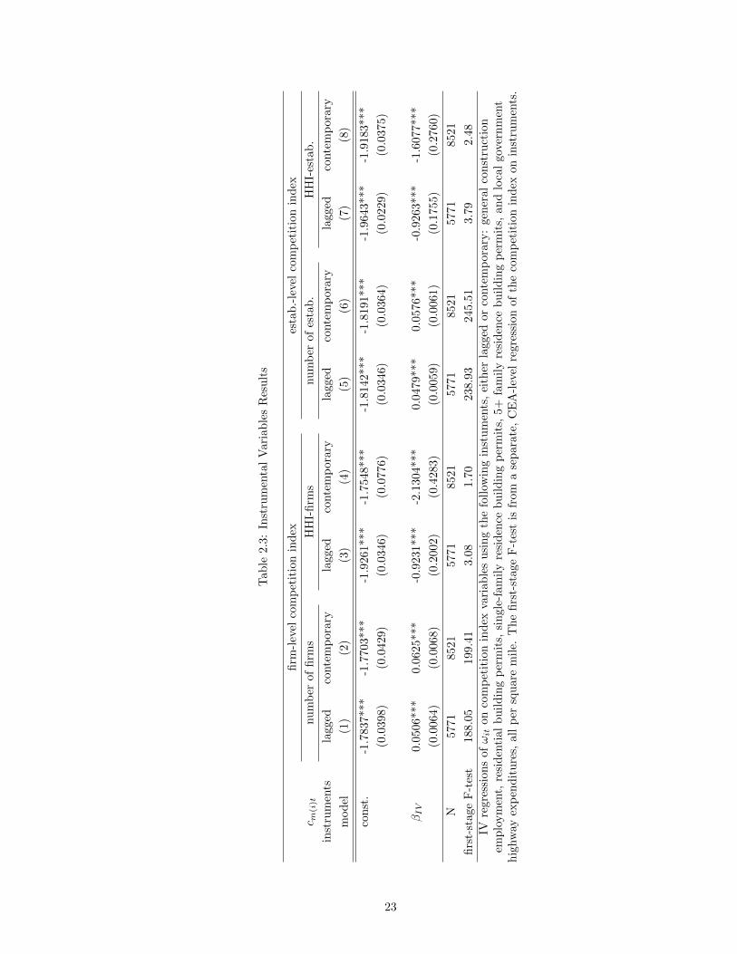
Results for the baseline IV model under a variety of specifications are presented in Table 2.3. For
all specifications, a strong and robust effect of competition is found on productivity. For comparison,
the standard of deviation of ωit over the period of the sample is found to be 0.2768. The first-stage
F-statistics are presented at the bottom of the table, and suggest some concern for the strength of the
instruments at predicting the endogenous regressor for those specifications using HHI. The results
are rather stronger than those obtained by OLS in Table 2.2, which seems to support Nickell’s (1996)
argument that the endogeneity bias will attenuate, rather than exaggerate, the positive correlation.
The results are reported for both lagged and contemporary instruments, for comparison with
14Construction employment is calculated directly from the LBD. The last four instruments are taken from the USACounties data available online from the US Census Bureau.
10
the selection correction model presented in section 6, where the importance of the distinction will
be apparent. Though strong, the results have no structural interpretation. They conflate the direct
effect of X-inefficiency with the bias induced by dynamic selection. The next two sections expand
on the theory behind these two stories, with the ultimate goal of disambiguating them empirically.
2.4 X-Inefficiency
The term X-inefficiency was coined by Leibenstein (1966) and born to immediate controversy.
The concept was originally posed as a counterpoint contemporary optimal choice theory, which
sparked a heated debate and some very colorfully titled papers (Stigler (1976), Leibenstein (1978)).
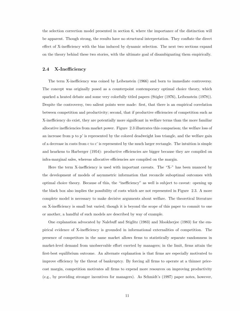
Despite the controversy, two salient points were made: first, that there is an empirical correlation
between competition and productivity; second, that if productive efficiencies of competition such as
X-inefficiency do exist, they are potentially more significant in welfare terms than the more familiar
allocative inefficiencies from market power. Figure 2.3 illustrates this comparison; the welfare loss of
an increase from p to p’ is represented by the colored deadweight loss triangle, and the welfare gain
of a decrease in costs from c to c’ is represented by the much larger rectangle. The intuition is simple
and hearkens to Harberger (1954): productive efficiencies are bigger because they are compiled on
infra-marginal sales, whereas allocative efficiencies are compiled on the margin.
Here the term X-inefficiency is used with important caveats. The “X-” has been nuanced by
the development of models of asymmetric information that reconcile suboptimal outcomes with
optimal choice theory. Because of this, the “inefficiency” as well is subject to caveat: opening up
the black box also implies the possibility of costs which are not represented in Figure 2.3. A more
complete model is necessary to make decisive arguments about welfare. The theoretical literature
on X-inefficiency is small but varied; though it is beyond the scope of this paper to commit to one
or another, a handful of such models are described by way of example.
One explanation advocated by Nalebuff and Stiglitz (1983) and Mookherjee (1983) for the em-
pirical evidence of X-inefficiency is grounded in informational externalities of competition. The
presence of competitors in the same market allows firms to statistically separate randomness in
market-level demand from unobservable effort exerted by managers; in the limit, firms attain the
first-best equilibrium outcome. An alternate explanation is that firms are especially motivated to
improve efficiency by the threat of bankruptcy. By forcing all firms to operate at a thinner price-
cost margin, competition motivates all firms to expend more resources on improving productivity
(e.g., by providing stronger incentives for managers). As Schmidt’s (1997) paper notes, however,
11

the effect depends strongly on parametric assumptions. More recently, Raith (2003) offers an ex-
planation that hinges on market dynamics. He identifies two competing effects; a business stealing
effect which increases returns to improving productivity when competition is more intense, and a
scope effect, which decreases the returns to improving productivity when competing firms have low
prices. He shows that while these effects cancel out in a static model, endogenous exit makes the
prediction unambiguous: the business stealing effect dominates, and firms have more incentive to
improve productivity in more competitive markets.
The set of explanations described here is both rich and incomplete; moreover, is likely that at
this level of analysis, the particular industry and institutional context is likely to play an important
role. Rather than advocating a particular explanation, the argument here will remain agnostic,
characterizing by X-inefficiency any story such that, at equilibrium, the production function can be
represented as if the competitive structure of the market were an input of production:
(2.4) yit = f(xit, cm(i)t) + φit
The generality here highlights the common and essential feature of stories of X-inefficiency which
will be econometrically identified: the direct, causal effect of competition on productivity. If one
could take a firm out of a less competitive market and put it into a more competitive one, X-
inefficiency implies that the firm would experience an increase in productivity.
2.5 Dynamic Selection
The dynamic selection effect is a story that has gained traction in the international trade lit-
erature and owes its intellectual heritage to Melitz’s (2003) innovative extensions to the general
industry dynamics model of Hopenhayn (1992a). In contrast to the direct productivity effect that
drives X-inefficiency, dynamic selection is a story about the selection of the set of firms that are
observed in equilibrium. Unprofitable firms exit, spurring entry of new firms. If the break-even
threshold is stricter in more competitive markets, it will be the case that the set of firms which
survive this stricter survival rule will be, on average, more productive.
Three essential features drive models which explain dynamic selection: Idiosyncratic types, an
unlimited pool of ex-ante identical entrants, and endogenous exit. Particularly apposite to ready-
mix construction, Syverson (2004) presents a two-stage entry game in which entrants pay a fixed
12

cost to learn their marginal costs, exit if the costs are too high, and then compete for the business of
consumers arranged on a circle with transportation costs. Though the model does not capture the
repeated play of other industry dynamics approaches, the payoff is the explicitly spatial character
of stage-game competition. As demand density on the circle increases, more firms enter, and the
exit cutoff becomes stricter, in turn lowering average observed marginal cost. Melitz and Ottaviano
(2008), exemplary of the trade literature approach, employs parametric assumptions and structural
assumptions on demand and the form of competition in exchange for closed-form analytic compar-
ative statics. As in Hopenhayn (1992a), firm types evolve according to a Markov process, and firms
exit should the expected discounted value of future profits ever become negative. That exit threshold
is shown to be stricter in larger markets. Finally, Backus (2011) generalizes the Hopenhayn (1992a)
approach to derive comparative statics without parametric restrictions or assumptions on the form of
competition. In comparison with Melitz and Ottaviano (2008), the trade-off is closed-form solutions
for generality.
None of these models treat competition as exogenous. While in principle one could parameterize
the degree of substitutability of firms’ products, the prediction would have limited empirical content
for lack of natural experiments. Instead, competition is related to a plausibly exogenous shock to
market size (e.g., a demand shifter). Figure 2.4 depicts in broad strokes the logic of the argument.
Panel (a) illustrates the value function.15 In Syverson (2004), the value function is simply second
stage profits. In Melitz and Ottaviano (2008) and Backus (2011) it represents the expected dis-
counted value of all future profits. The exit strategy is manifested by a kink; sufficiently low types
have negative expected value to participating in the market, and therefore exit to obtain zero. The
role of entry is more subtle; equilibrium entry requires that the expected value of entry, which is
obtained by integrating the value function over the distribution of entrants’ types, is equal to the
cost of entry. Assuming for convenience that the type space is bounded [0, 1] and the distribution
of entrants uniform with full support, this can be measured as the area under the value function.
An increase in market size has two countervailing effects. First, there is a direct and positive
effect on all types’ profits, which is represented in panel (b). However, the value function cannot
be strictly higher for every type, because this would violate the equilibrium entry condition that
the expected value of entry equal the cost of entry. Therefore the value function shifts back in, as
in panel (c). The comparative static of interest, however, hinges on the subtle detail that at the
new equilibrium, the x-intercept of the value function moves to the right, which is interpreted as
15Here it is assumed that the payoff is increasing in type, consistent with the productivity interpretation. In termsof cost, as in Syverson’s (2004) model, the graph would be reflected across the y axis.
13
a stricter selection rule. All of the models discussed above impose special structure to obtain this
counter-clockwise rotation of the value function. In Syverson (2004), it stems from the fact that
greater entry on a circle of finite size implies greater substitutability of firms, reallocating profits
from lower to higher types. In Melitz and Ottaviano (2008) this is accomplished by parametric
restrictions on demand and competition. Backus (2011), in contrast, achieves this by considering
the broad set of stage games for which competition reallocates profits from low to high-type firms.16
The key to the dynamic selection story is this idea that competition reallocates profits from
low-type firms to high-type firms, an idea which manifests itself in a variety of different assumptions
in each of these models17. This reallocation drives the result that in more competitive markets, the
exit rule is stricter. Where the exit rule is stricter, the set of surviving firms is on average more
productive, without any direct causal effect of competition on productivity.
2.6 Methodology and Estimation
The object of the structural part of this paper is to separate the two classes of stories for why more
competitive markets harbor more efficient firms: static and dynamic. The first strategy, described
in section 6.1, is based on cross-sectional comparisons of markets in long-run equilibrium, and the
different effects that X-inefficiency and dynamic selection have on the ergodic distribution of types.
The second strategy, which is the focus of section 6.2, nests both effects in a single econometric
model and is able to measure their relative contributions to the conflated effect, βIV from section 3.
Results for both models strongly favor the X-inefficiency story.
2.6.1 The Quantile Approach
The identification strategy in this section hinges on the distinct predictions of the X-inefficiency
and the dynamic selection story for the ergodic distribution of types. Combes, Duranton, Gobillon,
Puga, and Roux (2010) develop a related strategy for distinguishing economies of agglomeration from
dynamic selection in cross-industry data on French establishments. The key insight of their paper
is that within-firm effects (for them, agglomeration, here X-inefficiency) will shift the entire distri-
bution, while the dynamic selection story hinges on a shifting left-truncation, thereby contracting
and distorting the distribution.
16Formally, this is accomplished by assuming that the reduced-form stage game profit function has increasingdifferences between completely ordered measures of types and the demand shift parameter.
17Boone (2008) argues that the reallocation of profits from low types to high types is not merely correlated withcompetition, but essential to it. He proposes relative profits of high types to low types as a measure of competition,and shows in a number of examples that it performs better than some other measures at predicting welfare gains.
14
2.6.1.1 X-Inefficiency vs. Dynamic Selection
A visual motivation for the distinction is presented in Figure 5: Panel (a) illustrates a constant
additive shift of the entire distribution; an implication of the linear baseline model for X-inefficiency.
Panel (b) illustrates a shift only of the truncation point; the left side moves substantially, but the
right tail is fixed and the distribution contracts. The interpretation of this truncation shift as the
dynamic selection effect hinges on the assumption that optimal exit strategy is characterized by a
simple threshold rule for idiosyncratic type, a common implication of industry dynamics that follow
Hopenhayn (1992a).18
The prediction of the top panel depends heavily on the assumption that the effect of X-inefficiency
does not depend on φit, an assumption inconsistent with, for instance, Schmidt’s (1997) story of
bankruptcy aversion. The prediction of the lower panel, however, is not driven by parametrics:
it implies that if the dynamic selection story is dominant, most of the productivity gains from
competition should be evident in the left side of the distribution.
2.6.1.2 Estimation
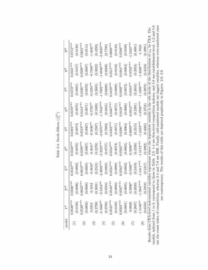
The empirical strategy adopted here is to regress deciles of the CEA-level distribution of observed
ωit on the competition index cm(i)t, instrumented for by the set of demand shifters:
(2.5) ρ(k)mt = β
(k)d cmt + νmt
– where ρ(k) is the kth decile (so that k ∈ 1, . . . , 9) of the distribution of ωit in market m, and the
unit of observation is the market.
The implication of figure 2 from section 6.1.1 is clear: β(k)d should be decreasing in k. The
prediction of the X-inefficiency story is dependent on the parametric assumption of a constant
effect, therefore the main interest is to ask whether the movement of β(k)c in k is consistent with the
truncation shift.
18The argument made by figure 2 is impressionistic, and the figures depict a normal distribution. A more completemodel would require substantial additional assumptions, parametric and otherwise, to capture the dynamic implica-tions of a linear shift or a shift in the truncation point, however the intuition here is clear: mechanisms that workvia shifts affect the entire distribution, while mechanisms that operate on the truncation point will affect primarilythe left tail. An fully specified example of an industry dynamics model which generates these results is offered byCombes, Duranton, Gobillon, Puga, and Roux (2010).
15

2.6.1.3 Results
Though the argument has been somewhat informal, the results offered in Table 2.4 and depicted
graphically in Figures 6-9 are stark. Contrary to the prediction of the dynamic selection story, β(k)d
seems to be constant or increasing in k; sharply increasing at the far right tail.19
The above is not a formal statistical test, but offers strong evidence against the null that dynamic
selection is the primary story. To develop this identification strategy more rigorously would require
extensive assumptions, parametric and otherwise. The next section offers a rigorous, structural
identification strategy without such assumptions and, further, can measure the relative contribution
of both stories to the observed correlation.
2.6.2 The Selection Correction Approach
Reconsider briefly the reduced-form IV regression run in section 3, where the competition index
cm(i)t is instrumented for using the set of demand shifters:
ωit = β1 + βIV cm(i)t + εit
The elasticity coefficient βIV was interpreted as the reduced-form correlation coefficient of pro-
ductivity and competition. However, by imposing additive separability of X-inefficiency and idiosyn-
cratic productivity as well as linearity of the effect of competition20 one can go further:
(2.6) ωit = βXcm(i)t + φit
The coefficient βX is interpreted as a structural primitive describing X-inefficiency, and the
divergence between the true βIV and the correlation coefficient estimated in section 3 stems from
selection biased induced by dynamic selection. The error term, φit, has a structural interpretation
as well, as establishment-level idiosyncratic productivity.
With parametric restrictions, one could proceed with a selection correction in the spirit of Heck-
man (1979). Alternatively, with data on the selection-relevant observables for non-selected firms, a
nonparametric selection-correction would be viable. An aversion to parametric restrictions and a
lack of such data makes the selection problem difficult.
19Because HHI is a measure of concentration rather than competition, both the prediction and the results are ofopposite sign.
20Linearity is assumed for comparison with βIV . The relationship between cm(i)t and ωit is nonparametricallyidentified.
16
A way forward, borrowed from Olley and Pakes (1996), is to give up one year of data and impose
a stricter selection rule: that the firm was observed at time t− 1. If the bias induced can be written
in terms of time t and t − 1 observables, a control function can be used to solve the endogeneity
problem. In the next two sections, just such a control function is derived from a model of the decision
problem of the firm.
2.6.2.1 The Firm’s Decision Problem
In order to capture the bias explicitly, a fuller model of the firm’s exit choice is presented. It is a
finite-firm model with multidimensional states in the spirit of Ericson and Pakes (1995) as extended
by Doraszelski and Satterthwaite (2010).
Stage-game profits are given by R(φit, xit, Sm(i)t, dm(i)t), where φit represents, as before, the
idiosyncratic establishment-level productivity shock, xit is a vector of firm-specific state variables
(e.g., capital, age, and idiosyncratic establishment-level demand), the state of the market Sm(i)t
includes all firms’ types, and dm(i)t is a vector of exogenous demand shifters. The first assumption
is the timing of play:
(A1) φ evolves→ stage game → entry and exit
The conclusions here are robust to entry before exit and vice versa, as well as to the inclusion of
choice variables which affect the firm specific state in xit. What is important about (A1) is that the
stage game is played at the new productivity level and before the exit decision, which implies that
in the data-generating process, observables are generated even for exiting firms. At the time of the
exit choice, the firm is assumed to condition on the following information set:
(A2) Iit ≡< φit, xit, Sm(i)t, dm(i)t >
Firms’ decisions may affect both their owns states and the state of the market. However, φit is
assumed to evolve according to an exogenous Markov process. Formally,
(A3) p(φit|Iit−1) = p(φit|φit−1)
Additional assumptions are required to guarantee existence of equilibrium with a nonempty set
17

of active firms in this market, however that is beyond the scope of this paper. The interested reader
is referred to Doraszelski and Satterthwaite (2010). These assumptions are made for the purposes
of identification, as discussed below, where one can also find a discussion of the implications of
weakening or reversing them.
2.6.2.2 Identification
Recall (2.6), which formally nests the X-inefficiency hypothesis:
ωit = βXcm(i)t + φit
The stricter selection rule allows one to condition both on the information set of the firm at
time t− 1 as well as survival from t− 1. Let φ∗it be the minimum φ required to sustain nonnegative
expected discounted profits; then, survival from t − 1 implies φit−1 ≥ φ∗m(i)t−1. In order to derive
the selection correction in terms of observables, one takes the expectation of both sides of (2.6)
conditional on < Iit−1, φit−1 ≥ φ∗m(i)t−1 >:
E[φit|Iit−1, φit−1 > φ∗m(i)t−1] =β0 + βXE[cm(i)t|Iit−1, φit−1 > φ∗m(i)t−1]
+ E[φit|Iit−1, φit > φ∗m(i)t](2.7)
Focusing on the last term, which represents selection bias, note that (A1) and (A2) imply that
φit−1 > φ∗m(i)t−1 is fully determined by Iit−1. Therefore,
(2.8) E[φit|Iit−1, φit > φ∗m(i)t] = E[φit|Iit−1]
Moreover, the exogeneity of the Markov process (A3) implies that the only relevant information in
Iit−1 for the expected value of φit is φit−1
E[φit|Iit−1] = E[φit|φit−1]
= ψ(φit−1)
– where ψ is some unknown function. Though φit−1 is not directly observable, the model implies
φit−1 = ωit−1 − βXcm(i)t−1. As the arguments of the selection bias can be rewritten in terms of
18

observables, a control function can account for the bias:
ωit = β2 + βXcm(i)t + ψ(ωit−1 − βccm(i)t−1) + εit
The function ψ is estimated by sieve, which allows for flexible parametric form that is increasing in
complexity and nonparametric in the limit (see Chen (2007)). That ψ is treated flexibly is important
because its is unknown without substantial further structure and solving a dynamic programming
problem. Since ψ(·) captures the bias conditional on prior type and survival, the remaining error
εit is mean-zero conditional on Iit−1 by construction. Consistent with (A2), lagged demand shifters
are used to instrument for cm(i)t. Alternatively, one could modify (A2) to give firms foresight, in
which case contemporary instruments would be appropriate.
Given an estimate of βX , one can go a step further to capture the dynamic selection effect by a
reduced-form parameter denoted βDS , which will offer a useful point of comparison. First, net out
βXcm(i)t from ωit to obtain φit. Then run the following regression, instrumenting for cm(i)t using
the set of demand shifters:
(2.9) φit = β3 + βDScm(i)t + ξit
The null of X-inefficiency only implies that βDS = 0. The story captured by βDS is the selection
effect. The limited modeling assumptions imposed by this paper offer no structural interpretation,
however βDS can be thought of as the reduced-form average dynamic selection effect weighted by
the sample of markets observed, which can be compared in magnitude to βX . In this sense, the
model nests both X-inefficiency and dynamic selection as explanations for the correlation found in
the IV regressions of section 3.
Intuitively, identification hinges on being able to write the bias introduced by selection as a
function of objects which are either observed or implied by the model. By controlling for φit−1
nonparametrically, the variation which remains is innovation in productivity. Some of this innovation
may be explained by exogenous shocks to competition as predicted by the set of instruments for
demand, and the rest is explained by the Markov evolution (A3) of productivity types.
19

2.6.2.3 Results
Estimates from the selection correction model are presented in Table 2.5 for each of the eight
specifications presented in the IV and quantile approaches. The first set of results present the
nonlinear two-stage least-squares estimates of βX , the primitive describing the direct effect of X-
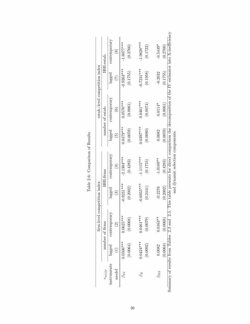
inefficiency. The second set offer a reduced-form estimate of the contribution of the dynamic selection
story, βDS . These results are condensed and presented in comparison with the IV estimates from
section 3 in Table 2.6.
After taking out the direct causal effect, only in models (2) and (4) does one obtain a statistically
significant (at the 0.05 level) βDS . The results suggest that X-inefficiency explains the majority of
the correlation identified by βIV . To ask this question in another way, probits were run to ask how
whether competition, instrumented by the set of demand shifters, predicts survival into the next
period, conditional on type and other observable characteristics of the establishment. Coefficient
estimates are presented in Table 2.7. Confirming intuition, productivity is clearly correlated with
survival; however the insignificance of the coefficient on cm(i)t supports the conclusion that dynamic
selection is not an economically significant story in this industry.21
2.7 Conclusion
This paper has offered evidence for a correlation between competition and productivity in ready-
mix concrete. Two explanations were identified from the literature: X-inefficiency and dynamic
selection, and two empirical strategies were developed and implemented to nonparametrically dis-
tinguish between them. The quantile approach yielded results directly opposite those predicted by
the dynamic selection story: the biggest movements in the distribution of productivity residuals was
in the right tail rather than in the left. The selection correction approach, on the other hand, was
able to measure the relative contribution of the two stories, and weighed in emphatically behind
X-inefficiency.
In some ways this result is unsatisfying; X-inefficiency is the less-specified of the two stories, and
the conclusion here begs the question of what is driving the within-firm response to competition.
Some reflections can be gleaned from the evidence compiled here. For instance, the movement of
the right tail would imply that bankruptcy aversion is not the primary story in ready-mix concrete.
A fuller treatment of this question is beyond the scope of this paper, but an important direction for
21Results in Table 2.7 are coefficients and not marginal effects; the emphasis here is on the insignificance, ratherthan the magnitude of the effect. See Collard-Wexler (2011) for extensive further work on the determinants of selectionin the ready-mix concrete industry.
20

future research. It is only with a theoretical framework to explain the direct productivity response
that one can begin to assess the welfare implications of these productive efficiencies.
Leibenstein (1966) observed that if productivity and competition are correlated, then the Econ
101 story of deadweight loss triangles may not be the most compelling reason to worry about fostering
robust competition. The first step towards turning that observation into policy prescription is to
understand the source of the correlation, a matter on which no consensus has been reached. The
evidence compiled here suggests that the way forward is to look within the firm at the organization
of production.
21
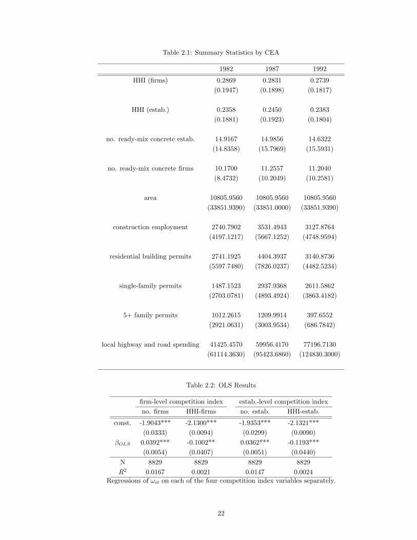
Table 2.1: Summary Statistics by CEA
1982 1987 1992
HHI (firms) 0.2869 0.2831 0.2739
(0.1947) (0.1898) (0.1817)
HHI (estab.) 0.2358 0.2450 0.2383
(0.1881) (0.1923) (0.1804)
no. ready-mix concrete estab. 14.9167 14.9856 14.6322
(14.8358) (15.7969) (15.5931)
no. ready-mix concrete firms 10.1700 11.2557 11.2040
(8.4732) (10.2049) (10.2581)
area 10805.9560 10805.9560 10805.9560
(33851.9390) (33851.0000) (33851.9390)
construction employment 2740.7902 3531.4943 3127.8764
(4197.1217) (5667.1252) (4748.9594)
residential building permits 2741.1925 4404.3937 3140.8736
(5597.7480) (7826.0237) (4482.5234)
single-family permits 1487.1523 2937.9368 2611.5862
(2703.0781) (4893.4924) (3863.4182)
5+ family permits 1012.2615 1209.9914 397.6552
(2921.0631) (3003.9534) (686.7842)
local highway and road spending 41425.4570 59956.4170 77196.7130
(61114.3630) (95423.6860) (124830.3000)
Table 2.2: OLS Results
firm-level competition index estab.-level competition index
no. firms HHI-firms no. estab. HHI-estab.
const. -1.9043*** -2.1300*** -1.9353*** -2.1321***
(0.0333) (0.0094) (0.0299) (0.0090)
βOLS 0.0392*** -0.1002** 0.0362*** -0.1193***
(0.0054) (0.0407) (0.0051) (0.0440)
N 8829 8829 8829 8829
R2 0.0167 0.0021 0.0147 0.0024
Regressions of ωit on each of the four competition index variables separately.
22
Tab
le2.3
:In
stru
men
tal
Vari
ab
les
Res
ult
s
firm
-lev
elco
mp
etit
ion
ind
exes
tab
.-le
vel
com
pet
itio
nin
dex
c m(i
)tnu
mb
erof
firm
sH
HI-
firm
snu
mb
erof
esta
b.
HH
I-es
tab
.
inst
rum
ents
lagg
edco
nte
mp
orar
yla
gged
conte
mp
ora
ryla
gged
conte
mp
ora
ryla
gged
conte
mp
ora
ry
mod
el(1
)(2
)(3
)(4
)(5
)(6
)(7
)(8
)
con
st.
-1.7
837*
**-1
.770
3***
-1.9
261***
-1.7
548***
-1.8
142***
-1.8
191***
-1.9
643***
-1.9
183***
(0.0
398)
(0.0
429)
(0.0
346)
(0.0
776)
(0.0
346)
(0.0
364)
(0.0
229)
(0.0
375)
βIV
0.05
06**
*0.
0625
***
-0.9
231***
-2.1
304***
0.0
479***
0.0
576***
-0.9
263***
-1.6
077***
(0.0
064)
(0.0
068)
(0.2
002)
(0.4
283)
(0.0
059)
(0.0
061)
(0.1
755)
(0.2
760)
N57
7185
215771
8521
5771
8521
5771
8521
firs
t-st
age
F-t
est
188.
0519
9.41
3.0
81.7
0238.9
3245.5
13.7
92.4
8
IVre
gres
sion
sofωit
onco
mp
etit
ion
ind
exva
riab
les
usi
ng
the
foll
owin
gin
stu
men
ts,
eith
erla
gged
or
conte
mp
ora
ry:
gen
eral
con
stru
ctio
nem
plo
ym
ent,
resi
den
tial
bu
ild
ing
per
mit
s,si
ngle
-fam
ily
resi
den
ceb
uil
din
gp
erm
its,
5+
fam
ily
resi
den
cebu
ild
ing
per
mit
s,an
dlo
cal
gov
ern
men
th
ighw
ayex
pen
dit
ure
s,al
lp
ersq
uar
em
ile.
Th
efi
rst-
stage
F-t
est
isfr
om
ase
para
te,
CE
A-l
evel
regre
ssio
nof
the
com
pet
itio
nin
dex
on
inst
rum
ents
.
23
Tab
le2.4
:D
ecil
eE
ffec
ts(β
(k)
d)
mod
el1st
2nd
3rd
4th
5th
6th
7th
8th
9th
(1)
0.05
39**
*0.
0566
***
0.0
543***
0.0
540***
0.0
494***
0.0
478***
0.0473***
0.0
531***
0.0
712***
(0.0
109)
(0.0
096)
(0.0
092)
(0.0
076)
(0.0
074)
(0.0
078)
(0.0
091)
(0.0
107)
(0.0
139)
(2)
0.05
29**
*0.
0622
***
0.0
619***
0.0
589***
0.0
519***
0.0
444***
0.0426***
0.0
509***
0.0
631***
(0.0
092)
(0.0
088)
(0.0
085)
(0.0
067)
(0.0
067)
(0.0
071)
(0.0
076)
(0.0
087)
(0.0
114)
(3)
0.03
53-0
.424
3-0
.4610*
-0.4
641*
-0.5
836**
-0.5
793**
-0.5
291**
-0.7
889**
-1.4
635**
(0.2
799)
(0.2
691)
(0.2
524)
(0.2
376)
(0.2
387)
(0.2
409)
(0.2
685)
(0.3
032)
(0.4
293)
(4)
-2.1
660*
*-2
.345
3**
-2.2
692***
-2.3
225***
-2.0
275***
-1.7
842***
-1.7
392***
-1.8
826***
-2.3
333***
(0.9
798)
(0.9
584)
(0.8
805)
(0.8
757)
(0.7
603)
(0.6
855)
(0.6
680)
(0.6
800)
(0.7
788)
(5)
0.05
25**
*0.
0548
***
0.0
524***
0.0
524***
0.0
482***
0.0
467***
0.0459***
0.0
517***
0.0
698***
(0.0
108)
(0.0
093)
(0.0
088)
(0.0
073)
(0.0
071)
(0.0
075)
(0.0
088)
(0.0
103)
(0.0
133)
(6)
0.05
03**
*0.
0587
***
0.0
583***
0.0
563***
0.0
490***
0.0
416***
0.0409***
0.0
484***
0.0
589***
(0.0
091)
(0.0
085)
(0.0
082)
(0.0
065)
(0.0
064)
(0.0
068)
(0.0
074)
(0.0
084)
(0.0
109)
(7)
-0.0
630
-0.5
096*
-0.5
560**
-0.5
698**
-0.6
689***
-0.6
813***
-0.6
318**
-0.8
702***
-1.5
342***
(0.2
697)
(0.2
620)
(0.2
419)
(0.2
330)
(0.2
315)
(0.2
391)
(0.2
645)
(0.2
924)
(0.4
081)
(8)
-1.5
186*
*-1
.594
7***
-1.5
411***
-1.5
172***
-1.2
423***
-1.0
709***
-1.1
209***
-1.3
330***
-1.7
023
(0.6
550)
(0.5
919)
(0.5
317)
(0.4
992)
(0.4
085)
(0.3
758)
(0.3
978)
(0.4
319)
(0.4
991)
Res
ult
sfr
omC
EA
-lev
elin
stru
men
tal
vari
able
sre
gre
ssio
ns
wh
ere
the
dep
end
ent
vari
ab
leis
then
thd
ecil
eof
the
dis
trib
uti
on
ofωit
by
CE
A.
Th
em
od
els,
ind
exed
from
1to
8,co
rres
pon
dto
thos
ein
Tab
le2.3
:1-4
use
firm
-lev
elco
mp
etit
ion
ind
exes
,an
d5-8
use
esta
bli
shm
ent-
leve
l.1-2
an
d5-6
use
the
cou
nt
ind
exof
com
pet
itio
n,
wh
erea
s3-
4an
d7-8
use
HH
I.F
inall
y,od
d-n
um
ber
edm
od
els
use
lagged
vari
ab
les,
wh
erea
sev
en-n
um
ber
edon
esu
seco
nte
mp
orar
y.T
he
resu
lts
of
this
tab
leare
dep
icte
dgra
ph
icall
yin
Fig
ure
s2.6
-2.9
.
24

Tab
le2.5
:In
stru
men
tal
Vari
able
sw
ith
Sel
ecti
on
Corr
ecti
on
Res
ult
s
firm
-lev
elco
mp
etit
ion
ind
exes
tab
.-le
vel
com
pet
itio
nin
dex
c m(i
)tnu
mb
erof
firm
sH
HI-
firm
snu
mb
erof
esta
b.
HH
I-es
tab
.
inst
rum
ents
lagg
edco
nte
mp
orar
yla
gged
conte
mp
ora
ryla
gged
conte
mp
ora
ryla
gged
conte
mp
ora
ry
mod
el(1
)(2
)(3
)(4
)(5
)(6
)(7
)(8
)
con
st.
-3.2
914*
**-0
.444
8*1.3
591**
-0.1
113
0.5
798
-0.5
795**
0.7
297
0.5
465
(0.3
548)
(0.2
575)
(0.6
670)
(0.3
860)
(0.4
866)
(0.2
478)
(0.5
162)
(0.6
295)
βX
0.04
24**
*0.
0461
***
-0.6
955***
-1.1
115***
0.0
397***
0.0
461***
-0.7
231***
-1.0
628***
(0.0
092)
(0.0
079)
(0.2
441)
(0.1
755)
(0.0
080)
(0.0
074)
(0.1
958)
(0.1
722)
N36
0035
133600
3513
3600
3513
3600
3513
con
st.
-1.7
837*
**-1
.770
3***
-1.9
261***
-1.7
548***
-1.8
142***
-1.8
191***
-1.9
643***
-1.9
183***
(0.0
398)
(0.0
429)
(0.0
346)
(0.0
776)
(0.0
346)
(0.0
364)
(0.0
229)
(0.0
375)
βDS
0.00
820.
0163
**-0
.2276
-1.0
189**
0.0
082
0.0114*
-0.2
032
-0.5
449*
(0.0
064)
(0.0
068)
(0.2
002)
(0.4
283)
(0.0
059)
(0.0
061)
(0.1
755)
(0.2
760)
N57
7185
215771
8521
5771
8521
5771
8521
Th
isp
anel
dep
icts
two
sets
ofre
sult
sfo
rea
chm
od
el.
Th
efi
rst
ob
tainβX
from
the
sele
ctio
nco
rrec
tion
pro
ced
ure
wh
ich
contr
ols
non
para
met
rica
lly
forφit−
1.
Th
ese
con
dse
tof
resu
lts
obta
inβDS
by
an
inst
rum
enta
lva
riab
les
regre
ssio
nof
the
imp
lied
φit
on
com
pet
itio
nin
dex
es.
25
Tab
le2.6
:C
om
pari
son
of
Res
ult
s
firm
-lev
elco
mp
etit
ion
ind
exes
tab
.-le
vel
com
pet
itio
nin
dex
c m(i
)tnu
mb
erof
firm
sH
HI-
firm
snu
mb
erof
esta
b.
HH
I-es
tab
.
inst
rum
ents
lagg
edco
nte
mp
orar
yla
gged
conte
mp
ora
ryla
gged
conte
mp
ora
ryla
gged
conte
mp
ora
ry
mod
el(1
)(2
)(3
)(4
)(5
)(6
)(7
)(8
)
βIV
0.05
06**
*0.
0625
***
-0.9
231***
-2.1
304***
0.0
479***
0.0
576***
-0.9
263***
-1.6
077***
(0.0
064)
(0.0
068)
(0.2
002)
(0.4
283)
(0.0
059)
(0.0
061)
(0.1
755)
(0.2
760)
βX
0.04
24**
*0.
0461
***
-0.6
955***
-1.1
115***
0.0
397***
0.0
461***
-0.7
231***
-1.0
628***
(0.0
092)
(0.0
079)
(0.2
441)
(0.1
755)
(0.0
080)
(0.0
074)
(0.1
958)
(0.1
722)
βDS
0.00
820.
0163
**-0
.2276
-1.0
189**
0.0
082
0.0114*
-0.2
032
-0.5
449*
(0.0
064)
(0.0
068)
(0.2
002)
(0.4
283)
(0.0
059)
(0.0
061)
(0.1
755)
(0.2
760)
Su
mm
ary
ofre
sult
sfr
omT
able
s2.
3an
d2.
5.T
his
tab
lep
rese
nts
for
dir
ect
com
pari
son
the
dec
om
posi
tion
of
the
IVes
tim
ato
rin
toX
-in
effici
ency
an
dd
yn
am
icse
lect
ion
com
pon
ents
.
26

Fig
ure
2.1
:C
ou
nty
Map
of
the
US
A
27

Fig
ure
2.2
:C
EA
Map
of
the
US
A
28
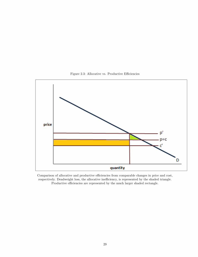
Figure 2.3: Allocative vs. Productive Efficiencies
Comparison of allocative and productive efficiencies from comparable changes in price and cost,respectively. Deadweight loss, the allocative inefficiency, is represented by the shaded triangle.
Productive efficiencies are represented by the much larger shaded rectangle.
29

Figure 2.4: Value Function Response to Change in Market Size.
(a)
(b)
(c)
30
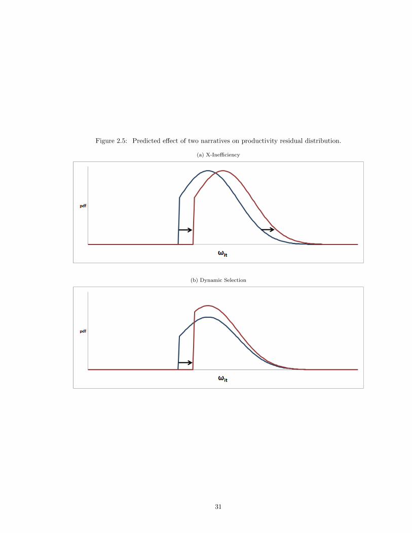
Figure 2.5: Predicted effect of two narratives on productivity residual distribution.
(a) X-Inefficiency
(b) Dynamic Selection
31
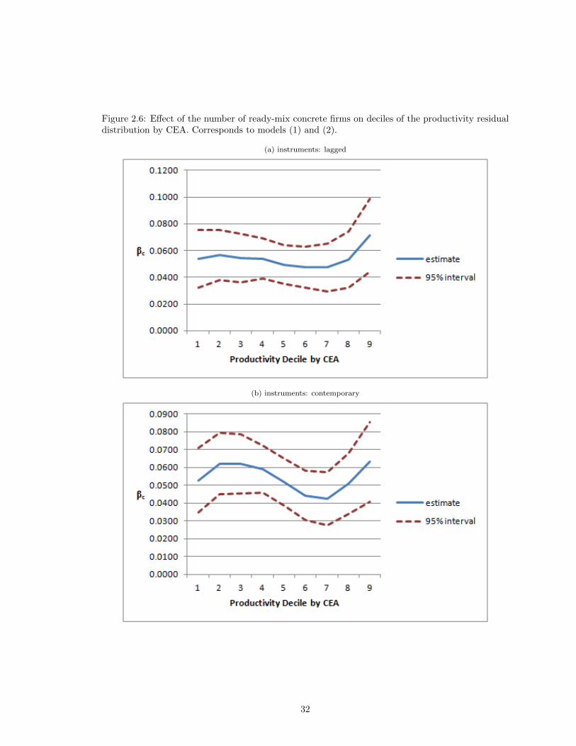
Figure 2.6: Effect of the number of ready-mix concrete firms on deciles of the productivity residualdistribution by CEA. Corresponds to models (1) and (2).
(a) instruments: lagged
(b) instruments: contemporary
32

Figure 2.7: Effect of HHI (calculated using firms) on deciles of the productivity residual distributionby CEA. Corresponds to models (3) and (4).
(a) instruments: lagged
(b) instruments: contemporary
33

Figure 2.8: Effect of the number of ready-mix concrete establishments on deciles of the productivityresidual distribution by CEA. Corresponds to models (5) and (6).
(a) instruments: lagged
(b) instruments: contemporary
34
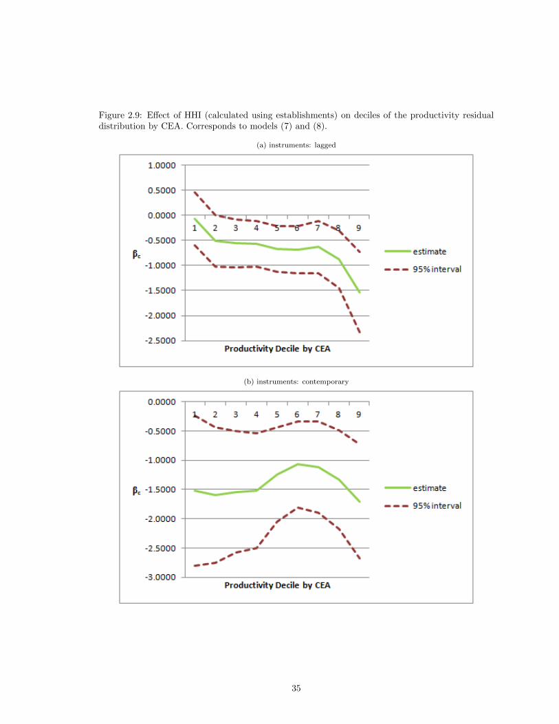
Figure 2.9: Effect of HHI (calculated using establishments) on deciles of the productivity residualdistribution by CEA. Corresponds to models (7) and (8).
(a) instruments: lagged
(b) instruments: contemporary
35

Table 2.7: Probit Results
firm-level competition index estab.-level competition index
no. firms HHI-firms no. estab. HHI-estab.
constant 0.9993*** 0.9900*** 0.9821*** 0.9631***
(0.1910) (0.1740) (0.1858) (0.1640)
cm(i)t 0.0170 -0.5981 0.0143 -0.6321
(0.0197) (0.5460) (0.0190) (0.5238)
ωit 0.3131*** 0.3069*** 0.3151*** 0.3061***
(0.0590) (0.0599) (0.0590) (0.0598)
K (structures) 0.0169 0.0166 0.0165 0.0158
(0.0250) (0.0250) (0.0250) (0.0250)
K (equipment) 0.1179*** 0.1164*** 0.1185*** 0.1182***
(0.0234) (0.0235) (0.0234) (0.0234)
age -0.0219*** -0.0223*** -0.0218*** -0.0220***
(0.0032) (0.0032) (0.0032) (0.0032)
Results from instrumental variables probit regressions of survival dummies (χt = 1 iff the firm ispresent at time t+ 1) on firm observables. The competition index cm(i)t is defined by the model.Capital is observed in two forms in the Census of Manufactures data, structures (e.g., buildings)
and equipment (e.g., ready-mix concrete trucks). Age is constructed from the LBD. Allinstruments are contemporary.
36
CHAPTER III
General Comparative Statics for Industry Dynamics inLong-Run Equilibrium
3.1 Introduction
When claims are made about long-run supply, barriers to entry, or the decision to close down
a plant, some notion of industry dynamics is usually implicit in the motivation. However, the
formalization of that motivation often relies on static, two-stage, or highly parameterized models,
due in large part to the intractability and nonlinearity of dynamic models. This paper builds on
the framework of Hopenhayn (1992a) to show that comparative statics results can be obtained in a
general industry dynamics model from a set of intuitive and economically meaningful assumptions.
The results offer new intuition for why industry groups lobby for strict licensing requirements, both
the transience and high quality of New York restaurants, and why there is little turnover in industries
with high sunk costs.
A surprising and salient feature of micro production data is the persistence of productivity
differences among firms, even in seemingly narrow and homogeneous industries. Matching this
heterogeneity was an important hurdle for the early industry dynamics literature. The critical
innovation which permits of modeling heterogeneity in equilibrium is the introduction of firm-level
idiosyncratic shocks, an idea which traces its roots to Alchian (1950). Lippman and Rumelt (1982)
formalizes Alchian’s argument for luck as “uncertain imitability,” presaging two important features of
the literature to come: free entry by an unlimited pool of ex-ante identical competitors and rational
behavior by participants conditional on their idiosyncratic type. The seminal paper, Hopenhayn
(1992a), extends that model to an infinitely repeated game with Markov idiosyncratic types and
demonstrates the existence of an equilibrium with an ergodic distribution of types that sustains
heterogeneity.
One of the great challenges of this literature is obtaining comparative statics. A change in market
37
fundamentals changes firm payoffs and subsequently entry and exit, which in turn affects the ergodic
distribution of active types. Because the usual objects of interest (e.g., average type) are functionals
of that ergodic distribution, it is inherently difficult to relate them back to market fundamentals.
Though a handful of comparative static results are obtained in Hopenhayn (1992a) and Hopenhayn
(1992b), the assumptions required aree restrictive and the proofs are difficult.
Insofar as Hopenhayn (1992a) found great success as a general modeling framework and limited
power as a predictive engine, Melitz (2003) paved the way for a literature with the opposite strengths.
By imposing strong parametric structure on the problem, this literature was able to obtain closed-
form analytic solutions for a broad set of comparative statics and further, a model with which to
analyze trade liberalization from an industry dynamics perspective.
This paper will vindicate a number of those comparative statics, in particular those with respect
to market size, and demonstrate the generality of the economic logic which underlies them. Section
2 develops the formal model; Section 3 formalizes the idea of competitive stationary equilibrium and
proves existence and uniqueness; Section 4 develops the comparative statics of interest, and Section
5 concludes.
3.2 Model
This section elaborates a model of industry dynamics with heterogeneous firms and endogenous
entry and exit. All firms are endowed with an idiosyncratic type, which can be interpreted as pro-
ductivity or cost advantages that are unique to the firm and not purchased as a factor of production.
Firms pay a fixed cost of entry to learn their initial type and participate in the market. These id-
iosyncratic types evolve over time, and every period firms compete in the marketplace to generate
profits which depend on their type, the types of other competing firms, and exogenous market fun-
damentals. Every period firms also decide whether to exit the market. Combined, these entry and
exit decisions imply an endogenous transition dynamic for the set of active firms’ types. The object
of this model is to show transparently how the steady state of that transition dynamic depends on
the exogenous parameters of profit function and the entry cost.
3.2.1 Idiosyncratic Types
Every firm is endowed with an idiosyncratic type ϕ which is assumed to lie in [0, 1]. Firms are
atomless; at any period t, there is some mass Mt ∈ R+ of firms that are active in the market. Let µt
be a continuous probability density with support [0, 1] which represents the density of active firms’
38

types. Next, let µt ≡Mt · µt; this is the measure of active firms’ types. It captures both the extent
and the character of competition.
Idiosyncratic types are not fixed; every period they evolve as a Markov process according to
F (ϕ′|ϕ). The following assumption is made on that transition rule:
Assumption 1. F (ϕ′|ϕ) is a continuous distribution with following properties:
(a) F has full support on [0, 1] for any ϕ.
(b) F is increasing in ϕ in the sense of first-order stochastic dominance.
The terms “increasing” and “decreasing” are meant weakly in all of what follows unless otherwise
noted. Continuity and full support are technical conveniences, but part (b) carries some economic
intuition. If ϕ is interpreted as productivity, this condition implies serial correlation in idiosyncratic
productivity levels, an stylized fact from the empirical literature on plant-level productivity.
3.2.2 Stage Game
Firms compete to generate profits every period. This model is agnostic about the form of that
competition. Instead, π(ϕ, µ;D) is used to represent the outcome, which is allowed to depend on
firm type ϕ; the measure of competing firms’ types µ, and an exogenous profitability shifter D.
The parameter D is treated as exogenous and fixed, and therefore has no import for considerations
of existence or uniqueness. It is discussed at length in the section on comparative statics. Firms
discount future stage game profits according to a common discount rate β.
Assumption 2. The stage-game profit function π(ϕ, µ;D) is a bounded and continuous function
with the following properties:
(a) π is strictly increasing in ϕ.
(b) π is decreasing in µ with respect to an ordering ≺ that has the following properties:
• ≺ is a complete ordering on the set of bounded continuous functions over the range [0, 1].
• For two distributions µ1 and µ2, with µ2(A) > µ1(A) for some open set A ⊆ [0, 1] and
µ2 ≥ µ1 elsewhere, µ1 ≺ µ2.
(c) For any D, ∃ µ such that ∀ϕ, π(ϕ, µ;D) < 0 as well as a µ′ ≺ µ such that ∀ϕ, π(ϕ, µ′, D) > 0.
Assumption 2 imposes structure on the stage-game profit function. Part (a) is a monotonicity
condition, consistent with the interpretation of type as productivity, costs, or quality. The second
39

restriction (b) imposes a complete order on measures µ. That π is decreasing with respect to a
common ordering ≺ can be interpreted as meaning that firms of all types agree on what constitutes
a more or less competitive market. This rules out most forms of horizontal competition. While ≺
is left mostly unspecified, (b) imposes that adding more competing firms always reduces profits.1
Finally, (c) will be useful for guaranteeing the existence of an interior solution.
Remark
The fact that ≺ is a complete ordering on the set of bounded, continuous functions over [0, 1]
implies that there is a function C(µ) which maps into [0, 1] such that π(ϕ, µ;D) > π(ϕ, µ′;D) ⇒
C(µ) < C(µ′). This function C can be thought of as a theoretical counterpart to competition indexes
such as Herfindal-Hirschman Index and the CRn.
3.2.3 Entry and Exit
There is an unlimited pool of ex-ante identical entrants, who each period choose to either enter
the market or not. Entrants pay a fixed cost cf and learn their initial type ϕ, which is drawn from
F (ϕ|ϕE). The term ϕE is a fixed, exogenous parameter of the model which affects the quality of
new entrants. Let λt denote the endogenous mass of entrants.
The assumption that there is an infinite supply of entrants is important for the comparative
statics and has some bite: for instance, it may be inappropriate to assume that there is an unlimited
pool of firms who could produce high-end computer chips. It may also be implausible in some
markets to assume that, as more and more firms enter, the type of the marginal firm is drawn from
the same distribution as early entrants (i.e., that ϕE does not depend on µt). The importance of
the entry process for proving the results that follow is discussed further in the conclusion.
At the end of each period, firms make an exit choice. Let Xt(ϕ) : [0, 1]→ 0, 1 be the exit rule
at t, with 0 representing exit and 1 representing continued participation in the market2. Exiting
firms receive a payoff normalized to 0.
3.2.4 Timing and Dynamics
The model described above differs somewhat from the literature in the assumption that exit
happens at the end of each period, rather than immediately after entry. To summarize the structure
of each time period:
1This is a standard assumption used by both Hopenhayn (1992a) and Asplund and Nocke (2006).2Xt(ϕ) will be assumed integrable for now, and shown later to take the form of a threshold rule in equilibrium.
40
entry → stage game → exit → types evolve
Intuitively, this is consistent with the idea that firms learn their productivity types by producing
rather than by introspection. This structure has implications for empirical work because the stage
game is the point at which data is generated; see Backus (2011) for more discussion on this point.
The results here are more elegant thanks to, but do not depend on the timing of exit. Note that µt
evolves at several points within each period, therefore it is important to note that by µt this paper
will refer to the measure of types during the stage game.
The timing assumptions above, an entry rate λt+1 and an exit rule Xt(ϕ) together define a law
of motion for µ:
(3.1) µt+1([0, ϕ′]) =
∫ ϕ′
0
∫ 1
0
F (ϕ′|ϕ)Xt(ϕ)dµt(ϕ) + λt+1F (ϕ′|ϕE)
The first term on the right is the measure of incumbents from period t, while the second is
the measure of new entrants at t + 1. Note that despite the introduction of stochastic firm-level
innovations in productivity types, the law of motion for µ is deterministic. This follows from the
decision to model firms as atomless, so that the variance in the realization of their productivity
shocks washes out in the aggregate.
The model specified in this section can be fully characterized by the following set of elements:
π, F,D, cf , ϕE. Given an initial measure µ0 and a strategy profile λt, Xt(ϕ, µt;D), the evolution
of the industry is deterministic. As discussed below in section 3, attention will be restricted to
stationary strategies and a unique ergodic µ, so that the need to specify an initial measure µ0 is
obviated.
3.3 Equilibrium
The value function of the firm may be defined recursively by:
(3.2) vt(ϕ, µt, D) = π(ϕ, µt, D) + max0, β∫vt+1(ϕ′, µt+1, D)dF (ϕ′|ϕ)
Standard dynamic programming arguments demonstrate that firms’ exit strategies can be sum-
marized by a threshold rule, which is denoted by x∗t . All firms with ϕ < x∗t exit the market, and
41

firms of type x∗t are just indifferent:
(3.3)
∫vt(ϕ
′, µt+1, D)dF (ϕ′|x∗t ) = 0
There is also an unlimited pool of potential entrants who have the option to pay a fixed cost cf
to enter and draw iid types from F (ϕ|ϕE). Each period, a mass of firms λt ≥ 0 enter such that
either λt = 0 or the expected value of entry is zero:
(3.4)
∫vt(ϕ, µt, D)dF (ϕ|ϕE)− cf = 0
Given λt+1 and x∗t , the law of motion (3.1) can be simplified:
(3.1’) µt+1([0, ϕ′]) =
∫ 1
x∗t
F (ϕ′|ϕ)dµt(ϕ) + λt+1F (ϕ′|ϕE)
The first integral in (3.1’) is comprised of firms with ϕ > x∗ in period t and the latter, a mass
λt+1 of entrants. Recall that while firms face uncertainty via innovations in idiosyncratic type,
they are atomless and there are no industry-level shocks; therefore dynamics in the aggregate are
deterministic.
Attention is restricted to equilibria in stationary strategies, which will imply an ergodic distri-
bution; a fixed point of 3.1’. In this sense the solution concept characterizes industry dynamics
in long-run equilibrium, and for this reason time subscripts will henceforth be dropped. Moreover,
define:
(3.5) Ψ(ϕ) ≡∫v(ϕ′, µ;D)dF (ϕ′|ϕ)
Intuitively, Ψ(ϕ) is the continuation value of a firm of type ϕ today. βΨ(ϕ) is the relevant
expected payoff for firms deciding whether to exit the market; similarly, Ψ(ϕE) is the expected
payoff to entry. These expressions are useful for characterizing the equilibrium conditions.
A stationary competitive equilibrium of this game is a triple < µ, x∗, λ > such that:
42

1. The measure of active types is self-generating in the sense of (3.1’), so that:
(E1) µ([0, ϕ′]) =
∫ 1
x∗F (ϕ′|ϕ)dµ(ϕ) + λF (ϕ′|ϕE)
2. The marginal incumbent is indifferent:
(E2) Ψ(x∗) = 0
3. The expected value of entry is zero:
(E3) Ψ(ϕE) = cf
The first condition implies stationarity in a strong sense, which obtains from the absence of
market-level shocks. The second implies an optimal exit rule: firms exit if their expected profits are
negative. Finally, the third equilibrium condition requires that the per-period mass of entrants λ is
sufficient to guarantee zero expected profits on entry.
Proposition 1. Under Assumptions 1 - 2: For cf not too large, there exists a at least one equilibrium
with λ > 0.
Proof. See Appendix.
It is a testament to the creativity of that original paper that the proof extends to the imperfectly
competitive case. This is true because it does not rely at all on the perfectly competitive structure or
the price mechanisms in that model. In all of what follows, attention is restricted to the equilibrium
with λ > 0.
Proposition 2. Under Assumptions 1 - 2: The equilibrium of the above game is unique.
Proof of Proposition 2: Suppose by way of contradiction, that there are two distinct equilibria
< µ1, x∗1, λ1 > and < µ2, x
∗2, λ2 >. Suppose µ1 ∼ µ2. Then E2 implies x∗1 = x∗2, which implies
λ1 = λ2. Suppose instead and without loss of generality µ1 ≺ µ2. Then E2 implies x∗1 < x∗2.
However, this yields Ψ1(ϕE) > Ψ2(ϕE), which contradicts E3.
The proof here is rather different from that in Hopenhayn (1992a). In place of assumptions
on factor market prices or the production function, this paper follows Asplund and Nocke (2006)
in taking the more general approach of imposing a complete and common order on the space of
measures µ.
43
3.4 Comparative Statics
The practice of obtaining comparative statics from industry dynamics models is difficult because
the objects of interest are typically functionals of µ, the measure of active types in a stationary
competitive equilibrium. This depends in a non-transparent way on the fundamentals which affect
the rules of transition. In a general setting, it is not possible to obtain explicit solutions.
It is a bit counter-intuitive to talk of comparative statics in an industry dynamics model. The
thought experiment is not a shock to exogenous parameters; no impulse response functions are de-
rived here. Instead, the comparison is between two equilibria, each at their long-run stationary
state. Introducing market-level shocks would require additional assumptions on firms’ beliefs about
the evolution of idiosyncratic types. Simulating them would require significant parametric structure
on the evolution of those shocks and firm profits. Moving in this direction would obviate the primary
advantage of working with a continuum of firms; the ability to do analysis with general functions
because uncertainty washes out in the aggregate. The competing industry dynamics literature fol-
lowing Ericson and Pakes (1995), which works in a discrete environment that lends it to computation
and simulation, is well-suited to modeling short-run dynamics and market-level shocks.
Two comparative statics are derived here for two different exogenous variables. The two outcome
variables of interest are turnover and average type, and the two exogenous variables are fixed costs
of entry and market size. Formally, define the following measure of turnover:
(3.6) T ≡ λ∫µ(ϕ)dϕ
This index is meant to represent the rate of churning in the industry; it is the size of the entering
cohort (equal, by stationarity, to the size of the exiting cohort) relative to the mass of firms in the
industry. Next, define:
(3.7) ϕ ≡∫ϕµ(ϕ)dϕ∫µ(ϕ)dϕ
This term represents the average type in the market. No prior work has been done establishing
results for average type in the general industry dynamics framework. Existing results for average
type stem from the parametric literature following Melitz (2003), e.g., Melitz and Ottaviano (2008),
which address the question of whether average productivity responds to market size and extend that
44

logic to trade liberalization.
Deriving comparative statics for functionals of µ is made tractable by a convenient decomposition
of the ergodic measure proposed by Hopenhayn (1992a). Let µt be a measure over firm types that
have survived into their tth period of existence (e.g., µ1(ϕ) = f(ϕ|ϕE)). Formally, the series of
expressions µt(ϕ)t=1,... is written in terms of x∗ and primitives of the model:
µ1(ϕ) = f(ϕ|ϕE)
µ2(ϕ) =
∫ 1
x∗f(ϕ|ϕ1)f(ϕ1|ϕE)dϕ1
µk(ϕ) =
∫ 1
x∗· · ·∫ 1
x∗f(ϕ|ϕk−1)f(ϕk−1|ϕk−2) · · · f(ϕ2|ϕ1)f(ϕ1|ϕE)d(ϕk−1) · · · dϕ1
The terms µt(ϕ) are measures with the following convenient property: they integrate to the proba-
bility of surviving t periods upon entry. Moreover, they comprise a decomposition of µ:
(3.8) µ = λ
∞∑k=1
µk
In equilibrium µ is completely determined by λ and x∗. This decomposition affords, in principle,
the opportunity to take derivatives of µ with respect to both of these objects.
3.4.1 Fixed Costs of Entry
A staple of the industry dynamics literature is to ask how fixed costs of entry affect market
outcomes. Under a somewhat stronger set of assumptions than those made here, Hopenhayn (1992a)
shows that x∗ is decreasing in cf .3 Propositions 3 and 4 should be thought of as generalizations of
that result to a weaker set of assumptions and a formalization of the implications for turnover and
average type.
Fixed costs of entry cf are incarnated in the real world as irrecoverable investments, such as
highly specific or immobile capital, franchising fees, or licensing fees. Industry groups have been a
powerful force in erecting barriers to entry, especially in the form of licensing fees. While this might
seem counterintuitive at first glance, Figure 3.2 offers some intuition: raising the fixed costs of entry
reduces pressure from entrants, weakening the distribution of competing firms’ types and increasing
3The assumption required is that the profit function is multiplicatively separable into two pars: a function of firms’idiosyncratic types, and a function of market aggregates. This assumption implies, but is not implied by, the existenceof a complete ordering ≺ from Assumption 2 above.
45

profits. The entire continuation value function Ψ(ϕ) shifts up with (ϕE , cf ); it is apparent that
incumbents are beneficiaries of the change.
Proposition 3. Under Assumptions 1 - 2: At the stationary competitive equilibrium, T is decreasing
in cf .
Proof. Lemma 8 of the Appendix demonstrates that T can be written as an increasing function of
x∗. Lemma 6 closes the argument by showing that x∗ is increasing in cf .
The measure of turnover T is normalized with respect to the size of the industry, so it is strictly
increasing in x∗, which determines the likelihood of exit F (x∗|ϕ) for a firm of type ϕ. That exit
threshold x∗ decreases as the entire curve Ψ(ϕ) shifts up; see Figure 3.2.
Proposition 4. Under Assumptions 1 - 2: At the stationary competitive equilibrium, ϕ is decreasing
in cf .
Proof. Lemma 9 of the Appendix demonstrates that ϕ can be written as an increasing function of
x∗. Lemma 6 closes the argument by showing that x∗ is increasing in cf .
As above, the intuition is that x∗ is decreasing because the entire curve Ψ(ϕ) is shifting up;
see Figure 3.2. Getting from there to a decrease in ϕ takes more work; the intuition is that more
low-type firms are sticking around and replacing entrants. Because those entrants have a higher
type on average than the marginal incumbent (see Lemma 3), this lowers average type.
3.4.2 Market Size
Market size in this model is represented by D, which enters the profit function directly. It is
important for the sake of generality to impose minimal parametric form on the way thatD affects firm
profits. Note that while D is construed here as market size, this is merely meant as an interpretive
justification for the set of assumptions which are imposed on the way it enters π. In general, D is a
profitability shifter, and could be used to analyze other exogenous changes, as for instance a change
in corporate tax rates.
Comparative statics with respect to market size are of central importance in recent applications
of industry dynamics because their logic underlies the argument for productivity gains from trade,
e.g. Melitz and Ottaviano (2008). Moreover, they are hard to obtain because the effect of market size
is prima fascia ambiguous. The direct effect of greater market size is to make firms of all types better
off; this should sustain low-type firms, lower x∗, and decrease average productivity and turnover.
46
Entry is the countervailing force. As market size makes all firms better off, more firms enter the
market, reducing profits. Without further structure, parametric or otherwise, it is impossible to sign
the effect.
Two additional assumptions are introduced to obtain comparative statics in D:
Assumption 3 (Competition Reallocates Profits). The stage-game profit function π(ϕ, µ;D) has
increasing differences in ϕ and µ.
This assumption means that competition tends to reallocate profits from low-type to high-type
firms. In this spirit Boone (2008) argues that relative profits between high- and low-type firms is in
fact a direct measure of competition, superior to conventional techniques such as HHI or the number
of firms.
Assumption 4. π(ϕ, µ;D) is continuous and strictly increasing in D and has increasing differences
in ϕ and D.
This assumption means that high-type firms benefit more from an increase in D than low-type
firms. It can be thought of as a restriction on the sorts of profitability shifters under consideration.
Under many models of competition, this is a reasonable property to impose on demand shifters.4
Both of the comparative statics expounded below are corollaries of the core result, stated and
proven as Lemma 7 of the Appendix, that x∗ is increasing in D. This non-obvious result implies that
an increase in D makes low-type firms relatively worse off, despite its direct and positive impact on
profits. The mechanism is that higher profits induce entry, which dominates the direct profit effect
on account of Assumptions 3 and 4, allowing one to sign the ambiguity discussed above. See Figure
3.3 for an illustration: at both levels of D the continuation value function must intersect (ϕE , cf );
the assumptions made imply that for larger markets, the function rotates counter-clockwise, raising
x∗.
This is an excellent example, in the spirit of Vives (2009), of a case where the monotone com-
parative statics properties of the stage game profit function do not carry over to the value function.
It is somewhat redemptive, therefore, that those properties are so critical in the argument for the
comparative statics.
4For intuition, consider Cournot competition between two firms with differing costs. Supposing an inverse demandfunction of the form p(Q) = A− bQ, the firms’ equilibrium profit function is
πi =1
9b(A+ cj − 2ci)
2
Here, increasing differences in A (standing in for D) and −ci (standing in for ϕ) is proven by the positive cross-partial:
∂2πi
∂A∂(−ci)=
4
9b
47

Proposition 5. Under Assumptions 1 - 4: At the stationary competitive equilibrium, T is increasing
in D.
Proof. Lemma 8 of the Appendix demonstrates that T can be written as an increasing function of
x∗. Lemma 7 closes the argument by showing that x∗ is increasing in D.
This proposition follows easily once it is shown that x∗ is increasing in D. Intuitively, a higher
cutoff threshold implies a higher fraction of active firms exiting the market. The result is likely to
resound with those familiar with the transience of New York restaurants.
Proposition 6. Under Assumptions 1 - 4: At the stationary competitive equilibrium, ϕ is nonde-
creasing in D.
Proof. Lemma 9 of the Appendix demonstrates that ϕ can be written as an increasing function of
x∗. Lemma 7 closes the argument by showing that x∗ is increasing in D.
That ϕ increases with x∗ is somewhat less transparent, because more turnover means relatively
more draws from F (ϕ|ϕE), which does not obviously improve productivity. This is addressed by
Lemma 3 of the appendix, which shows that x∗ is always lower than ϕE , so that new entrants always
dominate firms on the margin of exit in type. This result is likely to resound with those familiar
with the quality of New York restaurants.
3.5 Conclusion
Industry dynamics models are enjoying more attention than ever, thanks to the success of the
international trade literature in applying parametric variations to match empirical stylized facts
and bolster the argument for gains from trade. This paper vindicates a number of those results by
demonstrating that the economic logic of the argument does not depend on CES utility functions
or monopolistic competition, but instead a basic economic assumption that increases in market
competitiveness reallocate profits from less to more productive firms.
There are still a number of important assumptions of the Hopenhayn (1992a) framework to
weaken. All of the proofs in this paper take advantage of the construction of idiosyncratic firm type
as being one-dimensional. This has the very convenient implication that for the unique equilibria
of any two distinct parameterizations of the model, there is an explicit ranking by x∗. Therefore
the set of survivors in one equilibrium is always either a strict subset or a strict superset of those in
another equilibrium. This would not be true if the threshold rule were a frontier in multidimensional
48

space. It is easy to imagine that a change in the exogenous parameters could generate a survival rule
which is weaker on one dimension but stronger on another, which would make proving comparative
statics very difficult. The construction of entry - in particular that there is an infinite pool of ex-ante
identical entrants - is also restrictive. It is not difficult to imagine industries, especially high-tech
industries, where this would not be true. Moreover, it is easy to reverse some of the results with
alternative entry models. For instance, if there is a fixed distribution of entrants who know their type
prior to entry, then larger market size would simply induce entry by lower-type firms, decreasing
average type.
These limitations aside, the results here demonstrate that there is a common economic logic
underlying the parameterizations of industry dynamics models that have been used to such great
success in understanding plant-level data by IO and trade economists. The contribution of this
paper is to make that logic explicit in the hope and expectation that it will yield still more testable
predictions in a wider set of markets and environments.
3.6 Appendix
Lemma 1. For F (ϕ′|ϕ) on [0, 1] stochastically increasing in ϕ: if γ(ϕ,D) has increasing differences
in D and ϕ, so too does Γ(ϕ,D) ≡∫ 1
0γ(ϕ′, D)dF (ϕ′|ϕ).
Proof: This is a special case of Theorem 2 from Athey (2000). For an intuitive proof, consider the
following: Without loss of generality, let D1 < D2. It suffices to show that the following expression
is nondecreasing:
Γ(ϕ,D2)− Γ(ϕ,D1) =
∫ 1
0
[γ(ϕ′, D1)− γ(ϕ′, D2)] dF (ϕ′|ϕ)
Note that the expression in brackets is nondecreasing because v(ϕ,D) has increasing differences in
D and ϕ. Therefore, recalling that F (ϕ′|ϕ) is stochastically nondecreasing in ϕ, it must be that the
expectation of the difference is increasing in ϕ.
Lemma 2. Under Assumptions 1 - 2: The value function v(ϕ, µ,D) is strictly increasing in D and
ϕ, and strictly decreasing in µ.
Proof: That v is strictly increasing in D and ϕ, and decreasing in µ follows from standard results,
see SLP. That v is strictly decreasing in µ is implied by the full support condition of Assumption
1: π(ϕ, µ;D) is strictly decreasing in µ for some open set in [0, 1], and that set is in the support of
F (ϕ′|ϕ) for any ϕ.
49
Lemma 3. Under Assumptions 1 - 2: In any equilibrium with nonzero entry, x∗ < ϕE.
Proof. Combining equilibrium conditions 2 and 3, we have:
∫v(ϕ′, µ,D)dF (ϕ′|ϕE) = cf
>
∫v(ϕ′, µ,D)dF (ϕ′|x∗)
Because v is increasing in its first argument by Lemma 2 and F (ϕ′|ϕ) is stochastically increasing in
ϕ, it must be that ϕE > ϕ∗.
Lemma 4. Under Assumptions 1 - 2: For two equilibria with D1 < D2, then µ1 µ2.
Proof: Suppose by way of contradiction that µ2 ≺ µ1. Then,
0 =
∫v(ϕ, µ1, D1)dF (ϕ|ϕE)− cf
<
∫v(ϕ, µ2, D2)dF (ϕ|ϕE)− cf
= 0
The first and last equalities are based on equilibrium condition 3, the entry condition. The middle
inequality follows from D1 < D2, µ1 µ2, and Lemma 2. Combined, they imply a contradiction.
Lemma 5. Under Assumptions 1 - 2: Let π(ϕ,D) ≡ π(ϕ, µ(D), D), where µ(D) is the unique
equilibrium µ associated with D. Then π(ϕ,D) has increasing differences in ϕ and D.
Proof: Existence and uniqueness follow from Proposition 1. Complementarity of µ and D follows
from Lemma 4, so that Assumptions 3 and 4 implies increasing differences for π(ϕ,D).
Lemma 6. Under Assumptions 1 - 2: For two equilibria with cf1 < cf2 , it must be that x∗1 ≥ x∗2.
Proof: From the entry condition:
∫v(ϕ, µ1;D)dF (ϕ|ϕE)− cf2 < 0
Therefore µ1 ≺ µ2. Then from the exit condition:
∫v(ϕ, µ2;D)dF (ϕ|x∗1) ≥ 0
50

So that x∗2 ≤ x∗1, strictly if the above inequality is strict.
Lemma 7. Under Assumptions 1 - 4: For two equilibria with D1 < D2, it must be that x∗1 ≤ x∗2.
Proof: Suppose by way of contradiction that x∗2 < x∗1.
First, consider the following distortion of the value function mapping:5
S(z(ϕ,Di)) ≡
π(ϕ,D) + β
∫z(ϕ′, D)dF (ϕ′|ϕ) if ϕ ≥ x∗
π(ϕ,D) + β∫z(ϕ′, D)dF (ϕ′|x∗) else
Using Blackwell’s Sufficient Conditions it is straightforward to confirm that this is a contraction
mapping. Iterating Sn as n→∞, the contraction converges to v(ϕ,D) by the optimality of x∗: the
contraction mapping has a unique fixed point, and it is easy to check that S(v(ϕ,D)) = v(ϕ,D).
Any property that is preserved both by limits and the contraction mapping S must be true of
v(ϕ,D). Three important properties of v(ϕ,D) can be established on this basis:6
1. Monotonicity of v(ϕ,D) in ϕ: it is easy to see that if z(ϕ,D) is monotone increasing in ϕ, so
too is S(z(ϕ,D)).
2. Continuity of v(ϕ,D) in ϕ: This follows from continuity of π in ϕ. One might worry about
a jump discontinuity at x∗, but the normalization of the exit value guarantees continuity at
that point.
3. Increasing Differences: Let z be chosen from the set of functions satisfying monotonicity and
continuity as above. If z(ϕ,D) has increasing differences, then so too does S(z(ϕ,D)). To see
this, posit z(ϕ,D) with increasing differences. In a slight abuse of notation, let Tz(ϕ,D) be the
function S(z(ϕ,D)) evaluated at (ϕ,D). It remains to show that for ϕ1 ≤ ϕ2 and D1 ≤ D2,
(ID) Sz(ϕ2, D1)− Sz(ϕ1, D1) ≤ Sz(ϕ2, D2)− Sz(ϕ1, D2; )
The proof proceeds by dividing [0, 1] into three regions and showing that the above property
holds for any (ϕ1, ϕ2) drawn from the same region. It is closed by using continuity at the edges
of these regions to extend this argument to (ϕ1, ϕ2) pairs drawn from separate regions.
5The sense in which this is a distortion is that the payoff to exit is normalized to β∫z(ϕ′, D)dF (ϕ′|x∗), where x∗
is the true exit threshold at D. At the correct value function this term goes to zero, by equilibrium condition 2. Thereason this distortion is introduced is to generate continuity for any arbitrary z, which is explored below.
6Note that these properties are proven under the assumption, made by way of contradiction, that x∗2 < x∗1. Theseproperties are proven only for the sake of demonstrating a contradiction, and may not all hold at the true equilibrium.
51

(a) In the region [0, x∗2) :
Sz(ϕ,Di) = π(ϕ,Di) + β
∫z(ϕ′, Di)dF (ϕ′|x∗i )
ID holds by Lemma 5.
(b) In the region [x∗2, x∗1) :
Sz(ϕ,Di) =
π(ϕ,D1) + β
∫z(ϕ′, D1)dF (ϕ′|x∗1) for i = 1
π(ϕ,D2) + β∫z(ϕ′, D2)dF (ϕ′|ϕ) for i = 2
Therefore ID holds from ID of π in ϕ and D as well as the monotonicity of z.
(c) In the region [x∗1, 1] :
Sz(ϕ,Di) = π(ϕ,Di) + β
∫z(ϕ′, Di)dF (ϕ′|ϕ)
Using Lemmas 1 and 5, this is simply the sum of two functions with ID in ϕ and D, and
therefore ID holds for Sz.
Finally, consider (ϕ1, ϕ2) drawn from different regions. The concern here is that there may
be discontinuities, either in Sz(ϕ,D1) at x∗1 or in Sz(ϕ,D2) at x∗2. This is alleviated by the
normalization of the continuation value for β∫z(ϕ′, D)dF (ϕ′|x∗), so that limϕ→x∗ Sz(ϕ,D) =
Sz(x∗, D). Then ID across regions is implied by ID within. For intuition, consider x∗2 < ϕ1 <
x∗1 < ϕ2. ID requries:
Sz(ϕ2, D1)− Sz(x∗1, D1) + Sz(x∗1, D1)− Sz(ϕ1, D1)
≤ Sz(ϕ2, D2)− Sz(x∗1, D2) + Sz(x∗1, D2)− Sz(ϕ1, D2)
Continuity of Sz(ϕ,D) at x∗ implies that (a) is extended to [0, x∗2] and (b) is extended to
[x∗2, x∗1], so that ID here can be obtained by comparing the first two terms and the second two
terms on either side of the inequality independently. ID for these pairs implies ID of the sum.
Recall that E3 requires that Ψ1(ϕ) and Ψ2(ϕ) cross at (ϕE , cf ). However, Lemma 1 combined
with ID of v implies Ψi(ϕ) =∫
has increasing differences in ϕ and D. If x2 < x1, then Ψ(x∗1, D2) >
52
0 = Ψ(x∗1, D1), and increasing differences implies that the two functions never cross, generating a
contradiction.
Lemma 8. Under Assumptions 1 - 2: T is increasing in x∗.
Proof: Employing the decomposition of µ from equation (3.8):
T =λ∫
µ(ϕ)dϕ
=1∫ ∑∞
k=1 µk(ϕ)dϕ
Fixing t,∫µt(ϕ)dϕ corresponds to the probability of surviving t periods conditional on entry, which
is trivially decreasing in x∗ (strictly for t ≥ 2).
Lemma 9. Under Assumptions 1 - 2: ϕ is increasing in x∗.
Proof: Using (3.8), ϕ can be rewritten:
(3.9) ϕ =
∫ϕ∑∞k=1 µk(ϕ)dϕ∫ ∑∞k=1 µk(ϕ)dϕ
Now,
(3.10)
∂ϕ
∂x∗=
∫ϕ∑∞k=1
∂∂x∗ µk(ϕ)dϕ ·
∫ ∑∞k=1 µk(ϕ)dϕ−
∫ ∑∞k=1
∂∂x∗ µk(ϕ)dϕ ·
∫ϕ∑∞k=1 µk(ϕ)dϕ
(∫
∂∂x∗
∑∞k=1 µk(ϕ)dϕ)2
The denominator in (3.10) is trivially positive. In order to sign the numerator, one requires an
expression for the derivative of the sum over µk. To begin,
∂
∂x∗µk(ϕ) = −f(ϕ|x∗)
∫ 1
x∗· · ·∫ 1
x∗f(x∗|ϕk−2) · · · f(ϕ2|ϕ1)f(ϕ1|ϕE)dϕk−2 · · · dϕ1
+
∫ 1
x∗f(ϕ|ϕk−1)
∂
∂x∗
∫ 1
x∗· · ·∫ ∞x∗
f(ϕk−1|ϕk−2) · · · f(ϕ2|ϕ1)f(ϕ1|ϕE)dϕk−1 · · · dϕ1
= −f(ϕ|x∗)µk−1(x∗) +
∫ 1
x∗f(ϕ|ϕk−1)
∂
∂x∗µk−1(ϕk−1)dϕk−1(3.11)
Summing over (3.11) and reorganizing yields:
53

∞∑k=1
∂
∂x∗µk(ϕ) = −f(ϕ|x∗)
∞∑k=2
µk−1(x∗) +
∞∑k=2
∫ 1
x∗f(ϕ|ϕk−1)
∂
∂x∗µk−1(ϕk−1)dϕk−1
= −f(ϕ|x∗)∞∑k=1
µk(x∗) +
∫ 1
x∗f(ϕ|z) ∂
∂x∗
∞∑k=1
µk(z)dz(3.12)
Next, substitute in the left-hand side to solve the expression recursively.
(3.13)
∞∑k=1
∂
∂x∗µk(ϕ) = −
∞∑k=1
µk(x∗)
[f(ϕ|x∗) +
∫ 1
x∗f(ϕ|z1)f(z1|x∗)dz1 + . . .
]
Define ξ(ϕ) ≡∑∞k=1 ξk(ϕ) and ξk(ϕ) ≡
∫ 1
x∗· · ·∫ 1
x∗f(ϕ|zk−1) · · · f(z2|z1)f(z1|x∗)dzk−1 · · · dz1
with ξ1(ϕ) = f(ϕ|x∗). Intuitively, ξk is the distribution of types for a firm that is observed k
periods after having type x∗. This notation affords the following simplification:
∞∑k=1
∂
∂x∗µk(ϕ) = −
∞∑k=1
µk(x∗)
∞∑k=1
ξk(ϕ)
= −∞∑k=1
µk(x∗)ξ(ϕ)(3.14)
Using (3.14) one can revisit the numerator in (3.10):
∫ϕ
∞∑k=1
∂
∂x∗µk(ϕ)dϕ ·
∫ ∞∑k=1
µk(ϕ)dϕ−∫ ∞∑
k=1
∂
∂x∗µk(ϕ)dϕ ·
∫ϕ
∞∑k=1
µk(ϕ)dϕ
=
∫ϕ
( ∞∑k=1
∂
∂x∗µk(ϕ)
∫ ∞∑k=1
µk(ζ)dζ −∞∑k=1
µk(ϕ)
∫ ∞∑k=1
∂
∂x∗µk(ζ)dζ
)dϕ
=
∫ϕ
(−∞∑k=1
µk(x∗)ξ(ϕ)
∫ ∞∑k=1
µk(ζ)dζ +
∞∑k=1
µk(ϕ)
∞∑k=1
µk(x∗)
∫ξ(ζ)dζ
)dϕ
=
[ ∞∑k=1
µk(x∗)
∫ ∞∑k=1
µk(ζ)dζ
∫ξ(ζ)dζ
]∫ϕ
( ∑∞k=1 µk(ϕ)∫ ∑∞k=1 µk(ζ)dζ
− ξ(ϕ)∫ξ(ζ)dζ
)dϕ(3.15)
The term in brackets is trivially positive. The difference integrated in the second term is positive
because the first distribution first-order stochastically dominates the second, as implied by Lemma
3.
54
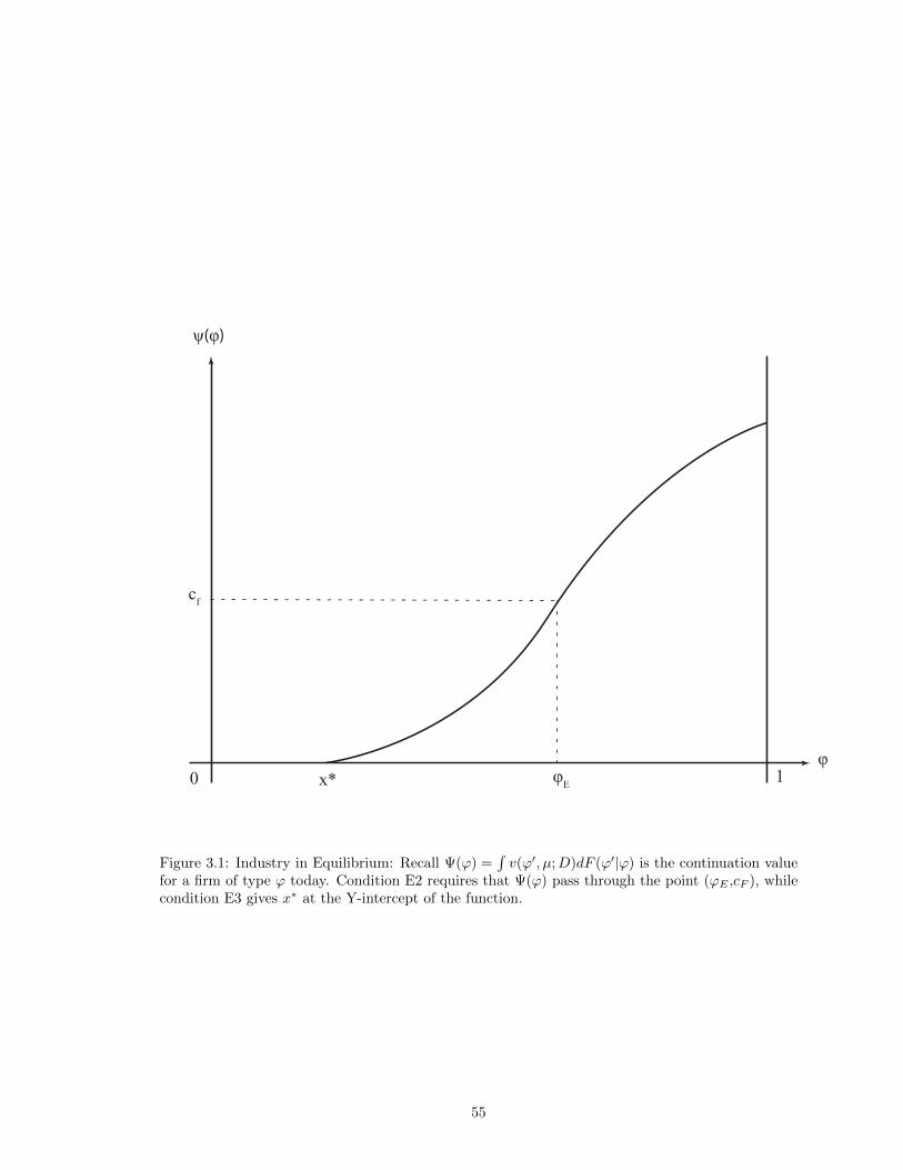
0 1
y(f)
cf
fE
fx*
Figure 3.1: Industry in Equilibrium: Recall Ψ(ϕ) =∫v(ϕ′, µ;D)dF (ϕ′|ϕ) is the continuation value
for a firm of type ϕ today. Condition E2 requires that Ψ(ϕ) pass through the point (ϕE ,cF ), whilecondition E3 gives x∗ at the Y-intercept of the function.
55

0 1
y(f)
cf1
fE
fx1*
cf2
x2*
y1(f)
y2(f)
Figure 3.2: Decrease in Entry Costs: Let cf1 > cf2 . The reduction spurs entry, which drives profitsdown for all types. The new continuation value function Ψ2(ϕ) is smaller than Ψ1(ϕ), and valuedcf2 at ϕE . The exit threshold x∗ rises, spurring higher turnover and average type.
56

0 1
y(f)
cf
fE
fx1* x2*
y1(f)
y2(f)
Figure 3.3: Increase in Market Size: Let D1 < D2. The increase in demand raises profits, inparticular for higher types. The higher profits spur entry, in turn reducing profits, especially forlower types. Combined, these countervailing effects push Ψ2(ϕ) counterclockwise around the originalΨ1(ϕ), pivoting around (ϕE , cf ).
57
CHAPTER IV
An Estimable Demand System for a Large Auction PlatformMarket (with Gregory Lewis)
4.1 Introduction
Most goods and services are sold at fixed prices. Yet auctions are used as the allocation mech-
anism in a wide variety of contexts, including procurement and the granting of oil drilling and
spectrum rights. Online auction platforms, in particular, have grown substantially in recent years.
In retail eBay alone has revenues of $36 billion from its auctions business in 20071, while Google
realized $21 billion in revenue from its online advertising platform in 20082. More specialized auction
sites such as DoveBid and IronPlanet have sold billions of dollars of used aviation and construction
equipment respectively.
Given their importance in the modern economy, one would like to be able to estimate demand in
these platform markets. This would allow us to answer questions of broad economic interest, such
as how much welfare has been generated by these platforms; as well as narrower strategic questions,
such as how a firm with a fixed inventory should set reserves and time sales to dynamically maximize
its revenue. Demand estimation is often also a necessary first step for the evaluation of anti-trust
issues, such as the potential impact on the search-keyword advertising market of a merger between
Microsoft and Yahoo.
At first glance, auctions data is an extremely rich of information about demand. In auctions we
actually observe a continuous bid which directly reflects willingness to pay, relative to the discrete
choice we typically see in fixed price markets. Moreover, for any buyer we generally observe all the
auctions that they bid in, which provides valuable information about which items they view as close
substitutes. This is informative for demand, much in the same way that “second-choice” data is
useful in Berry, Levinsohn, and Pakes (2004). As the choice sets available to buyers vary we may
1Source: eBay Annual Report for 20072Source: Google Annual Report for 2008
58

observe differing participation, which is helpful for identifying substitution patterns.
Yet the strengths of auction market data also pose some difficulties. As Hendricks and Porter
(2007) note in their survey article, participants in auction markets are playing a complex dynamic
game, where they must continuously adapt to the changing set of available auctions, and learn about
rival’s valuations. Most of the existing tools of structural auction econometrics are focused on inde-
pendent auctions of homogenous objects, which limits their direct applicability to auction demand
estimation, where bidders repeatedly interact across auctions, and substitution across products is
important.
In this paper, we develop an estimable demand system for an auction platform market with a
large number of relatively short-lived, yet persistent, buyers. The first part of the paper outlines an
intuitive and empirically tractable equilibrium concept — competitive Markov equilibrium — and
characterizes the long-run distribution of bidders and their strategies. Next, we show that demand
is non-parametrically identified from panel data. In the last part, we develop a nonparametric and
a semiparametric estimation approach for backing out demand from bid data. We also show how
to estimate a characteristic-based model of demand. These approaches are tested by Monte Carlo
simulation and found to work well in moderately sized samples.
To begin, the theory section introduces a stylized model of an auction market, in which each
period a good is sold by second-price sealed bid auction. There are a finite number of different goods
that can be sold, and supply of these goods is exogenous. Bidders have multidimensional private
valuations over the different goods. These valuations may be correlated. They have unit demand,
and upon entry participate in every auction until they either win or randomly exit. The stage game
is played each period over an infinite horizon.
The environment is complicated, because for any bidder the set of rival types is unknown, and
Bayes-Nash equilibrium would imply that everyone simultaneously solves a filtration problem, using
the observed history — possibly private and arbitrarily long — to infer the distribution of types. We
simplify by developing an equilibrium concept in which bidders condition only on a coarser publicly
observable state vector in forming beliefs about rival types, and that they take the state evolution
as exogenous. We call this notion competitive Markov equilibrium, and argue that it is appropriate
for large anonymous markets.
Then, if bidders have unit demand, we have a simple way to deal with dynamic concerns. Partic-
ipation has an option value: the expected surplus from future auctions conditional on today’s state.
This option value is struck when a bidder wins an auction, so she shades her bids accordingly. The
challenge of estimating private values is then estimating the long-run option value. We show that
59

this is non-parametrically identified from observing both individual bidder time series and the full
bid distribution across states.
The final part of the paper is concerned with estimation. We offer two approaches. One follows
the nonparametric identification logic directly, showing that by looking at the time series of bidders
who are observed bidding in every state we can back out their individual valuations. As is common
with panel data, there are selection concerns. These bidders are a selected sample, and to get the
true distribution of valuations, it is necessary to re-weight the estimated density. We show how to
do this.
A disadvantage of the nonparametric method is that it is data intensive, since if the state space
is large, the set of bidders who bid in every state may be very small. By making a parametric
assumption on the type distribution, we can make use of the remaining data. We first show how to
estimate the bid function for any type directly from the data, and then argue that this allows us to
simulate moments given any parameter vector. We can thus apply simulated GMM to consistently
estimate the true parameter vector.
The paper is related to various strands of literature. Jofre-Benet and Pesendorfer (2003) was
the first paper to attack estimation in a dynamic auction game, though in a world where private
information was transient. Subsequent to this, a number of papers have looked at dynamics on
the eBay platform specifically. Budish (2012) examines the optimality of eBay’s market design
with respect to the sequencing of sales and information revelation. In Said (2012), the author
investigates efficiency and revenue maximization in a similar setup through the lens of dynamic
mechanism design. Zeithammer (2006) developed a model with forward-looking bidders, and showed
both theoretically and empirically that bidders shade down current bids in response to the presence
of upcoming auctions of similar objects. Ingster (2009) develops a dynamic model of auctions of
identical objects, and provides equilibrium characterization and identification results. Sailer (2012)
estimates participation costs for bidders facing an infinite sequence of identical auctions. Relative to
this literature, our main contribution is the focus on sequential auctions of heterogeneous objects,
where bidders have multidimensional persistent private valuations. In short, we are focused on
developing a demand system. A different approach has been taken in Adams (2012), who looks at
the problem of nonparametric identification when auctions are completely simultaneous.
A second related literature is on alternative equilibrium notions for dynamic games. In coarsening
the set of information bidders condition on, we are following the path of Krusell and Smith (1998).
Weintraub, Benkard, and Van Roy (2008) develops the related notion of oblivious equilibrium.
Fersthman and Pakes (2009) also emphasizes the importance of a finite state space. Finally, we
60

build on the literature for estimating demand systems in durable goods markets (e.g. Berry (1994),
Berry, Levinsohn, and Pakes (1995), Gowrisankaran and Rysman (2009)).
The next section introduces the theoretical framework, while section 3 proves non-parametric
identification. Section 4 describes our two different estimation approaches, while section 5 gives
Monte Carlo simulations for those estimators. Section 6 concludes.
4.2 Model
Our aim in this section is to create an abstract model of a large auction market, and analyze it.
The space of such models is vast, and we narrow in a number of ways. We consider a market in which
similar products — such as iPods and Zunes — are sold by second-price sealed bid auctions. These
auctions are held in discrete time, with one good auctioned per period over an infinite horizon. Since
our focus is on demand, we assume for simplicity that supply is random and exogenous. Bidders are
persistent with unit demand, and enter the market with private (possibly correlated) valuations for
each of the objects. Winning bidders immediately exit, while losing bidders exit randomly. We aim
at characterizing the long-run behavior of this dynamic system.
We have chosen this set of assumptions to match some features of the environment on eBay, whose
platform design dominates online auctions. In any eBay category, there are many different products
sold by auction to a large number of anonymous buyers.3 Although these auctions typically last for
many days, and thus overlap — so that at any given point in time there are many auctions occurring
simultaneously — they finish at different ending times, in sequence. As Bajari and Hortacsu (2004)
and Hendricks and Porter (2007) have noted, this timing, combined with the way the proxy bidding
system works, imply that eBay is well approximated as sequence of second-price sealed bid auctions.
Yet our intent is not to model eBay per se — and indeed we ignore some important features of the
eBay environment — but rather to develop a reasonably motivated and rich abstract model and see
what we can learn from the exercise.
4.2.1 Environment
We formalize the above description of the environment in what follows:
Bidders and Payoffs: Bidders have unit demand for a good in the set J , where |J | = J .
Their demand is summarized by a privately known vector of valuations x = (x1, x2 · · ·xJ), their
type. They are risk neutral, and receive a payoff of xj − p for buying a single good j at price p, and
3eBay hides the identity of the bidders by replacing parts of the username with asterixes.
61

zero otherwise. Bidders are impatient, with a common discount rate δ.
Market: Time is discrete with infinite horizon, t = 1, 2 · · · . In each period t, the following stage
game is played. First, a sealed-bid second price auction is held for the current object jt, in which
all bidders present in the market may participate. Then entry and exit of bidders takes place, and
suppliers post new objects. These are described in more detail below.
Auctions: At time t, object jt ∈ J is auctioned. Bidders have the choice between not partici-
pating (action ϕ), and submitting a bid. The action space is thus A = ϕ ∪ R+, where A is totally
ordered under the usual ordering < with ϕ < 0. The highest bidder wins the auction and pays the
second highest bid, or zero if his is the only bid submitted. Ties are broken randomly. If no-one
participates, the item is not sold.
Entry and Exit: At the end of every period, the winner is assumed to exit with certainty.4
Losers exogenously exit the market with probability ρ ∈ (0, 1), receiving a payoff normalized to
zero on exit. Simultaneously, Et new bidders enter, where Et is random with a distribution that
depends on the total number of buyers in the previous period Nt−1. We assume that Et|Nt−1
has strictly positive support on the finite set of integers 0, 1, 2 · · ·N − Nt−1. This ensures that
the size of the market does not explode.5 Each entrant draws their valuation vector x identically
and independently from a distribution F with associated strictly positive density f , and support a
compact set X = [0, x]J .
Supply: Supply is essentially the rate at which different products appear on the auction market.
At the end of period t, suppliers list a new object to be auctioned in period t + 1 + kf , where kf
is the lead-time bidders have in observing future supply. The object to be auctioned is randomly
chosen according to a multinomial distribution over the set of products J .6
Information Sets and Bidding Strategies: New entrants are assumed to be able to view the
history of the game for the last kh periods.7 Incumbent bidders may have observed more: at time t,
a bidder i who entered the market time ti can observe a ”window” of past actions and current and
upcoming auctions, from ti−kh to t+kf . The cases kh = 0 and kf = 0 correspond to no observable
public history and no knowledge of future supply, respectively. So a generic information set consists
of a valuation x, the history hit and the list of current and upcoming objects jt = (jt · · · jt+kf ). A
(pure) bid strategy is a mapping βi : X ×Hit ×J kf+1 → A from any information set to the action
4Since they have unit demand, they are indifferent about exiting in any period following a win. But even an ε > 0participation cost would make exit optimal.
5With endogenous entry, one would expect a condition like this to hold: entry falls as the number of participantsin the market increases, and so surplus falls. With exogenous entry, we must impose it.
6It is easy to extend the model to allow for fluctuating total supply by letting the the object be multinomial overJ ∪ ∅, where ∅ is the event that nothing is listed.
7This mimics eBay, where the history of auctions held in the past 14+ days is public, though anonymized).
62
set.
4.2.2 Analysis
We analyze this environment in three parts. First, we motivate and define a new equilibrium
concept called a competitive Markov equilibrium (CME) that we think is appropriate for long-run
analysis of large markets. Under this equilibrium, we show that strategies take a simple and intuitive
form: bidders bid their valuation for the good under auction, less their continuation value. Second,
we characterize the long-run properties of the dynamic system for arbitrary strategies, showing that
a stationary distribution over types exists. Finally, we combine these two pieces — equilibrium
characterization and long-run dynamics — to show existence of a CME. We also argue that as the
market becomes large, while holding the ratio of buyers to sellers fixed, the CME tends towards the
anonymous equilibrium of the continuum game.
To motivate the concept, consider the decision problem of a bidder in this environment. He
knows the recent history of the market, current supply and his own valuation. What he doesn’t
know is who else is in the market (his rivals, their valuations and their history), nor how they
will bid. In addition, he must form expectations about future demand conditions, and should in
principle worry about “leakage”; his bid today might reveal valuable information to future rivals.
Addressing these issues with standard equilibrium concepts is problematic. Though Milgrom and
Weber (2000) were able to provide an elegant equilibrium characterization of sequential auctions
under certain information structures, their approach is essentially static and does not extend to
the infinite horizon case.8 In this environment, forming rational expectations about the play of
opponents requires some notion of the long-run stationary distribution of types, but without placing
some structure on the admissible strategies, the state space may grow without bound.
Technical objections aside, expecting this behavior from bidders in large markets seems unreal-
istic. Bidders on eBay don’t worry about leakage, because they don’t expect their individual bids
to be tracked by rivals. Rivals don’t track them because the market is large, turnover is rapid,
and there is little to be gained from the information. Basically, bidders expect that with this many
auctions, the probability of meeting the same opponents in the future is low.
To capture this intuition, we assume that bidders believe that now — and in the future —
they are to compete with a random draw from the long-run population of types. These beliefs
may be conditioned on some simple and publicly observable “state” variables, such as recent prices,
8They consider the problem of auctioning k identical objects to n bidders, where n > k, and the bidders all enterin the first period.
63
which may be informative as to whether demand is currently high or low. Bidders have rational
expectations, and their beliefs will be correct in equilibrium. Importantly, they will take the state
as given and its evolution as exogenous, though in fact since the market is finite, their actions may
have some impact on the state transitions.
This kind of assumption was introduced in the macroeconomics literature by Krusell and Smith
(1998) as a behavioral assumption, arguing that agents will make inferences based on simple func-
tionals of all the information available in the environment, at least when doing so loses little in-
formation. The special case where agents ignore all current information and the state is constant
or exogenously given has a complete information counterpart in the oblivious equilibrium concept
of Weintraub, Benkard, and Van Roy (2008). We also provide a “large-market” justification of the
assumption in the discussion below.
Formally, for any public history of actions ht = (at−1 · · ·at−kh), let hanont be the anonymized
history (i.e. where identifiers on bid identity are removed). The associated space of anonymized
histories is stationary, and denoted as Hanon ≡ Akh×N . Bidders also know the supply jt ∈ J kf+1,
implying the space of all anonymized public information is Hanon × J kf+1. Define a coarsening
function T as a (Borel) measurable function that finitely partitions the space into “states” s ∈ S,
where |S| = S. We require that T partitions different current objects into different states, so that
minimally the agent conditions on the object under auction — in math, jt 6= j′t ⇒ T (hanont , jt) 6=
T (hanon′
t , jt′).
This coarsening T defines the state space, and therefore what bidders pay attention to. Bidders
must also have a model of state transitions. Define Q as the transition matrix between states, with
typical element Qij = P(s′ = j|s = i), for s′ the state tomorrow. Our notion of equilibrium requires
that bidders correctly understand the distribution of competing types and the state transitions, and
optimize against this:
Definition 1 (Competitive Markov Equilibrium). A (symmetric) competitive Markov equilib-
rium (CME) with respect to a coarsening function T consists of:
(i) Correct beliefs about the ergodic distribution of opposing types conditional on any s ∈ S; and
about the state transition matrix Q
(ii) Symmetric Markovian strategies β(x, s) that maximize expected payoffs given beliefs.
Let us unpack this a bit. The CME is extremely similar to a Bayes-Nash equilibrium, requiring
that strategies are optimal given beliefs; and that beliefs are consistent with equilibrium play. The
64

key differences are that here bidders condition only on the state s in forming beliefs, even when this
is coarser than the public information available to them; and that they do not account for how their
actions may influence the state transitions Q. This is the is the “competitive” part of the name,
as it corresponds to the case in perfect competition where firms do not recognize that their joint
production decisions determine the price. Here, bidders behave as though they were small, and do
not endogenize the impact of their own actions on the future states. Another important difference
is that this is a long-run concept: bidders believe they face draws from the ergodic distribution of
types, which is a sensible belief only if the market does indeed converge to a long-run distribution
and has been in operation for a while. This formulation avoids the issue of a prior on the initial
type draw.
It turns out that under these assumptions, the equilibrium bidding strategy β(x, s) has a in-
tuitive and simple form. Temporarily putting aside questions of stationarity and existence, fix a
CME. Bidders have well-defined beliefs about the distribution of types in any state, and given the
equilibrium bid strategies, can also work out the distribution of highest opposing bids (i.e. the bid
they need to beat to win). They also have rational expectations about state transitions. This allows
us to define an (ex-post) value function for a type x in state s:
(4.1) v(x, s) = maxb∈A
G1(b|s)(xt − E[B1|B1 < b, s]
)+ (1−G1(b|s))δ(1− ρ)
S∑s′=1
v(x, s′)Qss′
where G1(·|s) is the distribution of the highest opposing bid today given the state; xt is the bidder’s
valuation of the object currently under auction, and Q is the equilibrium transition matrix. The first
term in the value function is the probability of winning — the probability that the highest opposing
bid is lower — times the surplus conditional on winning, equal to current valuation less expected
payment. The second term is the probability of losing times the continuation value in that event.
Non-participation (ϕ) implies certain loss, so G1(ϕ|s) = 0 ∀s.
Now let v(x, s) = δ(1 − ρ)∑Ss′=1 v(x, s′)Qss′ denote the discounted ex-ante value function (i.e.
before exit and state transitions are determined). Maximizing the value function above, we get the
optimal strategies:
Lemma 10 ( Equilibrium Strategies). In a symmetric CME, bidders bid their valuation less
65
their ex-ante continuation value if it is positive; otherwise they don’t participate:
(4.2) β(x, s) =
xt − v(x, s) , xt − v(x, s) ≥ 0
ϕ , otherwise
Think about this process as a single auction, where the winner gets the object, and the losers
are awarded a prize with value equal to the continuation value. Re-normalizing the prizes, it’s like
a standard second-price auction where the winner gets the object less continuation value, and losers
get nothing. Then the weakly dominant strategy is to bid the value of the prize, which is just the
value of the object less the continuation value.9 In the case where the “prize” has negative value,
there is no reason to participate.
The intuitive appeal of this characterization is that it reduces the bidder problem to forming
some expectation of their continuation value, which should be informed by the state of the market
(recent history and future supply). Under a CME, we require these expectations to be correct in
the sense of matching the long-run behavior of the system.
Our next step is to analyze these dynamics. Since bidders enter and exit every period over an
infinite horizon, if we kept track of specific identities the state-space would grow without bound. So
for the long-run analysis, we ignore identity, and keep track of an anonymous N -vector xt of types
currently in the market.10
We let the “true state” of the market ωt ∈ Ω ≡ XN × S be defined by the anonymized vector
of types xt and the state st. For any symmetric strategy β, the true state evolves as a first order
Markov process, with the type transitions governed by the entry and exit rules. The state transitions
are determined by the exogenous supply and the actions taken by the types in accordance with the
strategies. Denote by F the Borel σ-field over Ω.
Lemma 11 (Ergodic Distribution of True States). For any strategy β, there is a unique
invariant measure µβ on the measurable space (Ω,F), strongly converged to at uniform geometric
rate from any initial measure µ0. The conditional ergodic distribution of x−i given s exists and is
well-defined for any s ∈ S.
9As Budish (2012), Said (2012) and Zeithammer (2012) all note, this is not true in the full Bayes-Nash equilibrium,due to a winner’s curse effect: on winning, a bidder learns that the remaining types had lower valuations, and thereforeregrets winning now rather than later at a lower price. This effect is swept away in a CME, since bidders take thestate evolution as exogenous.
10We use 0 as a placeholder when there are fewer than N bidders in the market. Type transitions occur first byremoving exiting bidders and replacing them with the placeholder, and then adding entrants sequentially, startingfrom the first open placeholder. For example, suppose we have N = 3, and there are two bidders with (unidimensionalvaluations) 1 and 2 respectively. Then we have xt = (1, 2, 0); and if at the end of the period bidder 1 exits and twonew bidders with values 3 and 4 respectively enter, we will have xt+1 = (3, 2, 4).
66

This says that the market “settles down” to a steady-state, regardless of the initial conditions,
with a unique stationary distribution of types in each state. The intuition for this is that entry
and supply are exogenous, and only the exit of winning bidders is endogenously determined. This
has a limited influence on the long-run evolution of the market.11 An implication of this is that in
the long-run, given any strategies, agents have well-defined beliefs about the population of bidders
they face. We can now look for a fixed point: strategies that are optimal given long-run beliefs; and
beliefs that are consistent with the ergodic distributions induced by these strategies. We will call a
strategy β(x, s) monotone if in every state bids increase in the valuation of the good under auction,
and decrease in the valuations of other objects. We say it is strictly monotone if the monotonicity
is strict except for non-participating types.12
Theorem 1 (Existence). For any coarsening function T , there exists a CME in continuous strictly
monotone pure strategies. If there is only one product, the CME is unique.
The proof is non-trivial.13 One would like to exploit the characterization of the bidding strategies
in (4.2), and show existence of a fixed point of the best response operator Γ(β) = xt − vβ(x, s).
But as is often the case in auction theory, Γ does not map continuous functions into continuous
functions since if some types “play an atom” under β, then the continuation value vβ(x, s) may be
discontinuous at some points.
So instead we take a different and well-trodden approach, discretizing the action space, and then
applying the methodology of Reny (2008) based on contractible mappings to show a fixed point of
the finite action game. Since whether bids increase or decrease in the valuations depends on the
state, we cannot directly apply his results, and must modify some parts of the proof.14 A limiting
argument as in Athey (2001) yields an equilibrium for the continuous action game. In the case where
there is only one product, we can show that the Γ operator is a contraction mapping, implying a
unique CME.
Finally, to conclude this section, we wish to argue (informally) that for large markets, this concept
is a sensible approximation to a more standard equilibrium concept, anonymous equilibrium. One
way to do this is to show that as the markets become arbitrarily large, the set of equilibria coincide.
11The formal proof uses a renewal argument, based on the idea that the mean hitting time to the “null set” whereeveryone has exited the market is finite.
12That is, β(x, s) is strictly increasing in xt except possibly where β(x, s) = ϕ.13Duffie, Geanakoplos, Mas-Colell, and McLennan (1994) establish existence for a broad class of stochastic games,
but strategies may be mixed and a public coordination device is required.14Reny (2008) allows for arbitrary partial orders on both the type and action spaces, but requires that under those
orders, increasing types must take increasing actions. In our case, increasing types (e.g. a higher valuation for object1) take some higher actions (bid higher in states where 1 is auctioned) and lower actions (bid lower in states where 2is auctioned).
67

So consider a modification of this model in which instead of one auction being held in each period,
we instead had n auctions of the same good, and n times as many entrants. This implies that as
n→∞ the buyer to item ratio converges to a constant.15 As in the classic paper of Wolinsky (1988),
assume that bidders are randomly assigned to each of the n auctions.16
We must show that in any limiting CME, no bidder can improve their payoff by instead employing
an anonymous strategy. Notice that as as n→∞, by the usual abuse of the law of large numbers,
the distribution of types in every period will be exactly the stationary distribution. Then since
supply is exogenous, the CME assumption that individual bidders cannot affect the state transitions
becomes exact. It is then easy to show that optimal bidding strategies still take the form of valuation
less continuation value. Now any anonymous strategy cannot condition on identity, and so since
the stationary distribution is realized every period, there is no value to conditioning on the past.
This implies that both the limiting CME and anonymous strategies will not vary with past play.
Then provided the CME strategy does not coarsen away information about future auctions (i.e. T is
such that bidders use all the information available about future supply), the CME and anonymous
strategies will coincide. The limiting CME will be an equilibrium of the corresponding anonymous
discounted sequential game, in the language of Jovanovic and Rosenthal (1988).
So we learn that the fundamental simplification that we make — even in the limit — is that
bidders do not keep track of identity; for if they did, they could perhaps profitably condition on recent
history if they happened to be randomly matched with other incumbent bidders. Our intuition for
why anonymity is a reasonable assumption comes from large online markets, where bidders rarely
expect to meet the same opponents again, and even when they do, are typically not aware of it. If
you believe, as we do, that the anonymity assumption is reasonable in large markets, then the CME
concept is attractive because it preserves the limiting properties of other concepts while allowing
for strategies that respond to endogenous fluctuations in state. On the other hand, if bidders pay
attention to the specific actions of other bidders — as would be the case in a small or concentrated
market — it is less sensible.
Lemmas 10 and 11 provide the main take homes from this section. First, in equilibrium bidders
shade their bids down from their values, where the extent of shading depends on their continuation
value in the current state. Notice immediately that this is starkly different from the “usual” model of
second-price sealed bid auctions, where bids may be interpreted as valuations. Indeed, valuations are
strictly higher than bids, implying that nonparametric estimates of the value distribution obtained
15The steady state number of bidders is N∗ = nE[Et]− (1− ρ)n = n(E
[Et]− (1− ρ)). So N∗/n is constant.16The random assignment assumption is common in the theory literature: see also Satterthwaite and Shneyerov
(2007).
68
by treating auctions as independent will be systematically biased upward. Second, the stationary
distribution of types exists, but is different from the valuation distribution F , due to selection:
bidders with low valuations will persist in the market for longer. So again, treating the auction data
as a cross-section would be misleading. In the next section we develop nonparametric identification
results for large auction markets that addresses both of these issues.
4.3 Nonparametric Identification
Equilibrium play implies a precise data generating process, with bidders entering, making bids
and exiting according to the model. Suppose that one were to observe all the data produced in the
course of equilibrium play, essentially consisting of the object auctioned in each period, the bids
placed and the associated bidder identities. Could one then identify the underlying distribution of
valuations, and thus recover demand?
We give a nonparametric identification result in the spirit of Athey and Haile (2002).17 We think
this is useful because it makes explicit the assumptions that are needed to identify the primitives
of the dynamic game, as well as providing some guidance as to a sensible estimation strategy. For
intuition, we will first work through a simple two good example.
4.3.1 Example
Suppose there are two goods, so J = j1, j2. The exit probability ρ is constant across states.
Supply is binomial and independent of state, with q the probability of good 1. Bidders coarsen
the public information so that they condition only on the product identity in the current and next
auction, implying four states: 1 = 1, 1, 2 = 1, 2, 3 = 2, 1 and 4 = 2, 2. Recall that an
equilibrium bid strategy for a type x is a bid in each state, and let the equilibrium bids for a fixed
type be b1 · · · b4. Then the interim continuation value in state i, vi, is given by:
vi = G1(bi|i) (xi − E[B1|B1 < bi, i]) + δ(1− ρ)(1−G1(bi|i))4∑j=1
Qij vj
17Similar identification arguments were made in Jofre-Benet and Pesendorfer (2003) and Pesendorfer and Schmidt-Dengler (2003). Our identification problem differs substantively since there are persistent latent variables — thevaluations — whereas in their setup it is only the observable state variables that may persist.
69
where Q is the transition matrix between states. From the bidding function, we substitute out xi
as bi + vi, where vi is the ex-ante continuation value. Rearranging terms yields:
(4.3) vi − δ(1− ρ)
4∑j=1
Qij vj = G1(bi|i) (bi − E[B1|B1 < bi, i])
Let v = [v1, v2, v3, v4]T , and let u be given by:
u ≡
G1(b1|1) (b1 − E[B1|B1 < b1, 1])
G1(b2|2) (b2 − E[B1|B1 < b2, 2])
G1(b3|3) (b3 − E[B1|B1 < b3, 3])
G1(b4|4) (b4 − E[B1|B1 < b4, 4])
i.e. the expected difference between bid and payment in any one period. Then (4.3) can be repre-
sented as the linear system:
(I − δ(1− ρ)Q) v = u
where I is an S × S identity matrix. Next standard results imply that (I − δ(1− ρ)Q) is invertible,
and therefore the existence of a unique solution for v ?. Thus we have:
v = (I − δ(1− ρ)Q)−1u
Up to now, we have just been manipulating mathematical expressions. We now turn to the
question of identification. Suppose that the econometrician knows the coarsening function T (i.e.
the mapping from the public information, which is observed, to the state variables). Then each
of the auctions can be correctly classified into the four states. Now fix a particular bidder in the
dataset, who is observed participating in every state. For such a bidder, we can construct an S-length
bid vector b = b1 · · · b4 corresponding to their bid in each of the four states.18 We shall call such
bid vectors “complete”. Plugging this vector into the above expression for u, we can recover the
expected difference between payment and bid.
The transition matrix Q and exit probability ρ are identified directly from the data. So if the
econometrician also knows the discount factor ρ, then the interim continuation values v of any type
who bids b is identified. Now, we can move from v to the actual valuations x by again using the bid
18Of course, in the data they may have made many more than four bids; but as long as they have bid in every state,this construction is feasible.
70

function expression:
x1 = b1 + δ(1− ρ) (qv1 + (1− q)v2) = b2 + δ(1− ρ) (qv3 + (1− q)v4)
x2 = b3 + δ(1− ρ) (qv1 + (1− q)v2) = b4 + δ(1− ρ) (qv3 + (1− q)v4)
where the expressions reflect the fact that good 1 is auctioned in states 1 and 2, while good 2 is
auctioned in states 3 and 4. Thus for any bid vector b, we have identified the underlying valuation
x = (x1, x2), which is unique. In fact you can see that in this case, where |J | < |S|, the valuations
are over-identified. This provides a potential test of the theory.
Given a random sample of complete bid-vectors, one could thus identify the valuation distribution
F . But in the actual data the set of complete bid vectors is a selected sample, as some types will
never participate in some states, and some types will persist longer, thus potentially being over-
sampled. Assume for simplicity that all types participate in all states. So the key is to address
the selection issue. As we show in the appendix, once the type x is identified for bid vector b, the
probability that the bid vector is complete can also be identified.19 Thus by inverting individual
complete bid vectors to valuation vectors, and then re-weighting the density of these valuations by
the inverse of the probability that they would be complete, we can identify the type density. This
gives us demand.
4.3.2 Formal Result
The formal result simply summarizes what we have learnt from the example. The only difference
is that we need to be a little careful about what we can identify for bidders who don’t participate.
Clearly, if a type never bids on product one, say, regardless of what the state is, then we cannot
identify their valuation for product one. Thus for each subset B of J , partition the type space X
into 2J − 1 sets of types who bid only on products in B, regardless of the state. Let XB be the |B|-
dimensional random variable defined by restricting valuations X to products in B, with distribution
function FB(xB) ≡ P (XB ≤ xB |X ∈ B). Then we have the following result:
Theorem 2 (Identification). If the discount rate δ and the coarsening function T are known, the
distribution FB is non-parametrically identified for all B ⊆ J . Moreover, the private valuation of
any bidder observed bidding in every state s ∈ S is identified.
The conditions for identification are slightly stronger than is usual in these dynamic settings.
19The idea is to recursively define the probability of being seen only in state 1, then in states 1 and 2....
71
Typically, it is necessary to know the discount rate.20 But here the econometrician must also know
the coarsening function. This is because the CME concept does not nail down bidder beliefs; it can
accommodate a variety of models about which variables bidders pay attention to. The downside with
this is that the econometrician must actually work out what those variables are in order to identify
demand. Given these assumptions, we get pointwise identification for complete observations, via the
same argument as in the example. We also get identification of the distribution of types who make
a positive bid on every object.
In fact, if bidders are sufficiently forward looking, all types will make positive bids on every
object in some state. To see this, notice that what causes a bidder to never bid on product j is the
lost future surplus from winning other objects in future auctions. But if product j is to be auctioned
every period for a long time — an event that will eventually happen — then the discounted future
surplus from other objects will be very small, implying that they will bid on product j. Intuitively,
variation in the set of upcoming auctions can be used to identify the valuations of bidders who may
generally not participate.
4.4 Estimation Strategy
Suppose that the conditions of the Theorem 2 are met, and the econometrician knows or can
determine the discount rate and coarsening function. He also has a panel dataset, consisting of
all the bids placed in each auction and bidder identify. Assume also for simplicity that all types
bid on every good.21 How should estimation proceed? We propose two different approaches. The
first approach is nonparametric, following the logic of the identification section by inverting from
observed bids to valuations. We look directly at the individual-level micro-data, treating the record
of all bids placed by a given bidder as an observation. The individual-level data may differ in its
dimensions: for some bidders, we may only see a single bid, while for others we may see many
bids. The structural model implies that at most we should see S distinct bids by any one bidder,
a different bid for every state. In the language of the section above, these S length bid vectors are
“complete observations”.
For complete observations, we can invert from the bid vector to a valuation vector via the first
order condition provided we have estimates of the transition matrix and the distribution of opposing
bids. This is very much like the approach of Guerre, Perrigne, and Vuong (2000). One important
20But as Ackerberg, Hirano, and Shahriar (2011) argue, if there are buy price auctions on the platform, it may bepossible to identify discount rates from the data.
21Where this fails, the estimation results presented here can be adapted with more work to account for non-participation; but it is important that non-participation is observable.
72
difference is that the set of complete observations is a selected sample of the bidders — bidders
with high valuations are more likely to win and exit quickly, and therefore less likely to be observed
bidding in every state. For this reason, it is necessary to re-weight the density of the estimated
valuations in order to get an estimate of the type density.
The nonparametric approach is very clean and makes no parametric assumptions, but requires a
fair number of complete observations. This may be impractical in markets with many states and high
turnover in participants. Many bidders on eBay, for example, participate in only one or two auc-
tions before either winning or giving up. We therefore also outline two additional approaches, where
we impose successively more stringent parametric assumptions. First, we outline a semiparametric
estimation approach based on simulated generalized method of moments, as is used elsewhere for
demand estimation in industrial organization and marketing. There we assume a parametric struc-
ture on the distribution of types, and then choose parameters to match moments implied by the
structural model with those observed in the data.
Even in that case, if there are a large number of products the model quickly becomes unwieldy.
So, following the literature (e.g. McFadden (1974)) we consider projecting product valuations onto
characteristics. Instead of types being valuations for products, types are now random coefficients
indicating the marginal value of product characteristics. In the standard specification we consider,
this implies a linear structure for valuations in characteristics. Under reasonable distributional
assumptions on the random coefficients, this linearity can be exploited and a very simple estimation
procedure can be used.
Regardless of the approach — nonparametric, semiparametric or characteristic-based — there is
a common first step in which a number of primitives are estimated.
4.4.1 Step 1: Estimate transitions, exit and payments
In the first step, we non-parametrically estimate the probability of winning with a bid of b
in state s, G1(b|s); the expected payment conditional on winning, E[B1|B1 < b, s]; the Markov
transition matrix Q; the invariant measure over states π; and the probability of exit conditional on
losing, ρ = [ρ1, ρ2 · · · ρS ]. This first step can be summarized as estimating elements of the per period
payoffs and the transition probabilities, and is similar to that of both Bajari, Benkard, and Levin
(2007) and Pakes, Ostrovsky, and Berry (2007) in their papers on dynamic games estimation.
All of these are conditional moments, and provided the conditioning variable is discrete — as the
state variable is — we can consistently estimate the conditional moment from the relevant empirical
73
analogue. So for example, to estimate an element of the transition matrix Qij , we have:
Qij =
∑Tt=1 1(st−1 = i)1(st = j)∑T
t=1 1(st−1 = i)
where t = 1 · · ·T indexes auctions and 1(·) is an indicator function. The only “difficult” object to
estimate is E[B1|B1 < b, s] because for fixed s the conditioning variable b is continuous. This can be
done state-by-state using any nonparametric approach, such as kernel density or sieve estimation.
4.4.2 Nonparametric Approach Step 2: Recover valuations
The key to the non-parametric approach is to treat the data as a sequence of (short) time series,
one for each bidder. We restrict attention to complete observations, a subset of our dataset consisting
of S-dimensional bid vectors bi = (bi1 . . . biS).
For each observation i, we can use the first-stage estimates to construct a vector ui = (ui1, ui2 . . . uiS),
where uis = bis − E[B1|B1 < bis, s]. Then the interim continuation value for bidder i, vi =
(vi1 . . . viS), is the solution to the linear system vi = (I − δ(1 − ρ)Q)−1ui. Moreover, we have
from (4.2) that given a J-length sub-vector bi of bi consisting of bids on different objects, an asso-
ciated sub-vector ρ of ρ, and an associated J × S submatrix Q of Q consisting of the transitions
associated with the bids in bi, we get xi = bi + δ(1 − ρ)Qvi. Substituting in our estimates on the
right hand side of this expression, we get an estimate xi of the valuation of each bidder.
The set of bidders with complete observations is a selected sample, and we need to correct for
this. In the appendix, we derive an expression for P (A, x), the probability that a type x is observed
bidding only in the set of states in A, for A ⊆ S. This expression is identified from previously
estimated objects. Now, the probability that a given type generates a complete observation is
P (S, x). We can thus correct for the selection bias by assigning a weight equal to 1/P (S, xi) to each
xi, and then use weighted kernel density estimation to back out the type density f(x).
We omit a formal analysis of the asymptotic properties of this estimator, both because it takes
us into the realm of non-parametric estimation with dependent data and because we suspect that
the semiparametric approach outlined below is more likely to be used in practice. Yet intuitively
Lemma 11 guarantees that the data generating process quickly converges to an ergodic distribution,
and so the asymptotics should be well-behaved. This is supported by the estimator’s performance
in our Monte Carlo experiments, below.
74

4.4.3 Semiparametric Approach Step 2a: Estimate bid function
The semiparametric approach goes in the opposite direction. Instead of inverting bids to valua-
tions we take draws from a parametrized type distribution, simulate bids, and match the moments
of the simulated bid distribution with those observed in the data. This places weaker demands on
the data, as we need not observe a large sample of complete bid vectors.
The first part of the second step is working out how to simulate bids for a given type. Our idea
is to solve for the optimal biding function in this environment. Bidders in this environment face a
Markov Decision Problem (MDP): they need to choose a bid in each state to maximize their payoff.
As is the case in other environments, policy iteration will suffice to find the optimal bid vector for
a type x.
To be more concrete, start with any initial strategy β0, such as bidding the object’s valuation
(β0(x, s) = xt). Then from (4.1), one can solve for the ex-ante continuation value given that strategy
by plugging in this bid into the probability of winning, expected payment on winning etc. From
this estimated continuation value v0(x, s), we can define a new strategy β1(x, s) = xt − v0(x, s) and
compute a new continuation value. Iterating in this way, we quickly converge to the optimal policy,
since the iteration process obeys a contraction mapping.22
4.4.4 Semiparametric Approach Step 2b: Match Moments
Once we have bidding strategies, we are close to being able to calculate moments of the bid
distribution in each state. Of course, we need to know not only how the types will bid, but also
the stationary distribution of types. To close the model then, we form a parametric model for the
type distribution Fθ ≡ F (X|θ), where θ is a finite dimensional parameter. Let F be the stationary
distribution of types. Fθ and Fθ will typically be quite different. Our aim is to identify the true
parameter vector θ0, as this identifies demand.
A generic estimation approach is to simulate data from the structural model under θ, and compare
the simulated and sample moments. Any minimum distance estimator that chooses θ to minimize
the distance between thoughtfully chosen functionals of the observed and actual bid distributions
will converge to the true θ0, provided it is identified. To take a specific example, consider comparing
a moment like E[b|S = 1] — the mean bid in state 1 — across the sample and the parametric model.
Dropping repeated bids in the same state by the same bidder, we can form the sample moment as a
simple average. On the model side, we need to calculate Eθ[β(X, 1)], where the expectation is over
22Here, for example, we see the benefit of assuming that bidders assume state transitions are exogenous. For if not,one would need a model of the counterfactual state transitions had another strategy been followed.
75
the stationary distribution of types who bid in state 1, which we can estimate for fixed θ. The easiest
way to do this is to simulate draws from Fθ, and compute the relevant bids using the estimated bid
function.
Yet as noted earlier, the stationary distribution of bids in state 1 is not the type distribution F .
So we need to re-weight the draws to consistently estimate Eθ[β(X, 1)]. As we show in the appendix,
one can use the first stage estimates to solve for the probability that in the stationary distribution
any type x will be observed bidding in any subset of states A ⊆ S. So the probability we see a bid
in state 1 is just the complement of the probability of seeing only bids in Ac, and we can use to
correctly re-weight and account for the selection issue.
Although any minimum distance estimator will do — and indeed in the Monte Carlo we use a
particularly simple approach based on comparing the mean and variance of bids in a state, and the
covariance across pairs of states — for the asymptotics it is easiest to appeal to standard results
from the literature on GMM. Treat the data as a time series of auction observations t = 1 · · ·T .
Then we can construct moment conditions based on the fact at the truth, sample and simulated
moments should coincide. The asymptotic theory of Hansen (1982) applies, showing that provided
the true parameter is identified and the environment is strictly stationary, the GMM estimation
approach will recover the truth asymptotically. Note that Lemma 11 proves the stationarity of the
environment, so that is satisfied. But we need also appeal to the results of Pakes and Pollard (1989)
to argue that the simulation error has no impact on the asymptotic distribution of the estimator
as the number of simulations grows large; and to either Andrews (1994) or Ai and Chen (2003) to
argue that the non-parametric first stage does not preclude√N consistency.
From a computational point of view, there are ways to speed up the estimation. One important
bottleneck is that for every new parameter update and sample of bidders, we must solve a dynamic
optimization problem for a large sample of simulated types. We can speed this up using an impor-
tance sampling approach.23 Instead of drawing the types anew on each iteration and solving out for
their bidding strategies, instead choose a set of R types initially to uniformly span some plausible
region of X and compute their optimal bids. The choice of initial region is up to the researcher:
one suggestion might be to regress prices on states, and then take the region of types spanned by
the coefficient estimate plus four standard deviations on either side. This need only be done once.
Then, to compute the simulated moments, we weight the types according to their relative likelihood
under θ and compute the simulated moments as weighted sums.
23This idea was also used in Ackerberg (2003). See Ackerberg (2009) for a thorough discussion of this technique.
76

4.4.5 Characteristic Space Approach
At the end of the day, we are trying to estimate the distribution of valuations over different
products. As in the more general demand literature, this can be overly demanding of the data if
the product space is large. Even after imposing a multivariate normal parametric structure, for
example, we need to estimate a variance covariance matrix with J(J + 1)/2 parameters. Given this,
we may want to project valuations down onto product characteristics.
To do this, we assume that valuations depend on the characteristics of the goods zt ∈ Rk, as well
as on tastes for the characteristics and an unobserved utility shock:
(4.4) xit = αizt + γi
where we index individuals by i and auctions by t as before. The pair (αi, γi) ∈ Rk+1 are the
individual’s type, reflecting tastes for the product characteristics and for buying a good relative to
the outside option. This is similar to the random coefficients demand specification familiar from
the discrete choice literature. The main differences are that γi replaces the totally idiosyncratic
shock εit; and that there is no unobserved heterogeneity term ξt. In an auction setup it makes
sense to think of agents varying in their willingness to pay in a way that does not depend on the
characteristics, and so we add γi; whereas in discrete choice this has no testable implications and so
is omitted. Including also an idiosyncratic shock εit in our specification would create few problems
for us. By contrast, unobserved heterogeneity presents more of a challenge, and we will not discuss
it here.24
It is not hard to see that provided there remains a finite number of products (i.e. characteristic
bundles), nothing from our previous semiparametric approach need change. Carrying out steps 1
and 2a, we can compute the bid strategy for any type, where a type is now a pair (α, γ). Then given
a parametric assumption on the joint distribution of (α, γ), we can simulate moments as before and
match them with sample moments.
Yet under stronger assumptions we can use a much simpler estimation procedure. Suppose
that agents condition only on the characteristics of the object under auction, so that z is the state
variable.25 Assume also that supply is exogenous and uncorrelated over time, by which we mean
that the characteristics zt of the goods to be auctioned are drawn independently each period from a
24But see Li and Vuong (1998) for a measurement error approach that would allow deconvolution of bids intocommon and idiosyncratic components if the unobserved heterogeneity ξt was iid over time and not known by theagents in advance of period t.
25Provided there are a finite number of products, and therefore characteristic bundles, the state space remainsfinite.
77
fixed distribution with discrete support. Then the states evolve as a random walk, and the bidding
function is:
β(α, γ, z) = x− v(x) = αz + γ − v(α, γ)
where the first equality follows because the ex-ante continuation value is independent of the state,
and the second follows by substituting in for the valuation.
Now, let the mean type be (µα, µγ) = (EF [α], EF [γ]). Then we can write bids as:
(4.5) bit = αizt + γi − v(α, γ) = µ0 + µαzt + εit
for µ0 = E[γ − v(α, γ)] and εit = zt(αi − µα) + γ − v(α, γ)− E[γ − v(α, γ)].
Now, since entry is exogenous and the type distribution F is independent of the current good
zt, the types of new bidders will be uncorrelated with zt. This implies the orthogonality condition
E[ztεit] = 0. So from (4.5) we can estimate the mean tastes for the characteristics µα by OLS
regression of bids on characteristics.26 This hedonic regression may be all that is needed in some
applications. It is worth noting though that the simple OLS approach requires that states evolve as
a random walk and that bidder entry into the market is independent of the products being offered.
One might wonder why such a simple approach is possible here and not elsewhere. The key is
that a characteristic-based model places strong and linear restrictions on the relationships between
the valuations. Whereas in the general product space model we had to look at joint bids on objects
A and B for inference, implying a need to understand the dynamic selection process driving bidders
into that pair of auctions, here we can just look at bids on A and infer the valuation for B from
their taste for the common characteristic z. This means that it suffices to look only at the initial
bids of new bidders — which is a sample of types directly from F — and completely abstract from
dynamic selection concerns.
4.5 Monte Carlo
We perform a simple Monte Carlo exercise to test both our nonparametric and parametric esti-
mation approaches in small samples. In the simple case there are two goods, and bidders condition
their bids only on the identity of the good and their private information, so there are two corre-
sponding public states. In each period, each of these goods is equally likely to be listed. The number
of entrants k is always 3 each period, but exit is random with losing bidders exiting with probability
26In practice, since we have conditional heteroscedasticity, using a feasible generalized least squares (FGLS) approachwill be more efficient than OLS. This may be important in small samples.
78
ρ = 0.25 and winning bidders exiting with certainty. The discount rate δ is set to 0.99. We con-
sider alternative parameterizations for k and ρ. Bidders’ private valuations are distributed bivariate
normal with mean µ and covariance matrix Σ, which we also allow to vary in different Monte Carlo
experiments.
Data is generated by first solving for the bidding function via policy iteration – though we have
only been able to prove this converges in general for |S| = 1 (see Theorem 1), it has converged in
all of our experiments to date. Then for each Monte Carlo iteration we simulate a dataset of 500
auctions, after discounting an initial 10,000 auctions as a ”burn in”. This amounts to, in expectation,
250 auctions per product, which seems like a moderate amount of data, especially given the volume
of transactions online.
We run both estimation routines assuming that the econometrician knows the entry process,
the discount rate δ and that the transitions between states are random rather than Markov. In
the common first stage, we estimate the probability of exit ρ, and the probability of good one
being listed, q. Then in the nonparametric second stage approach, we estimate the marginals of
the type density using a Gaussian kernel density estimation approach with automatic bandwidth
choice by cross-validation. In the parametric estimation, we (correctly) specify a multivariate normal
distribution for the types, and take a minimum distance (MD) approach by matching the mean and
variance of bids for each state in which a bidder may be observed, as well as the covariance between
bids in each state for bidders observed in both.
Our results for the simple case are presented in Table 1. Experiment A is a baseline case with
k = 3, ρ = 1/4, and symmetric µ and Σ. Experiment B slowed the rate of entry and random
exit, allowing for fewer, but longer-lived bidders. Experiments C and D add positive and negative
correlation between valuations, respectively, and finally experiment E adds positive correlation as
well as significant asymmetry in the means and variance terms. Estimates from the structural models
proposed in this paper appear in panel 1 for each experiment. Panel 2 presents, for comparison,
estimates from a naive approach that treats each observed bid as a draw from the distribution of
private valuations.
The supply parameter p and exit probability ρ are precisely estimated. Estimates of µ and Σ
come from the parametric approach, and are found to be accurate and encouragingly precise for all
parameterizations of the model. The naive approach gets both the means and the variances wrong
in a statistically significant way. This bias derives from three sources that we have dealt with in our
model: repeat bidding, selection by type, and bid shading according to the option value of losing.
In the far-right hand columns appear estimates of the mean integrated squared error (MISE),
79
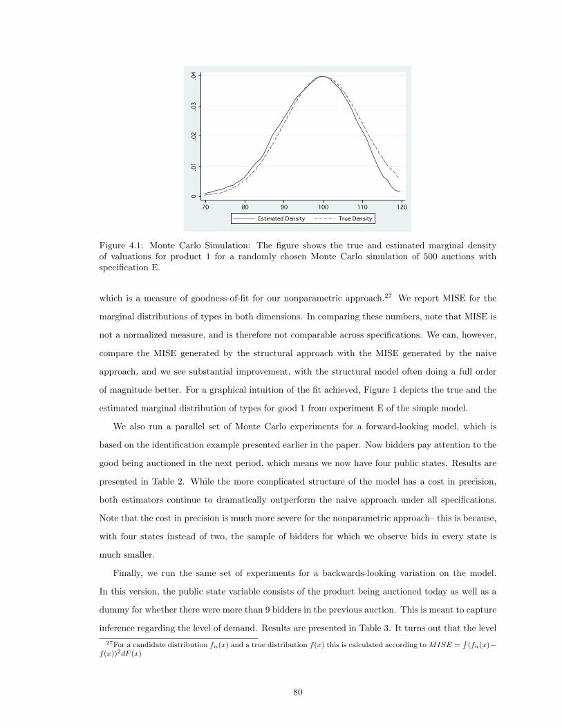
0.0
1.0
2.0
3.0
4
70 80 90 100 110 120
Estimated Density True Density
Figure 4.1: Monte Carlo Simulation: The figure shows the true and estimated marginal densityof valuations for product 1 for a randomly chosen Monte Carlo simulation of 500 auctions withspecification E.
which is a measure of goodness-of-fit for our nonparametric approach.27 We report MISE for the
marginal distributions of types in both dimensions. In comparing these numbers, note that MISE is
not a normalized measure, and is therefore not comparable across specifications. We can, however,
compare the MISE generated by the structural approach with the MISE generated by the naive
approach, and we see substantial improvement, with the structural model often doing a full order
of magnitude better. For a graphical intuition of the fit achieved, Figure 1 depicts the true and the
estimated marginal distribution of types for good 1 from experiment E of the simple model.
We also run a parallel set of Monte Carlo experiments for a forward-looking model, which is
based on the identification example presented earlier in the paper. Now bidders pay attention to the
good being auctioned in the next period, which means we now have four public states. Results are
presented in Table 2. While the more complicated structure of the model has a cost in precision,
both estimators continue to dramatically outperform the naive approach under all specifications.
Note that the cost in precision is much more severe for the nonparametric approach– this is because,
with four states instead of two, the sample of bidders for which we observe bids in every state is
much smaller.
Finally, we run the same set of experiments for a backwards-looking variation on the model.
In this version, the public state variable consists of the product being auctioned today as well as a
dummy for whether there were more than 9 bidders in the previous auction. This is meant to capture
inference regarding the level of demand. Results are presented in Table 3. It turns out that the level
27For a candidate distribution fn(x) and a true distribution f(x) this is calculated according to MISE =∫
(fn(x)−f(x))2dF (x)
80
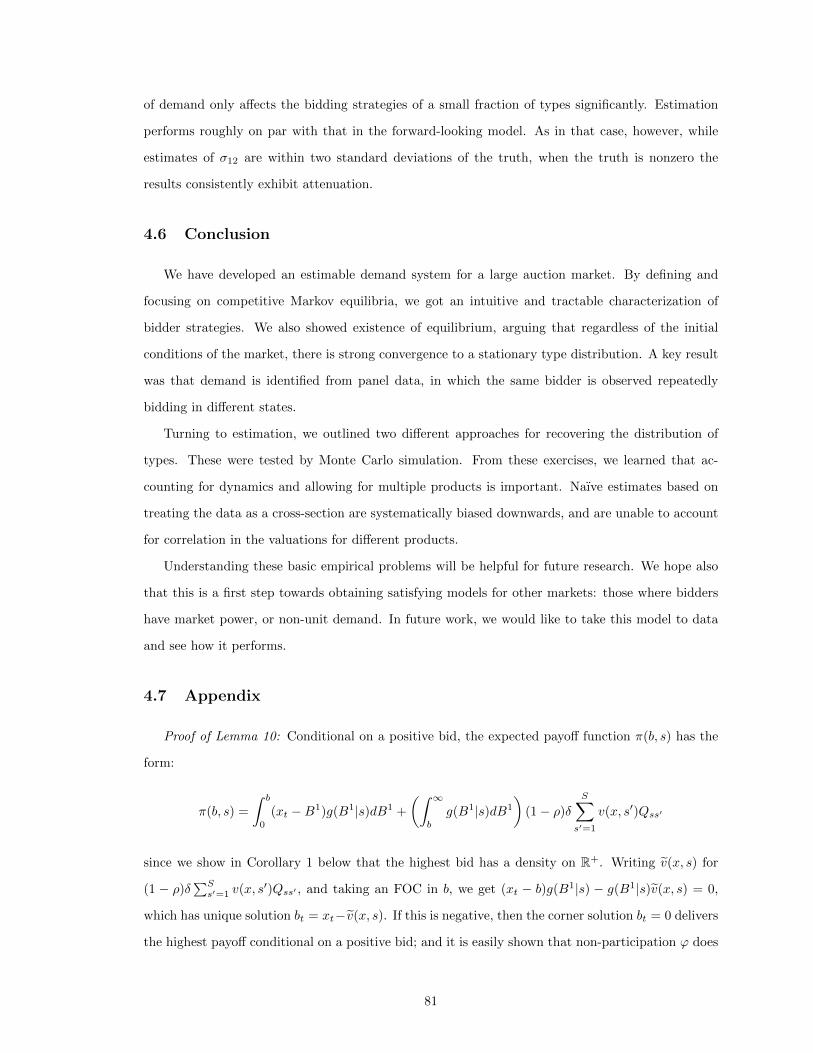
of demand only affects the bidding strategies of a small fraction of types significantly. Estimation
performs roughly on par with that in the forward-looking model. As in that case, however, while
estimates of σ12 are within two standard deviations of the truth, when the truth is nonzero the
results consistently exhibit attenuation.
4.6 Conclusion
We have developed an estimable demand system for a large auction market. By defining and
focusing on competitive Markov equilibria, we got an intuitive and tractable characterization of
bidder strategies. We also showed existence of equilibrium, arguing that regardless of the initial
conditions of the market, there is strong convergence to a stationary type distribution. A key result
was that demand is identified from panel data, in which the same bidder is observed repeatedly
bidding in different states.
Turning to estimation, we outlined two different approaches for recovering the distribution of
types. These were tested by Monte Carlo simulation. From these exercises, we learned that ac-
counting for dynamics and allowing for multiple products is important. Naıve estimates based on
treating the data as a cross-section are systematically biased downwards, and are unable to account
for correlation in the valuations for different products.
Understanding these basic empirical problems will be helpful for future research. We hope also
that this is a first step towards obtaining satisfying models for other markets: those where bidders
have market power, or non-unit demand. In future work, we would like to take this model to data
and see how it performs.
4.7 Appendix
Proof of Lemma 10: Conditional on a positive bid, the expected payoff function π(b, s) has the
form:
π(b, s) =
∫ b
0
(xt −B1)g(B1|s)dB1 +
(∫ ∞b
g(B1|s)dB1
)(1− ρ)δ
S∑s′=1
v(x, s′)Qss′
since we show in Corollary 1 below that the highest bid has a density on R+. Writing v(x, s) for
(1 − ρ)δ∑Ss′=1 v(x, s′)Qss′ , and taking an FOC in b, we get (xt − b)g(B1|s) − g(B1|s)v(x, s) = 0,
which has unique solution bt = xt−v(x, s). If this is negative, then the corner solution bt = 0 delivers
the highest payoff conditional on a positive bid; and it is easily shown that non-participation ϕ does
81

better still because the probability of winning with a bid of zero is positive (e.g. there may be no
other bidders in the market).
Proof of Lemma 11: By Theorem 11.12 in Stokey, Lucas, and Prescott (1989), uniform geometric
convergence in total variation norm will be achieved if their “condition M” holds: there exists ε > 0
and N ≥ 1 such that for all A ∈ F , either PN (ω,A) ≥ ε ω ∈ Ω or PN (ω,Ac) ≥ ε ∀ω ∈ Ω, for
PN the N -step transition probability. Let s0 = T (0,1) and ω0 = (0, s0) (i.e. ω0 is a superset of
the true state where there are no current participants, nor have been for the observable history;
and upcoming supply is entirely of object 1). Let p0 = P(Et = 0|Nt−1 = 0) > 0, by assumption;
let q0 = P(jt = 1); and let N0 = maxkf , kh + 1. Then PN0(ω, ω0) ≥ ρN (p0q0)N0 > 0 ∀ω ∈ Ω.
Choosing N = N0 and ε = ρN (p0q0)N0−1, condition M holds since either ω0 ∈ A or ω0 ∈ Ac.
Next, consider the marginal ergodic distribution on X N−1×S produced by integrating out the first
non-zero element of the type vector. Since S is finite, there is a well-defined conditional distribution
of x−i given s.
Proof of Theorem 1: Let the action space Ak be a finite grid ϕ, 0, xk ,2xk · · · x
S , with each
dimension totally ordered as written. Endow Ak with the Euclidean metric denoted d, where ϕ is
treated as having value −xk . Here, we define strategies as mappings from type to actions, β : X → Ak,
and write β(x) = (β1(x), β2(x) · · ·βS(x)). For each s, let λ(s) ∈ J be the object under auction in
state s; the mapping is well defined because of restriction (i) on the coarsening T. As in the text,
we call β monotone if βs(x) is increasing in xj if j = λ(s) and decreasing otherwise. Following Reny
(2008), let M denote the space of monotone functions from X to Ak, and define a metric δ on M
by:
δ(β, β′) =
∫Xd(β(x), β′(x))dµ(x)
As shown there, (M, δ) is a compact absolute retract. Define the payoff function u(a, t, β−i), equal
to the value of the game for type t when playing action vector a, everyone else follows strategy β−i,
and the invariant measure over true states is determined as though everyone plays β−i. As Reny
(2008) shows, the interim payoff function U(β, β−i) =∫X u(β(t), t, β−i)dµ(x) is continuous in both
arguments since the type distribution is atomless.
Let Γ(β−i) be the best response correspondence; by the theorem of the maximum it is non-empty
valued and upper-hemicontinuous. A fixed point of the correspondence, β∗, will be a CME, since
then strategies will be optimal given that the invariant measure over types is generated by play of
β∗. The existence of such a fixed point is guaranteed by the fixed point theorem due to Eilenberg
and Montgomery (1946) if we can show that Γ is contractible-valued and Γ(β−i) ∈ M whenever
82

β−i ∈M .
Fix β−i ∈ M and x ∈ X , and let v(x, s) still denote the ex-ante continuation value given
optimal actions. Then we can look at the optimal action state by state, and we have b∗s =
arg maxb∈Ak G1(b|s)(xλ(s) − E[B1|B1 ≤ b, s]) + (1 − G1(b|s))v(x, s). Define bls = maxbb : xλ(s) −
E[B1|B1 ≤ b, s] − v(x, s) > 0 and bus = minbb : xt − E[B1|B1 ≤ b, s] − v(x, s) < 0. Comparing
their payoffs directly, we see that bls yields higher payoff than bus ; this proves that these two bids
could not both be best responses. Next, at least one of these must be a best response — suppose
b < bls is optimal, then xt−E[B1|B1 ≤ b, s]− v(x, s) > 0; but since the payoff function is a weighted
sum of xt−E[B1|B1 ≤ b, s] and v(x, s), and G1(b|s) is (weakly) increasing in b for β−i ∈M , bls must
be weakly better still, and also a best response. The same argument holds on the other side. In
sum, either bls or bus (but not both) is part of the optimal strategy, and the best response is unique
unless G1(b|s) is constant over actions in some state (i.e. β−i assigns no mass to these actions).
Two results follow. First, since bls and bus are increasing in xλ(s) and decreasing in x−λ(s) —
since v increases in x−λ(s) — the best response to any β−i ∈ M is also in M . Second, given best
responses b and b′, the join b ∨ b′ is also a best response, since the probability of winning must be
constant over those actions, and so taking the coordinate-wise max doesn’t change payoffs at all. Γ
is thus join-closed and non-empty for β−i ∈M .
Finally, then, we need to construct a contraction on the best reply correspondence. We slightly
adapt Reny (2008) because actions are not increasing in type in all states. Fix β−i and (β, β0) ∈
Γ(β−i). Let Fi(x) be the marginal distribution of valuations for product i, and define functions
Φs(x) =Fλ(s)(x)−F−λ(s)(x)+1
2 , where F−λ(s)(x) is the average valuation quantile of objects not auc-
tioned at s. Then define
hs(τ, β)(x) =
βs(x), if Φs(x) ≤ |1− 2τ | and τ < 0.5
βs0(x), if Φs(x) ≤ |1− 2τ | and τ ≥ 0.5
βs0(x) ∨ βs(x), if Φs(x) > |1− 2τ |
Define h(τ, β)(x) = (h1(τ, β)(x), h2(τ, β)(x) · · ·hS(τ, β)(x)). It can be verified that h(τ, β) is mono-
tone, continuous and a best reply almost everywhere. This proves Γ contractible valued, and hence
it has a fixed point on M , showing existence for the finite action game.
To complete the proof, it suffices to show that there is a limiting set of strategies in which no
positive measure of types makes a bid b ∈ R+ in any state s (a positive measure of types bidding ϕ
presents no problems). But we showed earlier that for any grid fineness k, either bls or bus is played
83
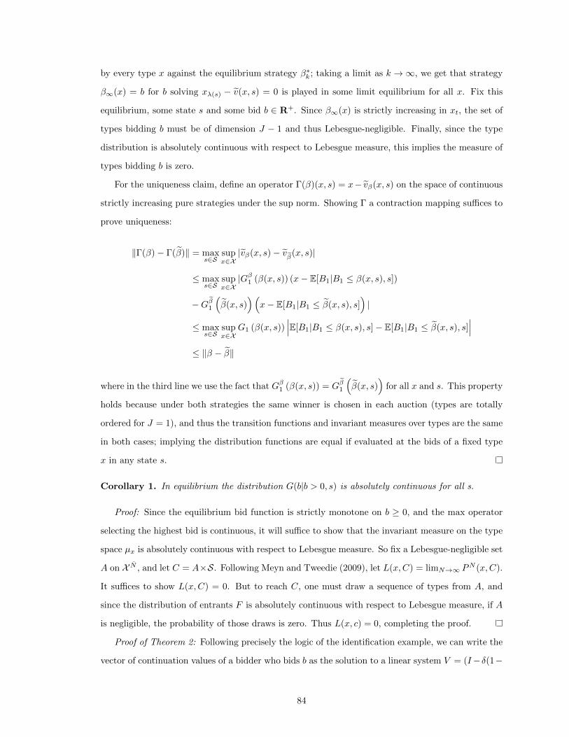
by every type x against the equilibrium strategy β∗k ; taking a limit as k →∞, we get that strategy
β∞(x) = b for b solving xλ(s) − v(x, s) = 0 is played in some limit equilibrium for all x. Fix this
equilibrium, some state s and some bid b ∈ R+. Since β∞(x) is strictly increasing in xt, the set of
types bidding b must be of dimension J − 1 and thus Lebesgue-negligible. Finally, since the type
distribution is absolutely continuous with respect to Lebesgue measure, this implies the measure of
types bidding b is zero.
For the uniqueness claim, define an operator Γ(β)(x, s) = x− vβ(x, s) on the space of continuous
strictly increasing pure strategies under the sup norm. Showing Γ a contraction mapping suffices to
prove uniqueness:
‖Γ(β)− Γ(β)‖ = maxs∈S
supx∈X|vβ(x, s)− vβ(x, s)|
≤ maxs∈S
supx∈X|Gβ1 (β(x, s)) (x− E[B1|B1 ≤ β(x, s), s])
−Gβ1(β(x, s)
)(x− E[B1|B1 ≤ β(x, s), s]
)|
≤ maxs∈S
supx∈X
G1 (β(x, s))∣∣∣E[B1|B1 ≤ β(x, s), s]− E[B1|B1 ≤ β(x, s), s]
∣∣∣≤ ‖β − β‖
where in the third line we use the fact that Gβ1 (β(x, s)) = Gβ1
(β(x, s)
)for all x and s. This property
holds because under both strategies the same winner is chosen in each auction (types are totally
ordered for J = 1), and thus the transition functions and invariant measures over types are the same
in both cases; implying the distribution functions are equal if evaluated at the bids of a fixed type
x in any state s.
Corollary 1. In equilibrium the distribution G(b|b > 0, s) is absolutely continuous for all s.
Proof: Since the equilibrium bid function is strictly monotone on b ≥ 0, and the max operator
selecting the highest bid is continuous, it will suffice to show that the invariant measure on the type
space µx is absolutely continuous with respect to Lebesgue measure. So fix a Lebesgue-negligible set
A on X N , and let C = A×S. Following Meyn and Tweedie (2009), let L(x,C) = limN→∞ PN (x,C).
It suffices to show L(x,C) = 0. But to reach C, one must draw a sequence of types from A, and
since the distribution of entrants F is absolutely continuous with respect to Lebesgue measure, if A
is negligible, the probability of those draws is zero. Thus L(x, c) = 0, completing the proof.
Proof of Theorem 2: Following precisely the logic of the identification example, we can write the
vector of continuation values of a bidder who bids b as the solution to a linear system V = (I−δ(1−
84
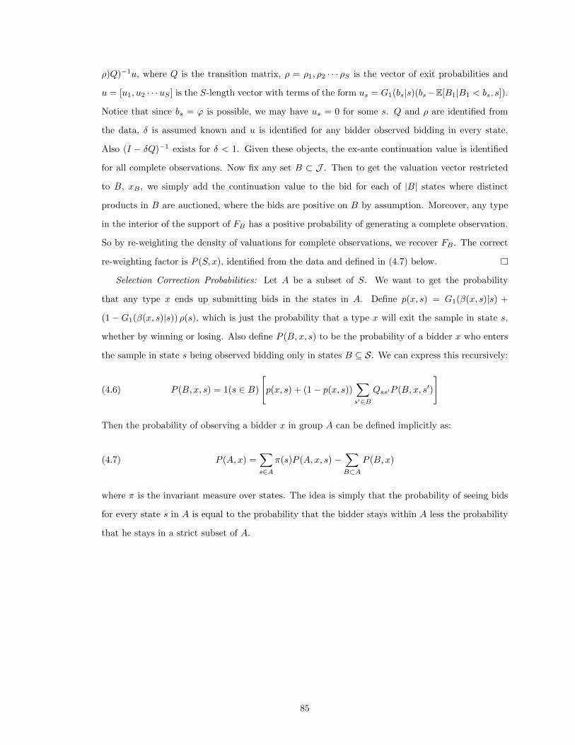
ρ)Q)−1u, where Q is the transition matrix, ρ = ρ1, ρ2 · · · ρS is the vector of exit probabilities and
u = [u1, u2 · · ·uS ] is the S-length vector with terms of the form us = G1(bs|s)(bs−E[B1|B1 < bs, s]).
Notice that since bs = ϕ is possible, we may have us = 0 for some s. Q and ρ are identified from
the data, δ is assumed known and u is identified for any bidder observed bidding in every state.
Also (I − δQ)−1 exists for δ < 1. Given these objects, the ex-ante continuation value is identified
for all complete observations. Now fix any set B ⊂ J . Then to get the valuation vector restricted
to B, xB , we simply add the continuation value to the bid for each of |B| states where distinct
products in B are auctioned, where the bids are positive on B by assumption. Moreover, any type
in the interior of the support of FB has a positive probability of generating a complete observation.
So by re-weighting the density of valuations for complete observations, we recover FB . The correct
re-weighting factor is P (S, x), identified from the data and defined in (4.7) below.
Selection Correction Probabilities: Let A be a subset of S. We want to get the probability
that any type x ends up submitting bids in the states in A. Define p(x, s) = G1(β(x, s)|s) +
(1−G1(β(x, s)|s)) ρ(s), which is just the probability that a type x will exit the sample in state s,
whether by winning or losing. Also define P (B, x, s) to be the probability of a bidder x who enters
the sample in state s being observed bidding only in states B ⊆ S. We can express this recursively:
(4.6) P (B, x, s) = 1(s ∈ B)
[p(x, s) + (1− p(x, s))
∑s′∈B
Qss′P (B, x, s′)
]
Then the probability of observing a bidder x in group A can be defined implicitly as:
(4.7) P (A, x) =∑s∈A
π(s)P (A, x, s)−∑B⊂A
P (B, x)
where π is the invariant measure over states. The idea is simply that the probability of seeing bids
for every state s in A is equal to the probability that the bidder stays within A less the probability
that he stays in a strict subset of A.
85
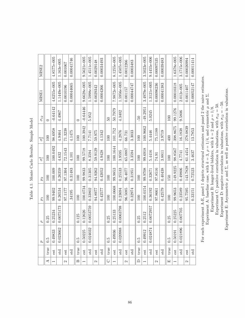
Tab
le4.1
:M
onte
Carl
oR
esu
lts:
Sim
ple
Mod
el
pρ
µ1
µ2
σ2 1
σ2 2
σ12
MIS
E1
MIS
E2
Atr
ue
0.5
0.25
100
100
100
100
0
1es
t0.
4983
30.
2523
499.9
402
100.0
09
100.0
492
98.6
958
-0.6
414
24.6
255e-
005
4.8
577e-
005
std
0.02
3662
0.00
7517
30.2
6534
0.2
6359
4.6
32
4.9
464
4.4
967
1.1
449e-
005
1.1
63e-
005
2es
t97.1
177
97.1
304
72.1
543
71.3
238
0.0
010196
0.0
01067
std
.34195
0.3
1483
4.1
01
4.1
475
0.0
0044665
0.0
0041746
Btr
ue
0.5
0.12
5100
100
100
100
0
1es
t0.
5022
50.
1262
6100.0
734
99.9
833
99.5
718
100.3
942
-0.6
444
69.6
628e-
005
9.5
621e-
005
std
0.02
4032
0.00
5375
90.3
3802
0.3
1305
8.3
594
7.7
141
5.9
52
1.5
998e-
005
1.4
511e-
005
2es
t94.8
977
94.9
262
59.9
129
59.9
75
0.0
029342
0.0
029148
std
0.4
2577
0.4
2052
4.9
428
4.1
342
0.0
004266
0.0
0034493
Ctr
ue
0.5
0.25
100
100
100
100
50
1es
t0.
4993
60.
2513
3100.0
668
99.9
853
100.1
644
101.7
52
50.7
979
7.9
872e-
005
8.1
255e-
005
std
0.02
0988
0.00
6379
80.2
3694
0.2
5533
3.9
595
4.2
876
4.3
402
1.5
956e-
005
1.4
507e-
005
2es
t96.5
085
96.4
077
65.0
887
66.7
31
0.0
01157
0.0
012266
std
0.3
2974
0.3
1951
3.3
594
3.3
033
0.0
0044747
0.0
003483
Dtr
ue
0.5
0.25
100
100
100
100
-50
1es
t0.
4991
20.
2512
100.0
154
99.9
708
99.6
918
100.9
662
-49.2
951
3.4
979e-
005
3.5
023e-
005
std
0.02
4874
0.00
7295
70.3
6192
0.3
2671
5.4
416
5.4
446
5.0
245
1.3
121e-
005
9.4
455e-
006
2es
t97.8
661
97.8
516
74.9
175.1
188
0.0
0096236
0.0
0097535
std
0.4
2579
0.4
0438
3.8
811
3.9
719
0.0
0041383
0.0
0039483
Etr
ue
0.5
0.25
100
150
100
400
100
1es
t0.
5019
10.
2522
599.9
653
149.9
225
98.8
567
398.8
675
99.1
276
0.0
0010318
1.6
378e-
005
std
0.02
1896
0.00
7705
0.2
3589
0.4
9806
4.7
741
16.1
838
9.5
806
2.0
12e-
005
3.1
715e-
006
2es
t95.7
595
143.7
828
61.4
454
278.0
839
0.0
011407
0.0
0026994
std
0.3
3151
0.7
2523
3.4
637
13.7
853
0.0
0052147
0.0
0011414
For
each
exp
erim
ent
A-E
,p
an
el1
dep
icts
stru
ctu
ral
esti
mate
san
dp
an
el2
the
naiv
ees
tim
ate
s.E
xp
erim
ent
A:
base
lin
eca
se,
wit
hk
=3,ρ
=1/
4,
an
dsy
mm
etri
cµ
an
dΣ
.E
xp
erim
ent
B:
lon
ger
-liv
edb
idd
ers,
wit
hk
=2
an
dρ
=1/
8.
Exp
erim
ent
C:
posi
tive
corr
elati
on
inva
luati
on
s,w
ithσ
12
=50.
Exp
erim
ent
D:
neg
ati
veco
rrel
ati
on
inva
luati
on
s,w
ithσ
12
=−
50.
Exp
erim
ent
E:
Asy
mm
etri
cµ
an
dΣ
,as
wel
las
posi
tive
corr
elati
on
inva
luati
on
s.
86

Tab
le4.2
:M
onte
Carl
oR
esu
lts:
Forw
ard
-Lookin
gM
od
el
pρ
µ1
µ2
σ2 1
σ2 2
σ12
MIS
E1
MIS
E2
Atr
ue
0.5
0.25
100
100
100
100
0
1es
t0.
4998
70.
2490
199.9
341
99.8
08
94.8
547
94.8
593
-1.4
892
0.0
0022831
0.0
0022285
std
0.02
1162
0.00
6513
10.2
871
0.2
9919
6.4
142
6.3
335
4.9
616
5.5
919e-
005
4.6
794e-
005
2es
t97.1
755
97.0
25
71.8
718
72.8
582
0.0
0068577
0.0
0063888
std
0.3
3698
0.3
3314
3.4
844
3.7
971
0.0
0034674
0.0
0033673
Btr
ue
0.5
0.12
5100
100
100
100
0
1es
t0.
4976
80.
1248
799.9
521
100.0
425
97.5
813
97.3
092
-2.9
59
0.0
0042409
0.0
0041063
std
0.02
3491
0.00
5788
50.3
9795
0.4
0503
7.9
82
9.1
703
6.1
737
8.0
64e-
005
7.7
461e-
005
2es
t94.9
433
95.0
142
59.7
917
59.2
406
0.0
019602
0.0
019706
std
0.4
0746
0.4
0215
4.5
596
4.3
055
0.0
0032758
0.0
0026379
Ctr
ue
0.5
0.25
100
100
100
100
50
1es
t0.
4941
0.25
058
99.8
19
99.8
049
91.8
484
92.6
894
42.9
742
0.0
003049
0.0
003044
std
0.02
6691
0.00
6902
40.3
072
0.2
8907
5.9
086
5.3
654
5.2
429
7.1
99e-
005
5.8
35e-
005
2es
t96.4
719
96.4
774
65.7
957
65.7
867
0.0
0083543
0.0
0081302
std
0.3
0472
0.3
4834
3.3
865
3.3
406
0.0
0034527
0.0
0035448
Dtr
ue
0.5
0.25
100
100
100
100
-50
1es
t0.
5036
90.
2507
999.9
49
100.0
644
96.3
282
97.4
392
-44.4
073
0.0
0023373
0.0
0023328
std
0.02
3882
0.00
6943
40.3
2751
0.3
21
8.1
597
8.5
975
5.6
176
5.9
192e-
005
6.2
75e-
005
2es
t97.7
889
97.9
007
75.2
727
75.6
323
0.0
0057612
0.0
0052678
std
0.3
6284
0.3
7382
4.0
511
4.6
602
0.0
0029306
0.0
0032672
Etr
ue
0.5
0.25
100
150
100
400
100
1es
t0.
5050
30.
2505
299.7
609
149.6
732
92.5
428
369.8
52
87.3
218
0.0
0035134
6.9
119e-
005
std
0.02
2175
0.00
6473
50.3
2631
0.5
5967
6.1
947
25.9
437
11.3
395
5.9
314e-
005
1.4
589e-
005
2es
t95.7
264
143.7
643
62.4
126
277.3
82
0.0
0082781
0.0
0019845
std
0.3
5323
0.6
1251
3.5
549
14.2
732
0.0
0041283
8.2
194e-
005
For
each
exp
erim
ent
A-E
,p
an
el1
dep
icts
stru
ctu
ral
esti
mate
san
dp
an
el2
the
naiv
ees
tim
ate
s.E
xp
erim
ent
A:
base
lin
eca
se,
wit
hk
=3,ρ
=1/
4,
an
dsy
mm
etri
cµ
an
dΣ
.E
xp
erim
ent
B:
lon
ger
-liv
edb
idd
ers,
wit
hk
=2
an
dρ
=1/
8.
Exp
erim
ent
C:
posi
tive
corr
elati
on
inva
luati
on
s,w
ithσ
12
=50.
Exp
erim
ent
D:
neg
ati
veco
rrel
ati
on
inva
luati
on
s,w
ithσ
12
=−
50.
Exp
erim
ent
E:
Asy
mm
etri
cµ
an
dΣ
,as
wel
las
posi
tive
corr
elati
on
inva
luati
on
s.
87

Tab
le4.3
:M
onte
Carl
oR
esu
lts:
Back
ward
-Lookin
gM
od
el
pρ
µ1
µ2
σ2 1
σ2 2
σ12
MIS
E1
MIS
E2
Atr
ue
0.5
0.25
100
100
100
100
0
1es
t0.
5022
50.
2490
399.5
455
99.4
76
90.5
713
90.0
723
0.8
1214
0.0
0030105
0.0
0032009
std
0.02
2929
0.00
6675
70.2
83
0.2
9668
7.5
447
7.9
162
4.8
788
9.6
654e-
005
0.0
0010594
2es
t97.0
564
97.0
128
66.3
069
66.7
998
0.0
011306
0.0
01079
std
0.3
4049
0.3
4873
3.3
928
3.9
655
0.0
0039424
0.0
0047592
Btr
ue
0.5
0.12
5100
100
100
100
0
1es
t0.
5054
30.
126
99.4
281
99.2
61
94.1
747
93.1
985
-0.9
9954
0.0
0057706
0.0
0060249
std
0.01
8153
0.00
5335
10.3
7785
0.3
5817
9.5
136
10.7
578
6.7
87
0.0
0015555
0.0
0015446
2es
t94.8
876
94.8
948
56.1
622
55.3
11
0.0
030883
0.0
031265
std
0.3
7063
0.3
8293
4.6
828
4.2
582
0.0
0045435
0.0
0048513
Ctr
ue
0.5
0.25
100
100
100
100
50
1es
t0.
5014
0.24
894
99.4
041
99.3
418
89.3
272
89.2
724
41.2
166
0.0
0035513
0.0
0037807
std
0.02
1388
0.00
6063
80.2
7722
0.2
6244
7.4
923
7.6
598
5.9
907
9.6
62e-
005
9.3
648e-
005
2es
t96.3
922
96.3
618
61.9
956
61.7
951
0.0
013294
0.0
013081
std
0.3
4935
0.2
6843
3.4
279
3.4
378
0.0
0033777
0.0
0045434
Dtr
ue
0.5
0.25
100
100
100
100
-50
1es
t0.
5013
10.
2489
899.7
147
99.5
963
92.1
85
90.9
354
-40.2
983
0.0
0031033
0.0
0033724
std
0.02
4505
0.00
6184
30.3
2289
0.3
0584
8.3
661
7.6
269
5.7
865
0.0
0010573
9.9
659e-
005
2es
t97.8
232
97.7
51
68.4
931
68.5
974
0.0
011092
0.0
0095543
std
0.3
5707
0.3
6555
3.4
815
4.2
274
0.0
0030701
0.0
0044662
Etr
ue
0.5
0.25
100
150
100
400
100
1es
t0.
5011
50.
2501
499.2
897
148.9
155
88.1
829
363.6
608
83.7
978
0.0
0040269
8.7
667e-
005
std
0.02
2705
0.00
6559
70.2
8836
0.5
3591
8.3
556
27.3
134
11.0
149
9.2
293e-
005
2.3
743e-
005
2es
t95.9
237
143.5
118
59.2
387
258.8
469
0.0
012831
0.0
0028309
std
0.3
2372
0.6
5581
3.7
201
13.1
16
0.0
0040399
0.0
001278
For
each
exp
erim
ent
A-E
,p
an
el1
dep
icts
stru
ctu
ral
esti
mate
san
dp
an
el2
the
naiv
ees
tim
ate
s.E
xp
erim
ent
A:
base
lin
eca
se,
wit
hk
=3,ρ
=1/
4,
an
dsy
mm
etri
cµ
an
dΣ
.E
xp
erim
ent
B:
lon
ger
-liv
edb
idd
ers,
wit
hk
=2
an
dρ
=1/
8.
Exp
erim
ent
C:
posi
tive
corr
elati
on
inva
luati
on
s,w
ithσ
12
=50.
Exp
erim
ent
D:
neg
ati
veco
rrel
ati
on
inva
luati
on
s,w
ithσ
12
=−
50.
Exp
erim
ent
E:
Asy
mm
etri
cµ
an
dΣ
,as
wel
las
posi
tive
corr
elati
on
inva
luati
on
s.
88

CHAPTER V
Conclusion
The three chapters of this dissertation have endeavored to show the importance and the flexibility
of dynamic modeling of economic behavior, both for empirical and analytic work.
Chapter 1 demonstrated that a dynamic model of firm selection is empirically separable from the
familiar notion of X-inefficiency, and developed methods with an application to Ready-Mix Concrete
data from the US Census of Manufactures. X-inefficiency was vindicated as the primary explanation
for the stylized fact that productivity and competition are correlated.
Chapter 2 demonstrated that comparative statics can be derived from general industry dynamics
models without the imposition of parametric form. Results were obtained for firm turnover rates
and average type with respect to changes in fixed costs of entry and market size.
Finally, Chapter 3 posited a dynamic model of an auction marketplace, meant to represent the
eBay platform, and demonstrated both the viability and, in monte carlo simulations, the importance
of incorporating dynamic considerations in demand estimation for this environment.
It is the hope of the author that these contributions will spur future innovation in general,
dynamic analysis.
89

BIBLIOGRAPHY
90

BIBLIOGRAPHY
Ackerberg, D. (2003): “Advertising, Learning, and Consumer Choice in Experience Good Markets: AnEmpirical Examination,” International Economic Review, 44(3), 1007–1040.
(2009): “Quantitative Marketing and Economics,” A New Use of Importance Sampling to ReduceComputational Burden in Simulation Estimation, 7(4), 343–376.
Ackerberg, D., K. Caves, and G. Frazer (2006): “Structural Identification of Production Functions,”Working Paper.
Ackerberg, D., K. Hirano, and Q. Shahriar (2011): “Identification of Time and Risk Preferencesin Buy Price Auctions,” Working Paper.
Adams, C. (2012): “Identifying Demand from Online Auction Data,” Working Paper.
Ai, C., and X. Chen (2003): “Efficient Estimation of Models with Conditional Moment RestrictionsContaining Unknown Functions,” Econometrica, 71(6), 1795–1843.
Alchian, A. A. (1950): “Uncertainty, Evolution, and Economic Theory,” Journal of Political Economy,58(3), 211–221.
Andrews, D. (1994): “Asymptotics for Semiparametric Econometric Models Via Stochastic Equiconti-nuity,” Econometrica, 62(1), 43–72.
Asplund, M., and V. Nocke (2006): “Firm Turnover in Imperfectly Competitive Markets,” Review ofEconomic Studies, 73(2), 295–327.
Athey, S. (2000): “Characterizing Properties of Schochastic Objective Functions,” Working Paper.
(2001): “Single Crossing Properties and the Existence of Pure Strategy Equilibria in Games ofIncomplete Information,” Econometrica, 69(4), 861–889.
Athey, S., and P. Haile (2002): “Identification of Standard Auction Models,” Econometrica, 70(6),2107–2140.
Backus, M. R. (2011): “Why is Productivity Correlated with Competition?,” Working Paper.
Bajari, P., L. Benkard, and J. Levin (2007): “Estimating Dynamic Models of Imperfect Competi-tion,” Econometrica, 75(5), 1331–1370.
Bajari, P., and A. Hortacsu (2004): “Economic Insights from Internet Auctions,” Econometrica,42(2), 457–486.
Berger, A. N., and T. H. Hannan (1998): “The Efficiency Cost of Market Power in the BankingIndustry: A Test of the ”Quiet Life” and Related Hypotheses,” The Review of Economics andStatistics, 80(3), 454–465.
Berry, S. (1994): “Estimating Discrete Choice Models of Product Differentiation,” RAND Journal ofEconomics, 25, 242–262.
91
Berry, S., J. Levinsohn, and A. Pakes (1995): “Automobile Prices in Market Equilibrium,” Econo-metrica, 63(4), 841–890.
(2004): “Differentiated Products Demand Systems from a Combination of Micro and MacroData: The New Car Market,” The Journal of Political Economy, pp. 68–105.
Bond, S., and M. Sderbom (2005): “Adjustment Costs and the Identification of Cobb Douglas Pro-duction Functions,” Working Paper.
Boone, J. (2008): “Competition: Theoretical Parameterization and Empirical Measures,” Journal ofInstitutional and Theoretical Economics, 164, 587–611.
Budish, E. (2012): “Sequencing and Information Revelation in Auctions for Imperfect Substitutes: Un-derstanding eBay’s Market Design,” Working Paper.
Caves, R., and D. Barton (1990): Efficiency in US Manufacturing Industries. MIT Press.
Chen, X. (2007): Handbook of Econometricsvol. 6, chap. Large Sample Sieve Estimation of Semi-Nonparametric Models. Elsevier, 1 edn.
Collard-Wexler, A. (2011): “Productivity Dispersion and Plant Selection in the Ready-Mix ConcreteIndustry,” CES Working Paper 11-25.
Combes, P., G. Duranton, L. Gobillon, D. Puga, and S. Roux (2010): “The Productivity Ad-vantages of Large Cities: Distinguishing Agglomeration from Firm Selection,” Working Paper.
Doraszelski, U., and M. Satterthwaite (2010): “Computable Markov-Perfect Industry Dynamics,”RAND Journal of Economics, 41(2), 215–243.
Duffie, D., J. Geanakoplos, A. Mas-Colell, and A. McLennan (1994): “Stationary MarkovEquilibria,” Econometrica, 62(4), 745–781.
Dunne, T., S. Klimek, and J. Schmitz (2010): “Competition and Productivity: Evidence from thePost-WWII US Cement Industry,” CES Working Paper 10-23.
Eilenberg, S., and D. Montgomery (1946): “Fixed Point Theorems for Multi-Valued Transforma-tions,” American Journal of Mathematics, 68, 214–222.
Ericson, R., and A. Pakes (1995): “Markov-Perfect Industry Dynamics: A Framework for EmpiricalWork,” The Review of Economic Studies, 62(1), 53–82.
Fersthman, C., and A. Pakes (2009): “Finite State Dynamic Games with Asymmetric Information:A Framework for Applied Work,” Working Paper.
Foster, L., J. Haltiwanger, and C. Syverson (2008): “Reallocation, Firm Turnover, and Efficiency:Selection on Productivity or Profitability?,” American Economic Review, 98(1), 394–425.
Gowrisankaran, G., and M. Rysman (2009): “Dynamics of Consumer Demand for New DurableGoods,” Working Paper.
Green, A., and D. Mayes (1991): “Technical Inefficiency in Manufacturing Industries,” The EconomicJournal, 101(406), 523–538.
Guerre, E., I. Perrigne, and Q. Vuong (2000): “Optimal Nonparametric Estimation of First-PriceAuctions,” Econometrica, 68(3), 525–574.
Hansen, L. P. (1982): “Large Sample Properties of Generalized Method of Moments Estimators,” Econo-metrica, 50, 1029–1054.
Harberger, A. C. (1954): “Monopoly and Resource Allocation,” American Economic Review, 44(2),77–87.
92

Hay, D. A., and G. S. Liu (1997): “The Efficiency of Firms: What Difference Does Competition Make?,”The Economic Journal, 107(442), 597–617.
Heckman, J. J. (1979): “Sample Selection Bias as Specification Error,” Econometrica, 47(1), 153–161.
Hendricks, K., and R. Porter (2007): “A Survey of Empirical Work in Auctions,” in Handbook ofIndustrial Organization, ed. by M. Armstrong, and R. Porter, vol. III. North-Holland.
Hopenhayn, H. (1992a): “Entry, Exit, and Firm Dynamics in Long Run Equilibrium,” Econometrica,60(5), 1127–1150.
(1992b): “Exit, Selection, and the Value of Firms,” Journal of Economic Dynamics and Control,16, 621–653.
Ingster, A. (2009): “A Structural Study of a Dynamic Auction Market,” Working Paper.
Jofre-Benet, M., and M. Pesendorfer (2003): “Econometrica,” Estimation of a Dynamic AuctionGame, 71(1), 1443–1489.
Johnson, K., and J. Kort (2004): “2004 Redefinition of the BEA Economic Areas,” Survey of CurrentBusiness, 84(11).
Jovanovic, B., and R. Rosenthal (1988): “Anonymous Sequential Games,” Journal of MathematicalEconomics, 17(1), 77–87.
Krusell, P., and A. A. Smith (1998): “Income and Wealth Heterogeneity in the Macroeconomy,” TheJournal of Political Economy, 106(5), 867–896.
Leibenstein, H. (1966): “Allocative Efficiency vs. ”X-Efficiency”,” American Economic Review, 56(3),392–425.
(1978): “X-Inefficiency Xists: Reply to an Xorcist,” The American Economic Review, 68(1),203–211.
Li, T., and Q. Vuong (1998): “Nonparametric Estimation of the Measurement Error Model UsingMultiple Indicators,” Journal of Multivariate Analysis, 65, 135–165.
Lippman, S., and R. Rumelt (1982): “Uncertain Imitability: An Analysis of Interfirm Differences inEfficiency under Competition,” The Bell Journal of Economics, 13(2), 418–438.
McFadden, D. (1974): “Conditional Logit Analysis of Qualitative Choice Behavior,” in Frontiers inEconometrics, ed. by P. Zarembka, pp. 105–142. Academic Press.
Melitz, M. (2003): “The Impact of Trade on Intra-Industry Reallocations and Aggregate IndustryProductivity,” Econometrica, 71(6), 1695–1725.
Melitz, M., and G. Ottaviano (2008): “Market Size, Trade, and Productivity,” Review of EconomicStudies, 75, 295–316.
Meyn, S., and R. Tweedie (2009): Markov Chains and Stochastic Stability. Cambridge UniversityPress.
Milgrom, P., and R. Weber (2000): “A Theory of Auctions and Competitive Bidding II,” in TheEconomic Theory of Auctions, ed. by P. Klemperer. Edward Elgar Publishing Ltd.
Mookherjee, D. (1983): “Optimal Incentive Schemes with Many Agents,” The Review of EconomicStudies, 51(3), 433–446.
Nalebuff, B., and J. Stiglitz (1983): “Prizes and Incentives: Towards a General Theory of Compen-sation and Competition,” The Bell Journal of Economics, 14(1), 21–43.
93

Nickell, S. J. (1996): “Competition and Corporate Performance,” Journal of Political Economy, 104(4),724–746.
Olley, S., and A. Pakes (1996): “The Dynamics of Productivity in the Telcommunications EquipmentIndustry,” Econometrica, 64(6), 1263–1297.
Pakes, A., M. Ostrovsky, and S. Berry (2007): “RAND Journal of Economics,” Simple Estimatorsfor the Parameters of Discrete Dynamic Games, with Entry/Exit Examples, 38(2), 373–399.
Pakes, A., and D. Pollard (1989): “Simulation and the Asymptotics of Optimization Estimators,”Econometrica, 57(5), 1027–1057.
Pavcnik, N. (2002): “Trade Liberalization, Exit, and Productivity Improvements: Evidence from ChileanPlants,” Review of Economic Studies, 69(1), 245–276.
Pesendorfer, M., and P. Schmidt-Dengler (2003): “Identification and Estimation of DynamicGames,” Working Paper.
Raith, M. (2003): “Competition, Risk, and Managerial Incentives,” The American Economic Review,93(4), 1425–1436.
Reny, P. (2008): “On the Existence of Monotone Equilibria in Bayesian Games,” Working Paper.
Said, M. (2012): “Auctions with Dynamic Populations: Efficiency and Revenue Maximization,” WorkingPaper.
Sailer, K. (2012): “Searching the eBay Marketplace,” Working Paper.
Satterthwaite, M., and A. Shneyerov (2007): “Dynamic Matching, Two-Sided Incomplete Informa-tion and Participation Costs: Existence and Convergence to Perfect Competition,” Econometrica,75(1), 155–200.
Schmidt, K. M. (1997): “Managerial Incentives and Product Market Competition,” The Review ofEconomic Studies, 64(2), 191–213.
Schmitz, J. A. (2005): “What Determines Productivity? Lessons from the Dramatic Recovery of theUS and Canadian Iron Ore Industries Following Their Early 1980s Crisis,” Journal of PoliticalEconomy, 113(3), 582–625.
Stigler, G. (1976): “The Xistence of X-Efficiency,” The American Economic Review, 66(1), 213–216.
Stokey, N., R. Lucas, and E. Prescott (1989): Recursive Methods in Economic Dynamics. HarvardUniversity Press.
Sutton, J. (1991): Sunk Costs and Market Structure. MIT Press.
Syverson, C. (2004): “Market Structure and Productivity: A Concrete Example,” Journal of PoliticalEconomy, 112(6), 1181–1222.
(2008): “Markets: Ready-Mix Concrete,” Journal of Economic Perspectives, 22(1), 217–233.
Vives, X. (2009): “Strategic Complementarity in Multi-Stage Games,” Economic Theory, 40(1), 151–171.
Weintraub, G., L. Benkard, and B. Van Roy (2008): “Markov Perfect Industry Dynamics withMany Firms,” Econometrica, 76(6), 1375–1411.
Williamson, O. (1968): “Economics as an Antitrust Defense: The Welfare Tradeoffs,” American Eco-nomic Review, 58(1), 18–36.
Wolinsky, A. (1988): “Dynamic Markets with Competitive Bidding,” The Review of Economic Studies,55(1), 71–84.
94

Zeithammer, R. (2006): “Forward-Looking Bidding in Online Auctions,” Journal of Marketing Research,43(3), 462–476.
(2012): “Sequential Auctions with Information About Future Goods,” Working Paper.
95