essays in empirical industrial organization

Essays in Empirical IndustrialOrganization

c©Peng Xue

ORCID ID: 0000-0003-0789-3174

Not to be cited or quoted without the authors permission

Submitted in ful�llment of the requirements for the degree of

Doctor of Philosophy (Economics)

Department of Economics

University of Melbourne

17 March 2020

Dedication

I dedicate this thesis to my dear mother who has loved me unreservedly since the �rst day

of my life.

1

Acknowledgments

I am immensely grateful to my supervisors David Byrne and Joe Hirschberg for their in-

valuable guidance and unwavering support. I am also grateful to the department's PhD

Director Kalvinder Shields for her constant encouragement and advice. I also thank Kevin

Staub, May Li, Simon Loetscher, Steve Puller and participants at the 2018 Australian Con-

ference of Economists and 2018 Asia-Paci�c Industrial Organization Conference for their

many useful comments. This research is supported by an Australian Government Research

Training Program (RTP) Scholarship. All errors are of my own.

2

Declaration

All work contained in this thesis has not been previously submitted to meet requirements

for a degree at this or any other higher education institution. The thesis contains only my

original work except where due reference is made. Due acknowledgment has been made in

the thesis to all material used. The thesis is no more than 100,000 words in length, exclusive

of tables, appendices and bibliographies.

��

Peng Xue

3

Abstract

This dissertation studies pricing behavior in the retail gasoline market. The main research

questions are: How does tra�c congestion a�ect market power of gas stations? How does

tra�c congestion a�ect equilibrium price dispersion between gas stations? Is gasoline price

cycle consistent with Edgeworth Cycle in terms of how their shapes respond to aggregate

demand elasticity? These questions are explored in three separate chapters respectively

using unique datasets comprised of station-level gasoline price data and direction-speci�c

road-level tra�c data from metropolitan Sydney and the rest of New South Wales.

Evidence from chapter 2 suggests that tra�c congestion, through its impact on spatial

friction for consumers, dampens the intensity of price competition between gas stations. By

exploiting a panel of 61 gasoline stations on 13 roads in Metropolitan Sydney, it is found that

the margins of regular gasoline increased with travel delay in local tra�c. Speci�cally, retail

margins of regular gasoline increased by 0.32 cents per liter (4%) when travel delay in local

tra�c has increased unexpectedly by 1 minute per kilometer. Unique to this paper is the

high-frequency nature of its data which allows me to examine how fast gasoline companies

are responding to spatial frictions at the hourly resolution. Analysis based on a dynamic

model suggests that this response is �instantaneous� as margins rise as early as the same

hour when a shock in tra�c congestion is observed.

In chapter 3, tra�c congestion is found to have an impact on equilibrium price dispersion

between gas stations. Motivated by empirical evidence that the majority of consumers search

for cheaper fuel while they drive, I exploit variation in tra�c delay to identify the e�ect of

consumer search cost on price dispersion in the equilibrium retail gasoline market. I �nd

4

that the relationship between price dispersion of regular gasoline and search cost is indeed

non-monotonic (inverse U-shaped). This �nding is consistent with the consumer search

model by a consumer search model presented in the chapter which predicts no dispersion

at the extremes: market prices converge to marginal cost when search cost approaches zero

and to the monopoly price when search cost approaches the upper bound. I �nd that at

the sample average level of tra�c delay (0.387 Min/KM) in New South Wales, pricing for

regular gasoline is more consistent with competitive pricing, but becomes more monopolistic

once tra�c delay rises above 1.20 Min/KM.

Finally in chapter 4, I establish new empirical evidence which suggests that gasoline

price cycles are consistent with Edgeworth Cycles. Using daily station-level price data for

regular gasoline over 2 years, I �nd that a higher price than a reference-price at the start

of a gasoline price cycle has an positive e�ect on cycle length and a negative e�ect on

undercutting aggressiveness. Based on established empirical evidence that gasoline demand

is reference-dependent and the predicted pricing response to aggregate demand elasticity

under the Edgeworth Cycle equilibrium, I infer from these results that the shape of a

gasoline price cycle depends on aggregate demand elasticity the same way the shape of a

Edgeworth Cycle does.

Insights from this dissertation can inform public agencies who are concerned with ad-

dressing the issue of tra�c congestion and regulators who are concerned with competition

and pricing behavior in the retail gasoline industry.

5

Contents

1 Introduction 12

1.1 Motivation . . . . . . . . . . . . . . . . . . . . . . . . . . . . . . . . . . . . . 12

1.2 Research questions . . . . . . . . . . . . . . . . . . . . . . . . . . . . . . . . . 13

1.3 Findings and Policy Implications . . . . . . . . . . . . . . . . . . . . . . . . . 15

2 Tra�c Congestion and Market Competition:

Evidence from the Retail Gasoline Market 17

2.1 Introduction . . . . . . . . . . . . . . . . . . . . . . . . . . . . . . . . . . . . . 17

2.2 How does tra�c congestion a�ect competition? . . . . . . . . . . . . . . . . . 19

2.3 Industry and data . . . . . . . . . . . . . . . . . . . . . . . . . . . . . . . . . 21

2.3.1 The retail gasoline market in Sydney, Australia . . . . . . . . . . . . 21

2.3.2 Data sources and variable construction . . . . . . . . . . . . . . . . . . 22

2.3.2.1 Price data . . . . . . . . . . . . . . . . . . . . . . . . . . . . 22

2.3.2.2 Tra�c data . . . . . . . . . . . . . . . . . . . . . . . . . . . . 22

2.3.3 Overview of data . . . . . . . . . . . . . . . . . . . . . . . . . . . . . . 24

2.3.4 Descriptive evidence . . . . . . . . . . . . . . . . . . . . . . . . . . . . 25

2.4 Methodology . . . . . . . . . . . . . . . . . . . . . . . . . . . . . . . . . . . . 25

2.5 Results . . . . . . . . . . . . . . . . . . . . . . . . . . . . . . . . . . . . . . . . 27

2.5.1 Main results . . . . . . . . . . . . . . . . . . . . . . . . . . . . . . . . . 27

2.5.2 E�ect on other types of gasoline . . . . . . . . . . . . . . . . . . . . . 28

2.5.3 E�ect by station brand . . . . . . . . . . . . . . . . . . . . . . . . . . 29

6

2.5.4 Dynamic e�ects of tra�c congestion . . . . . . . . . . . . . . . . . . . 30

2.6 Alternative explanations for the e�ect tra�c congestion on gasoline margins 32

2.7 Chapter conclusion . . . . . . . . . . . . . . . . . . . . . . . . . . . . . . . . . 33

3 Is the E�ect of Consumer Search Cost on Price

Dispersion Non-monotonic? Evidence from

the Retail Gasoline Industry 46

3.1 Related literature . . . . . . . . . . . . . . . . . . . . . . . . . . . . . . . . . 49

3.2 Tra�c congestion and consumer search cost - a conceptual framework . . . . 50

3.2.1 The Model . . . . . . . . . . . . . . . . . . . . . . . . . . . . . . . . . 51

3.3 Data and Descriptive Evidence . . . . . . . . . . . . . . . . . . . . . . . . . . 53

3.3.1 Tra�c data . . . . . . . . . . . . . . . . . . . . . . . . . . . . . . . . . 53

3.3.2 Measuring tra�c congestion . . . . . . . . . . . . . . . . . . . . . . . . 53

3.3.3 Price data . . . . . . . . . . . . . . . . . . . . . . . . . . . . . . . . . . 54

3.3.4 Measuring price dispersion . . . . . . . . . . . . . . . . . . . . . . . . 54

3.4 Methodology and results . . . . . . . . . . . . . . . . . . . . . . . . . . . . . . 57

3.4.1 Estimation strategy . . . . . . . . . . . . . . . . . . . . . . . . . . . . 57

3.5 Estimation results . . . . . . . . . . . . . . . . . . . . . . . . . . . . . . . . . 59

3.5.1 Non-parametric evidence of the inverse-U relationship . . . . . . . . . 60

3.5.2 Mechanism - opportunity cost of time . . . . . . . . . . . . . . . . . . 61

3.6 Robustness tests . . . . . . . . . . . . . . . . . . . . . . . . . . . . . . . . . . 62

3.6.1 Alternative measures of price dispersion . . . . . . . . . . . . . . . . . 62

3.6.2 Raw prices . . . . . . . . . . . . . . . . . . . . . . . . . . . . . . . . . 63

3.6.3 Dropping extreme tra�c delay . . . . . . . . . . . . . . . . . . . . . . 63


4 Reference-Dependent Demand, Price Cycle and

Competition in Retail Gasoline Market 77

4.1 Introduction . . . . . . . . . . . . . . . . . . . . . . . . . . . . . . . . . . . . . 77

4.2 Literature and hypotheses . . . . . . . . . . . . . . . . . . . . . . . . . . . . 79

7

4.3 Data . . . . . . . . . . . . . . . . . . . . . . . . . . . . . . . . . . . . . . . . . 81

4.3.1 Data source . . . . . . . . . . . . . . . . . . . . . . . . . . . . . . . . 81

4.3.2 Identifying stations with price cycles . . . . . . . . . . . . . . . . . . . 81

4.3.3 Measuring price cycle length . . . . . . . . . . . . . . . . . . . . . . . 82

4.3.4 Inferring aggregate demand elasticity of gasoline . . . . . . . . . . . . 84

4.3.4.1 De�nition of local gasoline markets . . . . . . . . . . . . . . 85

4.3.4.2 De�nition of reference-price . . . . . . . . . . . . . . . . . . . 85

4.3.5 Variables for characterizing within-cycle price dynamics . . . . . . . . 87

4.3.6 Visualizing the hypotheses . . . . . . . . . . . . . . . . . . . . . . . . 88

4.3.7 Descriptive evidence . . . . . . . . . . . . . . . . . . . . . . . . . . . . 89

4.4 Panel Analysis . . . . . . . . . . . . . . . . . . . . . . . . . . . . . . . . . . . 89

4.4.1 Empirical model for estimating the impact on cycle length . . . . . . . 89

4.4.2 Estimated impact on cycle length . . . . . . . . . . . . . . . . . . . . . 91

4.4.3 Empirical model for estimating the impact on undercutting aggres-

siveness . . . . . . . . . . . . . . . . . . . . . . . . . . . . . . . . . . . 91

4.4.4 Heterogeneous responses by brand . . . . . . . . . . . . . . . . . . . . 93

4.4.5 Robustness to alternative de�nitions of reference-price . . . . . . . . . 94


5 Conclusion 107

8

List of Figures

2.1 GEOGRAPHIC LOCATIONS OF SAMPLED GAS STATIONS SHOWN

ON GOOGLE MAP . . . . . . . . . . . . . . . . . . . . . . . . . . . . . . . . 36

2.2 GASOLINE PRICE CYCLES IN THE DATA . . . . . . . . . . . . . . . . . . 37

2.3 TRAFFIC CONGESTION BY DIRECTION AND TIME OF DAY . . . . . 38

2.4 DESCRIPTIVE EVIDENCE - BINNED SCATTER PLOT OF GASOLINE

MARGIN ON TRAFFIC DELAY . . . . . . . . . . . . . . . . . . . . . . . . 39

2.5 THE EFFECT OF FUTURE, CURRENT AND PAST TRAFFIC DELAY

ON CURRENT GASOLINE MARGINS . . . . . . . . . . . . . . . . . . . . 40

3.1 SEARCH COST (s) AND GAINS FROM SEARCH . . . . . . . . . . . . . . 66

3.2 ROADS REPORT . . . . . . . . . . . . . . . . . . . . . . . . . . . . . . . . . 67

3.3 TWO EXAMPLES OF LOCAL MARKET . . . . . . . . . . . . . . . . . . . 68

3.4 NET RELATIONSHIP BETWEEN TRAFFIC DELAY AND GAINS FROM

SEARCH . . . . . . . . . . . . . . . . . . . . . . . . . . . . . . . . . . . . . . 69

3.5 BINNED SCATTERPLOT OF of GS ON Delay . . . . . . . . . . . . . . . 70

3.6 NET RELATIONSHIP BETWEEN TRAFFIC DELAY AND GAINS FROM

SEARCH BY GASOLINE TYPE . . . . . . . . . . . . . . . . . . . . . . . . 71

3.7 ROBUSTNESS TEST - ALTERNATIVE MEASURES OF PRICE DISPER-

SION . . . . . . . . . . . . . . . . . . . . . . . . . . . . . . . . . . . . . . . . 72

3.8 ROBUSTNESS TEST - RAW PRICES . . . . . . . . . . . . . . . . . . . . . 73

3.9 ROBUSTNESS TEST - DROPPING EXTREME TRAFFIC DELAY . . . . 74

9

4.1 DYNAMIC PRICE PATH OF CYCLING STATIONS . . . . . . . . . . . . . 96

4.2 DYNAMIC PRICE PATH OF NON-CYCLING STATIONS . . . . . . . . . 97

4.3 TIMELINE OF GASOLINE PRICE CYCLES . . . . . . . . . . . . . . . . . 98

4.4 GAS STATIONS IN LOCALMARKETS DEFINED BY SA3 BOUNDARIES

IN NSW AND SYDNEY . . . . . . . . . . . . . . . . . . . . . . . . . . . . . 99

4.5 GRAPHIC REPRESENTATION WHEN BOTH H1 AND H2 ARE TRUE . 100

4.6 GRAPHIC AL REPRESENTATIONWHENH1 IS TRUE ANDH2 IS FALSE

. . . . . . . . . . . . . . . . . . . . . . . . . . . . . . . . . . . . . . . . . . . . 101

10

List of Tables

2.1 SAMPLED ROUTES . . . . . . . . . . . . . . . . . . . . . . . . . . . . . . . 41

2.2 SUMMARY STATISTICS . . . . . . . . . . . . . . . . . . . . . . . . . . . . 42

2.3 EFFECT OF TRAFFIC CONGESTION ON MARGINS . . . . . . . . . . . 43

2.4 EFFECTS ON DIFFERENT TYPES OF GASOLINE . . . . . . . . . . . . 44

2.5 EFFECTS BY STATION BRAND . . . . . . . . . . . . . . . . . . . . . . . . 45

3.1 SUMMARY STATISTICS . . . . . . . . . . . . . . . . . . . . . . . . . . . . 75

3.2 NON-MONOTONIC EFFECT OF TRAFFIC CONGESTION ON EQUI-

LIBRIUM PRICE DISPERSION OF REGULAR GASOLINE . . . . . . . . . 76

4.1 SUMMARY STATISTICS . . . . . . . . . . . . . . . . . . . . . . . . . . . . . 102

4.2 MEANS OF CYCLE LENGTH AND UNDERCUTTING AGGRESSIVE-

NESS BY HighPrice . . . . . . . . . . . . . . . . . . . . . . . . . . . . . . . . 102

4.3 EFFECT OF HIGHER-THAN-EXPECTED MARKET PRICE ON CYCLE

LENGTH . . . . . . . . . . . . . . . . . . . . . . . . . . . . . . . . . . . . . . 103

4.4 EFFECT OF HIGHER-THAN-EXPECTED MARKET PRCE ON UNDER-

CUTTING AGGRESSIVENESS . . . . . . . . . . . . . . . . . . . . . . . . . 104

4.5 DIFFERENTIAL EFFECTS BY STATION BRANDS . . . . . . . . . . . . . 105

4.6 EFFECT OF HIGHER-THAN-EXPECTED MARKET PRICE WITH AL-

TERNATIVE PREFERENCE-PRICE . . . . . . . . . . . . . . . . . . . . . . 106

11

Chapter 1

Introduction

1.1 Motivation

The price of gasoline is salient: few other products have their price as closely watched by

consumers and it is not di�cult to see why. For starters, we are reminded of the price

every time we drive past a gas station and see them displayed in large numbers. Unlike

bills that are paid monthly or a few times a year, gasoline is usually bought every week.

And when compared to other goods purchased with similar frequency, say milk, we pay

substantially more each time we �ll up. As the price of gasoline continues to rise in recent

years creating upward pressure on the cost of living for consumers, the price of gasoline

has appeared frequently in news headlines reporting consumer anger towards alleged price

gouging behavior by gasoline companies. Rising gasoline price also appears to be more

detrimental for poorer Australians as it has been reported that they spend a larger share

of their income on gasoline (Hurst (2014)). It is therefore unsurprising that the retail

gasoline industry is one of the most scrutinized by antitrust and regulatory authorities in

many countries (Eckert (2013)). In Australia, public actions targeting this industry includes

monitoring by the competition regulator, parliamentary inquiry for pricing behavior and the

introduction of price transparency law in four of its six states.1

1As of March 2020, four Australian states have introduced price transparency law for gasoline and theyare Western Australia, New South Wales, Queensland and Northern Territory.

12

The retail gasoline market is monopolistically competitive. Despite selling a largely ho-

mogeneous product, gasoline companies can di�erentiate themselves through a number of

dimensions including station location, loyalty program, and ancillary service. Product dif-

ferentiation therefore o�ers a possible explanation as to why a common equilibrium price

is rarely observed in this market. Beyond product di�erentiation however, price di�erences

may still be attributed to the exercise of market power and exploitation of consumer be-

havior. Understanding gasoline price variations caused by these issues is pertinent to public

agencies as it can inform policies aimed at promoting competition and protecting the welfare

of consumers in this market.

1.2 Research questions

Structural estimations (Slade (1987), Manuszak (2010) and Houde (2012b)) using both price

and demand data con�rm that gasoline companies indeed have some market power to charge

a price above the competitive level. In addition, many studies have attempted to identify

factors beyond static station characteristics that gasoline companies can exploit for market

power. The �rst two chapters of this thesis contribute to this literature by being the �rst

to document the impact local tra�c congestion on the retails gasoline market.

In chapter 2, I examine the impact of tra�c congestion on the intensity of competition

in the retail gasoline market. In the economic literature, researchers have investigated the

impact of tra�c congestion on the macroeconomy including outputs (Boarnet (1997) and

Fernald (1999)), growth (Sweet (2011)) and unemployment (Hymel (2009)). However, little

attention has been given to understanding its impact on consumer market outcomes. This

is surprising for two reasons. First, the relationship between consumer travel cost and the

intensity of competition has been acknowledged in spatial competition models since Hotelling

(1929). The typical intuition from these models is that consumer travel cost increases the

spatial di�erentiation between �rms giving them market power to charge a higher price

above the marginal cost. Second, travel delays in tra�c represents a higher level of travel

cost for consumers in a number of markets that require consumers to travel in tra�c �rst

13

before visiting the store (e.g., supermarkets and gas stations). Of these, the travel cost

for purchasing auto fuel is most likely to be a�ected by tra�c congestion due to the fact

that delivery service is usually not available for this product. Consequently, I hypothesize

that through its impact on creating travel delay in tra�c, tra�c congestion can lower the

intensity of competition in the retail gasoline market. To empirically test this hypothesis, I

estimate the e�ect of tra�c delay on gasoline margins based on a hourly panel comprised

of station-level price from 61 gas stations and direction-speci�c tra�c observations from 13

roads in Sydney during the August-October 2016 periods.

In chapter 3, I examine how tra�c congestion can a�ect equilibrium price dispersion

in the retail gasoline market. Empirically identifying the global e�ect of search cost on

equilibrium price dispersion has been challenging for researchers due to the lack of a suitable

proxy for search cost that can accommodate a potentially non-monotonic relationship. In

the retail gasoline market, there is evidence suggesting that the majority of its consumers

search for cheaper price while they are driving. This implies, for these consumers, they will

face higher search cost when tra�c delay occurs. In this paper, I exploit hourly variations

in tra�c delay observed on 36 direction-speci�c road segments in Sydney from August to

October 2016 to identify the global e�ect of search cost on equilibrium price dispersion in

the retail gasoline market.

Chapter 4 examines dynamic price variations observed in the retail gasoline market.

Asymmetrical price cycles are observed in retail gasoline markets around the world includ-

ing the United States, Canada ,Germany and Australia. An ongoing research question in

the literature revolves around whether it re�ects competition or collusion. In this paper, I

contribute towards answering this question by comparing observed pricing behavior of gaso-

line companies to the competitive pricing behavior implied by the Edgeworth Cycle model.

I use daily station-level price data from January, 2017 to June, 2019 in New South Wales

to test if aggregate demand elasticity a�ects the shape of gasoline price cycles in the same

way as its impact on the shape of Edgeworth Cycle based on the predictions by Noel (2008)

that more (price) elastic aggregate demand should increase the cycle length as it decreases

undercutting aggressiveness within each Edgeworth Cycle.

14

1.3 Findings and Policy Implications

Chapter 2 �nds that, consistent with equilibrium relationship implied by the seminal �circular-

city� model, the margins of regular gasoline increased with travel delay in local tra�c. Based

on a subsample more associated with congestion and commuter tra�c, margins of regular

gasoline increased by 0.32 cents per liter (4%) when travel delay in local tra�c increases by

1 minute per kilometer. The same e�ect is not found for mid-grade and premium gasoline

suggesting that spatial di�erentiation may be less relevant for pricing higher-end products.

Analysis by station brands reveals that the average e�ect of tra�c congestion is driven by

the response of three largest gasoline chains who are also dominant �rms in the supermarket

industry. This result suggests that response to tra�c congestion may re�ect pricing sophis-

tication of gasoline companies. Results based on the dynamic e�ect of tra�c congestion

suggest that some gasoline companies may be closely monitoring tra�c condition as the

margins respond instantaneously to contemporaneous shocks in tra�c congestion.

The main �nding from this analysis may be informative for policy makers when devel-

oping solutions for tra�c congestion. Solutions for tra�c congestion are often �nancially

burdensome (e.g., infrastructure upgrade such as road expansions) or socially unpopular

(e.g., congestion charges ), policy makers should therefore consider all associated bene�ts to

justify their �nancial and social costs. This paper suggests that in addition to the bene�ts

conventionally associated with less tra�c congestion such as reduced pollution and savings

in travel time, motorists may also bene�t from stronger competition in the retail gasoline

market.

Chapter 3 �nds that the e�ect of tra�c congestion on price dispersion in the retail

gasoline market is non-monotonic and inverse U-shaped. My results are consistent with

the predicted relationship between search cost and equilibrium price dispersion based on

a consumer search model presented in the paper. Based on the price of regular gasoline,

tra�c congestion at the estimated turning-point is around 1.40 Min/KM or 42% of the legal

speed limit. For other gasoline types, I �nd this relationship to be weaker for mid-grade

gasoline and absent for premium gasoline. A possible explanation for these results is that

15

gasoline �rms expect the wealthier consumers to search less or do not search for cheaper

alternatives in tra�c so that changes in tra�c congestion have little to no impact on their

pricing decisions.

My results can be appreciated by antitrust agencies who monitor the level of price

competition in the gasoline market. Following the interpretation of the turning-point by

Chandra and Tappata (2011), it can be inferred from my result that regular gasoline is

more consistent with being competitively priced for about 94% of the time as the travel

delay at the estimated turning-point for regular gasoline represents the 94th percentile of

my sample.

Chapter 4 �nds that when gasoline price is higher than an expected price based on past

prices, gasoline price cycles are longer and the average price cut is smaller. Extrapolating

from empirical evidence for the reference-dependent nature of gasoline demand, relative high

gasoline price can be interpreted as a proxy for relatively more elastic demand. Based on

this extrapolation, I infer that undercutting is less aggressive when demand is more price

elastic. This interpretation of my results implies that pricing response to demand elasticity

observed in my data is consistent with the predicted pricing response to demand elasticity

under an Edgeworth Cycle equilibrium. As the �rst attempt to empirically identify these

pricing behaviors, the �ndings in this paper therefore represent a new piece of evidence that

supports the Edgeworth Cycle explanation for gasoline price cycles.

While my �ndings cannot rule out that collusion may still be responsible for cycling

gasoline prices, my results do address the public concern to the extend that there is evidence

of competitive pricing behavior based on the observed prices. In addition, the empirical

relationship identi�ed in this paper could be of interest to public agencies (e.g., Australian

Consumer& Competition Commission and the Federal Trade Commission) who wish to

help consumers to make better purchase decisions. For example, such agencies may provide

forecasts for the length of gasoline price cycles so that consumers can time their purchase

closer to the trough of the cycle. In practice, this paper suggests that a forecaster should

consider including a measure of price elasticity of demand as a predictor for cycle length in

addition to the length of past cycles and other predictors.

16

Chapter 2

Tra�c Congestion and Market Competition:

Evidence from the Retail Gasoline Market

2.1 Introduction

Tra�c congestion needs little introduction - it is ubiquitous in our modern world and it

frustrates travelers because it forces them to spend more time in tra�c. In the economic

literature, researchers have established its impact on macroeconomic outcomes including

outputs (Boarnet (1997) and Fernald (1999)), growth (Sweet (2011)) and unemployment

(Hymel (2009)). However, little attention has been given to understanding its impact on

consumer market outcomes. This is surprising for two reasons. First, the relationship

between consumer travel cost and the intensity of competition have been acknowledged in

spatial competition models since Hotelling (1929). The typical intuition from these models

is that consumer travel cost increases the spatial di�erentiation between �rms giving them

market power to charge higher price above their marginal cost. Second, tra�c congestion

can increase the consumer travel cost in markets where driving to the store is the norm

. Of these, the travel cost for purchasing gasoline is perhaps the most a�ected by tra�c

due since consumers usually drive their vehicle to the gas station for re�lls. Consequently,

17

I hypothesize that, through its impact on travel cost for consumers, tra�c congestion is

expected to lower the intensity of competition in the retail gasoline market.

My empirical strategy for testing this hypothesis exploits a hourly panel based on data

observed in Sydney during a 3-month period from August to October 2016. The dataset con-

tains contemporaneous observations of retail margins at the station level and corresponding

local tra�c condition based the side of the road where the gas station is located. Impor-

tantly, the high-frequency nature of the data allows me to exploit hourly variations in tra�c

conditions and control for unobserved e�ects across space and time with �xed e�ects. I

�nd that an additional 1 minute per kilometer travel delay in local tra�c signi�cantly in-

creased retail margins of regular gasoline by 0.32 cents per liter which represents 4% of the

sample mean. One way to interpret this result is that tra�c congestion has a competition-

dampening e�ect in the market of regular gasoline. However, this e�ect is insigni�cant for

mid-grade and premium gasoline. I also �nd that margin response by three brands of gaso-

line stations are responsible for the overall e�ect of tra�c congestion. Finally, I estimate

a dynamic model that includes lead and lag values of tra�c congestion in addition to its

contemporaneous observations. Based on the results from this model, I �nd no evidence to

suggest that margins respond to future tra�c delays which suggests that the variations I

exploit is close to random. On the other hand, tra�c congestion is found to have a persistent

e�ect for up to an hour. These results are consistent with the interpretation that gasoline

companies are responding to temporary changes in tra�c condition on an hourly basis.

This paper is the �rst to document and quantify a consumer market outcome of tra�c

congestion using observational data. It is related to three branches of literature. The

�rst branch focuses on the social and economic consequences of tra�c congestion including

wasted time (Li, Purevjav, and Yang (2017)), health (Currie and Walker (2011)), crime

(Beland and Brent (2018)), economic output (Fernald (1999)) and unemployment (Hymel

(2009)). This paper contributes towards this literature by identifying the impact of tra�c

congestion in the context of a consumer market.

This paper is also a �rst to demonstrate the speed with which gasoline companies are

capable of exploiting sudden and temporary changes in market condition such as tra�c con-

18

gestion. Related literature includes papers that examine intraday pricing strategy within the

gasoline industry. (e.g., Neukirch and Wein (2016) and Haucap, Heimesho�, and Siekmann

(2016)).

The paper also sheds new light on spatial di�erentiation in the gasoline market. Directed

related to this paper is Houde (2012a) who use commuting routes to de�ne the location of

consumers where gas stations compete spatially. Other papers in this literature include

Van Meerbeeck (2003) who �nds that stations near a highway commands a price premium

and Pennerstorfer and Weiss (2013) who �nd that gasoline stations derive market power

from spatial clustering of stations of the same brand. Compared to existing literature, this

paper highlights the role of temporal distance between competing stations in the gasoline

market.

The paper is organized as follows. In section 2, I reproduce the circular model in Salop

(1979) to illustrate how tra�c congestion is related to spatial price competition in the

retail gasoline market. Section 3 describes the industry and the data used for my empirical

analysis. Section 4 describes the empirical strategy. Section 5 presents the results. Section

6 provides a discussion on two alternative pricing strategies that can potentially explain my

results. Finally, section 7 concludes.

2.2 How does tra�c congestion a�ect competition?

In this section, I present a simple model that illustrates how tra�c congestion may a�ect

market outcomes in the retail gasoline market. I follow the seminal analysis of Salop (1979)

on spatial competition and assume that individual �rms and consumers are located along a

unit-circle. Each consumer has an inelastic demand for one unit of a homogeneous product.

Firms play a two-stage game: in stage one, the �rms choose where to locate in the circular-

city, and in stage two, �rms choose a pro�t maximizing price. To appreciate the theoretical

pricing decisions made by gasoline stations in this model, it is su�cient to focus on only

the pricing stage of this game and take �rm locations as given. For simplicity, assume that

there are N competing �rms spaced evenly on the unit-circle so that the distance between

19

any two �rms is 1N .

To visit a station, consumers must pay a linear travel cost t. I further assume that

conditional on the travel cost, consumers value all stations equally. That is, for a consumer

with valuation of buying a unit of gasoline v, located at x, who purchases from �rm i that

charges price pi, receives an indirect utility equals to v − pi − tx and if she buys from �rm

i+ 1 then her utility v − pi+1 − t(

1N − x

).

A consumer is indi�erent from purchasing from �rm i or i + 1 is she is located at

xi,i+1 =pi+1−pi+ t

n

2t . The indi�erence consumer between �rm i − 1 and �rm i is similarly

xi−1,i =pi−1−pi+ t

n

2t . The total demand for �rm i is

di =pi−1 + pi+1 − 2pi + 2t

N

2t

.

Therefore, �rm i chooses a pi so that it maximizes its pro�t function

πi = (pi − c)(pi−1 + pi+1 − 2pi + 2t

N

2t

)− Fi

where πi is the �rm's pro�t, Fi represents the �xed cost and c is the constant marginal cost

for each �rm. The symmetric equilibrium price1 is

p∗ = c+t

N. (2.1)

Rearranging equation 2.1, the expression for retail margin in equilibrium is shown in

equation 2.2 to equal to consumer travel cost, t, and the number of competitors, N , in the

market.

p∗ − c︸︷︷︸Margin

=t

N(2.2)

Equation 2.2 implies that, given a �xed N , equilibrium margin is increasing in consumer

1In equilibrium, p1 = . . . = pN = p∗. There is no collusion or coordination in this model so theequilibrium price is the competitive equilibrium price.

20

travel cost t. Assuming that the majority of consumers travel in tra�c �rst to purchase

gasoline and they have positive valuation of their time, then the travel cost t in this market

is expected to be increasing in the intensity of tra�c congestion on the road where station

i is located.

In the following empirical sections, I test the hypothesis that tra�c congestion has

negative impact on the intensity of competition in a market with spatially di�erentiated

�rms by estimating the causal e�ect of tra�c delay on the retail margins of gas stations in

Sydney, Australia.

2.3 Industry and data

2.3.1 The retail gasoline market in Sydney, Australia

The gasoline industry in Sydney has two levels: wholesale and retail. The wholesale suppliers

own and operate oil terminals where imported re�ned fuel2 from domestic and international

sources are stored and distributed to retail operators. This paper focuses on the retail

gasoline market in metropolitan Sydney which, in October 2016, comprised of approximately

680 gas stations. The retail gasoline industry in Sydney is characterized by a moderate level

of market concentration with the four largest brands (Woolworths, British Petroleum (BP),

7-Eleven and Coles Express) accounting for approximately 55% of the stations. Independent

chains constitutes 24% of the market share while independent and one-store stations make

up the last 21% of the market. In 2016, the market structure in Sydney is similar the

overall market structure of retail gasoline market in Australia with over 50% of the stations

nationwide operating under Coles Express, Woolworths, BP and 7-Eleven brands (ACCC

(2018)).

Gasoline price in Sydney is not regulated by the government3 and determined entirely by

market forces (ACCC (2017)). Wholesale prices, also known as Terminal Gate Prices (TGP),

for each geographic market area are updated once daily and published by the wholesale

2There is no local production of crude oil and its last operating re�nery was converted to a storageterminal for re�ned gasoline in 2014.

3Fuel prices are monitored by Australian Competition & Consumer Commission (ACCC)

21

distributors on their respective website. For retail prices, station operators set their own

prices and can update the price at any time.

In Sydney, the majority of stations sell a variety of gasoline based on their octane content

that may include, regular (U91), mid-grade (P95), premium (P98), and 10% ethanol-blend

(e10). The main result of this paper is based on regular gasoline which represents approx-

imately 60% of the total amount of gasoline sold in Australia and 32% in Sydney (APS

(2016)). To explore if the e�ect di�ers by gasoline type, I also explore the e�ect of tra�c

congestion on mid-grade and premium gasoline.

2.3.2 Data sources and variable construction

2.3.2.1 Price data

This paper combines two main categories of data from multiple sources. The two data

categories are: price data and tra�c data. The history of retail prices for station i (PRetailit )

of gasoline in Sydney are collected and published by the state government through FuelCheck

- a price transparency website. Wholesale prices (PWholesalebd ) are purchased from Fueltrac

- a consultancy specializing in Australian gasoline industry data. Wholesale prices are

matched to the retail prices by brand (b) and date (d). Following the literature4, I construct

station-level retail margins as the di�erence between the retail and wholesale gasoline prices:

Marginit = PRetailit − PWholesalebd (2.3)

2.3.2.2 Tra�c data

Tra�c data is the second category of data. It is sourced from the Roads Report published

by the Roads & Maritime Services (RMS)5. The Roads Report provides a record of intraday

observations of tra�c speed and density at the trip-level in New South Wales. A trip is

de�ned in the Roads Report as a direction-speci�c section of a major road whose start and

end points are also de�ned in the Roads Report. In total, over 50 trips in Metropolitan

4See Borenstein and Shepard (1996), Lewis (2012), Luco (2016) and Byrne and Roos (2016)5RMS is the transport authority of New South Wales where Sydney is the capital city

22

Sydney are covered by the Roads Report. Unfortunately, the data provided by Roads

Report has a number of shortcomings. First, for many of its trips, their observations are

incomplete with either missing observations in tra�c speed for a signi�cant portion of a

day or missing the corresponding observations in tra�c density. Second, the Roads Report

does not describe their data collection method or provide explanations as to why some trips

have more complete observations than others. For the purpose of this study, I assume that

the completeness of observations for each trip in the Roads Report is randomly assigned

by RMS and select the trips to be sampled based on the completeness of their tra�c data

and the presence of a matched gas station. Speci�cally, a trip can only be included in the

sample if its tra�c speed is observed for every hour of the day from 1 August to 31 October

2016 and if a gas station can be spatially matched to it. A gas station is spatially matched

to a trip if it is located immediately adjacent to left of that trip as shown in the inset of

�gure 2.1.

This matching ensures that I only examine the impact of local tra�c congestion on a

gas station's pricing decision. Among all trips covered in the Roads Report, 22 trips located

within the metropolitan area of Sydney satisfy this condition. A total of 616 gas stations are

matched to these trips and table 2.1 presents the sampled trips and the number of stations

matched to each trip. It shows that there is an even split of gas stations in terms of tra�c

direction. A map of gas stations located on the sampled trip is presented in �gure 2.1.

Following Anderson (2014), I quantify tra�c congestion in terms of travel time delay in

tra�c de�ned by the following equation:

TrafficDelayjt =FreeflowSpeedjtActualSpeedjt

− 1 (2.4)

where FreeflowSpeedjt corresponds to the unobstructed free-�ow tra�c speed under

the legal speed limit for trip j at time t and ActualSpeedjt is the observed hourly tra�c

speed for a trip. Equation 2.4 calculates the additional travel time under observed tra�c

speed compared to the travel time under the legal speed limit in minutes per kilometer

6This represents approximately 10% of all the stations in metropolitan Sydney.

23

(Min/KM).

2.3.3 Overview of data

Because opening hours can di�er from station to station, I treat margins as unobserved

if the station is closed at time t. Consequently, the �nal data set is an unbalanced panel

with over 147,000 hourly observations. Figure 2.2 illustrates the evolution of average retail

prices, average whole sale prices over the sample period. The retail price follows a pattern

of asymmetric price cycles that has been well documented in the literature. The wholesale

price has a upward trend over the sample period. In comparison to the retail price, wholesale

prices are less volatile and do not exhibit any obvious cyclical patterns. Consequently, a

potential endogeneity concern is that dynamic pattern in tra�c may be spuriously correlated

with gasoline price cycle. My empirical model controls for the e�ect of gasoline price cycles

with date �xed e�ects.

Figure 2.3 presents intraday hour-to-hour variation in tra�c congestion by tra�c di-

rection and day type based on the sampled trips over the sample period. The solid line

represents average tra�c congestion for the hour and the dashed lines are plus and minus

one standard deviations. Inbound tra�c corresponds to the trip traveling towards down-

town Sydney as de�ned in the Roads Report. Figure 2.3 suggests that tra�c congestion

can vary signi�cantly within a day. On business days, the worst congestion typically occurs

between 8am to 9am for inbound tra�c and between 5pm to 6pm for outbound tra�c. For

both directions, within-day tra�c congestion exhibits a double-humped pattern which can

be explained by the morning and afternoon rush hour tra�c of commuters. In comparison,

tra�c congestion on weekends and public holidays has less variation with peak congestion

occurring in early afternoon.

Table 2.2 reports the summary statistics of the �nal data set. The �rst panel shows that

the average retail margin for regular unleaded gasoline in the sample is about 8.5 cents per

liter. This sample average is slightly lower than the average retail margin for regular gasoline

estimated by ACCC for Sydney which is 9.9 cents per liter (ACCC (2017)). The second

panel shows that the average hourly speed of the sampled roads are 48.0 kilometers-per-hour

24

(kmh) and the associated average tra�c congestion is about 0.36 Min/KM.

2.3.4 Descriptive evidence

To preface regression results, I present �gure 2.4 as a descriptive evidence for the impact

of tra�c congestion on retail margins of gasoline. Figure 2.4 is a binned scatter plot of

margins on congestion. Each dot in the scatter plot corresponds to the average margin

and average congestion for an equal-sized bin based on congestion observations. The graph

suggests that retail gasoline margin is positively correlated with tra�c congestion. Because

tra�c congestion increases the travel time of gasoline consumers, the relationship shown

in the scatter plot is consistent with the prediction of the �circular-city� model. However,

tra�c congestion is not random. It is likely to be correlated with demand and the number

of stations in a local market which can all play a role in explaining observed margin. In the

next section, I use regression to isolate the impact of tra�c congestion on margins.

2.4 Methodology

To estimate the e�ect of tra�c congestion on competition intensity of retail gasoline, I rely

on unexpected variations in tra�c delay to identify the impact of tra�c congestion on retail

margins of gasoline. I do this by estimating the following regression model:

Marginijt = β0 + β1TrafficDelayjt + β2E [TrafficDelay] (2.5)

+ β3Nit + β4Rainit + β5TrafficDensityjt

+ βi × βm + βb + βd + βh + εit

whereMarginijt is the outcome of interest as de�ned in equation 2.3. My main analysis

focuses on the margins for regular gasoline, but I also investigate the impact on other types

of gasoline including mid-grade and premium gasoline. TrafficDelayjt is the variable of

interest as de�ned in equation 2.4. My coe�cient of interest, β1, measures the impact on

25

margins from a 1 Min/KM travel delay in tra�c. E [TrafficDelay] is a measure of expected

tra�c delay for route j. It consists of a vector of �ve lagged values of TrafficDelayjt by 24

, 48, 72, 168 and 336 hours. Lagged values of tra�c delay by 24, 48 and 72 hours represent

tra�c delay in the same hour of the day as t from the past 3 days. Lagged values of tra�c

delay by 168 and 336 hours represent tra�c delay in the same hour of the day in the same

day of the week as t of the past two weeks. Lagged values of tra�c delay in the past 3

days are included to control for recent but temporally persistent changes in tra�c condition

such as road works. Values of tra�c delay from the past two weeks are to control for more

persistent tra�c patterns such as the ebb and �ow of commuter tra�c. More formally, the

control for expected tra�c delay is de�ned below:

E [TrafficDelay] ≡

TrafficDelayj(t−24)





. Nit is the number of stations that are open for business within a radius of 5 km of station

i at time t. Rainit represents contemporaneous rainfall intensity for station i at time t.7

Rainit controls for possible expectations in tra�c delay formed based on weather conditions

and potential variations in demand elasticity for gasoline due to weather.

A potential threat to identi�cation for interpreting β1 as causal comes from the impact

of gasoline price on the demand for travel. Burger and Ka�ne (2009) show that tra�c

congestion eases with higher gasoline price which is explained by the negative relationship

between the demand for travel and the fuel cost of travel . Failing to control for this simul-

taneity problem may attenuate the estimated e�ect of tra�c congestion on retail gasoline

margin. To address this endogeneity concern, I include contemporaneous observations of

7The rainfall data is purchased from the Australian Bureau of Meteorology. The observation of rainfallfor each gasoline station is based on rainfall recorded in the closest weather station. The distance betweenthe gasoline station and the weather stations is determined based on the crow-�y distance. A total of 7weather stations are matched to the 61 gasoline stations in the sample.

26

tra�c density (TrafficDensityjt) as a control which measures the the number of vehicles

that passes through trip j within time t.

I include an interaction term between station �xed e�ects (βi) and month-of-year �xed

e�ects (βm) to �exibly control for station-speci�c unobserved e�ects in the medium to long

run which including demographic changes among consumers such as population, income and

unemployment that are speci�c to station i. Brand �xed e�ects (βb) are included to account

for the e�ect of brand changes for each station. I include date �xed e�ects (βd) to control

for daily unobserved common shocks such as the e�ect of price cycle and the day-of-week

e�ect. Lastly, I include hour-of-day �xed e�ects (βh) to control for unobserved e�ect of each

hour in a day. I cluster the standard errors at the station i and at the time t level (two-way

clustering) to account for serial and spatial correlations in the estimation errors.

2.5 Results

2.5.1 Main results

Table 2.3 presents the impact of tra�c congestion on retail margins of gasoline. Column

1 uses all tra�c and retail margin observations in Sydney to estimate equation 2.5 and

shows that retail margin is signi�cantly increased by travel delay in tra�c. Column 2

to 4 exploit subsamples whose variation in tra�c delay is more likely to be caused by

congestion and commuter tra�c. Column 2 excludes observations associated with speeding

tra�c: when the observed tra�c speed is above the legal speed limit. Consequently, this

subsample excludes variations in tra�c delay that re�ect speeding behavior of drivers and

not travel time externality due to congestion. Column 3 excludes weekends and public

holidays since tra�c during these times are mostly due to leisure travels and not to commuter

tra�c. Column 4 excludes both speeding tra�c observations and weekend and public holiday

observations. The results of column 4 shows that a 1 Min/KM increase in local tra�c delay

leads to an increase in the margin of regular gasoline by 0.31 cents per liter which corresponds

to 4% of the subsample mean. To put this result in context, a 1 Min/KM tra�c delay is

similar to the typical delay experienced by drivers during peak commuting hours (8am

27

inbound and 5pm outbound) in my sample. All speci�cations show that margins of regular

gasoline increased when travel in tra�c is delayed. The e�ects are larger when restricting

the samples to travel delays that are due to obstructed tra�c �ow on working days. My

preferred speci�cation is column 4, which I will use in the remainder of the paper except

when speci�ed.

2.5.2 E�ect on other types of gasoline

Table 2.4 presents estimates of the e�ect of tra�c congestion on di�erent types of gasoline.

Column 1 replicates my preferred speci�cation using regular gasoline as the outcome vari-

able. Column 2 to 3 present the e�ect of tra�c congestion on the margins of mid-grade

and premium gasoline. The results show that the estimated coe�cient on tra�c congestion

have the same sign as regular gasoline but are not statistically signi�cant for mid-grade and

premium gasoline. One possible explanation for these results is that gasoline companies

employ a multi-product pricing strategy similar to that discussed in Hilleke and Butscher

(1997) where companies engage in price competition only over lower-positioned products

not over higher-positioned products. Compared to mid-grade and premiums gasoline, regu-

lar gasoline can be considered as a lower-positioned product based on its lower quality and

price. Regular gasoline is lower in quality in terms of octane content.8 Regular gasoline is

also a cheaper fuel than mid-grade and premium gasoline. Based on my sample, the price of

regular gasoline is 11% lower than mid-grade gasoline and 16% lower than premium gaso-

line. Yet, heterogeneous pricing response to tra�c congestion between gasoline companies

may be another explanation for the insigni�cant average e�ect for mid-grad and premium

gasoline. In the following section, I explore heterogeneous response to tra�c congestion by

station brands.8In Australia, regular gasoline has an octane content of 91%, mid-grade gasoline 95% and premium

gasoline 98%.

28

2.5.3 E�ect by station brand

After establishing that tra�c congestion has a positive e�ect on gasoline margins, I now

examine if this e�ect represents an industry-wide response to tra�c congestion or the re-

sponse of speci�c gasoline companies. It is possible that not all gasoline companies respond

to tra�c congestion. One reason may be that not all gasoline companies have the same

pricing strategy or the capacity to continuously monitor and price in unexpected variations

in tra�c congestion. Intuitively, we expect larger gasoline companies to lead the response

to tra�c congestion as they are more likely to employ sophisticated pricing strategies. I

follow Luco (2019) and identify gasoline companies by the brand of the gas station. Informal

conversation with a number of station managers in Sydney reveals that prices of branded

gas stations are set centrally by pricing specialists in their corporate head o�ce while prices

of unbranded gas stations are typically set by their individual owners. This insight sug-

gests that stations who share the same brand should follow a similar pricing strategy and

subsequently exhibit similar margin response to tra�c congestion.

Table 2.5 presents the heterogeneous e�ects of tra�c congestion by station brands. To

parse out the e�ect by brands, I estimate a regression model that interacts TrafficDelay

in my preferred speci�cation with brand dummies. Column 1 of table 2.5 presents the

results of brand-speci�c response for regular gasoline. It shows that the overall response is

driven by three brands which are 7-Eleven, Woolworths and Coles Express. Column 2 and 3

reports the brand-speci�c response for mid-grade and premium gasoline. They suggest that

the margin of mid-grade and premium gasoline at Coles Express stations are responding to

tra�c congestion. A feature for these three brands is that they are strong players in both

supermarket and the retail gasoline industry.9 One possible explanation for their response

to tra�c congestion can therefore be attributed to their ability to leverage pricing expertise

from their supermarket business which is another highly competitive market. It is also

somewhat unsurprising that both Woolworths and Coles Express share similar response to

tra�c congestion as there was precedent of two companies matching each other's pricing

9Woolworths and Coles are the two largest supermarket companies in Australia while 7-Eleven is a globalleader in convenience store business.

29

strategy10. What's more, they are also the top three retail gasoline companies in Australia:

together they represent approximately 40% of all gas stations Australia in 2016 according

to ACCC (2018). The dominant market presence of these three brands means that their

pricing decision are more likely to in�uence other companies in the market than smaller

brands.

2.5.4 Dynamic e�ects of tra�c congestion

The analysis so far has focused on establishing the contemporaneous e�ect tra�c congestion

has on margins. However, it is possible for gasoline companies to form expectations about

future tra�c congestion based on past tra�c patterns and weather forecasts. This implies

that margins may respond to both contemporaneous and expected tra�c congestion. On

the other hand, it is also possible for tra�c congestion to have a persistent e�ect on margins.

This can happen if some stations are price-followers and hence have a delayed response after

price-leaders have updated their price in response to a change in tra�c congestion.

In this section, I examine the dynamic e�ect of tra�c congestion on margins. This is

important for two reasons. First, the e�ect of future tra�c congestion provides a placebo

test for my identi�cation strategy. Speci�cally, if the variation in tra�c congestion I exploit

is indeed quasi-random then future tra�c congestion should have no impact on current

margins. Second, the dynamic e�ects can also reveal the the speed with which the market

responds to unanticipated shocks to tra�c condition. The high-frequency nature of my data

allows me to measure this response time in unit of hours.

To test the impact of future and past tra�c delay on current margins, I estimate a

dynamic model that adds a vector of lead values of tra�c delay ([FutureTrafficDelay])

and a vector of lagged values of tra�c delay ([PastTrafficDelay]) to the speci�cation in

column 4 of table 2.5. [PastTrafficDelay] is a vector of 6 lead values of TrafficDelayjt

from 1, 2, 3, 4, 24 and 168 hours after time t. They represent future observations of tra�c

delay at trip j, 1 to 4 hours, 1 day and 1 week after time t. Similarly, [PastTrafficDelay]

10Both have been investigated by ACCC in 2014 for their fuel shopper docket discount scheme. For details,please refer to ACCC (2015)

30

is a vector of 6 lagged values of TrafficDelayjt that are past observations of tra�c delay

at trip j, 1 to 4 hours, 1 day and 1 week prior to time t. Coe�cient on the variables in

[FutureTrafficDelay] in this model represents the impact of future shocks in tra�c delay

on current margins and the coe�cient on the variables in [PastTrafficDelay] represents

the impact of past shocks in tra�c delay on current margins.

Along with their 95% con�dence interval, �gure 2.5 graphs the coe�cients on contem-

poraneous tra�c delay observed at time t, future tra�c delay at time t+ k and past tra�c

delay at time t− k, where k is the lead and lag hours from time t. Reassuringly, estimated

e�ects of future tra�c congestion are all indistinguishable from zero. This result supports

the identi�cation assumption that variation in tra�c congestion is approximately random

given the controls and �xed e�ects included in my preferred speci�cation. On the other

hand, tra�c delay seems to have a persistent e�ect for about at least 1 hour as tra�c

delayed observed 1 hour prior still has a signi�cant but smaller e�ect on current margins.

There are two possible explanations for the persistent e�ect of tra�c congestion, First, some

unexpected tra�c delay may be caused by tra�c incidents that last more than an hour. For

example, in the event of a tra�c accident or vehicle breakdown, involved vehicles often need

to be left in tra�c for some time obstructing tra�c �ow until the arrival of the towing crew.

Another possible explanation for the persistent e�ect is the presence of price leaders and

price followers in the market. Under this explanation, the contemporaneous e�ect of tra�c

congestion measures the margin response of price leaders in the market as they respond

to shocks to tra�c congestion as soon as they occur while it takes within an hour for the

remainder of the market to match the price changes of the price leaders.

Combined with the brand-speci�c e�ects estimated in the previous section, the results

from this analysis provide suggestive evidence that some gasoline companies are exploiting

changes in market condition at the hourly frequency. Speci�cally, they let their margins

to re�ect changes in tra�c condition in real-time (within the hour). This type of dynamic

pricing response to tra�c congestion o�ers an explanation for the reported phenomenon11

in Canada that some gas stations are raising prices slightly during peak tra�c hours and

11News reported by DaSilva (2019).

31

lowering them back in o�-peak tra�c hours within a single day.

2.6 Alternative explanations for the e�ect tra�c conges-

tion on gasoline margins

Peak-load pricing

Peak-load pricing strategy has been suggested as an alternative explanation for the positive

e�ect of tra�c congestion on gasoline margins. Peak-load pricing is a type of dynamic pricing

that has been most prominently applied in the electricity market where price can ramp up

quickly during periods of high demand (e.g., on a hot day). Under this pricing strategy,

prices are responding to changes in demand volume rather than changes in competitive

pressure. One way that tra�c congestion could be correlated with demand volume is because

tra�c congestion is caused by the large number of vehicles in tra�c. As the number of

traveling vehicles increases there may be more consumers who need to purchase gasoline

hence an increase in demand. My empirical strategy accounts for peak-load pricing e�ect

by including contemporaneous tra�c density as a control in all of my speci�cations. Because

tra�c density measures the corresponding number of vehicles for every observation of tra�c

congestion, my estimated e�ects of tra�c congestion should be free from e�ect of additional

demand for gasoline during periods of busier tra�c.

Dynamic price discrimination by consumer type

Another possible reason that may have caused the margins to increase with tra�c delay is

dynamic price discrimination. Gasoline companies may implement dynamic price discrim-

ination by charging a higher price during certain times of the day. One example of this

pricing strategy is to charge higher price during business hours as business travelers may

have higher willingness-to-pay for gasoline than leisure travelers. This is a type of third-

degree price discrimination which has been observed in the airline industry. For example,

Puller and Taylor (2012) show that airfares are cheaper during weekends and they attribute

32

this phenomenon to price discrimination between business and leisure travelers. In addition,

Siekmann (2017) �nds that intraday price cycles in Germany is associated with higher prices

during business hours than leisure hours of the day. My preferred speci�cation controls for

the e�ect of this type of pricing practice by exploiting variations in tra�c delay on only

business days. In addition, hour-of-the day �xed e�ects are included in all my speci�cation

to control for unobserved e�ect each hour of the day may have on all stations.

2.7 Chapter conclusion

Motivated by the implied relationship between consumer travel cost and the intensity of

competition from spatial competition models, this paper provides a �rst attempt to quan-

tify the impact of tra�c congestion on competition in a consumer market with spatially

di�erentiated �rms. This paper shows that tra�c congestion dampens competition in the

retail gasoline market. Based on a hourly panel of gasoline price and tra�c data in Sydney,

I �nd that retail margins of regular gasoline increased signi�cantly by 4% with an additional

1 Min/KM travel delay in tra�c. I also �nd that this e�ect is only present for regular gaso-

line but not for more premium types of gasoline indicating that gasoline companies may

employ di�erent pricing strategies by product quality. The e�ect of tra�c congestion is also

found to be heterogeneous by station brand with 7-Eleven, Coles Express and Woolworths

stations more likely to respond to tra�c congestion. Furthermore, a placebo test based on

the e�ect of future tra�c congestion con�rms that the randomness in the variations I exploit

for identi�cation. On the other hand, my analysis also suggests that gasoline companies are

capable of responding to unanticipated and temporary changes in tra�c congestion.

This paper contributes primarily to the literature on quantifying the impact of tra�c

congestion and the literature on gasoline pricing. I identify a novel e�ect of tra�c congestion

that has not been previously investigated. This paper also sheds new light on the pricing

e�ciency of �rms in the retail gasoline company that they may be responding to shocks

in market on the hourly basis. The main �nding from this paper suggests that policies for

ameliorating tra�c congestion can generate a double-dividend e�ect as consumers, especially

33

those with lower income, can bene�t from the reduction in welfare transfer gasoline �rms

caused by tra�c congestion. For antitrust agencies, this paper analyses one dimension in

which gasoline companies may exploit algorithm pricing to derive market power as real-time

tra�c congestion data is publicly available in many countries around the world.

34

Figures and Tables in Chapter 2

35

Figure2.1:

GEOGRAPHIC

LOCATIO

NSOFSA

MPLEDGASST

ATIO

NSSH

OWNONGOOGLEMAP

36

Figure 2.2: GASOLINE PRICE CYCLES IN THE DATA

Note. Each marker represents the daily average regular gasoline price (U91) for all stations in the.

37

Figure 2.3: TRAFFIC CONGESTION BY DIRECTION AND TIME OF DAY

(a) Workdays (Inbound) (b) Workdays (Outbound)

(c) Weekends & public holiday (Inbound) (d) Weekends and public holidays (Outbound)

Note. Tra�c congestion is measured as travel time delay compared to the travel time under the legalspeed limit.

38

Figure 2.4: DESCRIPTIVE EVIDENCE - BINNED SCATTER PLOT OF GASOLINEMARGIN ON TRAFFIC DELAY

Note. Each point in the scatter plot represents the average margin OF regular gasoline and average tra�cdelay for an eqaul-sized bin of tra�c speed observations. The

39

Figure 2.5: THE EFFECT OF FUTURE, CURRENT AND PAST TRAFFIC DELAY ONCURRENT GASOLINE MARGINS

The �gure shows the estimated coe�cients and con�dence intervals for leads and lags of tra�c congestion.Each dot represents the point estimate for the e�ect of tra�c delay observed at the time t+ k wherepositive ks represent the number of hours into the future from time t and negative ks represent the numberof hours in the past from time t. The con�dence band shown in the �gure are that of 95

40

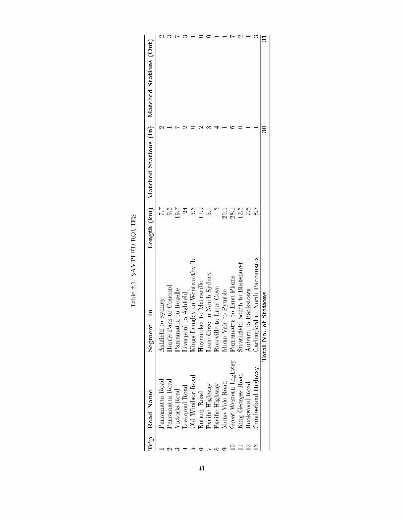
Table2.1:

SAMPLEDROUTES

Trip

RoadName

Segment-In

Length

(km)

MatchedStations(In)

MatchedStations(O

ut)

1Parramatta

Road

Ash�eld

toSydn

ey7.7

22

2Parramatta

Road

HarrisParkto

Concord

9.5

13

3VictoriaRoad

Parramatta

toRozelle

19.7

77

4LiverpoolRoad

Liverpoolto

Ash�eld

242

35

Old

Windsor

Road

Kings

Langley

toWentworthville

5.3

01

6BotanyRoad

Haymarketto

Matraville

11.9

20

7Paci�cHighw

ayLaneCoveto

North

Sydn

ey5.1

30

8Paci�cHighw

ayRosevilleto

LaneCove

34

19

MonaValeRoad

MonaValeto

Pym

ble

20.1

11

10Great

Western

Highw

ayParramatta

toEmuPlains

28.1

67

11KingGeorges

Road

Strath�eld

Southto

Blakehurst

12.5

02

12Rookw

oodRoad

Aub

urnto

Bankstown

7.5

11

13Cum

berland

Highw

ayCarlin

gfordto

North

Parramatta

6.7

13

TotalNo.ofStations

30

31

41

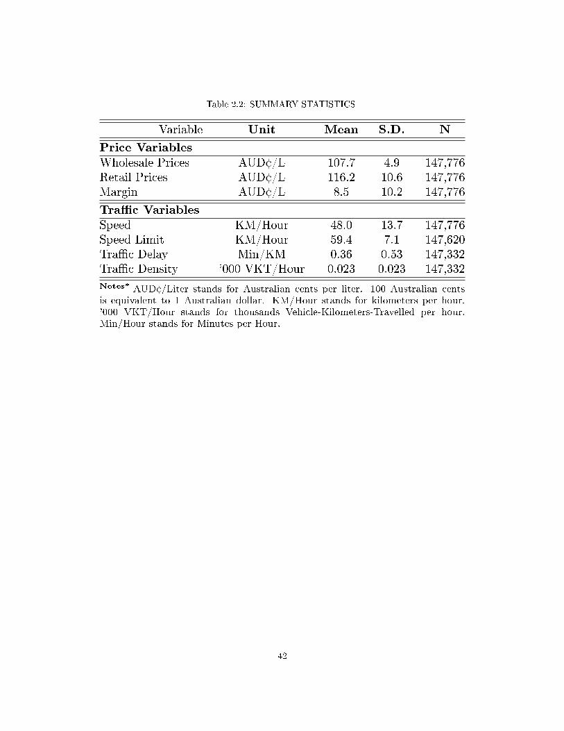
Table 2.2: SUMMARY STATISTICS

Variable Unit Mean S.D. N

Price VariablesWholesale Prices AUD¢/L 107.7 4.9 147,776Retail Prices AUD¢/L 116.2 10.6 147,776Margin AUD¢/L 8.5 10.2 147,776

Tra�c VariablesSpeed KM/Hour 48.0 13.7 147,776Speed Limit KM/Hour 59.4 7.1 147,620Tra�c Delay Min/KM 0.36 0.53 147,332Tra�c Density '000 VKT/Hour 0.023 0.023 147,332Notes* AUD¢/Liter stands for Australian cents per liter. 100 Australian centsis equivalent to 1 Australian dollar. KM/Hour stands for kilometers per hour.'000 VKT/Hour stands for thousands Vehicle-Kilometers-Travelled per hour.Min/Hour stands for Minutes per Hour.

42

Table 2.3: EFFECT OF TRAFFIC CONGESTION ON MARGINS

Dependent variable: Marginijt

(1) (2) (3) (4)All observations No speeding tra�c Workdays No speeding tra�c & workdays

Tra�c Delay 0.290** 0.268** 0.328** 0.315**(0.127) (0.123) (0.141) (0.141)

No. of Stations within 5 KM 0.0651 0.399 0.294 0.622(0.245) (0.394) (0.634) (0.713)

Tra�c Density -3.998 -6.716** -1.340 -1.781(2.590) (3.204) (3.277) (4.133)

Rainfall -0.0551 -0.0291 -0.102* -0.0670(0.0433) (0.0370) (0.0601) (0.0467)

Tra�c Delay (1 day prior) 0.0247 -0.00235 -0.00593 -0.0696(0.0657) (0.0621) (0.111) (0.105)

Tra�c Delay (2 days prior) 0.0484 -0.00122 0.0263 -0.0245(0.0766) (0.0742) (0.110) (0.105)

Tra�c Delay (3 days prior) -0.127* -0.0893 -0.109 -0.0654(0.0712) (0.0655) (0.108) (0.102)

Tra�c Delay (1 week prior) 0.0254 0.0180 0.0172 0.00493(0.155) (0.149) (0.157) (0.152)

Tra�c Delay (2 weeks prior) -0.236* -0.189 -0.199 -0.151(0.131) (0.131) (0.134) (0.132)

Constant 9.512*** 7.954*** 7.452** 5.890(1.265) (1.972) (3.296) (3.610)

Station FE× Month FE Yes Yes Yes YesDate FE Yes Yes Yes YesHour-of-Day FE Yes Yes Yes YesMean margins (AUD¢/liter) 8.54 8.38 7.94 7.79E�ect as percentage of the mean 3.4% 3.2% 4.1% 4.0%N 107,791 92,164 75,396 64,305R2 0.800 0.803 0.778 0.784Notes* The dependent variable in all regressions is the retail margin of regular gasoline measured in Australian cents per litre. Standard errorsare clustered two-way at station i and the route j level.*** p<0.01, ** p<0.05, * p<0.1

43

Table 2.4: EFFECTS ON DIFFERENT TYPES OF GASOLINE


(1) (2) (3)Gasoline type Regular Mid-grade PremiumTra�c Delay 0.315** 0.123 0.179

(0.141) (0.135) (0.129)N 64,305 63,335 81,173R2 0.784 0.820 0.823Notes* The dependent variable in all regressions is marginit,measured in Australian cents per litre. Speci�cation in allcolumns replicate that of column 4 of table 3. Standard errorsare clustered two-way at station i and the route j level.*** p<0.01, ** p<0.05, * p<0.1

44

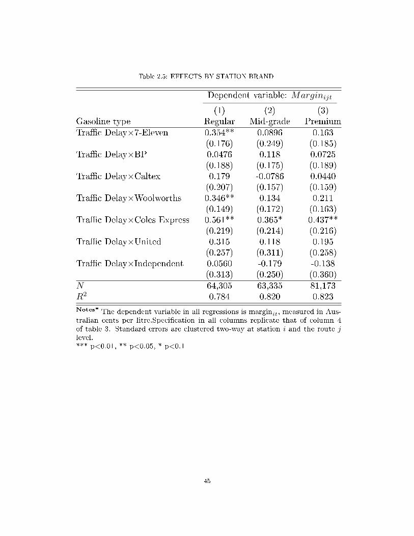
Table 2.5: EFFECTS BY STATION BRAND


(1) (2) (3)Gasoline type Regular Mid-grade PremiumTra�c Delay×7-Eleven 0.354** 0.0896 0.163

(0.176) (0.249) (0.185)Tra�c Delay×BP 0.0476 0.118 0.0725

(0.188) (0.175) (0.189)Tra�c Delay×Caltex 0.179 -0.0786 0.0440

(0.207) (0.157) (0.159)Tra�c Delay×Woolworths 0.346** 0.134 0.211

(0.149) (0.172) (0.163)Tra�c Delay×Coles Express 0.561** 0.365* 0.437**

(0.219) (0.214) (0.216)Tra�c Delay×United 0.315 0.118 0.195

(0.257) (0.311) (0.258)Tra�c Delay×Independent 0.0560 -0.179 -0.138

(0.313) (0.250) (0.360)N 64,305 63,335 81,173R2 0.784 0.820 0.823Notes* The dependent variable in all regressions is marginit, measured in Aus-tralian cents per litre.Speci�cation in all columns replicate that of column 4of table 3. Standard errors are clustered two-way at station i and the route jlevel.*** p<0.01, ** p<0.05, * p<0.1

45

Chapter 3

Is the E�ect of Consumer Search Cost on Price

Dispersion Non-monotonic? Evidence from the

Retail Gasoline Industry

A theme in the consumer search literature is to understand the implications of consumer

search behavior for market outcomes. In his seminal paper �Information of Economics�,

Stigler (1961) claims that price dispersion is a manifestation of ignorance in the market.

The intuition is that some �rms can charge higher prices than others to exploit uninformed

consumers in the market. In consumer search models, search cost avoidance is used to ratio-

nalize why some consumers decide against searching thus choosing ignorance over knowledge.

Succinctly, consumer search literature posits that observed price dispersion for homogeneous

goods can be attributed to the presence of consumer search cost in the market.

However, there is a dearth of research papers that empirically investigate the e�ect of

search cost on price dispersion. This can be attributed at least three empirical di�culties.

The �rst di�culty is that search cost is generally observable. One solution in the literature

is the use of a proxy variable for search cost.1 A popular proxy in the literature is to

1The alternative method is to structurally estimate search cost from price data. See, for example, Hong

46

compare the level of price dispersion between online and o�ine markets. The idea behind

this approach is that online search cost is lower (entails mouse clicks) compared to searching

o�ine (entails traveling to stores). However, research by Ellison and Fisher Ellison (2005)

and Ellison and Ellison (2009) has raised concern that online and o�ine search cost may

not be directly comparable since online sellers can employ new obfuscation strategies such

as �bait-and-switch� that are unavailable to sellers in o�ine markets.

Another well-known issue is the non-monotonic relationship between equilibrium price

dispersion and search intensity. This issue is highlighted in Chandra and Tappata (2011)

who use a version of consumer search model to show that equilibrium price dispersion has an

inverse-U relationship with search intensity. Brown and Goolsbee (2002) and Pennerstorfer

et al. (Forthcoming) provide empirical evidence for this relationship in life insurance and

retail gasoline market respectively. The non-monotonic relationship between equilibrium

price dispersion and search intensity implies that the relationship between equilibrium price

dispersion and search cost may also be non-monotonic and especially when search intensity

is linearly dependent on search cost. Consequently, establishing the empirical relationship

between equilibrium price dispersion and search cost requires researchers to accommodate

non-monotonicity between the two variables.

This paper aims to establish the global relationship search cost on equilibrium price

dispersion in the context of retail gasoline market. My empirical strategy for identifying

the e�ect of search cost in this market relies on the variation in tra�c congestion. The

rational for this approach is based on two empirical facts. The �rst fact is established by

transport engineering literature that travel time and gasoline consumed both increase when

tra�c �ow is obstructed2. The second is established by Castilla and Haab (2013) who �nd

that the majority of consumers who search for cheaper gasoline do so while they drive and

their search cost is a function of the amount of gasoline consumed while driving and the

time spent searching for prices. Together, these two empirical facts imply that search cost

for consumers in the retail gasoline market is always increasing in the severity of tra�c

congestion.

and Shum (2006).2c.f. Tobin (1979) and Jereb, Kumper²£ak, and Bratina (2018)

47

My empirical analysis uses high-frequency tra�c and gasoline price data from Sydney,

New South Wales (NSW). The tra�c dataset is collected by Road and Maritime Services

(RMS)3 and in which I observe hourly tra�c speed and tra�c volume for 36 road segments

in Sydney over a 3-month period from 1 August to 31 October 2016. The price data for the

same period is collected by NSW Fair Trading4

There are several advantages with using this data set to identify the empirical e�ect

of search cost on price dispersion. The �rst one is its high-frequency nature which allows

for the exploitation of intraday variation in tra�c congestion. Tra�c congestion can vary

both spatially and temporally. In an urban setting, tra�c congestion for the same location

can vary signi�cantly within a day due to commuter tra�c and the occurrence of tra�c

accidents. The hourly frequency of my data allows me to exploit these intraday variations

in tra�c congestion. Second, because I observe both the actual tra�c speed and the free-�ow

tra�c speed de�ned by the legal speed limit, I am able to quantify tra�c congestion as travel

time delay in tra�c, or more succinctly, tra�c delay which is a continuous variable. This

continuous measure allows me to test for a variety of non-monotonic relationship between

search cost in tra�c and equilibrium price dispersion between gas stations. In addition, the

panel nature of the data allows me to control for unobserved e�ects across space and time

with �xed e�ects. Finally, my price data includes the complete history of prices for every

sampled gas stations which means that the sampling concern described in Lewis (2008) and

Pennerstorfer et al. (Forthcoming) is not an issue in this paper. 5

I preface my empirical analysis with a conceptual framework based on the consumer

search model presented in Chandra and Tappata (2011). With this conceptual framework,

I show that search cost and equilibrium price dispersion follows an inverse-U relationship.

Using price data for regular gasoline, my empirical results suggest that the impact of tra�c

congestion on equilibrium price dispersion is indeed not monotonic. Speci�cally, I �nd that

the e�ect is inverse-U shaped: for low levels of tra�c delay, equilibrium price dispersion is

3The state road transport authority.4A state government division for regulating retail business practices5Lewis (2008) relies on price data reported by roaming spotters and Pennerstorfer et al. (Forthcoming)

relies on random sampling by the Austrian government: data in both studies are subject to omission of pricedata from one or more stations in a local market.

48

increasing in tra�c delay and for high levels of tra�c delay, equilibrium price dispersion

is decreasing in tra�c delay. The turning-point of this relationship is at 1.39 minute per

kilometer in terms of tra�c delay or 42% of the average legal speed limit in my sample.

This result is robust to alternative de�nitions of price dispersion, the inclusion of high-

frequency time �xed e�ects, correcting standard errors for spatial and serial correlations, and

alternative de�nitions of local markets. However, the e�ect of tra�c delay on equilibrium

price dispersion di�er across gasoline types. For mid-grade gasoline, the result is at best

inconclusive: price dispersion appears to be monotonically increasing in tra�c delay in one

measure of price dispersion but inverse U-shaped for others. For premium-grade gasoline,

the estimates are all statistically indistinguishable from zero.

3.1 Related literature

Within the large empirical literature that links price dispersion to consumer search behav-

ior6, this paper is related speci�cally to the literature that investigates how price dispersion

responds to the �cost� of search, which has largely relied on comparing price dispersion be-

tween online and o�ine prices in a variety of consumer markets7. For o�ine-only markets,

the idea that tra�c quality between �rms may a�ect spatial search cost has been discussed

in Sherman and Weiss (2017) who use di�erent days of the week to examines the e�ect

of pedestrian tra�c on price di�erences between outdoor grocery sellers. This paper con-

tributes towards this literature by relying actual observations of tra�c congestion to study

the e�ect of consumer search cost on equilibrium price dispersion in an o�ine-only market.

This paper is also related to the literature that empirically investigates the non-monotonic

relationship between equilibrium price dispersion and search. Brown and Goolsbee (2002)

�nd that price dispersion in the life insurance market follows a cubic-relationship to the

share of internet users in the population. They proxy search intensity with the ratio of the

number of consumers with low search cost (internet users) to the total number of consumers

6Baye, Morgan, Scholten, et al. (2006) provides an excellent review of this literature.7(c.f. Brynjolfsson and Smith (2000), Clay, Krishnan, and Wol� (2001), Ancarani and Shankar (2004),

Degeratu, Rangaswamy, and Wu (2000) , Orlov (2011) and Sengupta and Wiggins (2012) )

49

in the market. Also employing a ratio of consumer numbers as a proxy for search intensity

is Pennerstorfer et al. (Forthcoming) who �nd that equilibrium price dispersion in the retail

gasoline market has an inverse U-shaped relationship with the share of informed consumers

(long-distance commuters) in the retail gasoline market.8

Finally, this paper is related to the literature that examines the determinants of equilib-

rium price dispersion in the retail gasoline market. Other determinants that have already

been examined include the number of rivals (Barron, Taylor, and Umbeck (2004) and Lewis

(2008)), waiting time at the station (Png and Reitman (1994)), price transparency (Luco

(2019)) and informedness of consumers (Pennerstorfer et al. (Forthcoming)). In summary,

to the best my knowledge, this paper is the �rst to establish the global relationship between

equilibrium price dispersion and search cost in the retail gasoline market.

The remainder of the paper is organized as follows. Section 3.1 presents the related lit-

erature. Section 3.2 presents a modi�ed version of the a consumer search model to illustrate

the predicted relationship between search cost and price dispersion. Section 3.3 describes

the data and the construction of key variables. Section 3.4 describes the empirical strategy

and the results. Section 3.6 provides robustness tests. Section 3.7 concludes.

3.2 Tra�c congestion and consumer search cost - a con-

ceptual framework

Search cost is de�ned in Baye, Morgan, Scholten, et al. (2006) to be consist of �consumers'

opportunity cost of time in searching for lower prices plus other costs associated with ob-

taining price quotes from competing �rms�. This de�nition implies that, holding everything

else �xed, the search cost will be higher in the market if all consumers have to spend more

time for their search. In the context of retail gasoline market, Castilla and Haab (2013)

�nd that 75% of gasoline consumers search while they drive and this �nding allows them to

8Pennerstorfer et al. (Forthcoming) argue that compared to short-distance commuters de�ned as com-muters who live and work within the local market, long-distance commuters de�ned as commuters whotravel beyond the the boundary of at least one local market for work, are better informed because they cansample price from more stations during their commute.

50

conclude that search cost in this market should be a function of the time spent on searching

in tra�c. Since travel time in tra�c is dependent on tra�c condition, the search cost over

the same distance of road will therefore be higher when tra�c is congested. stations.9.

I use a modi�ed version of the consumer search model in Chandra and Tappata (2011) to

illustrate how equilibrium price dispersion will respond to tra�c congestion. In their model,

the equilibrium search intensity in the market is determined by the share of informed con-

sumers called �shoppers� (consumers with zero search cost) and the level of search cost facing

nonshoppers (uninformed consumers who must incur search cost to obtain information) in

the market. In the context of retail gasoline market, shoppers can be considered as con-

sumers who search online while nonshoppers are consumers who search while they drive. I

modify their modeling assumption on the propensity to search for nonshoppers (consumers

with positive search cost) to better suit the context of the retail gasoline market. Speci�-

cally, I model the realization of search cost in the market as a random and common draw

to all consumers but each consumer has di�ering indi�erence level. The common draw as-

sumption is to suit the empirical reality that tra�c congestion increases the travel time for

all drivers on the same road at the same rate. The indi�erence level re�ects the maximum

amount of time a consumer is willing to spend for searching, which is decreasing in the valu-

ation of time by individual consumers. This modi�cation re�ects the empirical observation

that consumers searching within a local spatial market experience similar increase in the

time spent on search due to tra�c congestion but their search decisions depend on their

individual opportunity cost of time.

3.2.1 The Model

Assume a homogeneous-good market with n �rms engage in price competition and have

the same constant marginal cost of c. There is a unit mass of consumers with inelastic

demands and common valuation of v. A fraction of λ consumers are �shoppers�. The

remaining consumers are nonshoppers who decide between remaining ignorant or engage in

9Reduce tra�c �ow as a result of tra�c congestion is known to cause additional fuel consumption perdistance traveled. c.f. Tobin (1979) and Jereb, Kumper²£ak, and Bratina (2018)

51

costly search to know all prices in the market. To search, each nonshopper need to incur

a positive, common and exogenous search cost s. Each nonshopper however di�ers in their

indi�erence level ωi so that a nonshopper i searches only if ωi ≥ s. Nonshoppers draw their

indi�erence level from a continuous distribution G (ωi) with ωi ∈ [0, ω]. The total number

of informed consumers in the market is the sum of shoppers and nonshoppers who search.

Denoting the fraction of informed consumers in the market as µ, the equilibrium fraction

of informed consumers in the market can be expressed as µ = λ+ (1−G (s)) (1− λ). This

de�nition of µ also helps distinguish this paper from Pennerstorfer et al. (Forthcoming).

This paper aims to identify the empirical relationship between price dispersion and s while

the goal of Pennerstorfer et al. (Forthcoming) is to identify the equilibrium relationship

between price dispersion and µ through the variation of a proxy for λ.

Varian (1980) shows that, for a given µ, there is a unique Nash Equilibrium in which

�rms play mixed strategies. In each period, �rms simultaneously draw prices from

F (p;µ, c, v, n) = 1−[

(1− µ)

µn

(v − p)(p− c)

]1/(n−1)

where p ∈[p∗ = cnµ+(1−µ)v

1+(n−1)µ , v].

Price dispersion as Gains from Search associated with equation (1) can be written as

GS = E [p− pmin | µ; c, v, n] =

∫ v

p∗p[1− n [1− F (p;µ, c, v, n)]

n−1]dF (3.1)

Using numerical integration, Chandra and Tappata (2011) shows that the non-monotonic

relationship between µ and GS has an inverse-U shape. Given the monotonic relationship

assumed between s and µ, it is straightforward to see that s should follow an inverse-U

relationship with GS. Following Chandra and Tappata (2011), I plot the corresponding

values between s and GS in �gure 3.1 which con�rms the inverse-U relationship: price

dispersion �rst increases in search cost s from 0 to s and then decreases in s from s to 1. 10.

10The parameter values used are n = 5,λ = 0, v = 2, c = 0, G (s)=Is (2, 2), where Is is a beta cumulativedistribution function.

52

3.3 Data and Descriptive Evidence

3.3.1 Tra�c data

Central to my empirical strategy is the assumption that search cost in the retail gasoline

market increases in tra�c congestion. Tra�c delay refers to the extra travel time drivers

experience during their journey as a result of slower than normal tra�c �ow. In the same

spirit of Chandra and Tappata (2011) , the validity of this proxy exploits the fact that

search cost is higher for stations located further away11. Because consumers typically drive

in tra�c to access gasoline stations, for them, the temporal distance between stations will

vary depend on local tra�c condition. The time-varying nature of tra�c condition implies

that for consumers who search while they drive will face higher search cost when the local

road network is experiencing greater levels of tra�c delay.

Until mid-2017, the RMS Roads Report provided hourly observations of tra�c speed

and tra�c density for 60 trips in NSW. 12.

An example of how information is presented in the RMS Roads Report is shown in

�gure (3.2). For each trip, Roads Report provides its description in words, its location on

the map, direction and tra�c observations. Using a web data scraper, I collected a sample

of three months from August to October 2016 for all trips with hourly tra�c speed and

tra�c density observations in the Roads Report.

3.3.2 Measuring tra�c congestion

I follow Anderson (2014) and measure the intensity of tra�c congestion in terms of tra�c

delay

TrafficDelayjt =FreeflowSpeedjActualSpeedjt

− 1 (3.2)

where FreeflowSpeedj is the legal speed limit13 of trip j and ActualSpeedjt is the observed

average tra�c speed for road segment j at time t. For example, an observed speed of 30

11Chandra and Tappata (2011) assumes that search is free between stations that are located immediatelynext to each other (in the same corner); search is costly if otherwise.

12A trip is de�ned in the Roads Report represents a direction-speci�c subsection of a major road.13Reported in the Roads Report by RMS

53

kilometer per hour (kmh) on a trip with a free-�ow speed of 60 kmh corresponds to a tra�c

delay of 1 minute per kilometer (Min/KM).

3.3.3 Price data

The price data is collected by NSW Fair Trading via a government-developed price com-

parison online tool called FuelCheck. FuelCheck contains the full history of station-level

prices for every fuel type sold in the state of NSW from August 2016. My main analysis

focus on the price of regular gasoline (U91) which is the most commonly available gasoline

in Australia. Since 2013, all gas stations in NSW have been required by law to display

the price of their top two selling fuel on a price board visible to the passing drivers. In

2016, U91 accounted for approximately 30% of gasoline sales in NSW making it a top seller

(Australia (2018)). The popularity of U91 means that its price is more likely to be displayed

on price boards making it easier, and hence more probable, for consumers to compare its

price between stations while driving than other gasoline varieties.

An advantage of the FuelCheck data is its high quality in terms of timeliness and accuracy

thanks to the legal requirement that all gas stations must report new prices to FuelCheck

as soon as they change their in-stone prices. Consumers can report mismatches between

online price and in-store price directly via the FuelCheck mobile app and �nes are issued to

non-compliant stations.

FuelCheck also provides the geographic information of each gas station which allows me

to spatially match gas stations to tra�c data. Retail prices are nominal and measured in

Australian cents per liter. Because prices in my sample exhibit little within-hour varia-

tion, my empirical approach examines how equilibrium price dispersion responds to tra�c

congestion at the hourly level.

3.3.4 Measuring price dispersion

I now describe how I construct measures of price dispersion, my outcome of interest. Below

I explain how I de�ne local markets, construct �residual� prices, and the various measures

of price dispersion employed.

54

Local markets

In order to construct measures of equilibrium price dispersion, local markets must �rst be

de�ned. Barron, Taylor, and Umbeck (2004) and Lewis (2008) propose that competition in

the retail gasoline market is mostly local so that a local market should only include direct

competitors that are located closely to each other. A simple method of market delineation

based on this argument involves assigning stations to local market i if they are located

within an euclidean distance to station i. Alternatively, the literature has also identi�ed

local gasoline market by subsections of the road network. For example, Haining (1983)

provides theoretical argument and empirical evidence that price interaction between gasoline

stations are de�ned by principal roadways. Cooper and Jones (2007) also de�ne local spatial

markets by commuting route to study pricing pattern for gasoline. Houde (2012a) argues

that competition among stations may not be solely localized since consumers can substitute

between stations far away from each other but close to a common commuting path. In

addition, Houde (2012a) suggests that spatial market de�nition should be related to the

road network and the direction of the tra�c �ow.

According to the RMS Roads Report, each trip in the report represents a section of a

major communing route in NSW. Based on this description, I follow Houde (2012a) and

de�ne a local market to include all stations located immediately on the left hand side of a

trip. Because each trip represents a single direction of a road, this de�nition of local markets

assumes that stations located on opposite sides of the same road compete in separate local

markets. Figure 3.3 illustrates the stations (black dots) in two local markets: 6 stations

in the local market de�ned by the trip of Pennant Hills Road (Carlingford to Wahroonga)

and 2 stations in the local market de�ned by the trip of Pennant Hills Road (Wahroonga to

Carlingford).

Residual prices

Even though automobile fuel is homogeneous in terms of its physical characteristics, gas

stations di�er not only in their location, but also in terms of services provided and other

characteristics. Thus, a simple explanation for the observed existence of price dispersion

55

relies on station heterogeneity. The challenge is to obtain a measure of price dispersion after

removing the main source of heterogeneity. I follow the literature14 and obtain the residuals

of a price equation and interpret these residuals as the price of a homogeneous product. To

obtain �cleaned� prices I exploit the panel nature of my data following Lach (2002) and run

a two-way �xed e�ects panel regression of �raw� fuel prices (prit) using seller (ζi) and time

(χt) �xed e�ects:

prit = α+ ζi + χt + uit (3.3)

I focus on the residual variation, interpret the residual price pit ≡ uit as the price of a ho-

mogeneous product after controlling for time-invariant store speci�c e�ects and �uctuations

in price common to all stores.

Measures of price dispersion

To examine the impact of search cost on price dispersion I need to summarize the price

distribution in a (local) market as a single metric. Several measures of price dispersion have

been proposed in the literature. I will �rst focus on the �Gains from Search� (GS, also known

as �value of information�). This is a commonly used measure and the testable prediction in

section 3.2 is also based on this metric. The measure has a very intuitive interpretation:

it corresponds to a consumer's expected bene�t of being informed. The GS is de�ned as

the di�erence between the expected price and the lowest expected price in the market. If

the local market assigned to road segment j is de�ned by mj , then the GS for local market

j at time t is given by GSjt = E [pmjt ] − E[pmjt

min

]. I follow Chandra and Tappata (2011)

and use the average local market price pmjt as the estimate for E [pmjt ] while the estimate

of E[pmjt

min

]is given by pmjt

(1) (i.e. the �rst order statistic of prices sampled in market mj).

Subsequently, price dispersion measured as GS in market mj at time t is given by equation

3.4:

GSjt = pmjt − pmjt

min (3.4)

14See e.g. Sorensen (2000), Brown and Goolsbee (2002), Lewis (2008), Chandra and Tappata (2011) orLuco (2019)

56

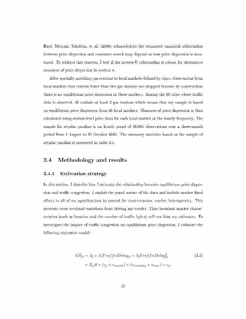
Baye, Morgan, Scholten, et al. (2006) acknowledges the estimated empirical relationship

between price dispersion and consumer search may depend on how price dispersion is mea-

sured. To address this concern, I test if the inverse-U relationship is robust for alternative

measures of price dispersion in section 4.

After spatially matching gas stations to local markets de�ned by trips, observations from

local markets that contain fewer than two gas stations are dropped because by construction

there is no equilibrium price dispersion in these markets. Among the 60 trips where tra�c

data is observed, 36 contain at least 2 gas stations which means that my sample is based

on equilibrium price dispersion from 36 local markets. Measures of price dispersion is then

calculated using station-level price data for each local market at the hourly frequency. The

sample for regular gasoline is an hourly panel of 46,085 observations over a three-month

period from 1 August to 31 October 2016. The summary statistics based on the sample of

regular gasoline is presented in table 3.1.

3.4 Methodology and results

3.4.1 Estimation strategy

In this section, I describe how I estimate the relationship between equilibrium price disper-

sion and tra�c congestion. I exploit the panel nature of the data and include market �xed

e�ects in all of my speci�cations to control for time-invariant market heterogeneity. This

prevents cross-sectional variations from driving my results. Time-invariant market charac-

teristics (such as location and the number of tra�c lights) will not bias my estimates. To

investigate the impact of tra�c congestion on equilibrium price dispersion, I estimate the

following regression model:

GSjt = β0 + β1TrafficDelayjt + β2TrafficDelay2jt (3.5)

+Xjtθ + (γj × τmonth) + (τworkday × τhour) + εjt

57

where j indexes local market and t indexes time; GSjt is a Gains from Search measure of

price dispersion de�ned in equation 3.4; Delayjt is the observed tra�c congestion de�ned by

3.2; Xjt is a vector of control variables including a quadratic function of contemporaneous

tra�c density, a quadratic function of the number of active competing stations in the local

market and the average wholesale gasoline cost; γj × τmonth are interactive �xed e�ects

between market and monthly �xed e�ects; τworkday × τhour are interactive �xed e�ects

between workday �xed e�ects15 and hour-of-the-day �xed e�ects.

Tra�c density measures the number of vehicles passing through a trip within an hour.

Controlling for tra�c density is necessary for isolating the travel time e�ect of tra�c con-

gestion on price dispersion. Tra�c density is correlated with tra�c delay because the �ow

of tra�c is slowed when the capacity of the road is reached. Through its impact on demand

for travel, the price of gasoline is also know to in�uence tra�c density (Burger and Ka�ne

(2009)). Tra�c density is therefore included as a control to address the concern that gasoline

price and tra�c delay may be simultaneously determined. The number of active competing

stations is included as a control because gas stations may have di�erent business hours so

that equilibrium price dispersion may be simply driven by the number of prices available in

the market. Finally, the daily state-wide average of wholesale gasoline price is included as

a control for the e�ect of daily common cost shocks on equilibrium price dispersion.

In the preferred speci�cation, I include γj × τmonth to provide additional control for

unobserved month-to-month variation in market heterogeneity such as local income and

unemployment rate. Finally, τworkday × τhour are included to control for repeating within-

day tra�c cycles for both workdays and non-workdays (weekends and public holidays).

The empirical model, equation (3.5) implies that when the relationship between tra�c

congestion and equilibrium price dispersion is non-monotonic, the estimate of β1 and β2

should be signi�cantly di�erent from zero. The null hypotheses to be tested are H0 : β1 = 0

and H0 : β2 = 0 and the alternative hypotheses are H1 : β1 6= 0 and H1 : β2 6= 0. In

addition, if consumer search cost in the retail gasoline market is indeed increasing in tra�c

congestion then consumer search model in section 3.2 implies that the equilibrium price

15A workday is a day that is not a Saturday, a Sunday or a public holiday.

58

dispersion in my sample should have an inverse-U relationship with tra�c congestion. An

inverse-U relationship can be inferred from a signi�cantly positive estimate of β1 and a

signi�cantly negative estimate of β2.

For robust inference, I cluster the standard errors of my regressions at the local market

level. Furthermore, to address the concern that clustering standard errors might lead to

incorrect inference when cluster size is small, I implement the six-point bootstrap-weight

distribution approach proposed by Webb (2014).

3.5 Estimation results

Panel A of table 3.2 displays the estimated coe�cients for equation 3.5 based on the GS

measure of price dispersion. Column 1 only includes the local market �xed e�ects. Column

2 adds tra�c density, wholesale gasoline price and the number of active local competitors

as covariates to column 1. Column 3 allows for month-speci�c local market �xed e�ects.

Column 4 adds day-type-speci�c hour �xed e�ects to the speci�cation in column 3. Column

4 is my preferred speci�cation. In all four speci�cations, β1 and β2 are statistically signi�cant

at the 10% level which implies the presence of a non-monotonic relationship between GS and

TrafficDelay. The signs of the coe�cient estimates of β1 and β2 in table 3.2 are consistent

with a relationship that has an inverse-U shape. Based on the coe�cient estimates in my

preferred speci�cation, I plot the net relationship between the predicted GS and tra�c delay

in �gure 3.4. Figure 3.4 shows that GS increases with tra�c delay when tra�c delay is low

and decreases with tra�c delay when tra�c delay is high. The corresponding marginal

e�ect of TrafficDelay on GS is therefore 0.280− 0.199Delay.

An additional check of the inverse-U relationship is to ensure that the estimated turning

point − β1

2β2falls within the sample range of TrafficDelay. Panel B of table 3.2 reports that,

based on the 95% con�dence interval derived using the Fieller method16, estimated turning-

points based on all speci�cations in table 3.2 fall within the sample range of TrafficDelay,

con�rming the inverse-U shaped relationship between price dispersion and tra�c delay.

16According to Lye and Hirschberg (2012), the con�dence intervals derived based on the Fieller methodis less susceptible to bias than the delta method.

59

Based on the estimates in column 4, the following can be inferred: 1) a local market displays

the highest level of price dispersion when tra�c delay is about 1.40 Min/KM, 2) the average

level of tra�c congestion has a positive e�ect on equilibrium price dispersion, and 3) the

turning-point value of tra�c delay represents the 94th percentile of tra�c delay observations

in my sample.

3.5.1 Non-parametric evidence of the inverse-U relationship

A possible concern for the inverse-U shaped relationship implied by the coe�cients estimates

on TrafficDelay in table 3.2 is driven by the quadratic function of Delay in the regression

model. To address this concern, I follow Chetty, Friedman, and Rocko� (2014) and use a

binned scatterplot17 to visualize the relationship between GS and TrafficDelay. Figure

3.5 is a binned scatterplot with the residuals from the following regression equation on the

vertical axis and TrafficDelay on horizontal axis.

GSjt = β0 +Xjtθ + (γj × τmonth) + (τworkday × τhour) + εjt (3.6)

The variation in the residuals from equation 3.6 represents the residual variation in

GS after controlling for the covariates and �xed e�ects in 3.5. The rational behind this

approach is that if the inverse-U relationship is not driven by the quadratic speci�cation of

TrafficDelay in 3.5, then binned scatterplot should present corroborating visual evidence

for this relationship between the residual variation from equation 3.6 and TrafficDelay.

Reassuringly, the inverse-U relationship is clearly visible in the binned scatterplot shown in

�gure 3.5. It shows that for the majority of time, price dispersion measured as GS increases

with tra�c delay while the downward portion in the inverse-U relationship is associated

very high levels of tra�c delay greater than 2 Min/Km. It is therefore a concern that the

inverse-U shape is driven by outliers that are potentially measurement errors.

My sample contains some of the most congested roads in Sydney (e.g, Paci�c Highway

17Binned scatter plot is a convenient non-parametric way to identify relationship between two variables inlarge panel datasets such as the one in this paper. It �rst divides the sample into equal sized bins based onobservations of the explanatory variable. Each dot on a binned scatterplot represents the mean of outcomevariable in each bin and the corresponding mean of the the explanatory variable in the same bin.

60

and Alison Road) and it is therefore unsurprising extreme delays are found in my sample.

In fact, drivers on these roads frequently experience delays greater than 4 Min/KM during

commuting peak hours. Extreme tra�c congestion are chronic and common in Sydney as

they have been repeatedly reported in the press (For example, O'Rourke (2014)). Never-

theless, as a robustness check in section 3.6, I drop the top and bottom 1% of observations

based on tra�c delay and show that the inverse-U shaped relationship is not dependent on

presence of outliers.

3.5.2 Mechanism - opportunity cost of time

The result so far suggests that the relationship between equilibrium price dispersion in the

retail gasoline market and tra�c congestion is consistent with the relationship between

equilibrium price dispersion and consumer search cost implied by my conceptual model. In

this section, I test the assumption that the opportunity cost of time is one of the channels

through which tra�c congestion a�ects consumer search cost in the the retail gasoline mar-

ket. Following Chandra and Tappata (2011), I do this by estimating the e�ect of tra�c

congestion on equilibrium price dispersion of mid-grade gasoline (P95) and premium gaso-

line (P98). Chandra and Tappata (2011) postulate that consumer search cost increases in

the grade of gasoline. This association is based on the assumption that, on average, con-

sumers of a higher grade of gasoline are wealthier and hence have higher opportunity cost

for their time.

Assuming there is no cross-grade substitution, consumer types can be modeled as having

grade-speci�c distribution of indi�erence level Gh (ωi) where h ∈ {U91,P95,P98}. Because

indi�erence level represents the maximum amount of time a consumer is willing to spent

on searching, a higher opportunity cost will imply a lower indi�erence level. An increase

in opportunity cost therefore implies a leftward shift of Gh (ωi). In other words, for every

realization of search cost s, the probability of searching decreases in the grade of gasoline.

This implies that the share of consumers who search on the margin is decreasing in the

grade of gasoline. In the extreme case, no consumer will search if the lower bound of their

indi�erence level is su�ciently high. If opportunity cost of time is the indeed the channel

61

through which tra�c congestion a�ects consumer search cost, then for higher grades gasoline,

we should expect price dispersion to be less dependent on tra�c congestion and hence a

�atter relationship between price dispersion and tra�c congestion.

Figure 3.6 plot the net relationship between GS and Delay for regular, mid-grade and

premium gasoline. Figure 3.6 shows that compared to regular gasoline, the inverse U-shape

becomes �atter for mid-grade gasoline and completely �at for premium gasoline. This

pattern is consistent with the explanation that search decision by consumers with higher

opportunity cost is less sensitive to tra�c congestion because fewer of them will spend time

searching in tra�c.

3.6 Robustness tests

In this section, I provide a number of robustness tests for my main result presented in column

4 of table 3.2. Speci�cally, I examine if the inverse-U relationship is robust to alternative

measures of price dispersion, GS constructed from raw instead of cleaned prices and the

removal of outliers from the sample.

3.6.1 Alternative measures of price dispersion

Baye, Morgan, Scholten, et al. (2006)) acknowledges that the estimated empirical relation-

ship between price dispersion and consumer search cost may depend on how price dispersion

is measured. It is therefore possible that the inverse-U relationship may not hold between

tra�c congestion and measures of equilibrium price dispersion other than GS. To address

this concern, I re-estimate equation 3.5 to with alternative measures of equilibrium price

dispersion. The alternative measures considered are standard deviation and interquartile

range which are two common measures of equilibrium price dispersion examined in the gaso-

line pricing literature18. Figure 3.7 plot the net e�ect of tra�c congestion on Gains from

Search, standard deviation and interquartile range. Comparing to the Gains from Search

measure, the inverse-U shape appears more apparent for the interquartile range measure

18c.f. pennerstorfer2017information points out that interquartile range is a better measure for pricedispersion than standard deviation and sample range as it is less susceptible to outliers in the price data.

62

and less apparent for the standard deviation measure. Nevertheless, it can be concluded

from �gure 3.7 that tra�c congestion has an inverse-U relationship with equilibrium price

dispersion measured as Gains from Search, standard deviation and inter interquartile range.

3.6.2 Raw prices

It is possible that the regression model, equation 3.3, for generating residual prices is mis-

speci�ed. To ensure that my results are not driven by this speci�cation error, I re-estimate

my preferred speci�cation with raw prices instead of residual prices. Based on the coe�-

cient estimates from this regression, the implied net relationship between Delay and GS is

presented in �gure 3.8b. When compared to the main result which is reproduced in �gure

3.8a, the relationship shown in �gure 3.8b is �atter but still inverse-U shaped. This di�er-

ence is expected because a larger share of variation in raw price dispersion is explained by

factors other than search cost such as location, branding and service di�erences between gas

stations. In spite of this, �gure 3.8b suggests that the inverse-U relationship is robust to

potential misspeci�cation of equation 3.3.

3.6.3 Dropping extreme tra�c delay

To address the aforementioned concern that the curvature of the relationship is driven by

outliers of extreme tra�c delay, I re-estimate my preferred speci�cation with a subsample

which drops the top and bottom 1% observations of tra�c delay. Compared to the net

relationship in the full sample in �gure 3.9a, �gure 3.9b shows that the curvature of the

inverse-U relationship is reduced after dropping observations associated with extreme tra�c

delay. Visually, the inverse-U relationship appears to survive the removal of extreme values

of tra�c delay. To con�rm this, I formally verify the presence of an inverse-U relationship in

the restricted sample by applying the statistical test in Lind and Mehlum (2010).19 The test

veri�es if the slope of the relationship between TrafficDelay andGS is signi�cantly positive

for low values of TrafficDelay and signi�cantly negative for high values of TrafficDelay.

19Lind and Mehlum (2010) argues that while a positive linear and a negative quadratic term supports aconcave relationship between two variables, it is not su�cient to guarantee an inverse-U shaped relationshipsince the relationship may be concave but still monotone in relevant range.

63

The null hypothesis in this test is that the relationship is either linear or U-shape and the

alternative hypothesis is that the relationship is inverse-U shaped. The test produced a

p-value of 0.0365 which implies that the null is rejected. Based on the visual and statistical

evidence presented, it can be concluded that the inverse-U relationship is robust to dropping

extreme values of tra�c delays.


This paper provides an empirical examination on the global relationship between consumer

search cost and equilibrium price dispersion. Based on a modi�ed version of consumer search

model presented in Chandra and Tappata (2011), I predict that the relationship between

search cost and equilibrium price dispersion is non-monotonic and inverse-U shaped. I

test this prediction in the retail gasoline market by estimating the global e�ect of tra�c

congestion on equilibrium price dispersion observed between gas stations along the same

side of a major road in New South Wales. My empirical strategy exploits the fact that

tra�c congestion can increase consumer search cost in the retail gasoline market.

I �nd that tra�c congestion and equilibrium price dispersion for regular gasoline has

a non-monotonic relationship which is inverse U-shaped. The turning point for this rela-

tionship corresponds to a tra�c delay of 1.40 Min/KM. Equilibrium price dispersion in this

result uses the Gains from Search measure constructed from residual prices after control-

ling for time-invariant station heterogeneity and time-varying common shocks. The same

inverse-U relationship is obtained when equilibrium price dispersion is measured as standard

deviation and interquartile range. Consistent with the income hypothesis by Setiawan and

Sperling (1993), I �nd this relationship is weaker for mid-grade gasoline and insigni�cant

for premium gasoline. These results are consistent with the interpretation that wealthier

consumers are less likely to search in tra�c due to their higher opportunity cost of time.

This paper is the �rst empirically establish a non-monotonic relationship between con-

sumer search cost and equilibrium price dispersion in the retail gasoline market. For future

empirical investigations into the impact of search cost on equilibrium price dispersion in

64

other markets, my �ndings highlight the need to allow for non-monotonic relationship in

their empirical strategies.

My results can also be appreciated by antitrust agencies who monitor the level of price

competition in the retail gasoline market. Following the interpretation of turning-point

location by Chandra and Tappata (2011), my �nding suggests that pricing of regular gasoline

is more consistent with competitive pricing for 94% of the time and more consistent with

monopolistic pricing for 6% of the time. This inference is made based on the fact that the

estimated turning-point value of tra�c delay corresponds to the 94th percentile of all tra�c

delay observations in my sample.

65


Figure 3.1: SEARCH COST (s) AND GAINS FROM SEARCH

66

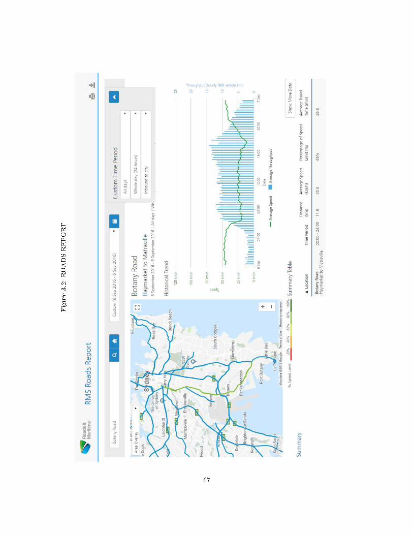
Figure3.2:

ROADSREPORT

67

Figure 3.3: TWO EXAMPLES OF LOCAL MARKET

Note. Gas stations are shown as black dots.

68

Figure 3.4: NET RELATIONSHIP BETWEEN TRAFFIC DELAY AND GAINS FROMSEARCH

Note. This graph is based on the speci�cation of column 4 in table 2. Price dispersion in this diagram isbased on the Gains from Search measure

69

Figure 3.5: BINNED SCATTERPLOT OF of GS ON Delay

Note. The �gure is a binned scatter plot in which observations are organised into 100 equal sized binsand each point in the �gure represents the average of 460 observations. The curve is a quadratic line of best�t

70

Figure3.6:

NETRELATIO

NSH

IPBETWEENTRAFFIC

DELAYANDGAIN

SFROM

SEARCHBYGASO

LIN

ETYPE

(a)Regulargasoline(U

91)

(b)Mid-gradegasoline(P95)

(c)Premium

gasoline(P98)

71

Figure3.7:

ROBUST

NESS

TEST

-ALT

ERNATIV

EMEASU

RESOFPRICEDISPERSION

(a)Gainsfrom

Search(baseline)

(b)Standard

Deviation

(c)InterquartileRange

72

Figure 3.8: ROBUSTNESS TEST - RAW PRICES

(a) Residual prices

(b) Raw prices

73

Figure 3.9: ROBUSTNESS TEST - DROPPING EXTREME TRAFFIC DELAY

(a) Full sample

(b) Sub-sample - dropping outliers of tra�c delay

74

Table3.1:

SUMMARYST

ATISTICS

Variable

Unit

Mean

Std.Dev.

Min.

Max.

Observations.

Pricedata

-ResidualPrices

Average

Price

Cents

per

litre

0.066

5.733

-21.634

24.297

46085

Price

dispersion

Gains

from

Search

Cents

per

liter

2.786

3.732

0.002

24.771

46085

Standard

Deviation

Cents

per

liter

2.72

3.114

0.003

19.005

46085

SampleRange

Cents

per

liter

5.641

6.374

0.005

36.332

46085

Pricedata

-RawPrices

Average

Price

Cents

per

litre

115.466

10.344

93140.45

46085

Price

dispersion

Gains

from

Search

Cents

per

litre

3.111

4.373

027.12

46085

Standard

Deviation

Cents

per

litre

2.997

3.633

020.295

46085

Range

Cents

per

litre

6.107

7.306

037

46085

Tra�cdata

Tra�cSp

eed

Kilometre

per

Hour

47.314

12.674

8.175

8446085

Tra�cVolum

eVehicle-K

ilometres-per-hour

8.721

6.464

0.1

41.45

46085

SpeedLim

itKilometresper

Hour

59.765

6.658

50.513

79.971

46085

Tra�cDelay

Minutes

per

Kilometre

0.387

0.543

-0.117

5.823

46085

Num

ber

ofstations

observed

120

Num

ber

ofMarkets

36Average

Num

ber

ofStations

inaMarket

2.7

75

Table 3.2: NON-MONOTONIC EFFECT OF TRAFFIC CONGESTION ON EQUILIB-RIUM PRICE DISPERSION OF REGULAR GASOLINE

Dependent Variable Gains from Search(1) (2) (3) (4)

Panel ATrafficDelay 0.230** 0.234** 0.258*** 0.255**

(0.0917) (0.102) (0.0934) (0.118)TrafficDelay2 -0.0770*** -0.0790*** -0.0862*** -0.0907***

(0.0247) (0.0267) (0.0248) (0.0320)Wholesale price N Y Y YTra�c density N Y Y YNo. of active station N Y Y YMarket FE Y Y N NMonth-speci�c market FE N N Y YDay-type-speci�c hour FE N N N YPanel B

Turning point (s = −β1

2β2) 1.49 1.48 1.50 1.40

95 percent C.I. of the turning point [0.69,1.92] [0.46,1.89] [0.85,1.83] [-0.086,1.78]N 45,196 45,196 45,196 45,196R2 0.112 0.133 0.192 0.195Notes* This table presents the estimated e�ect of tra�c on price dispersion. The depdendent variable is pricedispersion measured as Gains from Search constructed from residual prices from equation (2). Standard errorsare clustered at the local market level. Inferences in panel A is based on bootstrapped stdandard errors followingthe six-point bootstrap-weight distribution approach proposed by Webb(2014). In Panel B, con�dence intervalsof the turning points are derived using the Fieller method. *** p<0.01, ** p<0.05, * p<0.1

76

Chapter 4

Reference-Dependent Demand, Price Cycle and

Competition in Retail Gasoline Market

4.1 Introduction

Asymmetrical price cycles have been found in retail gasoline markets around the world

including the United States, Canada ,Germany and Australia. While a signi�cant amount

of research has studied this phenomenon, an ongoing research question in the literature

revolves around whether it is an outcome of competitive or cooperative pricing strategy by

gasoline �rms. Answering this question is of particular interest to governments who have

raised concern that gasoline price cycles are collusive in nature (Parliament of Australia

(2006) and Hydro and Pellatt (2006)). Research papers o�ering empirical evidence for

competition such as Eckert (2003), Noel (2007a), Noel (2007b), Atkinson (2009), Lewis

(2009) Wang (2009) and Linder et al. (2018) aim to demonstrate that gasoline price cycles are

a manifestation of the non-cooperative dynamic price equilibrium known as the Edgeworth

Cycle (EC) formalized in Maskin and Tirole (1988). On the other hand, researchers have also

found evidence of tacit collusion in some gasoline markets with price cycles. For example,

in separate markets, gasoline companies are found to coordinate their prices through focal-

77

point in price timing (Foros and Steen (2009)), price leadership by large �rms (Lewis (2012)),

and price experimentation and signaling (Byrne and De Roos (2019)).

This paper contributes towards answering this question by examining whether pricing

behavior under gasoline price cycle is dependent on the price elasticity of demand for gaso-

line. The rational for this test is based on the prediction by Noel (2008) that, under an

EC equilibrium, price cycles are longer when aggregate demand for the good is more price

elastic. The intuition for this prediction is that �rms will, under the EC equilibrium, re-

spond to more elastic demand by lowering their undercutting aggressiveness resulting in a

longer period of time to reach the bottom of a cycle. Hence, this paper attempts to establish

whether gasoline price cycle is consistent with EC through estimating the impact of demand

elasticity on its cycle length and undercutting aggressiveness.

The ideal data for my empirical analysis would include direct observations of demand

elasticity for gasoline or the price and demand data for estimating them. In the absence of

such data, my empirical analysis exploits a proxy variable constructed using only gasoline

price data. This proxy variable measures whether current average gasoline price is higher

or lower than a historical average of past prices. The relevance of this proxy is based on the

idea of reference-dependent demand in behavioral economies which suggests that reference-

dependent demand becomes more price elastic when consumers believe the price they face

is higher than their reference-price: a psychological price threshold. Hence, the validity of

my proxy variable relies heavily on the assumption that demand for gasoline is reference-

dependent. This assumption has been tested by a number of empirical papers including

Lewis and Marvel (2011), Castilla and Haab (2015) and Levin, Lewis, and Wolak (2019).

Findings from these papers are supportive of this assumption, in the sense that, higher

gasoline prices are found induce consumer behavior that can interpreted as having more

price sensitive demand. It is important to note that all conclusions made for the e�ect of

aggregate demand elasticity are therefore inferred from the estimated impact of the proposed

proxy variable.

To preview my results, I �nd that positive deviations from the reference-price increased

the length of gasoline price cycle by 3.5 days (13% of the sample mean). After establishing

78

its impact on cycle length, I then investigate if positive deviation from the reference-price

has any e�ect on undercutting aggressiveness. Using the magnitude of average price cut

from each price cycle as a measure for undercutting aggressiveness, I �nd that positive

deviations from the reference-price decreased undercutting aggressiveness by 0.72 cents per

liter (22% of the sample mean). To control for the impact of wholesale cost of gasoline on

pricing decisions, I also show that positive deviations from the reference-price has a similar

impact on the magnitude of average margin cut. Based on the assumption that demand for

gasoline is reference-dependent, I infer from these results that estimated pricing behavior

under gasoline price cycle in my sample is consistent with predicted pricing behavior under

the EC. Additionally, I show that gas stations of all brands reduced their undercutting

aggressiveness when demand is inferred to be more elastic suggesting that my conclusion is

valid for all gasoline companies in my sample. Finally, I show that my results are robust to

alternative de�nitions of reference-price based on a variety of time horizons of past prices.

The rest of the papers is organized as follows. Section 4.2 describes related literature

and theory to be empirically tested. Section 4.3 describes the data and o�ers descriptive

evidence. Section 4.4 presents the empirical strategy. Section 4.4.2 presents the results.

Section 4.5 concludes.

4.2 Literature and hypotheses

The EC equilibrium formalized by Maskin and Tirole (1988) is widely acknowledged in

the literature as the leading theory that explains the asymmetrical price cycles observed

in the retail gasoline market. In their model, Maskin and Tirole (1988) assume two �rms

are engaged in price competition over a homogeneous product for an in�nite number of

periods1. An EC consists of three phases in the order of Restoration, Undercutting and

War-of-Attrition. The Restoration phase is completed over one period with a large price

increase from the bottom of the previous cycle; the Undercutting phase is comprised of

multiple periods of small price cuts resulting in a graduate decline in price towards the

1One �rm can change its price in each period and the two �rms alternate in setting price every period.They also face �xed demand and have �xed production cost.

79

marginal cost; the cycle ends with the War-of-Attrition phase de�ned by one or several

periods of static price prior to the Restoration phase of the next cycle. Importantly, the

Undercutting phase of an EC is theorized by Maskin and Tirole (1988) to be driven by

a competitive process of �rms taking turns to undercut each other to steal market share.

Consequently, an EC can be interpreted as an outcome of competition.

Previous research (Eckert and West (2004), Noel (2007a), Noel (2007b), and Wang

(2009)) that attempted to establish observed gasoline price cycle as EC has commonly

relied on the implied role of small �rms in generating EC according to Eckert (2003). In

his model, Eckert (2003) shows that EC is more likely to be found in markets that have a

signi�cant di�erence in outlet numbers between two �rms. The intuition for this approach

is that the small �rm (the �rm that has the lower share of outlets in a market) is more likely

to lead price cuts that trigger the Undercutting phase of EC. The empirical implication is

that gasoline price cycle is consistent as EC if it is more likely to be found in markets with

a greater share of small �rms.

In Noel (2008), the author predicts that the shape of EC should respond to aggregate

demand elasticity. Speci�cally, cycle length is expected to increase in the aggregate demand

elasticity. Noel (2008) explains that this is because the speed at which prices fall during the

Undercutting phase decreases if consumers are more price sensitive. The intuition is that

a smaller price cut can now steal the same amount of demand as a larger price cut when

consumers are less price sensitive. Based on this prediction, Isakower and Wang (2014)

use the di�erence in demand elasticity of Lique�ed Petroleum Gas (LPG) and gasoline to

explain the di�erence in their price cycle length.

Due to the lack of gasoline demand data, this paper proposes to infer price elasticity

of demand from price data by assuming that demand for gasoline is reference-dependent.

This assumption has been examined by Lewis and Marvel (2011), Castilla and Haab (2015)

and Levin, Lewis, and Wolak (2019). The contribution of this paper over these papers is on

the salience of reference-dependence for the supply-side. My results suggest that reference-

dependence may have a role in explaining price-rigidity. Speci�cally, strategic consideration

of �rms towards reference-dependence of demand may a�ect downward price stickiness in the

80

retail gasoline market, which corroborates with the �nding by Douglas and Herrera (2010)

who attributes upward price stickiness in the wholesale gasoline market to the strategic

consideration of �rms towards fair pricing.

Combining the predictions of Noel (2008) and my approach to infer aggregate elasticity

of demand from price data, my empirical analysis aims to test the following two hypotheses:

H1: Cycle length should increase when the current price is above consumers' reference

price.

H2: Undercutting aggressiveness should decrease when the current price is above con-

sumers' reference price.

4.3 Data

4.3.1 Data source

My empirical tests are based on station-level retail price data of regular gasoline2 from New

South Wales (NSW), Australia. The sample range covers a 28-month period from January

1, 2017 to June 30, 2019. The data were originally collected and published by FuelCheck - an

online fuel price transparency tool managed by the NSW government3. All gas stations were

required by law to update their prices in FuelCheck whenever they change their prices at the

pump. The FuelCheck data therefore contains the universe of retail prices for all gasoline

types from all 2228 active gas stations in NSW over the sample period. Importantly, because

I observe the timestamp for each price update, this allows me to interpolate the raw data

of price updates into a daily panel of station-level prices.

4.3.2 Identifying stations with price cycles

Because I am examining the length of price cycles at the station level, it is therefore necessary

to �rst identify gas stations whose dynamic price path follow a cyclical pattern. To do this,

2Regular gasoline is known as United 91 or U91 in New South Wales. Mid-grade gasoline and premiumgasoline are known locally as P95 and P98 respectively.

3The data were downloaded from the website: https://data.nsw.gov.au/data/dataset/fuel-check.

81

I follow the method proposed by González and Hurtado (2018) who use a cycling ratio4

to identify cycling stations. This method distinguishes cycling stations from non-cycling

one if their cycling ratio is su�ciently high. The rational of this method is based on the

expected relationship between price restorations and price cuts implied by EC that the size

of average price restorations should be signi�cantly larger than that of price cuts. Their

method is chosen for this study instead of the �median price change� method proposed by

Lewis (2009) because it avoids the classi�cation errors the later method can generate with

station-level price data.5

Following the advice of González and Hurtado (2018), I classify stations whose cycling

ratio is equal or greater than 1.5 as cycling stations (the average size of price restorations

is at least 50% larger than the average size of their price cuts). This results in a total

of 1309 cycling stations and 898 non-cycling stations in my sample. It should be noted

that cycling ratio cannot be computed for a total of 97 stations in my sample due to them

having constant or monotonically changing prices over the sample period. These stations

are classi�ed as non-cycling stations. Figure 4.1 shows the dynamic price path of cycling

stations and �gure 4.2 shows non-cycling stations based on their daily cross-sectional means.

As expected, the price path of cycling stations exhibits the asymmetrical price cycle implied

by the EC equilibrium. In contrast, asymmetrical price cycle is absent for the non-cycling

stations. The focus of this study is subsequently on the cycling stations identi�ed here.

4.3.3 Measuring price cycle length

Having identi�ed the cycling stations in my sample, I now describe how I measure the length

of individual price cycles of these stations. Because the restoration phase marks the start of

a new EC, I measure the length of a price cycle as the amount of time elapsed between two

successive dates on which the price has increased. Mathematically, this can be represented

in equation 4.1 where tk represents the date on which(P it − P it−1

)> 0 has occurred for the

kth time since the start of the sample period for station i. By this de�nition, the sequence4For each gas station, the ratio equals to the average of all observed price increase divided by the absolute

value of the average of all observed price cut over the sample period5Please refer to González and Hurtado (2018) for a detailed comparison between their method and that

of Lewis (2009) in identifying price cycles at the station level

82

of price cycles for station i is indexed by k. Inn other words, the kth price cycle starts

with kth price increase and �nishes with the next or (k + 1)th price increase. In addition,

because each price increase takes 1 period (day) to complete, the kth price cycle for station

i therefore starts on(tik − 1

)and ends on date

(tik+1 − 1

). The di�erence between these two

dates is therefore that the length of a price cycle. Formally, cycle length can be expressed

as:

CycleLengthik =(tik+1 − 1

)−(tik − 1

)= tik+1 − tik (4.1)

Equation 4.1 is also illustrated graphically in �gure 4.3. The �rst, second and third price

cycle (k=1, 2 and 3) in �gure 4.1 has a total cycle length of 5 days, 3 days, and 2 days

respectively.

Using the terms of a EC, CycleLengthik can also be expressed as the combined length

of the restoration phase, undercutting phase and war-of-attrition phase. Formally,

CycleLengthik =

tik+1−1∑tik−1

1 [t ∈ τ+] +

tik+1−1∑tik−1

1 [t ∈ τ−] +

tik+1−1∑tik−1

1 [t ∈ τ0]

where∑tik+1−1

tik1 [t ∈ τ+] represents the length of restoration phase6 and τ+ is the sub-

set of dates in the sample at which station i has a price increase or when pit+1 > pit;∑tik+1−1

tik1 [t ∈ τ−] represents the length of undercutting phase and τ− is the subset of dates

in the sample at which station i has a price cut or when pit+1 < pit;∑tik+1−1

tik1 [t ∈ τ0] rep-

resents the length of war-of-attrition phase and τ0 is the subset of dates in the sample at

which station i has no price change or when pit+1 = pit.

The summary statistics of cycle length in the �nal sample is shown in panel A of table

4.1. The �nal sample includes a total of just under 43610 station-level price cycles. The

sample mean of cycle length is 27 days. Cycle length in my sample also exhibits substantial

variation indicated by the large standard deviation of 58 days. Table 4.1 also shows that,

on average, gas stations cut prices on 5 of the 27-day price cycle and left prices unchanged

on the other 22 days of the price cycle. This suggests that the �median price change�

6By construction,∑tik+1−1

tik

1 [t ∈ τ+] = 1 for all i and k in my data.

83

method would have indeed classi�ed many cycling stations as non-cycling in my sample.

The summary statistics of the restoration phase are not reported as they all last for 1 day

by construction.

4.3.4 Inferring aggregate demand elasticity of gasoline

Because I only have access to gasoline price data, my empirical strategy relies an inferred

measure of aggregate price elasticity of demand. This inference is based on the prospect the-

ory in behavioral economic (K®szegi and Rabin (2006) and Bordalo, Gennaioli, and Shleifer

(2013)) that the demand elasticity for some products is reference-dependent. Reference-

dependent demand means that demand is more price elastic if consumers believe the price

they face is higher than their reference-price. The reference-price is a psychological price

threshold that consumers have, which may represent consumers' expected price for a prod-

uct. If demand is reference-dependent and other salient factors for demand elasticity stay

�xed, then aggregate demand can be inferred as relatively more price elastic if the current

average price in a market is higher than consumers' reference-price in that market.

The validity for this inference in the retail gasoline market rests on the assumption that

gasoline demand is reference-dependent. Empirical evidence that supports this assumption

has been documented in a number of recent papers. For example, using gasoline price and

quantity data, Levin, Lewis, and Wolak (2019) �nd that demand for retail gasoline becomes

three times more elastic when the current price is above a reference-price based on historical

prices. Additionally, Lewis and Marvel (2011) use observational data to demonstrate that

consumers are more price sensitive and subsequently search more intensively for cheaper

gasoline when price is rising than when it is falling. Furthermore, using survey data, Castilla

and Haab (2015) show that consumers are more price sensitive and hence willing to search

more intensively for cheaper gasoline when they are presented with a higher price than their

reference-price. A common �nding from these papers is that price becomes a more salient

factor for consumers when the price is higher than prices they observed in the past. Based

on these papers, I argue that consumer demand for gasoline is reference-dependent.

84

4.3.4.1 De�nition of local gasoline markets

To infer aggregate demand elasticity, I rely on reference-dependence of gasoline demand at

the local market level. Following Van Meerbeeck (2003) and Clemenz and Gugler (2009),

I spatially divide the state of New South Wales into local gasoline markets by census area.

Speci�cally, each local gasoline market corresponds to the area de�ned by the geographical

boundary of Statistical Area Level 3 (SA3) prescribed by the Australian Bureau of Statis-

tics (ABS). SA3 is based on areas serviced by a major transport and commercial hub in

metropolitan cities. In rural areas, SA3s represent communities with distinct and similar

social economic characteristics. These characteristics of SA3 imply that stations located

within them are probably competing for the same group of consumers and hence can be

considered as competing in the same market. Figure 4.4 illustrates the spatial delineation

of local markets by SA3 areas. Figure 4.4a presents the state map of NSW, the spatial

boundaries of its local gasoline markets and the position of gasoline stations. Figure 4.4a is

the corresponding map for the urban area of Greater Sydney.

4.3.4.2 De�nition of reference-price

Following Castilla and Haab (2015) and Levin, Lewis, and Wolak (2019), I de�ne reference-

price as the expected price by consumers which is approximated by an average of past prices.

To construct reference-prices at the local market level, I �rst aggregate the daily panels of

station-level prices into daily panels of market-level prices according to equation 4.2 which

states that the price for market m on day t (pmt ) is simply the average of station-level prices

(pit):

pmt =1

Nmt

∑pit, ∀i ∈ m, (4.2)

where Nmt is the number of observed prices in market m on day t.

The reference-price, p (h)mt , for each local markets m on date t can therefore be repre-

sented by equation 4.3 as follows:

p (h)mt =

1

h

t∑t−h

pmt (4.3)

85

where h represents the time horizon of past prices in days from day t of the sample.

The di�erence between market price from the market reference-price is therefore

pmt − p (h)mt

The corresponding pmt −p (h)mt for each station-level gasoline price cycle can be expressed

as

pmtik− p (h)

mtik

(4.4)

I now construct the proxy measure for aggregate demand elasticity(HighPricem

tik

)as

follows :

HighPrice (h)mtik≡ 1

(pmtik− p (h)

mtik

)(4.5)

where 1(pmtik− p (h)

mtik

)is an indicator variable that equals to one if pm

tik−p (h)

mtikis greater

than zero, and equals to zero if otherwise.

This de�nition of HighPrice therefore allows me to infer that the aggregate demand

for gasoline in market m at time tik is relatively more price elastic if HighPrice (h)mtik

= 1

and relatively less inelastic if HighPrice (h)mtik

= 0. Because the exact horizon of time

over which consumers form price expectations is unknown, I base my main result on a

reference-price calculated as the moving average of the past 360 days which is also the focus

in Levin, Lewis, and Wolak (2019). As a robustness check, I present estimates based on

reference-prices determined using a range of di�erent time horizons of past prices.

The summary statistics of proxyHighPrice (360)mtik, market price (pm

tik), market reference-

price ( p (360)mtik

) and the deviations from market reference-price (pmtik− p (360)

mtik) are pre-

sented in panel B of table 4.1. The mean for all deviations from the reference-price (based

on the past 360 days) is approximately 7 cpl. Furthermore, approximately 22% of the price

cycles in the sample had a negative deviation from the reference-price.

86

4.3.5 Variables for characterizing within-cycle price dynamics

In this section, I describe the variables I use to measure price variations within each cy-

cle. These variables are restoration amplitude, undercutting amplitude and undercutting

aggressiveness.

Restoration amplitude is the size of the price increase that marks the start of a new

cycle. It can be calculated as the absolute di�erence between the the peak price (pitk) of the

current cycle and the trough price of the previous cycle (pitk−1). Equation 4.6 presents the

formal expression for RestoAmpitk which is the restoration amplitude for the kth cycle of

station i:

RestoAmpik = pitk − pitk−1 (4.6)

Undercutting amplitude is the sum of of all price cuts in each cycle. It can be calculated

as the di�erence between the peak price (pitk) and trough price (pitk+1−1) of the current

cycle. Equation 4.7 presents the formal expression for UnderAmpitk which is undercutting

amplitude for the kth cycle of station i:

UnderAmpik = pitk − pitk+1−1 (4.7)

Undercutting aggressiveness describes how fast price is falling during the undercutting

phase. It is easy to see that, for the same undercutting amplitude, undercutting is more

aggressiveness if the undercutting phase is completed with a smaller number of price cuts

implying a larger average price cut. Following Noel (2007b), I measure undercutting ag-

gressiveness as the absolute size of expected price cut per cycle(E[∣∣∆−p

ik

∣∣]) that can be

calculated with sample data as the absolute size of the average price cut per cycle(∣∣∆−pik

∣∣). Formally, undercutting aggressiveness for the kth cycle of station i is de�ned as:

UnderAggik =∣∣∆−pik

∣∣ =UnderAmpik∑tik+1−1

tik−11 [t ∈ τ−]

(4.8)

In my empirical analysis, I will also test the impact of HighPrice on a measure of

87

undercutting aggressiveness based on the retail margins(UnderAmpMarginik

). This is to

obtain the net variations in UnderAgg that is not due to variations in the input cost of

gasoline. To construct UnderAmpMarginik, I �rst calculate the undercutting amplitude in

terms of retail margins as show in equation 4.9:

UnderAmpMarginik =(pitk − wptk

)−(pi(tk+1−1) − wptk

)(4.9)

where wptk represents the average wholesale gasoline price in NSW at time tk.

UnderAggMarginik is therefore the average margin cut per cycle as shown in equation

4.10:

UnderAggMarginik =UnderAmpMarginitk∑tik+1

tik1 [t ∈ τ−]

(4.10)

Panel C of table 4.1 presents the summary statistics onRestAmp, UnderAmp, UnderAgg,

and UnderAggMargin.

4.3.6 Visualizing the hypotheses

To clarify the empirical relationship I am investigating, I now present my hypotheses graph-

ically using the the variables I de�ned in the previous section. Figure 4.5 shows a hypo-

thetical price cycle (1st cycle of station i in local market m) whose pattern is consistent

both with H1 and H2. It shows that, with identical restoration amplitude, undercutting

amplitude, marginal cost, the cycle length is 2 periods longer (H1) under the scenario where

HighPricemti1

= 1 than under the counterfactual scenario where HighPricemti1

= 0. Consis-

tent with H2, the hypothetical case also shows that the undercutting aggressiveness under

scenario A is a third of that under scenario B.

Recall that Noel (2008) cites lower undercutting intensity as the reason why it anticipates

the length of a competitive price cycle to be longer when aggregate demand is relatively

more elastic. This implies that empirical evidence supporting H1 can be insu�cient for

concluding that observed gasoline price cycles are consistent with the predictions of Noel

(2008). For my empirical analysis, if all stations respond to variations in HighPrice over

88

time only by adjusting their undercutting aggressiveness, then testing H1 alone is su�cient

to verifying the predictions of Noel (2008). However, it is entirely possible that stations

may also respond to HighPrice by adjusting the length of their War-of-Attrition phase.

Figure 4.6 depicts an extreme case where the e�ect of HighPrice is consistent with H1 but

not with H2 where the e�ect of HighPrice comes entirely from extending the length of the

War-of-Attrition phase leaving undercutting aggressiveness una�ected. This hypothetical

example therefore highlights the need to examine both H1 and H2 when relying on the

prediction of Noel (2008) to compare empirical price cycles to EC.

4.3.7 Descriptive evidence

To investigate how gasoline price cycle length and undercutting aggressiveness vary with my

proxy for gasoline demand elasticity, I divide my sample into two groups: cycles with positive

deviations from the reference-price and cycles with zero and negative deviations from the

reference-price. Table 4.2 displays the average cycle length and undercutting aggressiveness.

In support of H1, the average cycle length associated with elastic demand in my sample is

7 days longer than the average cycle length associated with inelastic demand. In support of

H2, the average undercutting aggressiveness associated with elastic demand in my sample

is 0.6 cpl lower than the undercutting aggressiveness associated with inelastic demand. The

p-values for the corresponding t-tests also suggest that these di�erences are statistically

signi�cant. Together, these results suggest that pricing behavior by gas stations in NSW

is consistent with the predictions of Noel (2008). In the next section, I use regressions to

isolate and con�rm the e�ects of my proxy for gasoline demand elasticity implied by the

descriptive evidence.

4.4 Panel Analysis

4.4.1 Empirical model for estimating the impact on cycle length

Using HighPrice as a proxy for aggregate demand elasticity for gasoline, I exploit the panel

structure of the data to estimate its impact on the length of gasoline price. I do this by

89

estimating a �xed e�ects model represented in equation 4.11 below:

CycleLengthik = β0 + β1HighPrice (360)mtik

+ β2OwnPriceDevtik

+ β4RestAmpik + β5UndercutAmp

ik (4.11)

+ ∆wpik +Nmtik

+ βtk + βi + εitk (4.12)

where CycleLengthik represents cycle length de�ned by equation 4.1. HighPrice (360)mtik

is my variable of interest as de�ned in equation 4.5. β1 is hence my coe�cient of interest

which measures the impact on cycle length when HighPrice (360)mtik

equals to 1. The ob-

jective of equation 4.11 is to identify the e�ect of a higher-than-expected market-average

price on the price cycle length of gas stations. To do this I use station (βi) �xed e�ects to

control for static spatial unobserved e�ects, brand (βb) �xed e�ects to control for brand-

speci�c unobserved e�ects and time �xed e�ects βtk to �exibly control for common shocks.

An immediate source of endogeneity associated with this identi�cation strategy arises from

the fact that the construction of HighPrice (360)mtik

also relies on the the contemporaneous

pricing decision of station i. Hence, I include the deviation of station i's price from the

market reference-price (OwnPriceDevitik)7 to isolate the variation in HighPrice (360)

mtik

that is independent of the pricing decision of station i. Next, I include restoration ampli-

tude and undercutting amplitude of the cycle to control for dynamic cycle heterogeneity for

individual stations.

Finally, I include ∆wpik and Nmtik

for supply side factors that may a�ect cycle length.

∆wpik, which is calculated as wptik−1 − wptik+1−1, represents the change in the average

wholesale price of gasoline in NSW over the span of cycle k for station i. Nmtik

is the number

of active stations at time tik in market m.

Identi�cation of the causal e�ect of HighPrice (360)mtik

based on equation 4.11 there-

fore will come from within-station variations of HighPrice (360)mtik. In order to interpret

the estimated β1 as causal, I will need to rely on the assumption that the variation in

HighPrice (360)mtikis as good as random after the inclusion of the control variables and the

7OwnPriceDevitik = pitik − pRefmtik

90

�xed e�ects as speci�ed in equation 4.11.

4.4.2 Estimated impact on cycle length

Table 4.3 presents the impact of higher-than-expected market price on cycle length . Fixed

e�ects and control variables are added progressively from column 1 to 3. The speci�cation

in Column 1 estimates without any �xed e�ects or controls. Column 2 adds spatial, brand

and time �xed e�ects to column 1. Finally, column 3 adds a vector of covariates to column 2

including restoration amplitude , wholesale cost of gasoline, undercutting amplitude and the

number of gas stations in the local market. All speci�cations show that cycles become longer

when HighPrice (360)mtikequals 1 than when HighPrice (360)

mtikequals 0. These results are

in favor of accepting H1 as true in my sample. Column 3 is my preferred speci�cation for

estimating the impact of HighPrice on cycle length. Based on the estimated β1 in column

3 and the my interpretation for HighPrice, it can be inferred that elastic aggregate demand

increased cycle length by approximately 3.5 days which represents a 13% increase based on

the sample mean.

4.4.3 Empirical model for estimating the impact on undercutting

aggressiveness

Having established that HighPrice has a positive e�ect on cycle length, I now investigate if

undercutting aggressiveness also responds to HighPrice (360)mtik

as predicted by H2. To do

this, I estimate the impact of HighPrice on undercutting aggressiveness with the following

�xed e�ects model below:

91

Y ik = β0 + β1η (360)mtik

+ β2OwnPriceDevtik

+ β3RestAmpik + β4UndercutAmp

ik (4.13)

+ β5∆wpik + β6Nmtik

+ β7

tik+1−1∑tik−1

1 [t ∈ τ0]

+ βtk + βi + εitk

The outcome of interest Yik in equation 4.13 represents alternative measures of undercut-

ting aggressiveness in price (UnderAggik) and in retail margin (UnderAggMarginik) which

are de�ned in equation 4.8 and equation 4.10. The variable of interest, control variables and

�xed e�ects from equation 4.11 are carried forward to equation (4.13) with one addition.

Equation 4.13 adds∑tik+1−1

tik−11 [t ∈ τ0] which is the length of the War-of-Attrition phase in

each cycle.∑tik+1−1

tik−11 [t ∈ τ0] is included to account for cycle heterogeneity over the lengths

of theirWar-of-Attrition phase. Standard errors are clustered at the market m level. Again,

the estimated β1 can only be interpreted as the causal e�ect of HighPrice (360)mtik

on un-

dercutting aggressiveness based on the assumption that the variation in HighPrice (360)mtik

is as good as random after the inclusion of the control variables and the �xed e�ects as

speci�ed in equation

The results for the estimated e�ect of HighPrice (360)mtikon undercutting aggressiveness

is presented in table 4.4. Column 1 and 2 of table 4.4 estimate the impact ofHighPrice (360)mtik

on undercutting aggressiveness in price. Column 1 estimates this e�ect without any �xed

e�ects or controls. In this simple model, the estimated coe�cient on HighPrice (360)mtik

is

negative and signi�cant which is consistent with H2. Column 2 is my preferred speci�cation

which estimates the marginal e�ect of HighPrice (360)mtik

based on the full speci�cation of

equation 4.13. It suggests that the undercutting aggressiveness decreased by approximately

0.7 cpl or 22% of its sample mean when HighPrice (360)mtik

equals to 1.

Column 3 and 4 of table 4.13 estimate the impact ofHighPrice (360)mtikon UnderAggMarginik.

Again, column 3 estimates the relationship without any �xed e�ects or controls and column

92

4 has the full speci�cation as per equation 4.13. Based on column 4, undercutting cut-

ting aggressiveness in retail margin decreased by 0.8 cpl or 18% of its sample mean when

HighPrice (360)mtik

equals to 1.

All estimates in table 4.4 are negative and statistically signi�cant at the one percent

level. They all support H2 that stations undercut each other less aggressively when the

value of HighPrice (360)mtik

suggests that aggregate demand is more elastic.

4.4.4 Heterogeneous responses by brand

To better understand how a higher-than-expected market price in�uence gasoline pricing

decisions, I now examine whether the estimated e�ect of a higher-than-expected market

price on undercutting aggressiveness re�ect a common pricing practice across �rms or the

pricing strategy of speci�c gasoline companies. This insight could be interesting as DellaV-

igna and Gentzkow (2019) found that most large chain businesses in US tend to overlook

di�erences in local market demand elasticity and set suboptimal uniform prices across their

stores. DellaVigna and Gentzkow (2019) attributes this paradox to management inertia

and suggests gasoline industry is an exception to this phenomenon. This analysis therefore

can supplement DellaVigna and Gentzkow (2019)'s comment on the retail gasoline industry

by testing if pricing practice is consistently �exible across gasoline companies. I do this

by estimating the heterogeneous responses to HighPrice (360)mtik

by the brand of each gas

station. Speci�cally, I estimate the following regression equations:

Y ik = β0 + β1HighPrice (360)mtik

+ βb

(HighPrice (360)

mtik×Brandit

)+ β2OwnPriceDevtik + β3RestAmp

ik + β4UndercutAmp

ik (4.14)

+ β5∆wpik + β6Nmtik

+ β7

tik+1−1∑tik−1

1 [t ∈ τ0]

+ βtk + βi + εitk

Equation 4.14 has the same outcome and explanatory variables as 4.13 but with an

added interaction term between HighPrice (360)mtik

and brand dummies(Brandit

). βb is

93

therefore a vector of coe�cients that represents the di�erential responses in undercutting

aggressiveness of each brand of stations from the brand of stations in the omitted group.

As a reference, columns 1 and 3 of 4.5 reproduces columns 4 and 5 of table 4.4 respectively.

Columns 2 and 3 estimate equation 4.14 with 7-Eleven brand of stations as the omitted

group. Column 2 shows that, on average, HighPrice (360)mtik

has a negative and signi�cant

impact on the size of average price cut for all brands in the sample. When compared to

the impact on undercutting aggressiveness in prices for 7-Eleven stations, the impact on

other brands is either similar or stronger. The the same inference can be made based on the

result in column 4 whose outcome variable is undercutting aggressiveness in margins. These

results are consistent with the interpretation that the negative response of undercutting

aggressiveness to HighPrice (360)mtik

is a common pricing practice and not the exclusive

strategy of any particular company. Importantly, the pervasive e�ect of HighPrice (360)mtik

also suggests that gasoline price cycles is consistent with EC for all brands in my sample.

4.4.5 Robustness to alternative de�nitions of reference-price

A key assumption that has been maintained so far is that reference-price is equivalent to

the moving average of prices in the past 360 days. In this section, I test the sensitivity of

my results to alternative de�nitions of reference-price. I do this by estimating the impact of

HighPrice based on a range of price history. Table 4.6 reports the main e�ects estimated

with reference-prices based on the past 30 ,60, 90, 120, 240 and 360 days.

Panel A, B and C of table 4.6 presents the e�ect on cycle length, average price cut

per cycle and average margin cut per cycle respectively. For cycle length, the impact of

HighPrice is statistically signi�cant at the 1% level for 60 days and 90 days, at the 5%

level for 240 days and 360 days, and at the 10% level for 30 days and 120 days. For

undercutting aggressiveness measured in price and margin, the impacts are signi�cant (at

the 1% level) for all alternative de�nitions of reference-price considered.

Reassuringly, the estimates based on the alternative reference-prices also con�rm that

higher-than-expected market price increased cycle length and decreased undercutting ag-

gressiveness. Interestingly, the magnitude of the point estimates for the three outcomes are

94

the largest in magnitude when the reference-price is based on a price history of the last 60

days. Importantly, the results in table 4.6 suggest that my main results are robust to these

alternative speci�cations of reference-price.


Based on testable implications from Noel (2008) and Levin, Lewis, and Wolak (2019), I

investigate if changes in aggregate demand elasticity has the same impact on gasoline price

cycle as it does on EC. My empirical strategy relies on a proxy variable based on the devia-

tions from consumers' reference-price to infer the aggregate demand elasticity for gasoline.

Using station-level data from 2017 to 2019, I �rst establish cycle length increased when

the demand for gasoline is inferred as relatively more price-elastic. I then establish that,

consistent with predicted pricing behavior under the EC equilibrium, undercutting aggres-

siveness decreased when the demand for gasoline is inferred as relatively more price-elastic.

These results are consistent with the intuition that �rms following a competitive price cycle

equilibrium, i.e. EC, will undercut each other less aggressively when consumers are more

price sensitive and resulting in longer cycle length. What's more, these pricing responses

are found across all brands in my sample suggesting that it is a common pricing practice

for the industry.

Because aggregate demand elasticity have the same impact on pricing dynamic within

gasoline price cycles as it is predicted to have on EC, the results in this paper can be

interpreted as new evidence that supports the EC explanation for gasoline price cycles.

These �ndings, however, are not su�cient to rule out other explanations for gasoline price

cycles such as collusion. Hence, it is not the claim of this paper that EC is the only

explanation for the gasoline price cycles examined.

My �nding also sheds new light on the dynamic determinants of gasoline cycle length.

This knowledge could be of interest to consumer-welfare agencies8 who wish to enable con-

sumers to make better informed purchase decisions. For example, such agencies could pro-

8The Australian Competition & Consumer Commission, for example, monitors gasoline price cycles inAustralia and provides ongoing advice to consumers on the optimal time to fuel up.

95

vide forecasts of gasoline price cycles so that consumers can time their purchase closer to the

trough of the cycle. In practice, when building a forecasting model for gasoline cycle length,

the �ndings in paper suggest that the forecaster should consider including a measure of price

elasticity of demand (e.g. the proxy proposed in this paper) as a predictor in addition to

the length of past cycles and other predictors.


Figure 4.1: DYNAMIC PRICE PATH OF CYCLING STATIONS

96

Figure 4.2: DYNAMIC PRICE PATH OF NON-CYCLING STATIONS

97

Figure4.3:

TIM

ELIN

EOFGASO

LIN

EPRICECYCLES

98

Figure4.4:

GASST

ATIO

NSIN

LOCALMARKETSDEFIN

EDBYSA

3BOUNDARIESIN

NSW

ANDSY

DNEY

(a)NSW

(b)Sydney

99

Figure4.5:

GRAPHIC

REPRESE

NTATIO

NWHENBOTHH1ANDH2ARETRUE

100

Figure4.6:

GRAPHIC

ALREPRESE

NTATIO

NWHENH1IS

TRUEANDH2IS

FALSE

101

Table 4.1: SUMMARY STATISTICS

Variable Mean Std. Dev. NPanel:AFull cycle in days 27.107 57.562 43610Undercutting phase in days 5.135 5.835 43610War of attrition phase in days 20.972 56.814 43610Panel:BHighPrice 0.742 0.438 43610Market price (Cents per Liter) 137.965 10.44 43610Reference-price* (Cents per Liter) 131.912 7.01 43610All deviations from reference-price (Cents per Liter) 6.053 9.159 43610Positive deviations from reference-price (Cents per Liter) 10.371 5.571 32354Negative deviations from reference-price (Cents per Liter) 6.356 5.315 11256Panel:CRestoration amplitutde (Cents per Liter) 12.684 9.888 43610Undercutting amplitutde (Cents per Liter) 17.73 10.701 30188Undercutting Aggresiveness by Price (Cents per Liter per day) 3.265 3.359 30188Undercutting Aggresiveness by Retail Margin (Cents per Liter per day) 4.273 5.288 30150Number of sampled dates 910Number of sampled stations 1347Number of sampled local markets 88

Notes* *Reference-price is based on moving average of daily market prices in the past 360 days.

Table 4.2: MEANS OF CYCLE LENGTH AND UNDERCUTTING AGGRESSIVENESSBY HighPrice

Cycle Length Undercutting Aggressiveness(Days) (cpl)

HighPrice = 0 25.14 3.798(0.4126) (0.0496)

HighPrice = 1 32.10 3.228(0.3020) (0.0175)

Di�erence in Means -6.966 0.5692(0.5499) (0.0418)

p-value for the t-test 0.000 0.000

102

Table 4.3: EFFECT OF HIGHER-THAN-EXPECTED MARKET PRICE ON CYCLELENGTH

Dependent variable: Cycle length (days)

(1) (2) (3)HighPrice 4.11*** 6.770*** 3.511***

(0.524) (0.891) (0.616)Own-price deviation 0.0397

(0.0355)Restoration amplitutde -0.139***

(0.0286)∆Wholesale cost 0.0197

(0.0493)Undercutting amplitutde 1.191***

(0.0556)Number of stations in local market 0.523**

(0.231)Station FE No Yes YesBrand FE No Yes YesDate FE No Yes YesE�ect as percentage of the mean cycle length 15.1% 25.0% 13.0%N 28,336 28,323 27,134R2 0.003 0.335 0.609Notes* This table investigates the e�ect of elastic aggregate demand on price cycle length. Esti-mation in this table is based on the sub-sample of stations whose cycling ratio is greater or euqualsto 1.5 and price cycles that contain at least price cut betwee price restorations. The dependentvariable in all regressions is CycleLengthi(k−1), measured in calendar days. Reference-price inthis table is based on the average market prices in the past 360 days. Standard errors are clusteredat the market m level. *** p<0.01, ** p<0.05, * p<0.1

103

Table 4.4: EFFECT OF HIGHER-THAN-EXPECTED MARKET PRCE ON UNDER-CUTTING AGGRESSIVENESS

Expected price cut Expected margin cut

(1) (2) (3) (4)HighPrice -0.418*** -0.724*** -0.802*** -0.868***

(0.0827) (0.204) (0.116) (0.224)Own-price deviation 0.0825*** 0.0737***

(0.0149) (0.0169)Restoration amplitutde 0.0446*** 0.0455***

(0.00773) (0.00813)∆Wholesale cost 0.0505*** 0.150***

(0.0159) (0.0218)Undercutting amplitutde 0.0274* 0.0271*

(0.0141) (0.0154)Number of stations in local market -0.000155 0.00213

(0.0727) (0.0754)Station FE No Yes No YesBrand FE No Yes No YesDate FE No Yes No YesE�ect as percentage of the mean cycle length -12.8% -22.2% 17.0% 18.4%N 19,091 18,018 19,075 18,002R2 0.003 0.408 0.006 0.438Notes* This table investigates the e�ect of elastic aggregate demand on price cutting aggresiveness by gas stations.Estimation in this table is based on the sub-sample of stations whose cycling ratio is greater or euquals to 1.5 andprice cycles that contain at least price cut betwee price restorations. The dependent variable in column (1) and (2) isthe average pice cut per cycle , measured in cents per liter. Reference-price in this table is based on average marketprices in the past 360 days. Standard errors are clustered at the market m level. *** p<0.01, ** p<0.05, * p<0.1

104

Table 4.5: DIFFERENTIAL EFFECTS BY STATION BRANDS

Dependent variable Average price cut Average margin cut

(1) (2) (3) (4)HighPrice -0.630*** -0.355** -0.900*** -0.461**

(0.174) (0.174) (0.168) (0.194)HighPrice×Mobil -0.130 -0.187

(0.689) (0.726)HighPrice×BP -0.504*** -0.707***

(0.194) (0.228)HighPrice×Caltex -1.101*** -1.243***

(0.245) (0.262)HighPrice×Caltex Woolworths -0.220 -0.298

(0.228) (0.258)HighPrice×Shell 0.107 -0.454

(0.572) (0.780)HighPrice×Shell Coles 0.00577 -0.0169

(0.276) (0.303)HighPrice×Metrol -0.105 -0.370

(0.207) (0.233)HighPrice×Budget -0.579** -0.738***

(0.246) (0.282)HighPrice×Speedway -0.336 -0.942**

(0.374) (0.453)HighPrice×United 0.441* -0.00837

(0.243) (0.314)HighPrice×Independent -0.0626 -0.384

(0.212) (0.276)N 18,016 18,016 18,000 18,000R2 0.419 0.422 0.441 0.443Notes* This table investigates the di�ernetial e�ects of higher-than-expected market price by thebrands of gas stations. Estimation in this table is based on the sub-sample of stations whosecycling ratio is greater or euquals to 1.5 and price cycles that contain at least price cut betweeprice restorations. The dependent variable in column (1), (2) and (3) are cycle length measuredin calendar days, the size of average price cut per cycle measured in cents per liter and the size ofaverage margin cut per cycle measured in cents per liter. Reference price in this table is based onaverage market prices in the past 360 days. All regressions in this table include the �xed e�ects andcovariates as column (4) of table 2. The percentage in parentheses next to the brand variable arethe share of stations under that brand in the sample. Standard errors are clustered at the marketm level. *** p<0.01, ** p<0.05, * p<0.1

105

Table 4.6: EFFECT OF HIGHER-THAN-EXPECTED MARKET PRICE WITH ALTER-NATIVE PREFERENCE-PRICE

(1) (2) (3) (4) (5) (6)h 30 Days 60 Days 90 Days 120 Days 240 Days 360 DaysPanel:A

Dependent variable: Cycle length

HighPrice(h) 0.349 0.856* 1.645*** 0.727* 1.943*** 3.510***(0.463) (0.440) (0.587) (0.406) (0.577) (0.616)

Panel:BDependent variable: Average cut in retail price per cycle

HighPrice(h) -0.625*** -0.690*** -0.816*** -0.458*** -0.859*** -0.868***(0.124) (0.160) (0.179) (0.117) (0.171) (0.224)

Panel:CDependent variable: Average cut in retail margin per cycle

HighPrice(h) -0.642*** -0.726*** -0.816*** -0.451*** -0.796*** -0.724***(0.115) (0.156) (0.169) (0.101) (0.149) (0.204)

N 27,973 26,999 25,793 24,873 22,179 17,878R2 0.491 0.510 0.471 0.478 0.495 0.587Notes* This table investigates the e�ect of higher-than-expected market price on cycle length and undercuttingaggresiveness by gas stations. Estimation in this table is based on the sub-sample of stations whose cyclingratio is greater or euquals to 1.5. The reference-price on which the HighPrice variable is based on varies ineach column by the time horizon of past prices. The regression models estimated in Panel A have the samedependent variable, covariates and �xed e�ects as column 3 of table 3. The regression models estimated inPanel B have the same dependent variable, covariates and �xed e�ects as column 3 of table 4. The regressionmodels estimated in Panel C have the same dependent variable, covariates and �xed e�ects as column 4 oftable 4. Standard errors are clustered at the market m level. *** p<0.01, ** p<0.05, * p<0.1

106

Chapter 5

Conclusion

Observed prices in the retail gasoline market may re�ect more than just supply cost and

product di�erentiation via static characteristics of the gas station. Historically, direct gov-

ernment intervention is only called for when there has been suspicion of collusive pricing.

However, rapid advancement in technology has created a new advantage for gasoline compa-

nies in the form of algorithm pricing (Schechner (2017)). Algorithm pricing is an enhanced

version of dynamic pricing strategy that allows gasoline companies to charge a price that

is �always right�: price is optimized continuously for maximizing pro�t by complex algo-

rithms as soon as one or more of monitored market conditions have changes. Antitrust

agencies such as the U.S. Federal Trade Commission (McSweeny and O'dea (2017)) has ex-

pressed concern that such pricing practice is potentially harmful for consumer welfare and

may require changes in its enforcement practice. Findings from this dissertation therefore

speak directly to this concern as they document possible channels through which gasoline

companies may implement algorithm pricing.

The analysis in chapter 2 shows that gasoline companies may price in hourly changes

in consumer travel cost. Speci�cally, unexpected variations in local tra�c delay is found to

have a positive and signi�cant e�ect on the retail margins of gasoline. Further indication

that this may be a manifestation of algorithm pricing is the �nding that this type of margin

response is limited to gasoline brands owned by leaders in the supermarket industry - another

107

industry that is reportedly practicing dynamic pricing strategies (Adams (2017)).

Gasoline companies may also let their price to re�ect dynamic changes in consumer search

cost. Chapter 3 �nds that tra�c delay has an inverse-U relationship with the equilibrium

price dispersion in this market which is consistent with the predicted relationship between

search cost and equilibrium price dispersion by a consumer search model.

Analysis in chapter 4 suggests that gasoline companies may be monitoring dynamic

changes in the price sensitivity of consumers. It �nds that gasoline companies cut their

price at a slower pace within a gasoline price cycle if current demand is inferred to be more

price elastic.

In addition to highlighting possible channels for algorithm pricing in the retail gasoline

industry, the �ndings of this dissertation also have policy implications. Speci�cally, chapters

2 and 3 suggest that consumers can bene�t from policies that address tra�c congestion as

they will also promote competition and reduce search cost in the retail gasoline market. For

antitrust policies, chapter 3 suggests that gasoline is priced competitively for about 94% of

the time and chapter 4 establishes new empirical evidence that the observed gasoline price

cycle is consistent with a theory of competitive price cycle.

108

Bibliography

ACCC. 2015. �ACCC takes action against Coles and Woolworths for allegedly breaching

fuel shopper docket undertakings�. Australian Competition and Consumer Commis-

sion. Visited on 03/11/2020. https://www.accc.gov.au/media- release/accc-

takes-action-against-coles-and-woolworths-for-allegedly-breaching-fuel-

shopper-docket-undertakings. (Cit. on p. 30).

� . 2017.About fuel prices. Visited on 06/13/2017. https://www.accc.gov.au/consumers/

petrol-diesel-lpg/about-fuel-prices. (Cit. on pp. 21, 24).

� . 2018. Retail and wholesale petrol market shares in Australia. Australian Competition

& Consumer Commission. (Cit. on pp. 21, 30).

Adams, Tim. 2017. �Surge pricing comes to the supermarket�. The Guardian (). Visited

on 03/09/2020. https://www.theguardian.com/technology/2017/jun/04/surge-

pricing-comes-to-the-supermarket-dynamic-personal-data. (Cit. on p. 108).

Ancarani, Fabio, and Venkatesh Shankar. 2004. �Price levels and price dispersion within and

across multiple retailer types: Further evidence and extension�. Journal of the academy

of marketing Science 32 (2): 176. (Cit. on p. 49).

Anderson, Michael L. 2014. �Subways, strikes, and slowdowns: The impacts of public transit

on tra�c congestion�. American Economic Review 104 (9): 2763�96. (Cit. on pp. 23, 53).

APS. 2016. Australian Petroleum Statistics, Issue 241. Department of Envrionment and

Energy. https://www.energy.gov.au/sites/g/files/net3411/f/australian-

petroleum-statistics-aug-2016.pdf. (Cit. on p. 22).

109

https://www.accc.gov.au/media-release/accc-takes-action-against-coles-and-woolworths-for-allegedly-breaching-fuel-shopper-docket-undertakings



https://www.accc.gov.au/consumers/petrol-diesel-lpg/about-fuel-prices

https://www.accc.gov.au/consumers/petrol-diesel-lpg/about-fuel-prices

https://www.theguardian.com/technology/2017/jun/04/surge-pricing-comes-to-the-supermarket-dynamic-personal-data

https://www.theguardian.com/technology/2017/jun/04/surge-pricing-comes-to-the-supermarket-dynamic-personal-data

https://www.energy.gov.au/sites/g/files/net3411/f/australian-petroleum-statistics-aug-2016.pdf

https://www.energy.gov.au/sites/g/files/net3411/f/australian-petroleum-statistics-aug-2016.pdf

Atkinson, Benjamin. 2009. �Retail gasoline price cycles: Evidence from Guelph, Ontario

using bi-hourly, station-speci�c retail price data�. The Energy Journal : 85�109. (Cit. on

p. 77).

Australia. 2018. Australian Petroleum Statistics. Department of the Environment and En-

ergy. Issue 258. https://www.energy.gov.au/publications/australian-petroleum-

statistics-2018. (Cit. on p. 54).

Barron, John M., Beck A. Taylor, and John R. Umbeck. 2004. �Number of sellers, average

prices, and price dispersion�. International Journal of Industrial Organization 22, no.

8 (): 1041�1066. issn: 0167-7187. doi:10.1016/j.ijindorg.2004.05.001. http:

//www.sciencedirect.com/science/article/pii/S0167718704000682. (Cit. on

pp. 50, 55).

Baye, Michael R, John Morgan, Patrick Scholten, et al. 2006. �Information, search, and

price dispersion�. Handbook on economics and information systems 1:323�375. (Cit. on

pp. 49, 50, 57, 62).

Beland, Louis-Philippe, and Daniel A Brent. 2018. �Tra�c and crime�. Journal of Public

Economics 160:96�116. (Cit. on p. 18).

Boarnet, Marlon G. 1997. �Infrastructure services and the productivity of public capital:

the case of streets and highways�. National tax journal : 39�57. (Cit. on pp. 13, 17).

Bordalo, Pedro, Nicola Gennaioli, and Andrei Shleifer. 2013. �Salience and consumer choice�.

Journal of Political Economy 121 (5): 803�843. (Cit. on p. 84).

Borenstein, Severin, and Andrea Shepard. 1996. Sticky prices, inventories, and market power

in wholesale gasoline markets. Tech. rep. National Bureau of Economic Research. (Cit.

on p. 22).

Brown, Je�rey R, and Austan Goolsbee. 2002. �Does the Internet make markets more com-

petitive? Evidence from the life insurance industry�. Journal of political economy 110

(3): 481�507. (Cit. on pp. 47, 49, 56).

Brynjolfsson, Erik, and Michael D Smith. 2000. �Frictionless commerce? A comparison of

Internet and conventional retailers�.Management science 46 (4): 563�585. (Cit. on p. 49).

110

https://www.energy.gov.au/publications/australian-petroleum-statistics-2018

https://www.energy.gov.au/publications/australian-petroleum-statistics-2018

http://dx.doi.org/10.1016/j.ijindorg.2004.05.001

http://www.sciencedirect.com/science/article/pii/S0167718704000682

http://www.sciencedirect.com/science/article/pii/S0167718704000682

Burger, Nicholas E, and Daniel T Ka�ne. 2009. �Gas prices, tra�c, and freeway speeds in

Los Angeles�. The Review of Economics and Statistics 91 (3): 652�657. (Cit. on pp. 26,

58).

Byrne, David P, and Nicolas De Roos. 2019. �Learning to coordinate: A study in retail

gasoline�. American Economic Review 109 (2): 591�619. (Cit. on p. 78).

Byrne, David P, and Nicolas de Roos. 2016. �Learning to coordinate: A study in retail

gasoline�. (Cit. on p. 22).

Castilla, Carolina, and Timothy Haab. 2013. �Limited attention to search costs in the gaso-

line retail market: evidence from a choice experiment on consumer willingness to search�.

American Journal of Agricultural Economics 95 (1): 181�199. (Cit. on pp. 47, 50).

� . 2015. �Asymmetric search and prospect theory: choice experiment on consumer willing-

ness to search in the gasoline retail market�. Applied Economics 47 (8): 756�778. (Cit. on

pp. 78, 80, 84, 85).

Chandra, Ambarish, and Mariano Tappata. 2011. �Consumer search and dynamic price

dispersion: an application to gasoline markets�. The RAND Journal of Economics 42

(4): 681�704. (Cit. on pp. 16, 47, 48, 51�53, 56, 61, 64, 65).

Chetty, Raj, John N Friedman, and Jonah E Rocko�. 2014. �Measuring the impacts of

teachers II: Teacher value-added and student outcomes in adulthood�. American eco-

nomic review 104 (9): 2633�79. (Cit. on p. 60).

Clay, Karen, Ramayya Krishnan, and Eric Wol�. 2001. �Prices and price dispersion on the

web: evidence from the online book industry�. The Journal of Industrial Economics 49

(4): 521�539. (Cit. on p. 49).

Clemenz, Gerhard, and Klaus Gugler. 2009. �Locational choice and price competition: some

empirical results for the Austrian retail gasoline market�. In Spatial Econometrics, 223�

244. Springer. (Cit. on p. 85).

Cooper, Thomas E, and John T Jones. 2007. �Asymmetric competition on commuter routes:

the case of gasoline pricing�. Southern Economic Journal : 483�504. (Cit. on p. 55).

111

Currie, Janet, and Reed Walker. 2011. �Tra�c Congestion and Infant Health: Evidence from

E-ZPass�. American Economic Journal: Applied Economics 3 (1): 65�90. doi:10.1257/

app.3.1.65. http://www.aeaweb.org/articles?id=10.1257/app.3.1.65. (Cit. on

p. 18).

DaSilva, Tomasia. 2019. �Gas station 'shenanigans' fuel frustration among drivers�. https:

//www.msn.com/en- ca/money/topstories/gas- station- shenanigans- fuel-

frustration-among-drivers/ar-BBW2QXW. (Cit. on p. 31).

Degeratu, Alexandru M, Arvind Rangaswamy, and Jianan Wu. 2000. �Consumer choice

behavior in online and traditional supermarkets: The e�ects of brand name, price, and

other search attributes�. International Journal of research in Marketing 17 (1): 55�78.

(Cit. on p. 49).

DellaVigna, Stefano, and Matthew Gentzkow. 2019. �Uniform pricing in us retail chains�.

The Quarterly Journal of Economics 134 (4): 2011�2084. (Cit. on p. 93).

Douglas, Christopher, and Ana María Herrera. 2010. �Why are gasoline prices sticky? A

test of alternative models of price adjustment�. Journal of Applied Econometrics 25 (6):

903�928. (Cit. on p. 81).

Eckert, Andrew. 2003. �Retail price cycles and the presence of small �rms�. International

Journal of Industrial Organization 21 (2): 151�170. (Cit. on pp. 77, 80).

� . 2013. �Empirical studies of gasoline retailing: A guide to the literature�. Journal of

Economic Surveys 27 (1): 140�166. (Cit. on p. 12).

Eckert, Andrew, and Douglas S West. 2004. �Retail gasoline price cycles across spatially

dispersed gasoline stations�. The Journal of Law and Economics 47 (1): 245�273. (Cit.

on p. 80).

Ellison, Glenn, and Sara Fisher Ellison. 2009. �Search, obfuscation, and price elasticities on

the internet�. Econometrica 77 (2): 427�452. (Cit. on p. 47).

Ellison, Glenn, and Sara Fisher Ellison. 2005. �Lessons about Markets from the Internet�.

Journal of Economic Perspectives 19 (2): 139�158. (Cit. on p. 47).

112

http://dx.doi.org/10.1257/app.3.1.65

http://dx.doi.org/10.1257/app.3.1.65

http://www.aeaweb.org/articles?id=10.1257/app.3.1.65

https://www.msn.com/en-ca/money/topstories/gas-station-shenanigans-fuel-frustration-among-drivers/ar-BBW2QXW



Fernald, John G. 1999. �Roads to prosperity? Assessing the link between public capital and

productivity�. American Economic Review 89 (3): 619�638. (Cit. on pp. 13, 17, 18).

Foros, Øystein, and Frode Steen. 2009. Gasoline prices jump up on Mondays: An outcome

of aggressive competition? Tech. rep. Norwegian School of Economics, Department of

Business and Management Science. (Cit. on p. 78).

González, Julia, and Carlos Hurtado. 2018. �Pricing strategy heterogeneity in retail gasoline

markets�. Job Market Paper. (Cit. on p. 82).

Haining, Robert. 1983. �Modeling intraurban price competition: an example of gasoline

pricing�. J. Reg. Sci.;(United States) 23 (4). (Cit. on p. 55).

Haucap, Justus, Ulrich Heimesho�, and Manuel Siekmann. 2016. Selling gasoline as a by-

product: The impact of market structure on local prices. 240. DICE Discussion paper.

(Cit. on p. 19).

Hilleke, Klaus, and Stephan A Butscher. 1997. �How to use a two-product strategy against

low-price competition�. Pricing Strategy and Practice. (Cit. on p. 28).

Hong, Han, and Matthew Shum. 2006. �Using price distributions to estimate search costs�.

The RAND Journal of Economics 37 (2): 257�275. (Cit. on p. 46).

Hotelling, Harold. 1929. �Stability in competition�. The economic journal 39 (153): 41�57.

(Cit. on pp. 13, 17).

Houde, Jean-FranÃ�ois. 2012a. �Spatial Di�erentiation and Vertical Mergers in Retail Mar-

kets for Gasoline� [inlangen]. American Economic Review 102, no. 5 (): 2147�2182. issn:

0002-8282. doi:10.1257/aer.102.5.2147. https://www.aeaweb.org/articles?id=

10.1257/aer.102.5.2147. (Cit. on pp. 19, 55).

Houde, Jean-François. 2012b. �Spatial di�erentiation and vertical mergers in retail markets

for gasoline�. American Economic Review 102 (5): 2147�82. (Cit. on p. 13).

Hurst, Daniel. 2014. �Poor spend most on petrol, �gures show, as anger grows at Joe Hockey�.

Visited on 03/09/2020. https://www.theguardian.com/world/2014/aug/14/poor-

spend-petrol-anger-hockey. (Cit. on p. 12).

113

http://dx.doi.org/10.1257/aer.102.5.2147

https://www.aeaweb.org/articles?id=10.1257/aer.102.5.2147

https://www.aeaweb.org/articles?id=10.1257/aer.102.5.2147

https://www.theguardian.com/world/2014/aug/14/poor-spend-petrol-anger-hockey

https://www.theguardian.com/world/2014/aug/14/poor-spend-petrol-anger-hockey

Hydro, British Columbia, and Robert J Pellatt. 2006. British Columbia Utilities Commission

(BCUC); Project No. 3698447; British Columbia Hydro and Power Authority (BC Hy-

dro) Aberfeldie Redevelopment Project (Aberfeldie Project); Application for a Certi�cate

of Public Convenience and Necessity (CPCN). BC Hydro. (Cit. on p. 77).

Hymel, Kent. 2009. �Does tra�c congestion reduce employment growth?� Journal of Urban

Economics 65 (2): 127�135. (Cit. on pp. 13, 17, 18).

Isakower, Sean, and Zhongmin Wang. 2014. �A comparison of regular price cycles in gasoline

and lique�ed petroleum gas�. Energy Economics 45:445�454. (Cit. on p. 80).

Jereb, Borut, Samo Kumper²£ak, and Tadej Bratina. 2018. �The impact of tra�c �ow on

fuel consumption increase in the urban environment�. FME Transactions 46 (2): 278�

284. (Cit. on pp. 47, 51).

K®szegi, Botond, and Matthew Rabin. 2006. �A model of reference-dependent preferences�.

The Quarterly Journal of Economics 121 (4): 1133�1165. (Cit. on p. 84).

Lach, Saul. 2002. �Existence and persistence of price dispersion: an empirical analysis�.

Review of economics and statistics 84 (3): 433�444. (Cit. on p. 56).

Levin, L, M Lewis, and F. A. Wolak. 2019. �REFERENCE DEPENDENCE IN THE DE-

MAND FOR GASOLINE�. (Cit. on pp. 78, 80, 84�86, 95).

Lewis, Matthew S. 2009. �Temporary wholesale gasoline price spikes have long-lasting retail

e�ects: The aftermath of Hurricane Rita�. The Journal of Law and Economics 52 (3):

581�605. (Cit. on pp. 77, 82).

� . 2012. �Price leadership and coordination in retail gasoline markets with price cycles�.

International Journal of Industrial Organization 30 (4): 342�351. (Cit. on pp. 22, 78).

Lewis, Matthew S, and Howard P Marvel. 2011. �When do consumers search?� The Journal

of Industrial Economics 59 (3): 457�483. (Cit. on pp. 78, 80, 84).

Lewis, Matthew. 2008. �Price Dispersion and Competition with Di�erentiated Sellers*�

[inlangen]. The Journal of Industrial Economics 56, no. 3 (): 654�678. issn: 1467-6451.

114

doi:10.1111/j.1467-6451.2008.00348.x. https://onlinelibrary.wiley.com/doi/

abs/10.1111/j.1467-6451.2008.00348.x. (Cit. on pp. 48, 50, 55, 56).

Li, Shanjun, Avralt-Od Purevjav, and Jun Yang. 2017. �The Marginal Cost of Tra�c Con-

gestion and Road Pricing: Evidence from a Natural Experiment in Beijing�. (Cit. on

p. 18).

Lind, Jo Thori, and Halvor Mehlum. 2010. �With or without U? The appropriate test for

a U-shaped relationship�. Oxford bulletin of economics and statistics 72 (1): 109�118.

(Cit. on p. 63).

Linder, Melissa, et al. 2018. �Price cycles in the German retail gasoline market-Competition

or collusion�. Economics Bulletin 38 (1): 593�602. (Cit. on p. 77).

Luco, Fernando. 2016. �Who Bene�ts from Information Disclosure? The Case of Retail

Gasoline�. (Cit. on p. 22).

� . 2019. �Who bene�ts from information disclosure? The case of retail gasoline�. American

Economic Journal: Microeconomics 11 (2): 277�305. (Cit. on pp. 29, 50, 56).

Lye, Jenny N, and Joseph G Hirschberg. 2012. �Inverse test con�dence intervals for turning-

points: A demonstration with higher order polynomials�. In 30th Anniversary Edition,

59�95. Emerald Group Publishing Limited. (Cit. on p. 59).

Manuszak, Mark D. 2010. �Predicting the impact of upstream mergers on downstream mar-

kets with an application to the retail gasoline industry�. International Journal of Indus-

trial Organization 28 (1): 99�111. (Cit. on p. 13).

Maskin, Eric, and Jean Tirole. 1988. �A Theory of Dynamic Oligopoly, II: Price Competition,

Kinked Demand Curves, and Edgeworth Cycles�. Econometrica 56 (3): 571�599. issn:

00129682, 14680262. http://www.jstor.org/stable/1911701. (Cit. on pp. 77, 79, 80).

McSweeny, Terrell, and Brian O'dea. 2017. �The Implications of Algorithmic Pricing for Co-

ordinated E�ects, Analysis and Price Discrimination Markets in Antitrust Enforcement�.

Antitrust 32 (1): 75�81. (Cit. on p. 107).

115

http://dx.doi.org/10.1111/j.1467-6451.2008.00348.x

https://onlinelibrary.wiley.com/doi/abs/10.1111/j.1467-6451.2008.00348.x

https://onlinelibrary.wiley.com/doi/abs/10.1111/j.1467-6451.2008.00348.x

http://www.jstor.org/stable/1911701

Neukirch, Arne, and Thomas Wein. 2016. Collusive upward gasoline price movements in

medium-sized German cities. Tech. rep. Working Paper Series in Economics. (Cit. on

p. 19).

Noel, Michael D. 2007a. �Edgeworth price cycles, cost-based pricing, and sticky pricing in

retail gasoline markets�. The Review of Economics and Statistics 89 (2): 324�334. (Cit.

on pp. 77, 80).

Noel, Michael D. 2007b. �Edgeworth Price Cycles: Evidence from the Toronto Retail Gaso-

line Market�. The Journal of Industrial Economics 55 (1): 69�92. issn: 00221821, 14676451.

http://www.jstor.org/stable/4622374. (Cit. on pp. 77, 80, 87).

Noel, Michael D. 2008. �Edgeworth price cycles and focal prices: Computational dynamic

Markov equilibria�. Journal of Economics & Management Strategy 17 (2): 345�377. (Cit.

on pp. 14, 78, 80, 81, 88, 89, 95).

Orlov, Eugene. 2011. �How does the internet in�uence price dispersion? Evidence from the

airline industry�. The Journal of Industrial Economics 59 (1): 21�37. (Cit. on p. 49).

O'Rourke, Jim. 2014. �Sydney drivers being slammed by the city's 11km/h crush hour�. Daily

Telegraph (). https://www.dailytelegraph.com.au/news/nsw/sydney-drivers-

being-slammed-by-the-citys-11kmh-crush-hour/news-story/58ceb69894c5bb3636e33a9d04043a91.

(Cit. on p. 61).

Parliament of Australia. 2006. Chapter 4 - Competition or Collusion? INQUIRY INTO THE

PRICE OF PETROL IN AUSTRALIA. Commonwealth of Australia. (Cit. on p. 77).

Pennerstorfer, By Dieter, et al. Forthcoming. �Information and Price Dispersion: Theory and

Evidence�. International Economic Review. eprint: https://onlinelibrary.wiley.

com/doi/pdf/10.1111/iere.12443. https://onlinelibrary.wiley.com/doi/abs/

10.1111/iere.12443. (Cit. on pp. 47, 48, 50, 52).

Pennerstorfer, Dieter, and Christoph Weiss. 2013. �Spatial clustering and market power:

Evidence from the retail gasoline market�. Regional Science and Urban Economics 43

(4): 661�675. (Cit. on p. 19).

116

http://www.jstor.org/stable/4622374

https://www.dailytelegraph.com.au/news/nsw/sydney-drivers-being-slammed-by-the-citys-11kmh-crush-hour/news-story/58ceb69894c5bb3636e33a9d04043a91

https://www.dailytelegraph.com.au/news/nsw/sydney-drivers-being-slammed-by-the-citys-11kmh-crush-hour/news-story/58ceb69894c5bb3636e33a9d04043a91

https://onlinelibrary.wiley.com/doi/pdf/10.1111/iere.12443

https://onlinelibrary.wiley.com/doi/pdf/10.1111/iere.12443

https://onlinelibrary.wiley.com/doi/abs/10.1111/iere.12443

https://onlinelibrary.wiley.com/doi/abs/10.1111/iere.12443

Png, Ivan PL, and David Reitman. 1994. �Service time competition�. The Rand Journal of

Economics: 619�634. (Cit. on p. 50).

Puller, Steven L, and Lisa M Taylor. 2012. �Price discrimination by day-of-week of purchase:

Evidence from the US airline industry�. Journal of Economic Behavior & Organization

84 (3): 801�812. (Cit. on p. 32).

Salop, Steven C. 1979. �Monopolistic competition with outside goods�. The Bell Journal of

Economics: 141�156. (Cit. on p. 19).

Schechner, Sam. 2017. �Why Do Gas Station Prices Constantly Change? Blame the Al-

gorithm�. Visited on 03/09/2020. https://www.wsj.com/articles/why- do- gas-

station-prices-constantly-change-blame-the-algorithm-1494262674. (Cit. on

p. 107).

Sengupta, Anirban, and Steven N Wiggins. 2012. �Comparing price dispersion on and o� the

internet using airline transaction data�. Review of Network Economics 11 (1). (Cit. on

p. 49).

Setiawan, Winardi, and Daniel Sperling. 1993. �Premium gasoline overbuying in the US:

Consumer-based choice analysis�. (Cit. on p. 64).

Sherman, Joshua, and Avi Weiss. 2017. �On Fruitful And Futile Tests Of The Relationship

Between Search And Price Dispersion�. Economic Inquiry 55 (4): 1898�1918. (Cit. on

p. 49).

Siekmann, Manuel. 2017. Characteristics, causes, and price e�ects: Empirical evidence of

intraday Edgeworth cycles. 252. DICE Discussion Paper. (Cit. on p. 33).

Slade, Margaret E. 1987. �Inter�rm rivalry in a repeated game: an empirical test of tacit

collusion�. The Journal of Industrial Economics: 499�516. (Cit. on p. 13).

Sorensen, Alan T. 2000. �Equilibrium price dispersion in retail markets for prescription

drugs�. Journal of Political Economy 108 (4): 833�850. (Cit. on p. 56).

Stigler, George J. 1961. �The economics of information�. Journal of political economy 69 (3):

213�225. (Cit. on p. 46).

117

https://www.wsj.com/articles/why-do-gas-station-prices-constantly-change-blame-the-algorithm-1494262674

https://www.wsj.com/articles/why-do-gas-station-prices-constantly-change-blame-the-algorithm-1494262674

Sweet, Matthias. 2011. �Does tra�c congestion slow the economy?� Journal of Planning

Literature 26 (4): 391�404. (Cit. on pp. 13, 17).

Tobin, Roger L. 1979. �Calculation of fuel consumption due to tra�c congestion in a case-

study metropolitan area�. Tra�c Engineering & Control 20 (12). (Cit. on pp. 47, 51).

Van Meerbeeck, Wim. 2003. �Competition and local market conditions on the Belgian retail

gasoline market�. De Economist 151 (4): 369�388. (Cit. on pp. 19, 85).

Varian, Hal R. 1980. �A model of sales�. The American Economic Review 70 (4): 651�659.

(Cit. on p. 52).

Wang, Zhongmin. 2009. �(Mixed) strategy in oligopoly pricing: Evidence from gasoline price

cycles before and under a timing regulation�. Journal of Political Economy 117 (6): 987�

1030. (Cit. on pp. 77, 80).

Webb, Matthew D. 2014. Reworking wild bootstrap based inference for clustered errors. Tech.

rep. Queen's Economics Department Working Paper. (Cit. on p. 59).

118

Minerva Access is the Institutional Repository of The University of Melbourne

Author/s:

Xue, Peng

Title:

Essays in Empirical Industrial Organization

Date:

2020

Persistent Link:

http://hdl.handle.net/11343/240530

File Description:

Final thesis file

Terms and Conditions:

Terms and Conditions: Copyright in works deposited in Minerva Access is retained by the

copyright owner. The work may not be altered without permission from the copyright owner.

Readers may only download, print and save electronic copies of whole works for their own

personal non-commercial use. Any use that exceeds these limits requires permission from

the copyright owner. Attribution is essential when quoting or paraphrasing from these works.

essays in empirical industrial organization

Documents