timberland investing in the us: what you need - caia association

Practitioner Perspectives

6Alternative Investment Analyst Review Timberland Investing in the U.S.: What You Need to Know Now

What a CAIA Member Should Know

Timothy CorrieroManaging Director, FIA Timber PartnersTom HealeyManaging Director, FIA Timber PartnersScott BondVice President and Director of Marketing and Client Relations, Forest Investment Associates

Timberland Investing in the US:What You Need to Know Now

7 Alternative Investment Analyst Review Timberland Investing in the U.S.: What You Need to Know Now

1. IntroductionThe interest in timberland investing has grown over the years as investors have looked to gain exposure to alternative asset classes to enhance returns and diversify their traditional market exposures. In this article we provide a comprehensive look at U.S. timberland investing. In particular, we consider the time series of historical returns to timberland, including the effect of industry maturity on returns, the impact of inflation on timberland returns, and expectations for future returns.

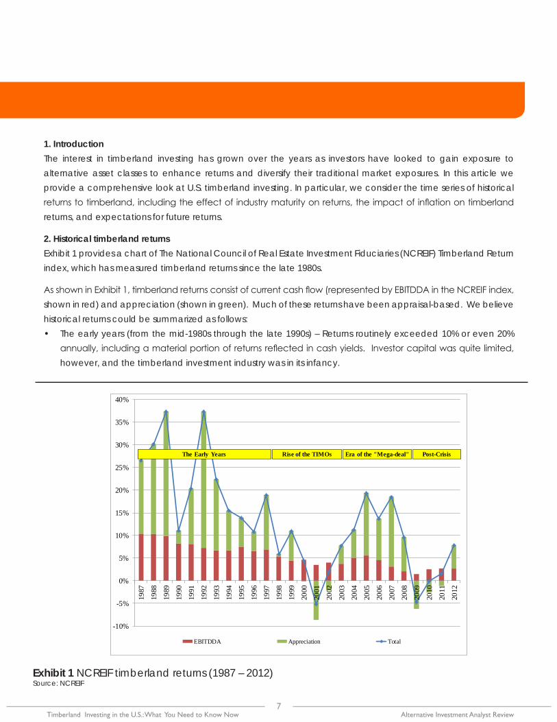
2. Historical timberland returnsExhibit 1 provides a chart of The National Council of Real Estate Investment Fiduciaries (NCREIF) Timberland Return index, which has measured timberland returns since the late 1980s.

As shown in Exhibit 1, timberland returns consist of current cash flow (represented by EBITDDA in the NCREIF index, shown in red) and appreciation (shown in green). Much of these returns have been appraisal-based. We believe historical returns could be summarized as follows: • The early years (from the mid-1980s through the late 1990s) – Returns routinely exceeded 10% or even 20%

annually, including a material portion of returns reflected in cash yields. Investor capital was quite limited, however, and the timberland investment industry was in its infancy.

Exhibit 1 NCREIF timberland returns (1987 – 2012)Source: NCREIF

-10%

-5%

0%

5%

10%

15%

20%

25%

30%

35%

40%

1987

1988

1989

1990

1991

1992

1993

1994

1995

1996

1997

1998

1999

2000

2001

2002

2003

2004

2005

2006

2007

2008

2009

2010

2011

2012

EBITDDA Appreciation Total

The Early Years Rise of the TIMOs Era of the "Mega-deal" Post-Crisis


Practitioner PerspectivesWhat a CAIA Member Should Know

• Late 1990s through early 2000s (the “Rise of the TIMOs”) – Returns suffered as timber prices retreated in the recession of 2001, though capital flows into the asset class began to increase and larger scale institutional timberland investment management companies (TIMOs) were formed.

• Early 2000s through 2008 (the era of the “Mega-Deal”) – Returns increased substantially, but in large part due to appraisals on ever-higher prices for properties. Transactions grew increasingly large (multi-billion-dollar), as integrated forest products companies took advantage of new investor capital to deconsolidate their raw material supply chains.

• 2008 to present (“After the Crash”) – Over the last several years, returns have been disappointing, dropping off significantly after the global financial crisis of 2008. While cash flows have remained positive, asset values have eroded, which roughly tracks with the decline in timber prices in connection with the crash of the housing market in the U.S. As timber prices have begun to increase, asset values have begun to recover as well.

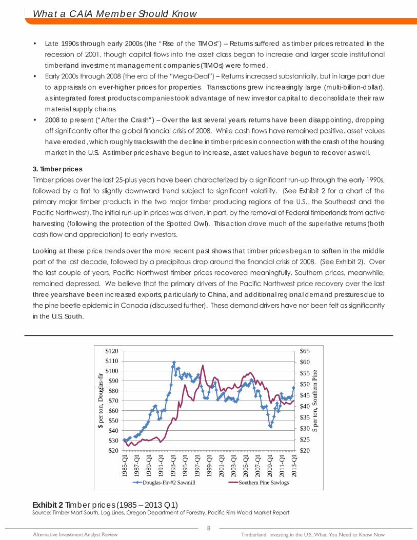
3. Timber pricesTimber prices over the last 25-plus years have been characterized by a significant run-up through the early 1990s, followed by a flat to slightly downward trend subject to significant volatility. (See Exhibit 2 for a chart of the primary major timber products in the two major timber producing regions of the U.S., the Southeast and the Pacific Northwest). The initial run-up in prices was driven, in part, by the removal of Federal timberlands from active harvesting (following the protection of the Spotted Owl). This action drove much of the superlative returns (both cash flow and appreciation) to early investors.

Looking at these price trends over the more recent past shows that timber prices began to soften in the middle part of the last decade, followed by a precipitous drop around the financial crisis of 2008. (See Exhibit 2). Over the last couple of years, Pacific Northwest timber prices recovered meaningfully. Southern prices, meanwhile, remained depressed. We believe that the primary drivers of the Pacific Northwest price recovery over the last three years have been increased exports, particularly to China, and additional regional demand pressures due to the pine beetle epidemic in Canada (discussed further). These demand drivers have not been felt as significantly in the U.S. South.

Exhibit 2 Timber prices (1985 – 2013 Q1) Source: Timber Mart-South, Log Lines, Oregon Department of Forestry, Pacific Rim Wood Market Report

$20

$25

$30

$35

$40

$45

$50

$55

$60

$65

$20$30$40$50$60$70$80$90

$100$110$120

1985

-Q1

1987

-Q1

1989

-Q1

1991

-Q1

1993

-Q1

1995

-Q1

1997

-Q1

1999

-Q1

2001

-Q1

2003

-Q1

2005

-Q1

2007

-Q1

2009

-Q1

2011

-Q1

2013

-Q1

$ pe

r ton

, Sou

ther

n Pi

ne

$ pe

r ton

, Dou

glas

-fir

Douglas-Fir-#2 Sawmill Southern Pine Sawlogs



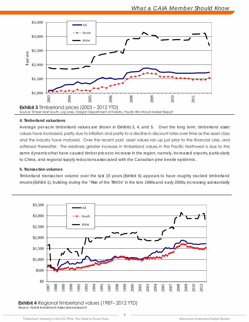
4. Timberland valuationsAverage per-acre timberland values are shown in Exhibits 3, 4, and 5. Over the long term, timberland asset values have increased, partly due to inflation and partly to a decline in discount rates over time as the asset class and the industry have matured. Over the recent past, asset values ran up just prior to the financial crisis, and softened thereafter. The relatively greater increase in timberland values in the Pacific Northwest is due to the same dynamics that have caused timber prices to increase in the region, namely, increased exports, particularly to China, and regional supply reductions associated with the Canadian pine beetle epidemic.

5. Transaction volumesTimberland transaction volume over the last 15 years (Exhibit 6) appears to have roughly tracked timberland returns (Exhibit 1), building during the “Rise of the TIMOs” in the late 1990s and early 2000s, increasing substantially

Exhibit 3 Timberland prices (2003 – 2012 YTD) Source: Timber Mart-South, Log Lines, Oregon Department of Forestry, Pacific Rim Wood Market Report

Exhibit 4 Regional timberland values (1987– 2012 YTD)Source: Forest Investment Associates research

$0

$500

$1,000

$1,500

$2,000

$2,500

$3,000

$3,500

1987

1988

1989

1990

1992

1993

1994

1995

1997

1998

1999

2000

2002

2003

2004

2005

2007

2008

2009

2010

2012

$ pe

r acr

e

All

South

PNW

$1,000

$1,500

$2,000

$2,500

$3,000

$3,500

2003

2004

2005

2006

2008

2009

2010

2011

$ pe

r acr

eAll

South

PNW



through the mid-2000s in the era of the mega-deal, and dropping off after the financial crisis. It is important to note that the era of the mega-deal was made possible by a paradigm shift in which timberlands – historically held by a relatively large number of vertically integrated forest products companies – were sold to a number of newly formed TIMOs, which were able to fund the acquisition of these assets with equity capital from institutional investors who flooded into the market at that time.

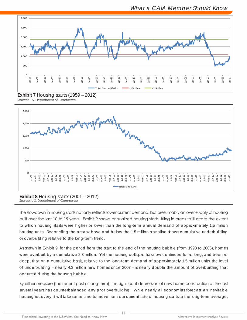
6. Increasing demand Timber demand and timber prices are driven, in large part, by housing construction. Construction demand for softwood sawtimber represents approximately 65% of total demand for the product. Of this, about two-thirds relates to new housing construction, with the remainder reflecting demand associated with repair and remodeling. Exhibit 7 depicts U.S. housing starts over the past 50 years.

Housing starts have never been this low. Historically, even in periods when housing starts declined dramatically, they recovered in less than a year. In contrast, they have now been at record low levels for nearly four years. Exhibit 8 shows housing starts over the more recent past.

Exhibit 5 Regional timberland values (2005– 2012 YTD)Source: Forest Investment Associates research

Exhibit 6 Timberland transaction volumes (1995 – 2012)Source: Forest Investment Associates research

$0

$500

$1,000

$1,500

$2,000

$2,500

$3,000

$3,500

2005

2006

2007

2008

2010

2011

2012

$ per

acre

All

South

PNW

0

1,000

2,000

3,000

4,000

5,000

6,000

7,000

8,000

9,000

1995

1996

1997

1998

1999

2000

2001

2002

2003

2004

2005

2006

2007

2008

2009

2010

2011

2012

000s

of ac

res s

old



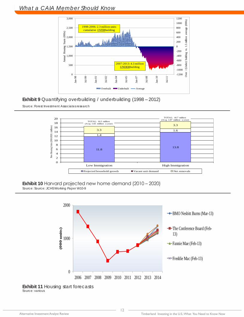
The slowdown in housing starts not only reflects lower current demand, but presumably an over-supply of housing built over the last 10 to 15 years. Exhibit 9 shows annualized housing starts, filling in areas to illustrate the extent to which housing starts were higher or lower than the long-term annual demand of approximately 1.5 million housing units. Reconciling the areas above and below the 1.5 million starts line shows cumulative underbuilding or overbuilding relative to the long-term trend.

As shown in Exhibit 9, for the period from the start to the end of the housing bubble (from 1998 to 2006), homes were overbuilt by a cumulative 2.3 million. Yet the housing collapse has now continued for so long, and been so deep, that on a cumulative basis, relative to the long-term demand of approximately 1.5 million units, the level of underbuilding – nearly 4.3 million new homes since 2007 – is nearly double the amount of overbuilding that occurred during the housing bubble.

By either measure (the recent past or long-term), the significant depression of new home construction of the last several years has counterbalanced any prior overbuilding. While nearly all economists forecast an inevitable housing recovery, it will take some time to move from our current rate of housing starts to the long-term average,

Exhibit 7 Housing starts (1959 – 2012) Source: U.S. Department of Commerce

Exhibit 8 Housing starts (2001 – 2012) Source: U.S. Department of Commerce

0

500

1,000

1,500

2,000

2,500

Jan-

01

Apr-0

1

Jul-0

1

Oct

-01

Jan-

02

Apr-0

2

Jul-0

2

Oct

-02

Jan-

03

Apr-0

3

Jul-0

3

Oct

-03

Jan-

04

Apr-0

4

Jul-0

4

Oct

-04

Jan-

05

Apr-0

5

Jul-0

5

Oct

-05

Jan-

06

Apr-0

6

Jul-0

6

Oct

-06

Jan-

07

Apr-0

7

Jul-0

7

Oct

-07

Jan-

08

Apr-0

8

Jul-0

8

Oct

-08

Jan-

09

Apr-0

9

Jul-0

9

Oct

-09

Jan-

10

Apr-1

0

Jul-1

0

Oct

-10

Jan-

11

Apr-1

1

Jul-1

1

Oct

-11

Jan-

12

Apr-1

2

Jul-1

2

Oct

-12

Jan-

13

Total Starts (SAAR)

0

500

1,000

1,500

2,000

2,500

3,000

Jan-

59

Jan-

61

Jan-

63

Jan-

65

Jan-

67

Jan-

69

Jan-

71

Jan-

73

Jan-

75

Jan-

77

Jan-

79

Jan-

81

Jan-

83

Jan-

85

Jan-

87

Jan-

89

Jan-

91

Jan-

93

Jan-

95

Jan-

97

Jan-

99

Jan-

01

Jan-

03

Jan-

05

Jan-

07

Jan-

09

Jan-

11

Jan-

13

Total Starts (SAAR) -1 St Dev +1 St Dev



Exhibit 9 Quantifying overbuilding / underbuilding (1998 – 2012)Source: Forest Investment Associates research

Exhibit 10 Harvard projected new home demand (2010 – 2020)Source: Source: JCHS Working Paper W10-9

Exhibit 11 Housing start forecasts Source: various

-1200

-1000

-800

-600

-400

-200

0

200

400

600

800

1000

1200

0

500

1,000

1,500

2,000

2,500

3,000

Jan-

98

Jul-9

9

Jan-

01

Jul-0

2

Jan-

04

Jul-0

5

Jan-

07

Jul-0

8

Jan-

10

Jul-1

1 Ove

r / (

Unde

r) bu

ildin

g vs

. 1.5

milli

on a

vera

ge (

000s

)

Annu

al Ho

using

Star

ts (0

00s)

Overbuilt Underbuilt Average

1998-2006: 2.3 million units cumulative OVERbuilding

2007:2013: 4.3 million UNDERbuilding

11.813.8

1.4

1.63.3

3.3

02468

101214161820

Low Immigration High Immigration

New

Hous

ing Un

its (2

010-2

020)

(milli

ons)

Projected household growth Vacant unit demand Net removals

TOTAL: 16.5 million (Avg. 1.65 million a year)

TOTAL: 18.7 million (Avg. 1.87 million a year)

0

1000

2000

2006 2007 2008 2009 2010 2011 2012 2013 2014

(00

0 u

nit

s)

BMO Nesbitt Burns (Mar-13)

The Conference Board (Feb-13)

Fannie Mae (Feb-13)

Freddie Mac (Feb-13)



which will only serve to further increase the amount of net underbuilding. Simultaneous with the collapse in housing starts, the share of Americans living in multi-generational family households is the highest it has been since the 1950s, having increased significantly in the past five years. In 2010, 21.6% of adults between 25 and 34 lived in this type of household, compared to 15.8% in 2000 and 11.0% in 1980. This negative household formation results in a near-term reduction of housing demand, but is not representative of the expected long-term trend.

As stated in a recent report by the Joint Center for Housing Studies of Harvard University:

…over the longer run, the most important drivers of household growth are the size and age structure of the adult population. Assuming the economic recovery is sustained in the next few years, the growth and aging of the current population alone – including the entrance of the echo boomers into adulthood – should support the addition of about 1.0 million new households per year over the next decade. The biggest unknown is the contribution of immigration to overall population growth. But even assuming net inflows are roughly half the level in the Census Bureau’s 2008 projection, the Joint Center for Housing Studies projects household growth should still average 1.18 million a year…

Using this 1.18 million figure as a base, and accounting for both net removals as well as vacant unit demand, housing starts are expected to average a minimum of 1.65 million units, as Exhibit 10 illustrates. Low immigration is half of the Census Bureau baseline immigration assumption. High immigration is the Census Bureau baseline immigration assumption.

Over the near term, what might a housing recovery look like? Exhibit 11 shows a composite of housing starts projections through 2015.

For the timberland investor, it is important to understand that asset values – and returns – are predicated on projected cash flows from harvests over a period of several decades or more. The fundamental long- term housing demand as illustrated in Exhibit 10 is therefore more relevant than the specific timing of a housing recovery, as shown in Exhibit 11.

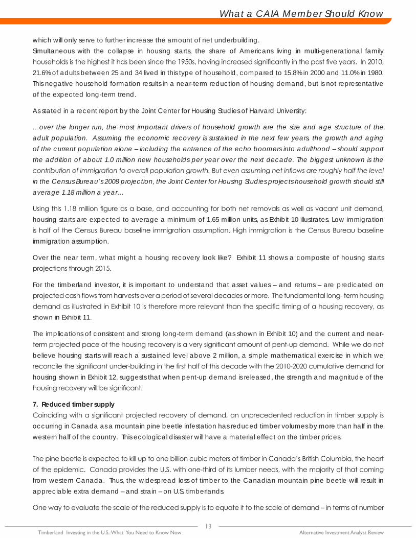
The implications of consistent and strong long-term demand (as shown in Exhibit 10) and the current and near-term projected pace of the housing recovery is a very significant amount of pent-up demand. While we do not believe housing starts will reach a sustained level above 2 million, a simple mathematical exercise in which we reconcile the significant under-building in the first half of this decade with the 2010-2020 cumulative demand for housing shown in Exhibit 12, suggests that when pent-up demand is released, the strength and magnitude of the housing recovery will be significant.

7. Reduced timber supplyCoinciding with a significant projected recovery of demand, an unprecedented reduction in timber supply is occurring in Canada as a mountain pine beetle infestation has reduced timber volumes by more than half in the western half of the country. This ecological disaster will have a material effect on the timber prices.

The pine beetle is expected to kill up to one billion cubic meters of timber in Canada’s British Columbia, the heart of the epidemic. Canada provides the U.S. with one-third of its lumber needs, with the majority of that coming from western Canada. Thus, the widespread loss of timber to the Canadian mountain pine beetle will result in appreciable extra demand – and strain – on U.S. timberlands.

One way to evaluate the scale of the reduced supply is to equate it to the scale of demand – in terms of number



of housing starts. Exhibit 14 illustrates that the reduction in annual supply from Canada would equate to the same amount of wood that would be consumed in approximately 400,000 housing starts. Further, exports to China – which effectively reduce supply that would otherwise be available for U.S. based demand – equate to approximately the demand from 200,000 housing starts.

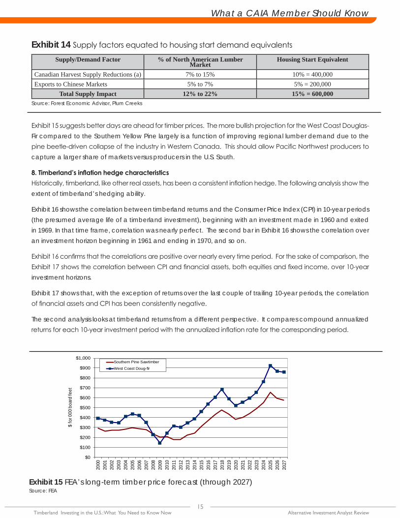
What, then, is the net impact of the supply and demand factors discussed above? Future timber prices are expected to rise substantially from their current historic lows. Exhibit 15 reflects forecasts for Southern Yellow Pine and West Coast Douglas-Fir over the next 15 years from Forest Economic Advisors (FEA), the dominant global forest products economist and research firm providing long-term price projections to the industry.

Exhibit 12 Theoretical housing starts in the second half of this decadeSource: Forest Investment Associates research

Extent of Pine

Beetle Infestation

Extent of Pine

Beetle Infestation

Exhibit 13 The Canadian Pine Beetle epidemicSource: Natural Resources Canada

0

500

1,000

1,500

2,000

2,500

3,000

2010 A 2011 A 2012 A 2013 E 2014 E 2015 E 2016 E 2017 E 2018 E 2019 E 2020 E

000s

of H

ousin

g St

arts

High immigration case

Low immigration case

2010-2012Actual housing starts to date

2013-2015Near term composite

projections

2016-2020Implied magnitude of

pent up housing demand



Source: FEA

Exhibit 14 Supply factors equated to housing start demand equivalents

Supply/Demand Factor % of North American Lumber Market

Housing Start Equivalent

Canadian Harvest Supply Reductions (a) 7% to 15% 10% = 400,000Exports to Chinese Markets 5% to 7% 5% = 200,000

Total Supply Impact 12% to 22% 15% = 600,000

Exhibit 15 suggests better days are ahead for timber prices. The more bullish projection for the West Coast Douglas-Fir compared to the Southern Yellow Pine largely is a function of improving regional lumber demand due to the pine beetle-driven collapse of the industry in Western Canada. This should allow Pacific Northwest producers to capture a larger share of markets versus producers in the U.S. South.

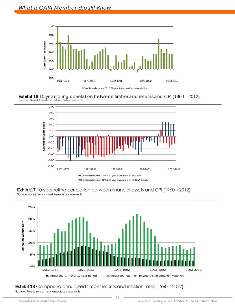
8. Timberland’s inflation hedge characteristicsHistorically, timberland, like other real assets, has been a consistent inflation hedge. The following analysis show the extent of timberland’s hedging ability.

Exhibit 16 shows the correlation between timberland returns and the Consumer Price Index (CPI) in 10-year periods (the presumed average life of a timberland investment), beginning with an investment made in 1960 and exited in 1969. In that time frame, correlation was nearly perfect. The second bar in Exhibit 16 shows the correlation over an investment horizon beginning in 1961 and ending in 1970, and so on.

Exhibit 16 confirms that the correlations are positive over nearly every time period. For the sake of comparison, the Exhibit 17 shows the correlation between CPI and financial assets, both equities and fixed income, over 10-year investment horizons.

Exhibit 17 shows that, with the exception of returns over the last couple of trailing 10-year periods, the correlation of financial assets and CPI has been consistently negative.

The second analysis looks at timberland returns from a different perspective. It compares compound annualized returns for each 10-year investment period with the annualized inflation rate for the corresponding period.

Source: Forest Economic Advisor, Plum Creeks

Exhibit 15 FEA’s long-term timber price forecast (through 2027)

$0

$100

$200

$300

$400

$500

$600

$700

$800

$900

$1,000

2000

2001

2002

2003

2004

2005

2006

2007

2008

2009

2010

2011

2012

2013

2014

2015

2016

2017

2018

2019

2020

2021

2022

2023

2024

2025

2026

2027

$ fo

r 000

boa

rd fe

et

Southern Pine Sawtimber

West Coast Doug-fir



Exhibit 16 10-year rolling correlation between timberland returns and CPI (1960 – 2012) Source: Forest Investment Associates research

Exhibit 18 Compound annualized timber returns and inflation rates (1960 – 2012) Source: Forest Investment Associates research

Exhibit17 10-year rolling correlation between financial assets and CPI (1960 – 2012) Source: Forest Investment Associates research

-0.20

0.00

0.20

0.40

0.60

0.80

1.00

1962-1971 1972-1981 1982-1991 1993-2002 2003-2012

Corr

elat

ion

Coef

ficie

nts

Correlation between CPI & 10 year timberland investment returns

-1.00

-0.80

-0.60

-0.40

-0.20

0.00

0.20

0.40

0.60

0.80

1.00

1962-1971 1972-1981 1982-1991 1992-2001 2002-2012

Corr

elat

ion

Coef

ficie

nts

Correlation between CPI & 10 year investment in S&P 500

Correlation between CPI & 10 year investment in LT Gov't Bonds

0%

5%

10%

15%

20%

25%

1963-1972 1973-1982 1983-1992 1993-2002 2003-2012

Com

poun

d An

nual

Rate

Annualized CPI over 10 year period Annualized return on 10 year US timberland investment



is a green bar (representing the annualized timberland return) lower than a black and white bar (representing the annualized inflation rate).

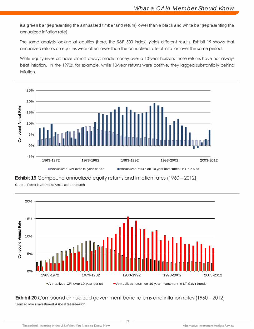
The same analysis looking at equities (here, the S&P 500 index) yields different results. Exhibit 19 shows that annualized returns on equities were often lower than the annualized rate of inflation over the same period.

While equity investors have almost always made money over a 10-year horizon, those returns have not always beat inflation. In the 1970s, for example, while 10-year returns were positive, they lagged substantially behind inflation.

Exhibit 19 Compound annualized equity returns and inflation rates (1960 – 2012) Source: Forest Investment Associates research

Exhibit 20 Compound annualized government bond returns and inflation rates (1960 – 2012)Source: Forest Investment Associates research

-5%

0%

5%

10%

15%

20%

25%

1963-1972 1973-1982 1983-1992 1993-2002 2003-2012

Com

poun

d An

nual

Rat

e

Annualized CPI over 10 year period Annualized return on 10 year investment in S&P 500

0%

5%

10%

15%

20%

1963-1972 1973-1982 1983-1992 1993-2002 2003-2012

Com

poun

d An

nual

Rat

e

Annaulized CPI over 10 year period Annaulized return on 10 year investment in LT Gov't bonds

Analysis of long-term government bonds vs. inflation yield a similar result, as seen in Exhibit 20. As this exhibit shows, bond investors before the 1980s lost money to inflation.

9. SummaryWhile timberland returns have been weak the last few years as housing starts have fallen to historic lows, supply and demand factors remain extremely favorable for the asset class. Housing starts, having been at depressed levels for such a long time, are poised for a very sharp recovery, and may even reach unprecedented levels (above two million starts annually) for several years in the second half of this decade. At the same time, on the supply side, the Canadian mountain pine beetle has reduced available supply coming from north of the border, which historically has accounted for approximately one-third of the U.S. lumber market. Add to that dynamic the steadily increasing demand from China, and all signs point to a significant improvement in timber prices over the next several years. This is expected to not only drive premium returns for investors, but continue to provide them. Our research underscores Forest Economic Advisor’s (FEA)’s bullish timber price forecast over the long term. Further, timber looks to be a very effective hedge against inflation.

Author BiosThomas J. Healey is a retired Goldman, Sachs partner, a former Assistant Secretary of the U.S. Treasury for Domestic Finance under President Reagan and an adjunct professor at Harvard University’s John F. Kennedy School of Government where he teaches the course in Financial Institutions and Markets. Tom received a B.A. from Georgetown University and an M.B.A. from Harvard Business School.

Tim Corriero is a Managing Director at FIA Timber Partners, a timberland asset management company. Prior to his current role, Tim was an investment banker with Goldman Sachs focusing on the forest products industry. He also previously worked as a corporate attorney for Shearman & Sterling. Tim holds a B.A. from Colgate University and a J.D. from Harvard Law School.

Scott Bond is Vice President and Director of Marketing & Client Relations at Forest Investment Associates, a timberland asset management company. Scott has been in financial services since 1984, which has included leading the commercial business development efforts for a major bank as well as positions in corporate and mortgage banking. Scott holds a B.S. in Business Administration from Trinity University and an M.B.A. from the University of North Carolina.



timberland investing in the us: what you need - caia association

Documents