time-dependent deformation behavior of prestressed high...
TRANSCRIPT

RESEARCH REPORT 580-6
TIME-DEPENDENT DEFORMATION BEHAVIOR OF
PRESTRESSED HIGH PERFORMANCE CONCRETE
BRIDGE BEAMS
K. A. Byle, Ned H. Burns, and Ramón L. Carrasquillo
CENTER FOR TRANSPORTATION RESEARCHBUREAU OF ENGINEERING RESEARCHTHE UNIVERSITY OF TEXAS AT AUSTIN
���������

Technical Report Documentation Page
�����������
�� �������������
������������������������� ����������!��"##$�%���
���������&#�
'��(������)
*����$��#�+�,-(�$�
�./0�&010&0��&0�'�/��.'�20��3.'��'��1�0,��0,,0&
�.���10��'�/�"0�"'"�0�0�2�.&�0�20�/,���1��4�����%�'�%#��5#����"�+�
)���-6��7�8
9�����2:$�;��+����2-���;�#�+����<��"#��#�=-�$$�
���1��4�����%�'�%#��5#������������
�������
���� ��>�?������7���.,8���1��4�����%�'�%#��5#����#���#�+��++����
"�����4�����#�����#��������#��6
�6��?�������:��4���@#��#��-���
������+������;�,-������
�-���;����)�)�������
����"���#�������#����
�����
� ���:����4�������#�+�1����+�"�����+
�����#��6��������������������
7�����A����)8
����,��������%��%���:�#���#�+��++����
��@#��&��#������4���#�����#���
����#��6�#�+����6��$�%:���#��4���,������"����-�����&�������
1�'��2�@�����
�-���;����)�)� ����� �*��,��������%��%���:�"�+�
����,-��$����#�:����
1��B������+-��+����������#����C�6�6����+��#$���%6C#:��+������#����
�����(��#�
�C�$���4-$$���#$�����������+�6�%6����4���#��������������@#���:���?�*�(��+%��(�#���C�6���#��$��%6���#�%��%
4���� ����� �� *����� ������ C���� ����-����+� #�+� �������+� ��� 6�� 4��$+�� �6�� ����-����+� ?�(�#��� C���
4#(���#�+� -���%� ����� ���+�#����� $�C���$#@#���� ����������%� ��#�+�� #�+� �������� C�6� +���%�� �����������
����%6�� (�C��������� #�+� ��� �/1#�������+����+��� �#�(��;� +�4$�����;� ��#��� #� 6�� ������ �4� %�#��:� �4� 6�
����������%���#�+�;�#�+���#���+����(-�����#���+��#��C������#�-��+�4�����#��4����4�6������������%�4�����-��$
�� ���6�� #4��� ����$����� �4� 6�� ��������� +��>�� .����#$� (�#�� �����#-���� #� ��+��#�� C���� #$��� ��#�-��+
+-���%�6#����������+;�#$$�C��%�4���6����#�-�������4������#-���%�#+����������6��(�#��+��6�
�6�� ��#�-��+� ����+����+��� �#�(��;� +�4$�����;� #�+� ��������� $������ #� ��+��#�� C���� ����#��+� C�6� ���-$�
�(#���+�-���%���,��'�#�+�1".����+��������6��=-����1��+�������C����#$����#+��-���%�#��#�#$:��#$��������
��6�+� 6#�C#�� +���$���+� ��� #� ����-��� ����#+�6��� ���%�#��� �6�� #�#$:��#$� ����������6�+� ���+���+� 6�
����+����+���(�6#������4�6������-����+�(�#���4#��$:�#��-�#�$:;�C6�$��6����,��'�#�+�1".���6�+��:��$+�+
��#��-�#�����+�������
�� ��� �4� �#�(��� #�+� +�4$������ �-$��$����� C���� +���$���+� (#��+� ��� 6�� #�#$:��#$� �������� ��6�+� #�+� 6�
��#�-��+����������$������#�+��#���#$�����������4���6������-����+�(�#�����6���=-#�����4��� 6�����-$��$����
C����C�$$� �-��+� 4��� ���%�#����%� ��� #� ����-��;� #$6�-%6� 6�:� ��-$+� #$��� (�� -��+� 4��� 6#�+� �#$�-$#������ �6�
��������:��4��#�(������+��������6����+-$-���4��$#����:�#���$�#���#�+�6������������%�4����+��#��4����+���6�
(�#���C#��������%#�+�-���%�6���������+��-$��$�����
�)��9�:� ��+�
��%6����4���#������������(��+%��;�����+����+��
+�4���#����(�6#����;���@#���:���?�*�%��+���
����&����(-����,#����
���������������6���+��-�������#�#�$#($����6���-($��
6��-%6�6��#���#$����6���#$�.�4���#����,������;
,����%4��$+;�3��%���#�������
����,��-��:�"$#���4��7�4������8
?��$#���4��+
����,��-��:�"$#���4��7�4�6����#%�8
?��$#���4��+
��������4��#%��
� �
����1����
Form DOT F 1700.7 (8-72) Reproduction of completed page authorized

TIME-DEPENDENT DEFORMATION BEHAVIOR OF PRESTRESSEDHIGH PERFORMANCE CONCRETE BRIDGE BEAMS
by
Kenneth Arlan Byle,
Ned H. Burns,
and
Ramón L. Carrasquillo
Research Report 580-6
Research Project 9-580“High Performance Concrete for Bridges”
Conducted for the
TEXAS DEPARTMENT OF TRANSPORTATION
in cooperation with the
U.S. DEPARTMENT OF TRANSPORTATIONFEDERAL HIGHWAY ADMINISTRATION
by the
CENTER FOR TRANSPORTATION RESEARCHBUREAU OF ENGINEERING RESEARCH
THE UNIVERSITY OF TEXAS AT AUSTIN
September 1998

ii

iii
DISCLAIMERS
The contents of this report reflect the views of the authors, who are responsible for thefacts and the accuracy of the data presented herein. The contents do not necessarily reflectthe official views or policies of the Federal Highway Administration (FHWA) or the TexasDepartment of Transportation (TxDOT). This report does not constitute a standard,specification, or regulation.
There was no invention or discovery conceived or first actually reduced to practice inthe course of or under this contract, including any art, method, process, machine,manufacture, design or composition of matter, or any new and useful improvement thereof,or any variety of plant, which is or may be patentable under the patent laws of the UnitedStates of America or any foreign country.
NOT INTENDED FOR CONSTRUCTION, BIDDING, OR PERMIT PURPOSES
R. L. Carrasquillo, P.E. (Texas No. 63881)Research Supervisor
ACKNOWLEDGMENTS
The researchers acknowledge the invaluable assistance provided by Mary Lou Ralls(DES), TxDOT project director for this study. Also appreciated is the guidance provided bythe other members of the project monitoring committee, which includes J. P. Cicerello(DES), A. Cohen (DES), W. R. Cox (CMD), N. Friedman (DES), D. Harley (FHWA), G.Lankes (MAT), L. Lawrence (MAT), L. M. Wolf (DES), and T. M. Yarbrough (CSTR).
Prepared in cooperation with the Texas Department of Transportation and the U.S.Department of Transportation, Federal Highway Administration.

iv

v
TABLE OF CONTENTS
CHAPTER 1. INTRODUCTION ......................................................................................... 11.1 Background ............................................................................................................... 1
1.1.1 Historical Overview ......................................................................................... 11.1.2 Developments in the Prestressed Concrete Industry ........................................ 11.1.3 Development of High Performance Concrete .................................................. 21.1.4 High Performance Concrete in Bridges............................................................ 2
1.2 Deformation Behavior of Prestressed Concrete Beams ............................................ 31.2.1 Causes of Camber and Deflection .................................................................... 31.2.2 Parameters Affecting Camber and Deflection.................................................. 61.2.3 Prestress Losses................................................................................................ 7
1.3 Research Program ..................................................................................................... 81.4 Objectives of This Study........................................................................................... 91.5 Organization of Report.............................................................................................. 9
CHAPTER 2. REVIEW OF LITERATURE ........................................................................ 112.1 Introduction ............................................................................................................... 112.2 High Strength Concrete............................................................................................. 11
2.2.1 Production and Implementation of High Strength Concrete............................ 112.2.2 Material Properties of High Strength Concrete................................................ 12
2.3 Field Instrumentation Programs................................................................................ 142.4 Previous Studies of Time-Dependent Behavior ........................................................ 142.5 Methods of Estimating Time-Dependent Behavior .................................................. 15
2.5.1 Code Provisions ............................................................................................... 152.5.2 Analytical Methods .......................................................................................... 16
CHAPTER 3. BRIDGE DETAILS, INSTRUMENTATION,AND COMPANION TESTS ........................................................................ 19
3.1 Introduction ............................................................................................................... 193.2 Bridge Details............................................................................................................ 19
3.2.1 General ............................................................................................................. 193.2.2 Bridge Girder Details ....................................................................................... 223.2.3 Composite Bridge Details and Support Conditions ......................................... 243.2.4 Instrumented Beams......................................................................................... 26
3.3 Instrumentation.......................................................................................................... 293.3.1 Selection of Instrumentation ............................................................................ 293.3.2 Concrete Surface Strain Measurement ............................................................. 313.3.3 Internal Strain Measurement ............................................................................ 333.3.4 Internal Temperature Measurement ................................................................. 353.3.5 Long-Term Camber and Deflection Measuring System .................................. 39
3.4 Data Acquisition........................................................................................................ 41

vi
3.4.1 General ............................................................................................................. 413.4.2 Data Acquisition System.................................................................................. 413.4.3 Data Reduction................................................................................................. 42
3.5 Materials.................................................................................................................... 433.5.1 Precast U-Beams .............................................................................................. 433.5.2 Precast Deck Panels ......................................................................................... 433.5.3 Cast-in-Place Deck Slabs ................................................................................. 44
3.6 Companion Tests....................................................................................................... 443.6.1 General ............................................................................................................. 443.6.2 Modulus of Elasticity ....................................................................................... 453.6.3 Compressive Strength ...................................................................................... 453.6.4 Creep and Shrinkage ........................................................................................ 463.6.5 Coefficient of Thermal Expansion ................................................................... 47
CHAPTER 4. FIELD WORK ............................................................................................... 494.1 Introduction ............................................................................................................... 49
4.1.1 Coordination with Contractors ......................................................................... 494.1.2 Chapter Format................................................................................................. 49
4.2 Preparation of Instrumentation.................................................................................. 494.3 Precast Operations..................................................................................................... 51
4.3.1 Precast Beams .................................................................................................. 514.3.2 Precast Deck Panels ......................................................................................... 57
4.4 Cast-in-Place Decks .................................................................................................. 594.4.1 Preparation ....................................................................................................... 594.4.2 Instrumentation................................................................................................. 604.4.3 Casting.............................................................................................................. 61
4.5 Problems Encountered in the Field ........................................................................... 624.5.1 Difficulties with Instrumentation Placement.................................................... 624.5.2 Damaged Instrumentation ................................................................................ 634.5.3 Measurements................................................................................................... 64
CHAPTER 5. OBSERVED BEHAVIOR............................................................................. 675.1 Introduction ............................................................................................................... 675.2 Companion Test Results ........................................................................................... 67
5.2.1 Concrete Compressive Strength ....................................................................... 675.2.2 Elastic Modulus of Concrete ............................................................................ 705.2.3 Creep and Shrinkage Properties of Concrete ................................................... 72
5.3 Field Measurements .................................................................................................. 765.3.1 Camber and Deflection..................................................................................... 765.3.2 Surface Strain at the Center of Gravity of the Prestressing Strands................. 865.3.3 Internally Measured Strain at the Center of Gravity
of the Prestressing Strands ............................................................................... 885.3.4 Measured Strain Profiles at Midspan ............................................................... 95

vii
5.3.5 Temperature Gradients ..................................................................................... 1015.3.6 Thermally Induced Camber and Deflection ..................................................... 107
5.4 Comparison of Measured Behavior........................................................................... 1105.4.1 Camber and Deflection..................................................................................... 1105.4.2 Prestressing Strand Strain................................................................................. 1245.4.3 Midspan Strain Profiles at Release................................................................... 134
CHAPTER 6. ANALYTICAL METHODS FOR PREDICTINGTIME-DEPENDENT BEHAVIOR............................................................... 139
6.1 Introduction ............................................................................................................... 1396.2 AASHTO................................................................................................................... 1396.3 PCI Design Handbook: Prestress Losses, Camber, and Deflection .......................... 151
6.3.1 Prestress Losses................................................................................................ 1516.3.2 Camber and Deflection..................................................................................... 159
6.4 Analytical Time-Step Method................................................................................... 1726.4.1 General ............................................................................................................. 1726.4.2 Prestress Losses................................................................................................ 1726.4.3 Camber and Deflection..................................................................................... 182
6.5 Proposed Multipliers for Estimating Time-Dependent Camber and Deflection....... 1956.5.1 Development of Proposed Multipliers ............................................................. 1956.5.2 Prediction of Camber and Deflection using Proposed Multipliers .................. 199
CHAPTER 7. SUMMARY, CONCLUSIONS, AND RECOMMENDATIONS................. 2117.1 Summary ................................................................................................................... 2117.2 Conclusions ............................................................................................................... 2117.3 Recommendations ..................................................................................................... 214
REFERENCES...................................................................................................................... 215APPENDIX A: DEBONDING DETAILS............................................................................ 221

viii
1
CHAPTER 1. INTRODUCTION
1.1 BACKGROUND
1.1.1 Historical Overview
Most of the bridges that are currently part of the United States infrastructure wereconstructed following the passage of the Federal Aid Highway Act in 1956 (1). Today, manyof these bridges do not meet current federal and state design standards for geometry, strength,or average daily vehicular traffic. This can be attributed to the excessive demand placed onthe infrastructure over the 20- to 30-year period following construction. During that timeperiod, the use of the infrastructure system rapidly increased as tourism, the interstate trade ofgoods by truck, and the mobilization of people across the nation grew to be economic forces.Yesterday’s bridges were not designed for the size, weight, and volume of today’s car andtruck traffic. Consequently, a large percentage of these bridge structures are in need ofsubstantial improvement or complete replacement.
It was also shortly after 1956 that the prestressed concrete industry began to flourish.A construction project as large as the interstate system demanded cost-effective structuralsystems. The development of standardized beam sections, most notably the I-shaped section,made prestressed concrete an efficient alternative for bridge superstructures. However, thestrength and durability properties of the concrete used in those bridges are inferior to those ofthe high strength concrete being developed and implemented today.
1.1.2 Developments in the Prestressed Concrete Industry
Recent developments in the prestressing industry can be utilized to provideeconomical design solutions to satisfy the increasing demand for bridge replacement. Onesuch development is the use of 15.2 mm-diameter low-relaxation prestressing strand in placeof the more common 12.7 mm-diameter strand. The 15.2 mm-diameter strand has 40 percentmore area than the 12.7 mm-diameter strand. When it is used in the standard 50 mm by 50mm grid spacing, the larger strand has the potential for providing 40 percent moreprestressing force.
In order to efficiently utilize the larger force that can be developed with the 15.2 mm-diameter strands, concrete with higher compressive strength needed to be developed. Thetypical compressive strength of concrete used for prestressed beams in the 1950’s wasbetween 27.6 and 34.5 MPa. Peterman and Carrasquillo (2) were able to produce highquality concrete with compressive strengths in the 62.1 MPa to 82.7 MPa range at 56 daysusing conventional batching procedures and materials that were readily available in the stateof Texas. To utilize the benefits afforded by high strength concrete, the ability to produce itin the field on a consistent basis is needed. Additionally, it is important to be able to producehigh strength concrete using materials that are readily available in the region of the project.The use of high strength concrete along with the 15.2 mm-diameter strands can result in

2
longer spans, fewer beams per span, more efficient cross-sections, and fewer substructureunits. As a direct result, construction costs can be reduced significantly.
In addition to the development of larger diameter prestressing strands and higherstrength concrete, the development of more efficient beam cross-sections has helped increasethe cost effectiveness of prestressed concrete bridge structures. The Texas U40 and U54beam sections were developed to provide more structural efficiency than that of the standardTexas Type C and AASHTO Type IV, respectively (1). The results of a parametric study byRussell (3) showed that the use of high strength concrete and 15.2 mm-diameter strands withthe Texas Type U54B section would result in wider beam spacing and longer spans than withthe AASHTO Type IV section. The Texas Type U54A and U54B sections were utilized forthe bridge in this study.
1.1.3 Development of High Performance Concrete
High performance concrete, as opposed to high strength concrete, refers to concretethat satisfies any number of significant long-term performance requirements rather thancompressive strength alone. High performance concrete (HPC) differs from normal concretein that it is engineered to meet specific strength and durability requirements, depending onthe particular application. A working definition of high performance concrete (HPC) basedon long-term performance criteria has been developed by Goodspeed et al. (4) underdirection of the Federal Highway Administration (FHWA). The objective of this definitionwas to assist in the implementation of HPC in highways and bridge structures by makingspecification of HPC more straightforward for engineers.
The proposed HPC definition was based on four strength and four durabilityparameters. The strength parameters were compressive strength, elastic modulus, shrinkage,and creep. The durability parameters were freeze-thaw, scaling resistance, abrasionresistance, and chloride penetration. For each of these parameters, performance grades fromone to four were defined based on a relationship between severity of the field condition andrecommended performance level. In addition, standard testing methods were defined tomeasure performance for each parameter (4). The development of the HPC definition allowsengineers to specify concrete strength and durability requirements based on the structuralapplication (beam, deck, or substructure) and environmental conditions of the project site.Quality assurance and quality control are vital to the implementation and success of highperformance concrete.
1.1.4 High Performance Concrete in Bridges
High performance concrete used in bridge structures can provide an increase in long-term durability coupled with several economic benefits. The use of HPC for bridge beamsand decks can result in initial benefits, such as fewer spans, beams, and substructures, as wellas long-term benefits, such as reduced maintenance, longer service life, and lower life-cyclecosts.
Widespread use of HPC in bridge structures requires the monitoring of severalbridges in the field to develop a data base of knowledge on the long-term performance of
3
bridge beams and decks. Currently there is very little information for the engineer orcontractor to turn to for guidance in predicting the behavior ofstructural members constructed with high performance concrete.
During the design and construction of a bridge, the engineer and contractor mustestimate the long-term deflection behavior of the prestressed concrete beams. Because of theuncertainty in determining properties of concrete, the prediction of camber at the beginningof service life for a composite bridge deck is very difficult. Factors such as creep, shrinkage,the elastic modulus of the concrete, and relaxation of the prestressing strands continuallychange with time. This makes an accurate estimation of long-term behavior difficult toaccomplish. The use of HPC in bridge beams and decks can only increase this difficulty. Asmore information is gathered, better estimates of long-term behavior can be made for bridgestructures constructed using HPC; at the same time, engineers and contractors may becomemore comfortable using this new technology for bridges.
1.2 DEFORMATION BEHAVIOR OF PRESTRESSED CONCRETE BEAMS
For composite prestressed concrete beam bridges with span lengths exceeding 40meters, the serviceability limit state becomes very important. In many cases it becomes thecontrolling limit state, rather than the allowable stress or ultimate strength limit states thatusually control designs. The accurate prediction of camber and deflection behavior ofprestressed concrete beams becomes essential when considering the serviceability limit state.Camber differentials between adjacent beams upon erection cause the contractor to add moreconcrete to the cast-in-place slab to level it out while maintaining minimum thicknessrequirements at the same time. The additional concrete needed to level out the deck slabproduces an increase in the deflection of the beams. If the beams have too much camber ordeflection, the driving surface will be rough and unpleasant for motorists using the bridge.Also, a downward deflection creates an aesthetically displeasing bridge for the public. Theaccurate prediction of long-term camber and deflection can reduce or eliminate theseproblems and ease the construction of the bridge.
1.2.1 Causes of Camber and Deflection
Long-term camber and deflection in prestressed concrete beams are caused by acombination of sustained loads, transient loads, and time-dependent material properties thataffect sustained loads. Precise prediction of long-term camber is extremely difficult becausethe net camber is usually the small difference between several large components of camberand deflection.
At transfer of the prestressing force, the downward deflection caused by the beamself-weight (�beam) is opposed by a larger upward deflection caused by the prestressing force(�ps), whose line of action is a distance ‘e’ below the center of gravity of the beam cross-section. These components of camber and deflection are given in Eqs. 1.1 and 1.2.
�������
�
�
��� ������������������������������������������������������������
4
�����
�
��
� �������������������������������������������������������������������
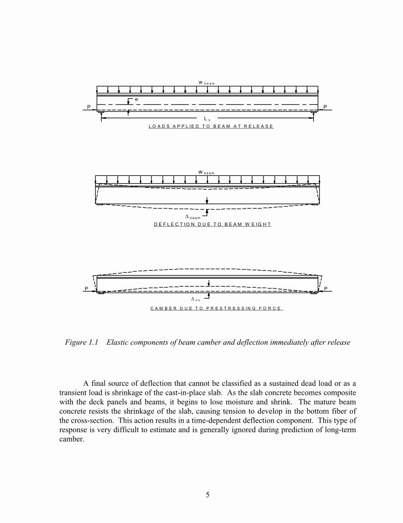
A net upward deflection (camber) is induced in the beam immediately after transferdue to elastic action only. The magnitude of the initial camber is the difference between theupward component due to prestressing and the downward component due to the beam weight(�ps - �beam). The magnitude of this camber can be rather small for long spans, even thougheach individual component is quite large.
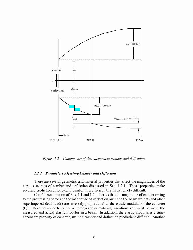
Figure 1.1 illustrates the components of initial camber at release for the beams in thisstudy. The strands in these beams were debonded at the ends. The debonded strands reducethe eccentricity and prestressing force at the ends of the beam. The effect that the debondedstrands have on �ps is minimal. Therefore, the equation for initial camber due to theprestressing force has been simplified in Figure 1.1 to exclude the effects of debonding.Each component of camber and deflection increases with time, due to the effects of creep.The beam camber will continue to increase up to the time of additional loading. Figure 1.2shows how each component increases with time.
After the beams are erected in the bridge, additional sustained loads are applied whichcause immediate elastic deflection in the beams. These sustained loads include precast deckpanels, cast-in-place slabs, guardrails, and surface overlays. The first two sources are usuallyresisted by the beam alone, while the last two sources are resisted by the composite decksection. The deflections caused by each sustained load increase with time due to the effectsof the time-dependent material properties. However, the increase is usually small because thebeam concrete is quite mature by that time and some of the additional load is resisted by astiffer composite section. The composite section will also slow down the growth of theinitial camber and deflection components that occur just after release. Figure 1.2 shows howthe beam deflection is affected by superimposed loads.
Other sources of deflection can be classified as transient in nature because the loadsare applied to the beams for only a short period of time. Temperature gradients in thecomposite bridge section can induce daily fluctuations in camber. If the top portion of thesection is heated more than the bottom portion, the top tends to expand more, which inducesadditional camber in the beam. Maximum thermally induced camber occurs on sunny daysduring the afternoon when solar radiation is the most intense. The effects of thermalgradients are removed at night when the temperature of the cross-section becomes uniform.Another temporary source of deflection is due to live loads caused by vehicular traffic on thebridge during its service life. These types of loads are not considered in determining the netlong-term camber in the bridge. However, temporary camber induced by thermal gradientscan have an impact on the roughness of the riding surface.
5
� � � � � �� � � � � � � � �� � � �� � � � �
� � � � �
��
� �
�
� � � � �� � �� � � � �� � � �� �� �
� � � ��
� �� ��
� � � � �� � � � �� � � � �� � � � � �
� � �
� �
Figure 1.1 Elastic components of beam camber and deflection immediately after release
A final source of deflection that cannot be classified as a sustained dead load or as atransient load is shrinkage of the cast-in-place slab. As the slab concrete becomes compositewith the deck panels and beams, it begins to lose moisture and shrink. The mature beamconcrete resists the shrinkage of the slab, causing tension to develop in the bottom fiber ofthe cross-section. This action results in a time-dependent deflection component. This type ofresponse is very difficult to estimate and is generally ignored during prediction of long-termcamber.
6
�
����������
������
����
!" # $% &�'!
���
�����
����(
��������������
������������
�����)���(���������
Figure 1.2 Components of time-dependent camber and deflection
1.2.2 Parameters Affecting Camber and Deflection
There are several geometric and material properties that affect the magnitudes of thevarious sources of camber and deflection discussed in Sec. 1.2.1. These properties makeaccurate prediction of long-term camber in prestressed beams extremely difficult.
Careful examination of Eqs. 1.1 and 1.2 indicates that the magnitude of camber owingto the prestressing force and the magnitude of deflection owing to the beam weight (and othersuperimposed dead loads) are inversely proportional to the elastic modulus of the concrete(Ec). Because concrete is not a homogeneous material, variations can exist between themeasured and actual elastic modulus in a beam. In addition, the elastic modulus is a time-dependent property of concrete, making camber and deflection predictions difficult. Another

7
material parameter, namely the unit weight of the concrete, directly affects the deflectioncomponents due to the beam and other superimposed distributed loads. This property can beestimated with relatively high accuracy.
Creep of concrete affects the time-dependent growth of camber and deflection due tosustained loads, as shown in Figure 1.2. Creep, shrinkage, and relaxation of the prestressingstrands interact with each other to affect the prestressing force over time. This is discussedfurther in Sec. 1.2.3.
Several geometric parameters shown in the equations in Figure 1.1 can have asignificant effect on camber and deflection. The moment of inertia of the cross-section (I) isinversely proportional to the camber and deflection components. The combination of theelastic modulus (Ec) and the moment of inertia (I) represents the stiffness of the beam in theelastic range. A more significant parameter that affects camber and deflection is the spanlength (Ls). Camber due to the prestressing force is proportional to the square of the spanlength. Deflections due to the beam, panel, and slab uniform loads are proportional to thefourth power of the span length. For long spans, the camber and deflection components canbecome extremely sensitive to small variations in the span length.
1.2.3 Prestress Losses
Prestress losses reduce the total prestressing force applied to the beam over time,resulting in a reduction of the beam camber over time. Several different sources of prestressloss occurring at different times contribute to the long-term prestress loss in a beam.
The initial loss of prestress is due to elastic shortening when transfer occurs. Sincethe strands are bonded to the beam during transfer, they will shorten with the beam as theforce is applied to the beam cross-section.
Thermal losses may occur prior to release if the temperature of the strands is lower atthe time of stressing than at the time of casting. During that time period, heating of the freestrand results in a loss of stress because the strand tends to lengthen as it increases intemperature. A portion of strand relaxation, which is a loss of stress due to a constant strainapplied to the strand, also occurs prior to transfer.
It is the time-dependent properties of the steel and the concrete that make the loss ofprestress over time a complex issue. Creep of the concrete is the increase in deformation, orcompressive strain, caused by the presence of an applied stress. Shrinkage of the concrete isa volume change in the concrete that occurs as moisture leaves the beam, resulting in acompressive strain. Additional relaxation of the strand occurs over a long period of time. Allof these factors affect the loss of prestress over time. A complex interaction exists betweencreep, shrinkage, and steel relaxation as they pertain to prestress loss. A reduction in thesteel stress due to relaxation causes less creep loss to occur, which in turn causes less steelrelaxation to occur. Furthermore, the existing environmental conditions greatly affect thetime-dependent creep and shrinkage properties of concrete. Prestress losses are also reducedwhen superimposed loads are placed on the beam or composite section. Because of theircomplexity, long-term prestress losses can only be estimated, and the amount of lossattributed to each source is impossible to determine with precision.
8
1.3 RESEARCH PROGRAM
The primary objective of this research program was to develop guidelines for thedesign and construction of highway bridge structures that utilize high performance concrete.These guidelines were developed by monitoring the entire construction process for an actualbridge project. Furthermore, this study documented several benefits that could be realizedthrough the use of high performance concrete. The site that has been chosen for theimplementation of this research was the Louetta Road Overpass on State of Texas Highway249 in Houston, Texas.
Initial research for this study by Cetin and Carrasquillo (5) consisted of thedevelopment of several high performance concrete mixes to be used in the design of theproposed structure. The tested compressive strengths for specimens made with these highperformance concrete mixes were between 55.2 MPa and 82.7 MPa. Once the structuraldesign of the bridge girders was completed, Barrios et al. (6) tested full scale prototypes ofthe Texas Type U54 beam to determine the adequacy of end zone structural details duringtransfer of the prestressing force. The specimens in that study were pretensioned with 15.2mm-diameter strands arranged on a grid with 50 mm spacing. The transfer length for thesestrands in the high performance concrete was determined by measurement of the concretesurface strain.
Carlton and Carrasquillo (7) assessed the adequacy of current quality controlprocedures for predicting in-situ strength of structural members cast with high performanceconcrete. The effects of different curing conditions and testing methods on high performanceconcrete cylinders were examined. In addition, the temperature development and in-situstrength of the Texas Type U54 beams, which were cast with high performance concrete,were monitored and compared to standard quality control procedures. Match-curedcylinders, which were cured based on the internal temperatures at various locations in thebeams, were used to determine the in-situ strength of the beams. Strength results for thematch-cured cylinders were compared with strength results for moist-cured cylinders andcylinders that were cured next to beams on the casting bed.
Farrington et al. (8) reported on the creep and shrinkage properties of the highperformance concrete mix used for the pretensioned bridge girders. Creep specimens werecured at two different temperatures and tested under applied loads of 6.9, 20.7, and 34.5 MPaat the ages of 1, 2, and 28 days. Shrinkage specimens that were kept in the same environmentas the creep specimens were monitored to determine the shrinkage portion of the measuredconcrete surface strains for the creep specimens. Data from that study were reported for up to120 days after casting. Further creep and shrinkage data for the high performance concreteused in the beams, deck panels, and cast-in-place decks were gathered throughout theremainder of the research program.
Also continuing throughout this study was the establishment and implementation of aquality control and quality assurance program for concrete production and constructionpractices using high performance concrete. The study included the monitoring of short-termand long-term structural performance of the pretensioned high performance concrete bridgegirders and the cast-in-place decks. Additional work included preliminary testing for the
9
establishment of the necessary design and material requirements for the construction ofbridges utilizing concrete with compressive strengths in the 103.4 to 117.2 MPa range.Finally, recommendations and guidelines pertaining to the design and construction of highperformance concrete bridges would be developed.
1.4 OBJECTIVES OF THIS STUDY
The objective of this portion of the research program was to monitor the long-termdeformation behavior of pretensioned high performance concrete bridge girders. This studyfocused on the field instrumentation of twelve high performance concrete Texas Type U54beams pretensioned with 15.2 mm-diameter low-relaxation strands. Beam cambers anddeflections, concrete strains, and concrete temperatures were monitored from transfer ofprestressing force through placement of the precast concrete deck panels and cast-in-placeconcrete deck on the girders in the bridge. The measured cambers and prestress losses werecompared to predicted values obtained using current design and analysis procedures. Thisstudy presents preliminary design considerations for estimating the long-term behavior ofpretensioned high performance concrete girders.
1.5 ORGANIZATION OF REPORT
Chapter 2 reviews previous experimental studies in high strength concrete production,implementation, and properties. Reviews of previous studies on time-dependent behavior ofprestressed concrete beams and several analytical methods for estimating time-dependentbehavior are also given in Chapter 2. Chapter 3 presents the bridge beam and compositesection details, the details of the field instrumentation plan, and the laboratory testsperformed on the companion cylinders for the bridge girders. Chapter 4 describes the fieldoperations, including placement of instrumentation, fabrication and casting of the girders, anda summary of the problems encountered in the field. The results from the laboratory testsand the measured time-dependent camber and strain in the bridge girders are presented inChapter 5. The results of several analytical techniques for estimating time-dependent camberand prestress losses for the beams in this study are given in Chapter 6. Comparison betweenthe observed and predicted behavior and the development of multipliers for estimating beamcamber are also presented in Chapter 6. The conclusions for this study are given in Chapter7, which includes recommendations for estimating the long-term behavior of the pretensionedhigh performance concrete U-beams in this study.

10

11
CHAPTER 2. REVIEW OF LITERATURE
2.1 INTRODUCTION
This chapter reviews some of the most recent research in the areas of high strengthconcrete production, implementation, and time-dependent material properties, such asmodulus of elasticity, creep, and shrinkage. A review of research conducted on themeasurement of long-term camber, deflection, and prestress losses for prestressed concretebeams fabricated with both normal and high strength concrete is also presented. In addition,some recent studies on field instrumentation of precast concrete members are reviewed.Finally, a review of the current code provisions used in design and several methods ofanalysis developed for estimating long-term camber, deflection, and prestress losses ispresented. The previous research reviewed in this chapter is not exhaustive but givessufficient background for the work presented in this study.
2.2 HIGH STRENGTH CONCRETE
For this research study, the high compressive strength of the beam concrete was themain performance characteristic considered in the mix design. Because of this, the review ofprevious research was focused on high strength concrete production and properties, ratherthan exclusively on high performance concrete.
2.2.1 Production and Implementation of High Strength Concrete
The ability to commercially produce high strength concrete under plant conditions hasbeen the first step toward the implementation of high strength concrete in bridge structures.Peterman and Carrasquillo (2) were able to produce high quality concrete with compressivestrengths in the 62.1 MPa to 82.7 MPa range at 56 days using conventional batchingprocedures and materials that were readily available in Texas. Only commercially availablecements, aggregates and admixtures, and conventional production techniques were used inthe study. The concrete mixes had low water-to-cement ratios, which were necessary forattaining high strengths. High-range water reducers were utilized to keep these concretemixes workable. The results of this report indicated that to achieve consistent production ofhigh strength concrete, a set of guidelines for materials selection and mix proportioningneeded to be developed and utilized by engineers. It was concluded that high strengthconcrete could be produced in other parts of the country, although materials and mix designguidelines would vary among regions.
Durning and Rear (9) reported on the successful implementation of high strengthconcrete in the design and construction of the Braker Lane Bridge in Austin, Texas. Thebridge consisted of two spans, each having eleven 1016-mm deep Texas Type C girders withspan lengths of 26 meters. The required design strength for these beams was 66.2 MPa. Thedesign parameters for this bridge were based on the research work of Castrodale et al. (10,

12
11), which showed that longer span lengths and fewer beams per span (larger beam spacing)could be achieved by using high strength concrete with typical precast beam sections. Thehigh strength concrete mix was based on the results of research work done by Carrasquilloand Carrasquillo (12). In that study, methods for producing high strength concrete in thefield were examined and trial mix designs were developed to attain a release strength of 51.0MPa and a 28-day strength of 66.2 MPa. These mix designs utilized Type III cement, TypeC fly ash, microsilica, and high-range water reducers. The actual mix designs that weredeveloped and tested had 28-day strengths that averaged 92 MPa.
2.2.2 Material Properties of High Strength Concrete
Some of the material properties of high strength concrete, such as the modulus ofelasticity, early-age strength gain, creep, and shrinkage, are notably different from that ofnormal strength concrete. Since many equations used for determining the time-dependentproperties of concrete are empirically derived from tests on concrete with strength at orbelow approximately 41 MPa, further data on high strength concrete is needed to revise theseequations (13). Knowledge of the basic properties of high strength concrete is needed tomake better estimates of the long-term behavior of prestressed beams cast with high strengthconcrete.
2.2.2.1 Elastic Modulus of Concrete
The elastic modulus of concrete is dependent upon several factors, such as thecompressive strength of the concrete, age of the concrete, and the properties of the aggregateand cement in the concrete mixture. The definition of elastic modulus, whether tangential orsecant modulus, also affects the determination of elastic modulus. For design and analysis inprestressed and reinforced concrete, the initial slope of the approximately straight, or elastic,portion of the stress-strain curve is used as the modulus of elasticity of the concrete. This isalso known as the secant modulus (14).
Several studies have been conducted to investigate the modulus of elasticity of highstrength concrete. The ACI Committee 363 report on high strength concrete (13) summarizesthe results of some of these studies and offers a recommendation for the prediction ofmodulus of elasticity for high strength concrete. The recommended prediction for modulusof elasticity is based on the work of Carrasquillo, Nilson, and Slate (15). They found that forconcretes with compressive strengths greater than 41 MPa, the ACI 318-77 and AASHTOexpression for modulus of elasticity, shown in Eq. 2.1, tended to overestimate the measuredvalues for modulus of elasticity. (Eq. 2.1 is also used in the latest editions of the AASHTOSpecifications [16] and ACI 318 Code [17].) They also found that the modulus of elasticitymeasurements were quite dependent on the type of aggregate used in the concrete. Therecommended expression for modulus of elasticity for concrete with compressive strengthsgreater than 41 MPa is shown in Eq. 2.2. This equation was based on test data obtained fromgravel and crushed limestone concrete specimens and on a dry unit weight of 2320 kg/m3.
13
� ���� �� ��
� �� �����
� � � �� ������ ��
� ���� ����
for ���� � ���� ��
� �
2.2.2.2 Creep and Shrinkage
Creep of concrete is defined as the time-dependent strain in the concrete resultingfrom an applied constant stress. Shrinkage of concrete is defined as the contraction ofconcrete due to the loss of water and due to chemical changes, both of which are dependentupon time and moisture conditions. Both creep and shrinkage create additional compressivestrain in a prestressed concrete beam. The additional compressive strain causes a loss in theinitial prestress force. The creep of concrete causes time-dependent changes in the camberand deflection of prestressed concrete beams (14,18). In order to estimate the long-termbehavior of prestressed concrete beams cast with high strength concrete, knowledge of thecreep and shrinkage properties of high strength concrete must be acquired.
Several studies have been conducted to determine the creep and shrinkage propertiesof concrete. The ACI Committee 209 report (19) summarizes the findings of many of thesestudies and recommends methods for calculating time-dependent creep and shrinkage.However, the recommendations of the ACI 209 report were based primarily on data fornormal strength concrete. That report also contains an extensive list of references on creepand shrinkage of concrete.
Ngab, Nilson, and Slate (20) found that the creep coefficient in high strength concretewas approximately 50 to 75 percent of that of normal strength concrete. The shrinkage ofhigh strength concrete was found to be greater than that of normal strength concrete, thoughnot considerably greater. These results were based on drying conditions, meaning that thecreep specimens were allowed to dry while under sustained load.
Farrington et al. (8) studied the creep and shrinkage properties of the highperformance concrete mix used for the fabrication of the Texas Type U54 beams monitoredin this study. They examined the effects of curing temperature, applied stress level, andloading age on creep and shrinkage. They found that the ultimate shrinkage strain wasapproximately 55 percent lower and the ultimate creep coefficient was approximately 60percent lower than that of the predicted values made using the ACI Committee 209procedures. They also found that a higher curing temperature had little effect on the creepcoefficient but increased the ultimate shrinkage strain. In addition, the specimens loaded atlater ages showed less creep. These results were based on 120 days of data.
Farrington et al. also provided a thorough review of the ACI Committee 209procedures for estimating time-dependent creep and shrinkage of concrete. In addition, thereports by the ACI Committee 517 (21) and Hanson (22) on the effects of curing temperatureon creep and shrinkage and the report by Swamy and Anand (23) on the effects of age atloading on creep were reviewed.
14
2.3 FIELD INSTRUMENTATION PROGRAMS
There are a limited number of studies that report on guidelines for implementing afield instrumentation program for monitoring the long-term behavior of a full-scale bridge.The reports by Arellaga (24) and Russell (25) are presented as background for theinstrumentation plan that was implemented to monitor the time-dependent behavior of theLouetta Road Overpass.
Arellaga (24) reported on a number of instrumentation systems that could be used in afield instrumentation program. An extensive review of many types of instrumentation wasconducted, and field and laboratory testing was performed to determine an idealinstrumentation system for monitoring the behavior of post-tensioned segmental box girderbridges. Recommendations were made for the instrumentation to be used to monitor threespans of the San Antonio Y segmental box girder bridge project.
The types of instrumentation that were reviewed and tested included embedded strainmeasuring devices, surface strain measuring devices, temperature measuring devices, anddeflection measuring systems. Automated data acquisition system components were alsoreviewed. This report provides a sizable amount of information on the various types ofinstrumentation that can be used for monitoring long-term behavior in precast, post-tensioned(or prestressed) concrete bridge structures. Several of the instrumentation devices and dataacquisition system components that were reviewed in the study by Arrellaga wereimplemented in the Louetta Road Overpass instrumentation plan.
Russell (25) developed a set of guidelines for the instrumentation of bridges. Theguidelines were developed in conjunction with the Federal Highway Administration’s(FHWA) implementation program on high performance concrete.
Russell (25) gives recommendations for the types of measurements to be obtained inthe field instrumentation of a bridge, such as internal temperatures, short and long-termstrains at the centroid of the prestressing force, surface strains, deflections, and prestressingforces. The types of instrumentation that should be used to measure the above mentionedquantities are included in the guidelines. In addition, an automated data acquisition system isrecommended for the gathering of data from the instrumentation. This makes interpretationand reduction of the data easier. Finally, a basic instrumentation program is suggested withthe option of additions to the basic program.
The recommendations outlined by Russell for the types of measurements to obtainand the corresponding measuring devices to use were considered during the instrumentationof the Louetta Road Overpass.
2.4 PREVIOUS STUDIES OF TIME-DEPENDENT BEHAVIOR
There have been a limited number of field studies conducted to monitor the time-dependent behavior of prestressed concrete beams that were part of a full-scale highwaybridge. In addition, there have been even fewer field or laboratory studies that included theuse of high strength concrete in the production of the monitored prestressed concrete bridgegirders.

15
Kelly, Bradberry, and Breen (26) reported on the field instrumentation andmonitoring of eight 38.7-m long AASHTO Type IV bridge beams with low relaxationstrands and design compressive strengths of 45.5 MPa. The measured average 28-daycompressive strengths were 59.4 MPa, classifying the beam concrete as high strength. Thestrands in the beams were draped at the ends rather than debonded.
Long-term deformations were monitored from casting through one year into servicelife for the completed bridge. Camber and deflection at midspan and the quarter points,surface strain and prestressing strand strain at midspan, and internal temperature gradientswere measured during that period.
The measured time-dependent camber and deflection responses of the eight beamswere compared to results obtained from the PCI design handbook (27) multipliers forestimating long-term camber and deflection, which were developed from the work by Martin(28). They were also compared to predictions made with the computer program PBEAM,which was developed by Suttikan (29).
A modified PCI multiplier method was developed by Kelly et al. (26) to accuratelypredict the long-term camber and deflection of the beams in that study. The proposedmultipliers were used to conduct a sensitivity analysis for camber and deflection by varyingthe material properties and the construction schedule to determine maximum variations inexpected camber or deflection at the end of service life.
The results of this sensitivity analysis for the instrumented beams showed that themaximum cambers could range between 50 and 150 millimeters, and the service life cambercould range between -20 and 50 millimeters. They found that for the typical constructionschedule, beams fabricated with high strength concrete showed the smallest camber aterection, the smallest time-dependent increase in camber, and the greatest camber duringservice life.
Kelly et al. (26) reviewed several laboratory and field investigations of time-dependent behavior of pretensioned concrete beams, including the works of Rao and Dilger(30), Corley et al. (31), Sinno and Furr (32, 33), Branson, Meyers, and Kripanarayanan (34),and Gamble et al. (35, 36, 37). These investigations were limited to normal strength concreteand typical span lengths.
2.5 METHODS OF ESTIMATING TIME-DEPENDENT BEHAVIOR
2.5.1 Code Provisions
The AASHTO Standard Specification for Highway Bridges (16) is the primary set ofguidelines for designing prestressed concrete bridge beams. The ACI Code (17) also treatsthe design of prestressed concrete members, although those specifications were developedprimarily for prestressed structural members used in building applications. Thus, the ACICode will not be considered in this review of code provisions.
The AASHTO Specification does not provide a method for estimating the short andlong-term deflections of prestressed concrete beams. Section 9.11.1 of the AASHTOSpecification states, “Deflection calculations shall consider dead load, live load, prestressing,erection loads, concrete creep and shrinkage, and steel relaxation.” However, there are no
16
guidelines given for limits on long-term camber or deflection of the bridge. A table ofminimum allowable span-to-depth ratios is presented in Sec. 8.9, which is part of the chapteron the design of reinforced concrete members. This type of table is not included in thesection on prestressed concrete.
Limitations on live load deflections are given in Sec. 10.6.2, which is part of thechapter on the design of steel bridge superstructures. In that section, the deflection due tolive load is limited to 1/800 of the span length for bridges without pedestrian traffic and1/1000 of the span length for bridges with pedestrian traffic.
The AASHTO Specification provides a simple method for calculating the loss ofprestress. The equations for estimating the creep and shrinkage are for normal weightconcrete. Equations for estimating relaxation losses are given for both low relaxation andstress-relieved strands. As an alternative to using the equations that are given, the AASHTOSpecification provides for a lump sum estimate of the prestress losses. The lump sumestimate is applicable for concretes with compressive strengths between 27.6 and 34.5 MPa.
2.5.2 Analytical Methods
In addition to the AASHTO Specification, there are several other methods availablefor computing the time-dependent camber (or deflection) and loss of prestress for prestressedconcrete beams. These methods range from straightforward hand calculations to complexcomputer programs that have the capability of including user-input time-dependent materialproperties for their analysis.
Initial camber and deflection of prestressed concrete members resulting fromsuperimposed loads (such as prestress force, beam weight, and additional dead and liveloads) can be easily estimated using moment-curvature analysis, because the sectiongenerally remains uncracked under these loads. For the uncracked section conditions, grosscross-section properties can be used for computation. Estimation of long-term camber,deflection, and prestress loss becomes more complicated because the material properties ofthe concrete and steel, which are time-dependent, become important factors in the calculationprocedure.
The PCI Design Handbook (27) contains a procedure for estimating long-term camberby using multipliers that are applied to the immediate elastic camber due to the prestressingforce, to the immediate elastic deflections due to the beam weight, and to other superimposeddead loads. The multipliers given in the PCI Design Handbook were derived by Martin (28).
A method for calculating the long-term loss of prestress is also given in the PCIDesign Handbook. The equations for losses due to creep, shrinkage, and steel relaxation arebased upon the recommendations of the ACI-ASCE Committee 423 (38). The PCICommittee on Prestress Losses (39) also recommends a straightforward method forcalculation losses.
Several other methods of calculating time-dependent camber, deflection, and loss ofprestress have been recommended. Both an approximate method and a detailed step-by-stepprocedure for calculating long-term deflection of prestressed concrete beams is suggested byACI Committee 435 (40). Tadros, Ghali, and Dilger (41) recommend a procedure that can be

17
used to calculate the prestress loss, curvature, and deflection at any time in both non-composite and composite prestressed beams. Tadros, Ghali, and Meyer (42) developeddeflection multipliers, similar to the PCI approach, that can be used for the simple predictionof long-term deflection. They also considered the immediate deflection of cracked membersand the effects that non-prestressed steel has on time-dependent deflection behavior. Thisprocedure can be used in conjunction with any method for calculating prestress losses.
The AASHTO Specification procedure for estimating prestress losses and the PCIDesign Handbook methods for estimating both prestress losses and camber and deflection arepresented in more detail in Chapter 6. These methods were used as a comparison to themeasured camber and prestress losses for the instrumented U-beams in this study. Inaddition, a time-step method based on the work of Branson and Kripanarayanan (43) wasused to predict time-dependent behavior of the instrumented U-beams. This method ispresented in Chapter 6.
There are several methods of calculating time-dependent behavior of prestressedconcrete beams that consider the material properties of the concrete and steel as continuoustime functions, and consider the interdependence of prestress force, creep, shrinkage, andsteel relaxation over time. These methods are generally too complex and time consuming tobe performed by hand and are of more use when programmed on a computer.
Computer programs and procedures that are applicable for programming have beendeveloped by Suttikan (29), Sinno and Furr (44), Branson and Kripanarayanan (43), Rao andDilger (30), Hernandez and Gamble (45), Grouni (46), and Huang (47). The work of Ingramand Butler (48) resulted in the development of PSTRS14 (49), which is the computerprogram used by the Texas Department of Transportation (TxDOT) for the design of simply-supported prestressed concrete I-beams. This program was created in 1970 and has beenupdated several times since then.

18
19
CHAPTER 3. BRIDGE DETAILS, INSTRUMENTATION, AND COMPANION TESTS
3.1 INTRODUCTION
This chapter presents the details and specifications for the twelve high performanceconcrete U-beams that were instrumented for this study. Details are also given for the precastdeck panels and cast-in-place decks that were instrumented to monitor composite behavior.Included in this chapter are brief summaries of information about the bridge structure,instrumented beams, material specifications, locations and types of instrumentation used tomonitor behavior, the data acquisition system used for reading the instrumentation, and thecompanion tests necessary for the study of the long-term behavior of the pretensioned highperformance concrete beams.
3.2 BRIDGE DETAILS
3.2.1 General
The site chosen for this research project was the Louetta Road Overpass on SH 249located in Harris County near Houston, Texas. This project was part of a cooperativeresearch agreement established in 1993 between the Texas Department of Transportation(TxDOT) and the Federal Highway Administration (FHWA). The bridge structure wasdesigned by TxDOT bridge engineers and the project was let in February of 1994. WilliamsBrothers Incorporated of Houston, Texas, was the general contractor on the project and wasresponsible for the precast pier segments and precast deck panels for the bridge structure.Texas Concrete Company in nearby Victoria, Texas, was the fabricator of the pretensionedconcrete bridge girders.
The Louetta Road Overpass consists of two main lane bridges, one in the northbounddirection and one in the southbound direction, each having three spans. Figure 3.1 shows aplan view of the bridges and the corresponding span lengths and widths. While Figure 3.1provides the span lengths as measured along the centerline of SH 249, Table 3.1 summarizesthe maximum span lengths for each bridge as measured from centerline to centerline of bents.The length of each beam is unique because there is a different skew angle at each bent.
The clear widths of the northbound and southbound bridges vary as well. The clearwidth is taken as the distance between the outside faces of the guardrails. Both bridges weredesigned to carry three lanes of traffic, and the southbound bridge was also designed toaccommodate an exit ramp. For this reason, the beam lines of the southbound bridge flareout more than those of the northbound bridge. Table 3.1 provides a summary of themaximum and minimum clear widths for each bridge.
Each span in the northbound bridge has five Texas Type U54 beams, and each span inthe southbound bridge has six beams. The beam spacing varies for each span because of thevarying widths of the bridges. The maximum and minimum spacings for each span are givenin Table 3.2. The beams bear on individual piers at bents two and three rather than on thetraditional continuous pier cap. This design concept is well-suited for the U-beam section
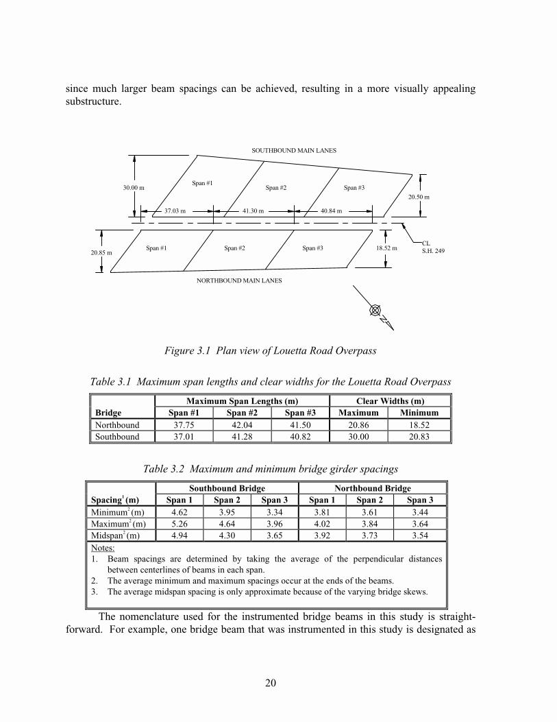
20
since much larger beam spacings can be achieved, resulting in a more visually appealingsubstructure.
�������
������� ������� ������
������
����������
�
�������
�������������
������� ������ �������
�������
���������������� ����
���������������� ����
Figure 3.1 Plan view of Louetta Road Overpass
Table 3.1 Maximum span lengths and clear widths for the Louetta Road Overpass
Maximum Span Lengths (m) Clear Widths (m)Bridge Span #1 Span #2 Span #3 Maximum MinimumNorthbound 37.75 42.04 41.50 20.86 18.52Southbound 37.01 41.28 40.82 30.00 20.83
Table 3.2 Maximum and minimum bridge girder spacings
Southbound Bridge Northbound BridgeSpacing1 (m) Span 1 Span 2 Span 3 Span 1 Span 2 Span 3Minimum2 (m) 4.62 3.95 3.34 3.81 3.61 3.44Maximum2 (m) 5.26 4.64 3.96 4.02 3.84 3.64Midspan2 (m) 4.94 4.30 3.65 3.92 3.73 3.54Notes:1.� Beam spacings are determined by taking the average of the perpendicular distances
between centerlines of beams in each span.2.� The average minimum and maximum spacings occur at the ends of the beams.3.� The average midspan spacing is only approximate because of the varying bridge skews.
The nomenclature used for the instrumented bridge beams in this study is straight-forward. For example, one bridge beam that was instrumented in this study is designated as

21
S14. The first letter in the beam designation tells where it is located. The location of a beamwill be in either the southbound main lane (S) or northbound main lane (N) bridge. Thesecond label identifies the span in which the beam is located. For this example, Beam S14 islocated in the first span of the southbound bridge. The third label tells exactly which lateralposition that beam occupies in its particular span. Beam S14 is the fourth beam in the spanwhere beam one corresponds to the west exterior girder. Figures 3.2 and 3.3 show the beamnomenclature system for each bridge. The darkened beam locations identify the twelvebeams that were instrumented for this study.
�
�
�
�
�����
�����
�� �
� ���������
�!���"#�!�$%&��'
�!�%���
�()%����
�!�%��
�()%����
Figure 3.2 Instrumented beams in the southbound main lanes bridge
� ���������
�
�
�
�� ���
���
�� ���
�()%�����!�%����!�%���()%����
�!���"#�!�$%&��'
Figure 3.3 Instrumented beams in the northbound main lanes bridge

22
3.2.2 Bridge Girder Details
As previously mentioned, the Louetta Road Overpass was designed using the newlydeveloped Texas U-beam. As indicated by Ralls et al. (1), the Texas U-beam cross sectionwas developed with a renewed focus on aesthetics while emphasizing the need for theeconomical, durable, and functional qualities that are inherent to structures constructed usingthe standard I-shaped beams. The aesthetic advantages of the U-beam are apparent fromconsideration of the shape and spacing of the girder. The standard AASHTO I-shapedgirders have several horizontal break lines on their web faces. The trapezoidal shape of the U-beam eliminates those visual breaklines and gives the bridge smoother lines. Larger beamspacing can be achieved with the Type U54 beam because it has nearly twice the moment ofinertia as the AASHTO Type IV girder. The larger spacing will result in a more open andattractive superstructure. It will also create more options for the substructure, such as beamsbeing supported on individual piers, as is the case in this project.
While the transportation and fabrication costs of the U-beam exceed those of thestandard I-shaped girders, several economical advantages can be realized with the U-beam(1). One advantage is that fewer beams per span are needed to complete a bridgesuperstructure. This may result in savings in material, transportation, and fabrication costsfor the whole project. Additionally, longer spans and larger spacing can be achieved with theU-beam. When combined with high performance materials, such as high strength concreteand 15.2 mm-diameter prestressing strand, the advantage of longer spans will result in areduction in the number of substructure units. Russell (3) points out that a cost savings canbe realized with high strength concrete U-beams when shallower superstructures can be usedfor longer spans. The savings resulting from shallower sections will come from reductions inpier, abutment, and approach work costs. The practical limitations imposed on span length,such as girder self-weight and difficulty in transportation and handling of very long beams,indicate that the greatest advantage may come from larger beam spacing and shallowersections.
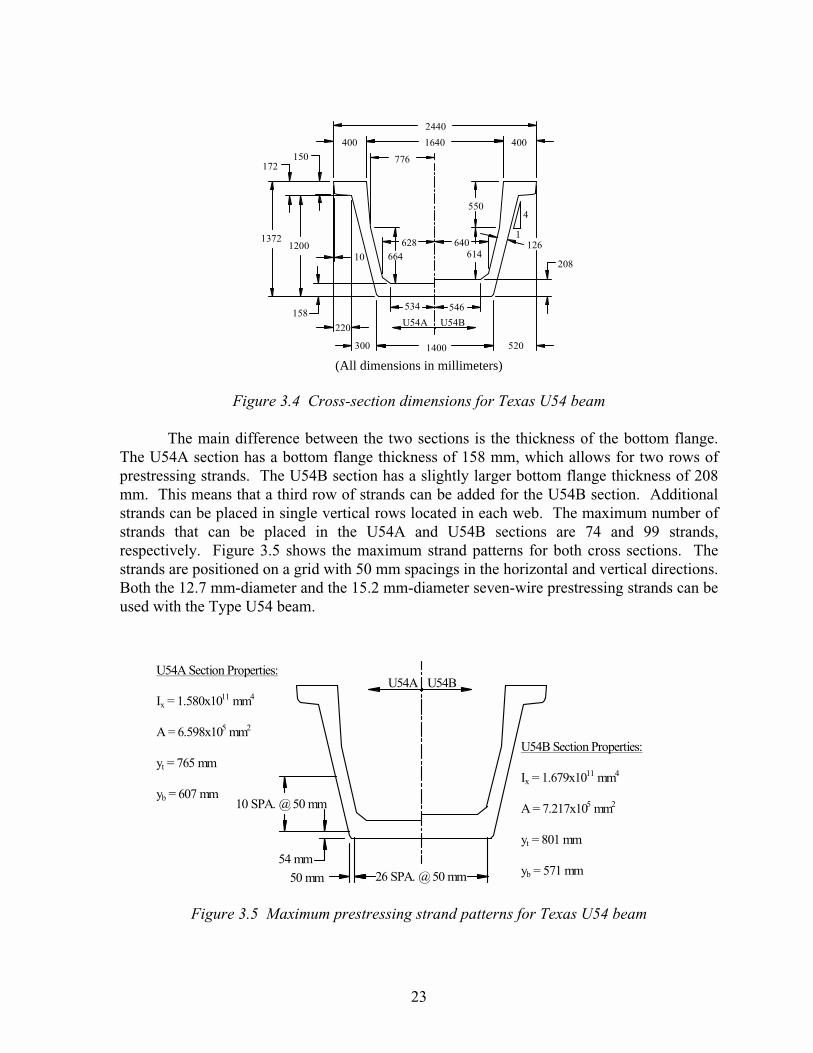
The cross-sectional dimensions of the U54A and U54B girders are shown in Figure3.4. These sections were developed in metric units to comply with the Federal HighwayAdministration (FHWA) initiative that all federally funded projects have constructiondocuments that are produced using the International System of units (metric system) bySeptember of 1996 (1). Both of these sections were used in the Louetta Road Overpass andboth were included as part of the twelve instrumented beams in this research study.
At first glance the U54A and U54B cross sections look identical. Both sections havean overall top width of 2440 mm, two top flanges that are 400 mm wide and 150 mm thick,and a bottom flange width of 1400 mm. The Type U54 beam is 1372 mm deep, matching thedepth of the AASHTO Type IV beam. The reason for this was to allow for widening ofexisting I-shaped girder bridges with the more visually appealing Type U54. There are twowebs in the Type U54 beam, each with a width of 126 mm. The outside web faces taperdownwards at a 4-to-1 slope, as shown in Figure 3.4, resulting in the attractive trapezoidalshape.
23
���
� ��
��
������
�
��
�
��
� ��
���
���� ����
��� ��
�����
�
��
�����
������
��
����
(All dimensions in millimeters)
Figure 3.4 Cross-section dimensions for Texas U54 beam
The main difference between the two sections is the thickness of the bottom flange.The U54A section has a bottom flange thickness of 158 mm, which allows for two rows ofprestressing strands. The U54B section has a slightly larger bottom flange thickness of 208mm. This means that a third row of strands can be added for the U54B section. Additionalstrands can be placed in single vertical rows located in each web. The maximum number ofstrands that can be placed in the U54A and U54B sections are 74 and 99 strands,respectively. Figure 3.5 shows the maximum strand patterns for both cross sections. Thestrands are positioned on a grid with 50 mm spacings in the horizontal and vertical directions.Both the 12.7 mm-diameter and the 15.2 mm-diameter seven-wire prestressing strands can beused with the Type U54 beam.
������!*%#+��,-+�!-%#!./
�0�1��� ��0��������
��1�����0������
&%�1������
&(�1�������
���� ����
�����
�����
����,���2������
��,���2������
������!*%#+��,-+�!-%#!./
�0�1�����0��������
��1� ���0������
&%�1�� ����
&(�1� �����
Figure 3.5 Maximum prestressing strand patterns for Texas U54 beam

24
The U-beam also has two internal diaphragms that vary in thickness and are locatedapproximately 0.4L and 0.6L from one end of the beam. These diaphragms help to stiffenthe two separated webs. The beams also had solid end blocks which varied in thickness(minimum thickness of 457 mm) because of the bridge skew.
3.2.3 Composite Bridge Details and Support Conditions
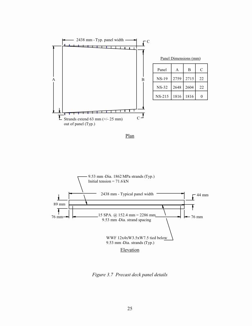
Both bridge superstructures in the Louetta Road Overpass were designed asprestressed concrete beam sections acting compositely with precast prestressed concrete deckpanels and a reinforced concrete deck cast over the panels. The details of the compositebridge section are shown in Figure 3.6. The composite deck was designed to be 184 mmthick. The thickness of the precast panels is 89 mm, and the thickness of the cast-in-placeslab is 95 mm. The use of precast panels in deck construction is just as advantageous withthe U-Beam bridge as it is with the I-shaped girder bridges. The precast panels make thedeck easier to construct because less formwork preparation is needed and contractorsfrequently select this option for Texas bridges. Figure 3.7 gives details and dimensions forthe precast deck panels.
�3!-�""�4#5%6�3�-#!.
� ����%�� �+7
(!�%
� ����%�� �+7
(!�%��+-���!8)�"�.��*!.�$*+--!.�+�5#�9�%+���-%#*)"�-�(-#59!'
� �(!����+��� � �(!��
�+����+-
�+�
�����0
������7#(!-:
(+�-5�.%-#�.
;#5%6�3�-#!.
(!%4!!��(!��.
��� ���%&��
+3!-�(!��.������*+3!-�%&����������!"
������5!*<�����
���(�-.�.�����%��������:
%&���%-��.3!-.!�5!*<�-!#�7�
���(�-.�.�����%��������:
%&���"+�9��5!*<�-!#�7�
Figure 3.6 Composite U-beam cross-section details
The beams in the Louetta Road Overpass were designed as simply supportedmembers. The typical support conditions for the U-beam can be seen in Figure 3.8. One endof the beam rested on a single bearing pad while the other end of the beam rested on twobearing pads. The bearing pad material was 50 durometer steel laminated neoprene. Thepads were of varying thickness and were beveled to allow the beam to conform to the gradeof the bridge.
25
�
�
�
�
,��!"��#�!�.#+�.�$��'
,��!" � � �
��:��
��:�
��:��
��� ���
� ��
�� �� �
������:��&������!"�4#5%6
�%-��5.�!0%!�5� �����$=>:�����'
+)%�+7����!"�$�&��'
Plan
� ��� � ���
�����
����
������:��&�#*�"����!"�4#5%6
��������:�#���� ��,��.%-��5.�$�&��'
��#%#�"�%!�.#+��1���� �<�
����,���2���������1� ���
��������:�#���.%-��5�.��*#�9
;;?��0�0;���0;����%#!5�(!"+4
��������:�#���.%-��5.�$�&��'
Elevation
Figure 3.7 Precast deck panel details

26
At Abutments (Typical)
Elevation
Figure 3.8 Typical bearing details for instrumented beams in both bridges
3.2.4 Instrumented Beams
Twelve Texas U54 beams were instrumented in the field for the purpose of measuringcamber and deflection, internal strains, and temperatures gradients over time through thevarious stages of fabrication and construction. The locations of the instrumented beams were
?�*!�+7�(�*<4�""
��#��%!5�(!�-#�9
��5$.'�$%&��'
� ����:��"+�9��
+7��:(!��
������:��!-�!�5#*)"�-�5#.%��*!
7-+��(�*<4�""�%+�� �(!�-#�9
�-��.3!-.!��
+7��#!-
��#��%!5�(!�-#�9
��5$.'�$%&��'
�����%+�� �+7�(!�-#�9
�"+�9�� �+7��:(!��
�����%+�� �+7�(!�-#�9
�"+�9�� �+7��:(!��
������:��"+�9�� �+7��:(!��
������:��"+�9�� �+7��:(!��

27
chosen to reflect the goals of the instrumentation plan. One of the goals of the project was todetermine the live load distribution factors for adjacent interior and exterior beams within thesame span. Another consideration was that the number of data acquisition systems used toread the instrumentation needed to be minimized. To satisfy these requirements, four groupsof three beams were chosen to be instrumented as shown in Figures 3.2 and 3.3. By groupingthe beams together in this manner, only two data acquisition boxes were needed to read all ofthe beam and deck gages.
An exterior beam was included in each of the four instrumented groups because theexterior beam typically had the most prestressing strands, and it would also have thermalgradients that were different from the interior beams.
The geometric and material properties of the instrumented beams are summarized inTable 3.3. There were four different strand patterns among the twelve instrumented U-beams. The number of 15.2 mm-diameter low relaxation prestressing strands in a particularbeam varied from a minimum of 64 to a maximum of 87, depending on where the beam waslocated in the bridge. The different strand patterns for the instrumented beams are shown inFigures 3.9 through 3.12. Both the U54A and U54B cross sections of the Texas U-beamwere included in the group of instrumented beams. The U54B section, which has a higherstrand capacity than the U54A section, was used for the exterior beams because those beamsrequired the most prestressing force.
765
mm
C.G.U.
607
mm
e =
507
mm
CGS = 100 mm
12.5 mm (typ)
26 SPA. @ 50 mm = 1300 mm 54 mm
5 SPA. @50 mm = 250 mm
Figure 3.9 Instrumented U-beam strand pattern – 64 strands

28
801
mm
C.G.U.
571
mm
e =
477
mm
CGS = 94 mm
12.5 mm (typ)
26 SPA. @ 50 mm = 1300 mm 54 mm
2 SPA. @50 mm =100 mm
Figure 3.10 Instrumented U-beam strand pattern – 68 strands
801
mm
C.G.U.
571
mm
e =
465
mm
CGS = 106 mm
12.5 mm (typ)
12 SPA. @ 50 mm = 1300 mm 54 mm
3 SPA. @50 mm =150 mm
Figure 3.11 Instrumented U-beam strand pattern – 83 strands

29
801
mm
C.G.U.
571
mm
e =
459
mm
CGS = 112 mm
12.5 mm (typ)
26 SPA. @ 50 mm = 1300 mm 54 mm
4 SPA. @50 mm =200 mm
Figure 3.12 Instrumented U-beam strand pattern – 87 strands
Figure 3.8: Typical bearing details for instrumented beams in both bridges
The design beam lengths, which are the lengths of the beams from end to end, variedfrom 35.94 meters for Beam S14 to 41.58 meters for Beam N23. In this study the length ofinterest was the span length, which was taken as the center-to-center of bearing length. Thislength was used for calculating camber and deflection predictions, which were used tocompare to the measured values. The center-to-center of bearing lengths varied from 35.55meters (S14) to 41.25 meters (N23).
The casting dates shown in Table 3.3 indicate that the first eight instrumented beamswere cast between September and November of 1994, while the remaining four beams werecast in February of 1996. This created an age difference of as much as 521 days betweenbeams in the first group and beams in the second group. The difference in age was importantwhen comparing the measured growth of camber during storage. Additionally, there werefour pairs of beams that were cast at the same time on the same stressing bed. This wasimportant for making comparisons of long-term behavior between the companion beams. Itwas also important because the internal temperature data from one beam could be used tocorrect the camber readings for thermally induced camber and deflection for both beams inthe pair.
3.3 INSTRUMENTATION
3.3.1 Selection of Instrumentation
The purpose of this study was to monitor the time-dependent behavior of a full-scalehighway bridge structure. To learn about the long-term behavior of high performanceconcrete in these bridges, three types of measurements needed to be obtained over a period ofseveral years.
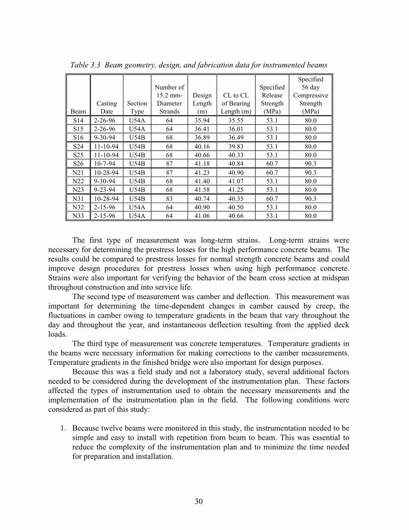
30
Table 3.3 Beam geometry, design, and fabrication data for instrumented beams
BeamCasting
DateSectionType
Number of15.2 mm-DiameterStrands
DesignLength
(m)
CL to CLof BearingLength (m)
SpecifiedReleaseStrength(MPa)
Specified56 day
CompressiveStrength(MPa)
S14 2-26-96 U54A 64 35.94 35.55 53.1 80.0S15 2-26-96 U54A 64 36.41 36.01 53.1 80.0S16 9-30-94 U54B 68 36.89 36.49 53.1 80.0S24 11-10-94 U54B 68 40.16 39.83 53.1 80.0S25 11-10-94 U54B 68 40.66 40.33 53.1 80.0S26 10-7-94 U54B 87 41.18 40.84 60.7 90.3N21 10-28-94 U54B 87 41.23 40.90 60.7 90.3N22 9-30-94 U54B 68 41.40 41.07 53.1 80.0N23 9-23-94 U54B 68 41.58 41.25 53.1 80.0N31 10-28-94 U54B 83 40.74 40.35 60.7 90.3N32 2-15-96 U54A 64 40.90 40.50 53.1 80.0N33 2-15-96 U54A 64 41.06 40.66 53.1 80.0
The first type of measurement was long-term strains. Long-term strains werenecessary for determining the prestress losses for the high performance concrete beams. Theresults could be compared to prestress losses for normal strength concrete beams and couldimprove design procedures for prestress losses when using high performance concrete.Strains were also important for verifying the behavior of the beam cross section at midspanthroughout construction and into service life.
The second type of measurement was camber and deflection. This measurement wasimportant for determining the time-dependent changes in camber caused by creep, thefluctuations in camber owing to temperature gradients in the beam that vary throughout theday and throughout the year, and instantaneous deflection resulting from the applied deckloads.
The third type of measurement was concrete temperatures. Temperature gradients inthe beams were necessary information for making corrections to the camber measurements.Temperature gradients in the finished bridge were also important for design purposes.
Because this was a field study and not a laboratory study, several additional factorsneeded to be considered during the development of the instrumentation plan. These factorsaffected the types of instrumentation used to obtain the necessary measurements and theimplementation of the instrumentation plan in the field. The following conditions wereconsidered as part of this study:
1.� Because twelve beams were monitored in this study, the instrumentation needed to besimple and easy to install with repetition from beam to beam. This was essential toreduce the complexity of the instrumentation plan and to minimize the time neededfor preparation and installation.

31
�
2.� The instrumentation needed to be durable because the field monitoring program wasgoing to begin at the time of fabrication of the beams and last several years into theservice life of the bridge. Another reason for durability was that any exposed portionsof the instrumentation would be subjected to harsh weather conditions and possibledamage during handling and transportation of the beams.
�
3.� Since there would be involvement with contractors throughout the entire study, itwould be important to establish a good working relationship between the researchersand the contractors. This relationship would require frequent communication so thatthe researchers could install and monitor the instrumentation without significantlydisrupting the fabrication and construction processes.
�
4.� Because the locations of the precast plants and project site were several hours oftravel from the laboratory in Austin, consideration was given to the amount of timethat would be lost during trips to and from these places. The extended travel timewould take away from the time needed for preparation, planning and building of theinstrumentation systems. Also, the distance from these sites would become veryimportant during coordination with the contractors for installation and monitoring ofthe instrumentation.
With these considerations in mind, along with the goals for this study, theinstrumentation systems were chosen and developed for the beams, deck panels and cast-in-place deck. The following sections describe exactly what types of instrumentation were usedto monitor the behavior of the structural components of the bridges and where they wereplaced in the various structural components.
3.3.2 Concrete Surface Strain Measurement
Concrete surface strain measurements were obtained through the use of a Demecmechanical strain gage. The gage consists of a dial mounted on a steel bar that has conicalshaped tips at each end underneath the gage. The tips of the gage fit neatly into the Demecpoints, which are specially fabricated stainless steel disks with conical holes in the center.One tip is allowed to move so that the distance between points can be translated into areading on the dial. The initial and final reading on the Demec gage for a set of pointsdetermines the change in length and consequently the strain between the points. Aconversion to strain needed to be made since the dial gage did not measure strain directly.The difference in gage readings multiplied by the strain per division for the gage gave thetotal strain between the set of points. For the gage used in this study, each division on thedial gage was equal to 8.1 microstrain. Figure 3.13 shows the Demec mechanical strain gageand stainless steel disks.

32
Figure 3.13 Demec surface strain measuring system
The procedure for using this system began with the placement of Demec points on thesurface of interest. Points were placed by using a spacer bar that was approximately 200millimeters in length, which corresponded to the gage length. The Demec points were fixedto the concrete surface with standard five-minute epoxy gel. Although this type of epoxy didnot have extremely long-term durability, its use was necessary to minimize the time loss forthe fabricator.
Initial readings were taken before the release of the prestressing force and subsequentreadings were taken after release. The total strain measured between the points included thethermally induced strains from the beam. The effects of temperature on the Demec gagecould be accounted for by measuring the standard invar bar for each set of readings. Surfacetemperatures needed to be measured to account for the thermally induced strain betweenreadings.
Previous research by Kelly et al. (26) showed that the five-minute epoxy hadreliability and durability problems when used to affix the mechanical strain gages to concretesurfaces. As a result, the use of mechanical strain gages were limited to transfer lengthreadings and backup readings for other internal instrumentation. The measurements ofinterest for this study were the strain measurements at the midspan to determine the sectionalbehavior after transfer of the prestressing force and the strain measurements at the CGS alongthe beam length. This type of instrumentation was fairly easy to install with little preparationtime and these measurements were taken in a short time period after transfer. Table 3.4summarizes the locations of the concrete surface strain instrumentation, and Figures 3.14 and3.15 show typical locations for instrumentation.

33
CG
U
Internal strain and temperatureinstrumentation (typ)
Steel ruler for tensioned piano wire camberand deflection measuring system
Demec surface straininstrumentation (typ)
Beam midspan
CG
C
CGS51 mm
1168
mm
1321
mm
Figure 3.14 Vertical locations for beam instrumentation at midspan
Intrumentation stations
Beam length (varies)
1
Quarter point
2 3 4 5 6 7
Midspan
Three-quarter point
0.61 m from end of beam (typical both ends)
1.22 m from CL bearing (typical both ends)
Figure 3.15 Horizontal locations for beam instrumentation
3.3.3 Internal Strain Measurement
Two types of internal strain measuring instrumentation were utilized to monitor thebehavior of the prestressed beams. The first type of instrumentation was the electricalresistance strain gage (ERSG). The ERSG measures strain based on a change in resistance.The change in resistance occurs as the small wires in the gage change length, or strain.Because this is a resistance-based measurement, the reliability of the readings can bequestionable owing to unwanted resistance. Resistance is added into the system asconnections are made to the lead wires and as various connections are made to the dataacquisition equipment.
Preparation of an ERSG for use consisted of bonding the gage to a piece of #3 rebar(approximately 1 meter long) that was specially prepared by grinding, sanding, and cleaningan area for the gage. Once the gage was bonded to the rebar, it was necessary to apply

34
waterproofing to the gage and lead connections to prevent moisture penetration. By bondingthe gage to the rebar, a simple and effective means of inserting the gage into the beam at thedesired location was established. The ERSG was an inexpensive alternative for gatheringshort-term strain measurements. The reliability and durability characteristics for this type ofgage limited the usefulness of its readings to approximately one year.
The ERSGs used in the cast-in-place decks were prepared differently than the onesused in the beams. Instead of bonding the gages to #3 rebar, they were bonded to 9.5 mm-diameter threaded rods that were 150 mm long. Using a grinder, flat surfaces were made inthe center of the rods. Large washers were mechanically fastened to the ends of the rods toprovide anchorage in the concrete. Then, the gages were bonded onto the flat surfaces andprotected with weather-proofing agents.
Table 3.4 Summary of external instrumentation for beams
BeamDemec SurfaceStrain Gages1
Tensioned Piano Wire Camber and DeflectionMeasuring System1
S14 midspan/both/all midspan/bothS15 midspan/both/all midspan/bothS16 midspan/both/all
along length/both/CGSmidspan/both
S24 midspan/bothS25 midspan/both/all
along length/both/CGSmidspan/both
S26 midspan/both/allalong length/both/CGS
midspan/both
N21 midspan/both/allalong length/both/CGS
midspan/both
N22 midspan/both/allalong length/both/CGS
midspan/both
N23 midspan/both/allalong length/both/CGS
midspan/both
N31 midspan/both/allalong length/both/CGS
midspan/both
N32 midspan/bothN33 midspan/both
Notes:1.� Descriptions of instrumentation locations consist of three parts. The first part gives the station
along the beam (along length refers to all of the stations shown in Fig. 3.15.). The second partgives the side(s) of the beam (east, west, or both). The third part tells the vertical location (CGSrefers to the center of gravity of the prestressing strands and all means every vertical positionsshown in Fig. 3.14.).
The second type of internal strain measuring instrumentation utilized in this studywas the vibrating wire (VW) gage manufactured by Roctest, Inc. The model EM-5 straingage is 168 mm in length and is composed of two circular end pieces joined by a stainlesssteel tube that contains a high tensile strength steel wire. The end pieces allow for the gage
35
to anchor into the concrete and transfer concrete deformation to the wire. Voltage pulses thatcause the wire to oscillate are sent to the wire from the coil/magnet assembly in the gage.Strain that develops in the concrete changes the tension of the wire, which changes itsresonant frequency. Thus, the change in resonant frequency of the wire is used to determinethe change in strain in the concrete.
There was very little preparation needed for the VW gages. Each gage was tied to apiece of #3 rebar (approximately 1 meter long) for later placement in the beam. The VWgages used in the precast deck panels and cast-in-place decks were not attached to a piece ofrebar, but simply tied directly onto the reinforcement in the field. Because of their strong anddurable outer shells, these gages were expected to last nearly three years. An additionalbenefit to the VW gage was that it had a thermistor for temperature measurement inside of acoil/magnet assembly. This was beneficial for determining thermal gradients within thebeam, which contributed to the camber of the beam. The one drawback to the VW gage wasthat it cost approximately 10 times that of an ERSG, which meant that a tradeoff in quantityand reliability needed to be determined.
The VW gages were utilized in the places where reliable long-term data were themost critical for this study. Since the prestress losses of the strands in the beams throughoutthe stages of construction was of great interest, six of the instrumented beams had a VW gageat the CGS on at least one side of the beam. In addition, there was an interest in the strainson the cross section at midspan throughout construction. Four of the instrumented beams hadVW gages throughout the depth of the cross section at midspan on at least one side of thebeam. To complete the vertical strain profile at midspan for two of the instrumented beams,VW gages were placed in the cast-in-place deck. Additional gages were placed in the precastdeck panels for determination of live load distribution factors for the completed bridge. TheERSGs were utilized mainly for strains immediately after transfer of prestressing force and toprovide redundancy at critical locations in the instrumented beams. Table 3.5 includes asummary of the internal strain measuring instrumentation for the twelve U-beams. Figures3.14 and 3.15 show the instrumentation locations in the beams. A summary of the internalstrain instrumentation for the precast deck panels is given in Table 3.6. Instrumentationplaced in the cast-in-place decks is summarized in Tables 3.7 and 3.8.
3.3.4 Internal Temperature Measurement
As mentioned in Sec. 3.3.3, one method of measuring the internal concretetemperature was with thermistors located inside the vibrating wire gages. The other methodemployed in this study was the use of thermocouples that were prepared by the researchers.The thermocouples were created by twisting a copper wire and a constantin wire together andcovering the connection with electrical tape. The wire and connectors were manufactured byOmega Engineering, Inc.

36
Table 3.5 Summary of internal instrumentation for beams
Beam
Electrical ResistanceStrain Gauges
(ERSG)2
Vibrating Wire Gauges(VW)2
InternalTemperature2
S14 midspan/east/all midspan/east/all
S15 midspan/both/all
S16 midspan/east/allalong length/both/CGS midspan/west/CGS
midspan/east/alldiaphragm/NE/all
S24
S25along length/both/CGS1
midspan/east/allmidspan/west/CGS
alonglength/east/CGS
S26 along length/east/CGS along length/west/CGS
N21 midspan/west/allalong length/both/CGS
midspan/both/all
N22 along length/both/CGS
N23 midspan/both/CGS
N31 along length/both/CGS
N32 midspan/east/all midspan/west/allmidspan/east/CGS
N33 midspan/east/all midspan/west/allmidspan/east/CGS
Notes:1.� Gages are placed along beam length at every station shown in Fig. 3.15 except midspan.2.� Descriptions of instrumentation locations consist of three parts. The first part gives the
station along the beam (along length refers to all of the stations shown in Fig. 3.15.). Thesecond part gives the side(s) of the beam (east, west, or both). The third part tells thevertical location (CGS refers to the center of gravity of the prestressing strands and all
means every vertical positions shown in Figure 3.14.).
The thermocouples were placed in locations that corresponded to strain gage locationsfor simplicity of installation and for uniformity in the instrumentation plan. Thethermocouples were installed in the field on the #3 rebars used for the strain gages and tied inplace with electrical tape. Additional thermocouples were placed in the cast-in-place deckand precast panels. These locations were needed to complete the temperature profile fromthe bottom flange of the beam to the top of the slab. Tables 3.5 through 3.8 summarize thelocations of the thermocouples in the beams, panels, and decks and Figure 3.14 shows theirlocations on the beam cross section.

37
Table 3.6 Instrumented precast deck panels in southbound main lanes bridge
InstrumentationPanelDesignation
Location in SB MainLanes Bridge Vibrating Wire Gages1 Thermocouples2
NS-19 Between Beams S14 andS15 at midspan
two (2) at center of panel two (2), one at center of panel andone 76 mm from edge of panel
NS-32 Between Beams S15 andS16 at midspan
two (2)at 305 mm fromtransverse edge3
two (2) at center of panel
NS-215 On top of Beam S15 atmidspan
two (2) at center of panel two (2) at center of panel
Notes:1.� Vibrating wire gages were tied across the strands at 38 mm above the bottom of the panel and parallel to the
strands at 51 mm above the bottom of the panel.2.� Thermocouples were prepared on a small piece of #2 bar to be able to position them at the vertical locations of
25 mm and 76 mm above the bottom of the panel.3.� These gages were positioned off the wrong edge of the panel. Section 4.5.1 discusses this in detail.
Table 3.7 CIP deck instrumentation for the southbound main lanes bridge
TransverseSection1 Beam2 Location3
GageType
Distance BelowPanel Surface (mm)4 Orientation5
Midspan of S14 E TC -44 ---Beam S14 TC 44 ---
S14 E ERSG 32 TW VW -38 L
VW 44 LERSG 38 T
P VW 64 LVW 38 T
S15 TC 51 ---Midspan of TC 13 ---Beam S15 E VW -32 T
VW 57 LERSG 38 T
S14/S15 P VW 38 TP VW 38 T
S15/S16 TC 51 ---TC 13 ---
S16 W ERSG 25 TMidspan of S16 E TC -44 ---Beam S16 TC 44 ---Midspan of S25 W VW 44 LBeam S25 E VW 51 L
VW -38 LAbut. No. 1 S15 W VW 51 L
E VW 57 LBent No. 2 S15 W VW 44 L
E VW 51 LBent No. 3 S25 W VW 51 L
E VW 44 L(Notes on following page.)

38
Notes:1.� A transverse section extends perpendicular to the specified beam. When a support location is given, the section
is only at the beam given in the next column.2.� S14/S15 and S15/S16 signify that the instrumentation is between beams.3.� Locations are the West (W) and East (E) top flange of the beam and over the panel (P).4.� Distances were measured in the field after gage installation.5.� Orientations of the gages were either longitudinal (L) or transverse (T) to the beams.6.� TC = Thermocouple; VW = Vibrating Wire Gage; ERSG = Electrical resistance strain gage.
Table 3.8 CIP deck instrumentation for the northbound main lanes bridge
TransverseSection1 Beam2 Location3
GageType
Distance Below CIPDeck Surface (mm)4 Orientation5
W ERSG 50 LN32 P ERSG 50 L
ERSG 50 TE ERSG 50 L
N32/N33 P ERSG 50 LMidspan of ERSG 50 TBeam N33 W ERSG 50 L
VW 50 LN33 VW 139 L
P ERSG 50 LERSG 50 T
E ERSG 50 LW ERSG 50 L
ERSG 50 TN32 P ERSG 50 L
ERSG 50 TE ERSG 50 L
ERSG 50 TMidspan of N32/N33 P ERSG 50 LBeam N32 ERSG 50 T
W ERSG 50 LERSG 50 T
N32 P ERSG 50 LERSG 50 T
E ERSG 50 LERSG 50 T
Midspan of W TC 50 ---Beam N21 N21 TC 139 ---
E TC 50 ---TC 139 ---
Notes:1.� A transverse section extends perpendicular to the specified beam.2.� N32/N33 signifies that the instrumentation is between beams.3.� Locations are the West (W) and East (E) top flange of the beam and over the panel (P).4.� Distances were not measured in the field but approximated based on deck reinforcement.5.� Orientations of the gages were either longitudinal (L) or transverse (T) to the beams.6.� TC = Thermocouple; VW = Vibrating Wire Gage; ERSG = Electrical resistance strain gage.
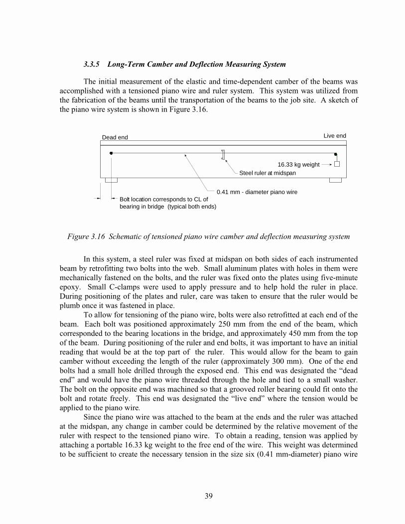
39
3.3.5 Long-Term Camber and Deflection Measuring System
The initial measurement of the elastic and time-dependent camber of the beams wasaccomplished with a tensioned piano wire and ruler system. This system was utilized fromthe fabrication of the beams until the transportation of the beams to the job site. A sketch ofthe piano wire system is shown in Figure 3.16.
Steel ruler at midspan16.33 kg weight
Live endDead end
0.41 mm - diameter piano wireBolt location corresponds to CL ofbearing in bridge (typical both ends)
Figure 3.16 Schematic of tensioned piano wire camber and deflection measuring system
In this system, a steel ruler was fixed at midspan on both sides of each instrumentedbeam by retrofitting two bolts into the web. Small aluminum plates with holes in them weremechanically fastened on the bolts, and the ruler was fixed onto the plates using five-minuteepoxy. Small C-clamps were used to apply pressure and to help hold the ruler in place.During positioning of the plates and ruler, care was taken to ensure that the ruler would beplumb once it was fastened in place.
To allow for tensioning of the piano wire, bolts were also retrofitted at each end of thebeam. Each bolt was positioned approximately 250 mm from the end of the beam, whichcorresponded to the bearing locations in the bridge, and approximately 450 mm from the topof the beam. During positioning of the ruler and end bolts, it was important to have an initialreading that would be at the top part of the ruler. This would allow for the beam to gaincamber without exceeding the length of the ruler (approximately 300 mm). One of the endbolts had a small hole drilled through the exposed end. This end was designated the “deadend” and would have the piano wire threaded through the hole and tied to a small washer.The bolt on the opposite end was machined so that a grooved roller bearing could fit onto thebolt and rotate freely. This end was designated the “live end” where the tension would beapplied to the piano wire.
Since the piano wire was attached to the beam at the ends and the ruler was attachedat the midspan, any change in camber could be determined by the relative movement of theruler with respect to the tensioned piano wire. To obtain a reading, tension was applied byattaching a portable 16.33 kg weight to the free end of the wire. This weight was determinedto be sufficient to create the necessary tension in the size six (0.41 mm-diameter) piano wire

40
that was used for this system. A loop tied at the free end of the wire was hooked onto theweight, and the piano wire was placed in the machined groove on the outside surface of thebearing. The weight was slowly lowered until the piano wire and weight reached equilibrium.Finally, a reading was taken on the ruler at midspan. A small mirror was placed behind theruler and wire to eliminate parallax during the reading. To determine the camber of thebeam, the reading needed to be compared to the initial reading that was taken just beforerelease of the prestressing force. The accuracy of the rulers in this system were 0.01 inches.This accuracy is equivalent to approximately 0.25 mm.
Once the beams were transported to the job site, the tensioned piano wire systemcould no longer be utilized. Section 4.3.1 describes several reasons why the system failed atthat point. A precise surveying system was employed in which beam elevations weremeasured at the supports and at the midspan of each beam using a level and rod.
Figure 3.17 shows a picture of the researchers measuring beam elevations with thissystem. To obtain accurate readings, the level needed to be very close to the rod and therulers used in the original system needed to be fastened to the rod. Paint markings wereplaced on the underside of the beams to locate the surveying points. Readings under thissystem were read to 0.02 inch accuracy on the ruler, which is equivalent to approximately0.51 mm. This system worked well and had acceptable repeatability. Some of thedifficulties encountered while using this system are described in Sec. 4.5.
Figure 3.17 Precise surveying system for measuring beam camber
3.4 DATA ACQUISITION
3.4.1 General
The method of data acquisition chosen for this study was an automated system thatcould handle the readings from dozens of gages at frequent time intervals. This was anecessary aspect of the data acquisition system because of the complexity and size of theinstrumentation plan. Although the automated system was more costly and requiredsignificant time and labor in preparation, the savings in work in the field and during data
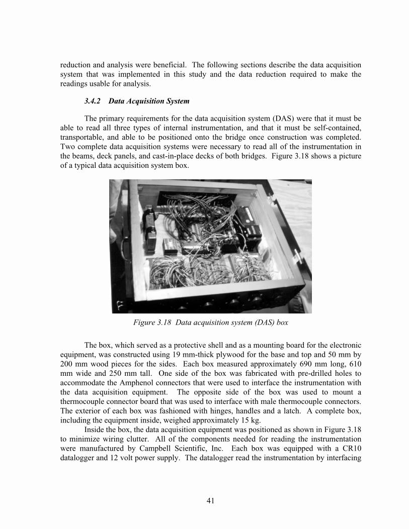
41
reduction and analysis were beneficial. The following sections describe the data acquisitionsystem that was implemented in this study and the data reduction required to make thereadings usable for analysis.
3.4.2 Data Acquisition System
The primary requirements for the data acquisition system (DAS) were that it must beable to read all three types of internal instrumentation, and that it must be self-contained,transportable, and able to be positioned onto the bridge once construction was completed.Two complete data acquisition systems were necessary to read all of the instrumentation inthe beams, deck panels, and cast-in-place decks of both bridges. Figure 3.18 shows a pictureof a typical data acquisition system box.
Figure 3.18 Data acquisition system (DAS) box
The box, which served as a protective shell and as a mounting board for the electronicequipment, was constructed using 19 mm-thick plywood for the base and top and 50 mm by200 mm wood pieces for the sides. Each box measured approximately 690 mm long, 610mm wide and 250 mm tall. One side of the box was fabricated with pre-drilled holes toaccommodate the Amphenol connectors that were used to interface the instrumentation withthe data acquisition equipment. The opposite side of the box was used to mount athermocouple connector board that was used to interface with male thermocouple connectors.The exterior of each box was fashioned with hinges, handles and a latch. A complete box,including the equipment inside, weighed approximately 15 kg.
Inside the box, the data acquisition equipment was positioned as shown in Figure 3.18to minimize wiring clutter. All of the components needed for reading the instrumentationwere manufactured by Campbell Scientific, Inc. Each box was equipped with a CR10datalogger and 12 volt power supply. The datalogger read the instrumentation by interfacing

42
with AM416 relay multiplexers. The multiplexers were wired into the Amphenol connectorson the side of the box. The number of multiplexers in a box depended upon the amounts ofeach type of instrumentation in the particular bridge. Storage modules were used to hold theprogramming for the CR10 and to hold the data from the instrumentation. A keypad wasused as an interface with the CR10 and was connected in series with the datalogger andstorage module. The storage modules could be connected to a personal computer fordownloading data as well as further programming.
3.4.3 Data Reduction
The raw measurements from the instrumentation and the date and time data were allin voltages. The program in the storage module was only set up to change the temperatureinstrumentation readings from voltages to temperatures and the rest of the data was convertedusing a short program written for use on an IBM compatible personal computer. To convertthe strain instrumentation data, the initial readings of the instrumentation were needed. Datawas downloaded from the storage module into the personal computer and input into theprogram. The program also sorted the raw data files and arranged new data files so that theycould be inserted into a spreadsheet.
An option for data transfer which was not employed by the researchers was the use ofa modem to send the data directly from the DAS boxes to the personal computer. Since theDAS box was being moved to several locations before construction of the bridges, theindependent power supply and storage modules were a good system. The advantage of themodem would be realized once the DAS boxes were fixed permanently on the bridges.However, changing systems would not have been efficient, and the periodic switching ofstorage modules and batteries in the boxes was not difficult.
Once the data was put into a useful form, additional factors needed to be consideredbefore that data could be compared to analytical predictions. Thermal gradients within thebeam are created as a result of changes in external temperature conditions throughout the dayand throughout the year. The thermal gradients induce differential strain on the cross sectionof the beam and cause additional curvature in the beam, which affects the camber readings.This needed to be taken into account to calculate the actual camber of the beam. The internaltemperature instrumentation provided the information to make this correction.
The support conditions of the beams needed to be carefully recorded when takingmeasurements otherwise the data would have little meaning. After the beams were lifted offthe prestressing bed, they were stored in the yard on wooden railroad ties. The supportlocations were usually 0.5 to 1.0 meters in from the beam ends and did not correspond to thebearing locations in the bridge. Many of the beams cast in 1994 were moved in the yardseveral times and the support locations moved as well. The data needed to be adjusted forthese varying support conditions so that an accurate comparison of beam camber could bemade based upon the span length from bearing to bearing in the bridge.
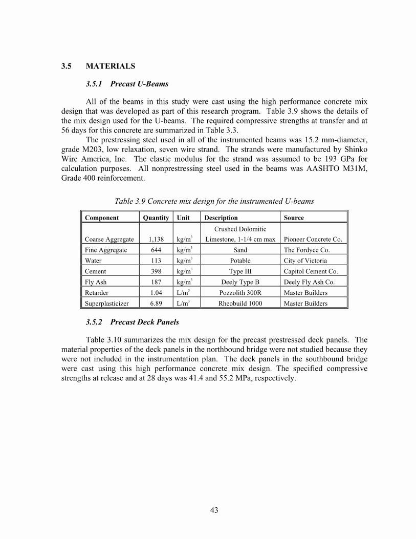
43
3.5 MATERIALS
3.5.1 Precast U-Beams
All of the beams in this study were cast using the high performance concrete mixdesign that was developed as part of this research program. Table 3.9 shows the details ofthe mix design used for the U-beams. The required compressive strengths at transfer and at56 days for this concrete are summarized in Table 3.3.
The prestressing steel used in all of the instrumented beams was 15.2 mm-diameter,grade M203, low relaxation, seven wire strand. The strands were manufactured by ShinkoWire America, Inc. The elastic modulus for the strand was assumed to be 193 GPa forcalculation purposes. All nonprestressing steel used in the beams was AASHTO M31M,Grade 400 reinforcement.
Table 3.9 Concrete mix design for the instrumented U-beams
Component Quantity Unit Description Source
Coarse Aggregate 1,138 kg/m3
Crushed Dolomitic
Limestone, 1-1/4 cm max Pioneer Concrete Co.
Fine Aggregate 644 kg/m3 Sand The Fordyce Co.
Water 113 kg/m3 Potable City of Victoria
Cement 398 kg/m3 Type III Capitol Cement Co.
Fly Ash 187 kg/m3 Deely Type B Deely Fly Ash Co.
Retarder 1.04 L/m3 Pozzolith 300R Master Builders
Superplasticizer 6.89 L/m3 Rheobuild 1000 Master Builders
3.5.2 Precast Deck Panels
Table 3.10 summarizes the mix design for the precast prestressed deck panels. Thematerial properties of the deck panels in the northbound bridge were not studied because theywere not included in the instrumentation plan. The deck panels in the southbound bridgewere cast using this high performance concrete mix design. The specified compressivestrengths at release and at 28 days was 41.4 and 55.2 MPa, respectively.

44
Table 3.10 Concrete mix design for the precast deck panels
Component Quantity Unit Description Source
Coarse Aggregate 1176 kg/m3
Crushed River Gravel,
19 mm max.
Fine Aggregate 659 kg/m3 Sand The Fordyce Co.
Water 135 kg/m3 Potable City of Houston
Cement 335 kg/m3 Alamo Type III Capitol Cement Co.
Fly Ash 97 kg/m3 Class C JTM
Retarder 0.85 L/m3 Pozzolith 300R Master Builders
Superplasticizer 6.24 L/m3 Rheobuild 1000 Master Builders
3.5.3 Cast-in-Place Deck Slabs
The deck slab for the southbound bridge was cast with a high strength, highperformance concrete mix. The specified 28-day design strength for cast-in-place decks forthe southbound bridge was 55.2 MPa. Table 3.11 summarizes the concrete mix design forthe cast-in-place deck in the southbound bridge.
The deck slab for the northbound bridge was cast with a normal-strength highperformance concrete mix that had a specified 28-day design strength of 27.6 MPa. Table3.12 summarizes the concrete mix design for the cast-in-place deck in the northbound bridge.
3.6 COMPANION TESTS
3.6.1 General
Several laboratory tests were performed on concrete cylinders made from the concreteused to cast the instrumented beams, panels and cast-in-place deck. These tests determinedthe properties of the high performance concretes that were necessary for making analyticalpredictions of the long-term behavior of the prestressed concrete U-beams and of thecomposite bridge section. Most of the concrete cylinders used for the tests were the smaller100 mm diameter by 200 mm tall specimens. The main reason for the smaller specimens wasto reduce the compressive force necessary to test the high strength concrete mixes. Thespecimens were cured under varying conditions, including match-cured using the internaltemperatures of the members, member-cured, and moist-cured following ASTMspecifications.

45
Table 3.11 Concrete mix design for the southbound main lanes bridge CIP deck
Component Quantity Unit Description SourceCoarse Aggregate 1074 kg/m3 Southwest Texas
Limestone, 19 mm max.Fine Aggregate 772 kg/m3 Sand The Fordyce Co.Water 146 kg/m3 Potable City of HoustonCement 281 kg/m3 Hunter Type IFly Ash 131 kg/m3 Class C JTMRetarder 0.85 L/m3 Pozzolith 300R Master BuildersSuperplasticizer 16.15 L/m3 Rheobuild 1000 Master Builders
Table 3.12 Concrete mix design for the northbound main lanes bridge CIP deck
Component Quantity Unit Description Source
Coarse Aggregate 1101 kg/m3Southwest Texas
Limestone, 19 mm max.Fine Aggregate 737 kg/m3 Sand The Fordyce Co.Water 136 kg/m3 Potable City of HoustonCement 230 kg/m3 Hunter Type IFly Ash 89 kg/m3 Class C JTMRetarder 0.85 L/m3 Masterpave ‘R’ Master Builders
3.6.2 Modulus of Elasticity
Concrete stress-strain tests were performed in accordance with ASTM C469-81 (50)on 100 mm by 200 mm specimens. A compressometer which satisfied ASTM C469-81requirements and which fit onto the smaller specimens was used to measure the strain.Concrete elastic moduli were found based upon the results of the tests. Specimens from allof the relevant beam, panel, and deck pours were tested at 1 day and at 28 days. Thespecimens from the two beam pours in 1996 were also tested at 7 days and 56 days.
3.6.3 Compressive Strength
Compressive strength tests were performed in accordance with ASTM C39-83b (51)on 100 mm by 200 mm specimens. The specimens were tested at the same ages as the elasticmodulus specimens. Results from these tests were used to construct age-strength gain curvesfor the different concrete mixes. This type of curve was of special interest for the prestressedbeams because of the very high release strengths that were required in the beam designs.

46
3.6.4 Creep and Shrinkage
Creep and shrinkage tests were performed on 100 mm by 600 mm specimensspecially fabricated using PVC pipe sections sealed on one end with aluminum disks. Thecreep tests conform to the specifications of ASTM C512 (52). All of the tests wereperformed in the Austin, Texas laboratory in a room without temperature or humidity control.This was the best attempt at simulating the actual environment of the beam, panel, and deckconcretes.
Figure 3.19 shows a picture of a typical creep test frame. Load was applied to acylinder by means of a hydraulic ram and a load cell. The springs and plates in the systemlock the applied load onto the specimen. Periodic re-application of the desired level of loadwas required as the specimen deformed over time. Indication of when to re-apply the loadwas obtained by monitoring the deformation of the springs. Strains in the concrete weremeasured using the Demec mechanical strain gage. Strains in several unloaded specimenswere also measured to determine the shrinkage portion of the deformation in the creepspecimens. Records were kept for the cylinder temperature, ambient temperature, andhumidity so that the data could be thermally compensated. A detailed description of the stepsfor specimen preparation and testing can be found in a report by Farrington et al. (8).
Farrington et al. (8) performed much of the testing on the beam mix design. His workincluded variables such as age of loading, magnitude of loading, and temperature of curing.Since Farrington only monitored the specimens up to an age of 120 days, the researchers ofthis study continued monitoring the specimens through the beginning of service life of thebridge. Additional tests were performed by the researchers on the precast panel mix designand both cast-in-place deck mix designs. The testing procedures were the same as those usedfor the beam specimens. The panel and deck creep specimens were loaded at 2 days to 20percent and 40 percent of the specified 28-day compressive strength. Readings were taken onshrinkage specimens at the same time as the creep specimens.
Figure 3.19 Creep test specimens sustaining applied load
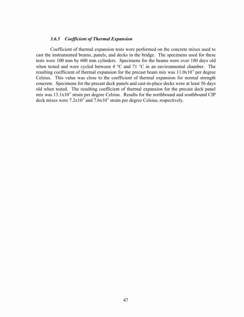
47
3.6.5 Coefficient of Thermal Expansion
Coefficient of thermal expansion tests were performed on the concrete mixes used tocast the instrumented beams, panels, and decks in the bridge. The specimens used for thesetests were 100 mm by 600 mm cylinders. Specimens for the beams were over 180 days oldwhen tested and were cycled between 4 �C and 71 �C in an environmental chamber. Theresulting coefficient of thermal expansion for the precast beam mix was 11.0x10⁻⁶ per degreeCelsius. This value was close to the coefficient of thermal expansion for normal strengthconcrete. Specimens for the precast deck panels and cast-in-place decks were at least 56 daysold when tested. The resulting coefficient of thermal expansion for the precast deck panelmix was 13.1x10⁻⁶ strain per degree Celsius. Results for the northbound and southbound CIPdeck mixes were 7.2x10⁻⁶ and 7.6x10⁻⁶ strain per degree Celsius, respectively.

48

49
CHAPTER 4. FIELD WORK
4.1 INTRODUCTION
4.1.1 Coordination with Contractors
While proper preparation of the instrumentation plan was necessary to obtain therequired data for long-term prestress loss, section behavior, and camber and deflection, anequally necessary and challenging aspect of this study was coordination with the contractorsduring the implementation of the instrumentation plan. One of the challenges was to conveythe importance of the research to the contractors while keeping in mind that their primaryinterest was in operating profitable businesses. Additional challenges included timemanagement for traveling and instrumentation preparation, dealing with unforeseen problemsin the field, and being flexible enough to adapt to the contractors’ schedules as much aspossible. The latter aspect helped to establish a favorable working relationship between theresearchers and the contractors.
Cooperation and coordination with Texas Concrete Company, which fabricated theprecast U-beams, was not a problem. Being one of the first prestressing plants to deal withhigh performance concrete for beam production, Texas Concrete was very helpful to theresearchers during all stages of the beam fabrication, instrumentation, and monitoring.Further work with Houston Prestress Products, Inc., during instrumentation of the precastdeck panels was satisfactory as well. Williams Brothers, Inc., was helpful at the job site,providing a man lift for use during installation of the data acquisition system (DAS) boxes inthe bridge, during connection of the gages to the DAS boxes, and during further accession ofthe DAS boxes to retrieve data.
4.1.2 Chapter Format
This chapter’s organization reflects the chronological order of the fabrication andconstruction of the bridges. It summarizes the field operations that were an important part ofthis research study. Initial comments are given on the procedures used to prepare theinstrumentation for installation in the field. Fabrication and instrumentation procedures forthe beams, deck panels, and cast-in-place decks are described. The chapter concludes with asection describing some of the problems encountered during the instrumentation installationand monitoring activities.
4.2 PREPARATION OF INSTRUMENTATION
When specific dates were established for a beam, panel, or deck slab pour, it wasimmediately necessary to review the instrumentation plan and prepare the gages that wouldbe installed. The typical preparation included the following:
1.� Prepare the various gages as described in Sec. 3.3.2.� Prepare lead wire for the gages. This step included spooling out, cutting, and
bundling lead wire for groups of gages. The grouping of gages to a specific

50
connector was done in the instrumentation plan. The length of lead wire wasimportant because the connectors needed to reach the DAS box location on thebridge.
3.� Attach the gages to the bundled lead wires.4.� Attach the connector to the bundled lead wires.5.� Gather the necessary equipment for the tensioned piano wire system (beams only).
During the instrumentation of the beams that were cast in 1994, the lead wires weresimply bundled together for transportation. Problems were encountered as the wires, whichsometimes exceeded 30 meters in length, became tangled, making installation cumbersome.Experience with those pours indicated that a more efficient means of gathering the massiveamounts of lead wire was needed to speed up installation and minimize delays to thecontractor. A spooling system for lead wires for transportation to the site was developed in1996 in response to that problem. Figure 4.1 shows a picture of the spooling system.
Figure 4.1 Spooling system used to gather gage lead wires
The spools were constructed from plywood and used to gather up the lead wire after itwas measured out, cut, and bundled. A wooden A-frame with steel hooks on the top wasused to operate the spooling system. A broomstick was used to spin the spool on the stand.The gages were connected to the appropriate wire ends so that the spools could be unwoundagain at the site. This system saved time during preparation, transportation, and installation.

51
4.3 PRECAST OPERATIONS
4.3.1 Precast Beams
All twelve of the instrumented beams were cast at the Texas Concrete Companyprestressing plant in Victoria, Texas. Eight of the beams were cast in late 1994 while theremaining four beams were cast in early 1996. The beam pours were arranged so that nomore than two of the instrumented beams were cast during the same pour. This reduceddelays for the fabricator and also eased the burden on the researchers. Nine pours wereneeded to fabricate all of the beams that were part of this study. The histories for all of theinstrumented beams are shown in Tables 4.1 and 4.2.
Table 4.1 Southbound main lanes bridge beam histories
Time from Casting (Days)Event S14 S15 S16 S24 S25 S26Casting completed 0 0 0 0 0 0Initial instrumentationmeasurement taken 1.19 1.19 1.12 1.14 1.10 7.05Transfer of prestressing force 1.30 1.30 1.18 1.19 1.15 7.11Beam moved to storage location 1.32 1.32 2.96 1.22 1.17 7.19Beam shipped to and placed inbridge 150 150 664 623 623 657Panels placed on beam 211 211 725 684 684 718Casting of deck slab 256 256 770 729 729 763
Table 4.2 Northbound main lanes bridge beam histories
Time from Casting (Days)Event N21 N22 N23 N31 N32 N33Casting completed 0 0 0 0 0 0Initial instrumentationmeasurement taken 1.16 1.03 0.99 1.20 1.29 1.29Transfer of prestressing force 1.22 1.09 1.03 1.28 1.35 1.35Beam moved to storage location 2.90 2.88 2.86 3.04 1.38 1.38Beam shipped to and placed inbridge 636 664 671 636 161 161Panels placed on beam 697 727 734 712 245 245Casting of deck slab 734 762 769 734 259 259
All of the U-beams were cast on the same bed. The bed was sufficiently long to castthree beams in one pour. This casting bed needed to be upgraded to a capacity of nearly 17.8MN to handle the design prestressing force for the U-beams. In addition, the stressinghardware needed to be retooled to handle this capacity.

52
The stressing operation was typically done two to three days before casting. Thestrands were pulled down the bed from the fixed end abutment to the stressing end with afork lift and were hand-threaded through the steel header forms, which were located at bothends of each beam. The strands were then hand-threaded through the stressing plate at the“live” or stressing end. The stressing end consisted of a stressing plate attached to a reactionplate with large diameter rods. Because the larger 15.2-mm diameter strands were used,special chuck placement was needed for the stressing operation. Spacers were placedbetween the stressing plate and the chucks so that they would fit in the 50 mm grid spacing ofthe strands. After the chucks were secured, the multi-strand stressing commenced. Thestressing plate was pulled forward as the hydraulic jacks pushed against the abutments andreaction plate. The stressing ended when the proper elongation of the strands was reached.This was determined based on the initial design stress of 1396 MPa, which is seventy-fivepercent of the specified strand strength.
Once the strand pattern was in place and stressed, strand debonding was applied withsplit plastic tubing. Where debonding was specified by design, the tubing was cut to properlength before being slipped over the strands and sealed with tape to prevent intrusion of theconcrete paste during casting. Appendix A contains the debonding details for theinstrumented beams.
After completing the stressing and debonding of the strands, the reinforcing steel wasplaced and tied. Much of the mild reinforcement consisted of welded-wire fabric and pre-tiedcages. Once the steel was tied in place, the internal strain gages and thermocouples wereattached to the strands or the stirrups at the required vertical and horizontal locations usingrebar ties. Figure 4.2 shows an internal strain gages installed in a beam. Once all of thegages were tied in on one side of the beam, the lead wire was secured to the reinforcementwith nylon cable ties. In an attempt to avoid damage from mechanical vibration of theconcrete during casting, the lead wires were run up to the top flange at their horizontallocation and tied along the top flange to the end of the beam.
Figure 4.2 Internal instrumentation placed at midspan of a beam

53
Next, the forms were placed in preparation for casting. Fork lifts with spreader barswere used to position the multiple side-form sections. These sections were bolted togetherand attached to the header forms that were placed before the stressing operation. Opposingside forms were connected with collars at the diaphragms to add rigidity. Finally, adjustable-length steel “tubs” were positioned as the internal void forms for the U-beams. These tubswere held in place by additional steel collars connected to the side forms.
Concrete placement followed shortly after the forms were positioned and secured.All of the high performance concrete was batched at the mixing plant and transported to thecasting bed in an auger bucket using a fork lift. The concrete was placed in the forms using adispensing unit coming from the auger bucket. It was imperative that the formation of voidsin the bottom flange was avoided during casting. To do this, the concrete, with a slump ofapproximately 200 mm, needed to be placed on one side of the beam and forced across thebottom flange and partially up the opposite web. Then, concrete was placed on the other sideof the beam to complete the casting. To ensure consolidation, external and internal vibrationwas used. This procedure was successful for all of the instrumented beams except BeamS26. After the forms were removed from Beam S26, voids were found in the bottom flangearound the strands and patching was necessary to cover up the exposed strands. This delayedthe transfer of prestress force for one week.
Once casting was completed, the beams were covered with tarps and allowed to cureto achieve the required release strength. Usually, it took only 24 to 27 hours to obtain thedesign release strength. After removal of the forms, the tensioned piano wire cambermeasurement system was installed on both sides of the beam. Also, researchers placed themechanical strain gages (Demec points) in their locations. The typical externalinstrumentation that was installed at midspan is shown in Figure 4.3. Just before transfer ofthe prestress force, an initial measurement was taken for all of the instrumentation. After theinitial measurements were gathered, the tension in each of the strands was releasedsimultaneously.
Figure 4.3 External instrumentation placed at midspan of a beam

54
Upon release of the tension, the excess strands were flame cut and removed. Theresearchers reconnected the DAS box to read the internal gages and measured the camber andsurface strains. Figure 4.4 shows measurements being gathered with the DAS box. Thebeams were moved to storage locations within one or two days after transfer using large forklifts. The bearing locations for storage were measured and recorded for future analytical use.Figure 4.5 shows a typical beam in storage at the prestressing plant.
Figure 4.4 Measurements being gathered with the data acquisition system (DAS) box
Figure 4.5 Typical instrumented beam in storage at the prestressing plant
After the casting and release sequence, measurements were taken at appropriate timeintervals to monitor the increase in camber resulting from creep effects. Once the beamswere two to three months old, measurements were taken every few months until the beamswere erected in the bridge. When the bearing conditions changed for a beam while it was in

55
storage, an additional reading was taken as soon as possible. Also, measurements were takenat several times during a particular day to monitor how thermal gradients that developed inthe beams affected their camber. Tables 4.3 and 4.4 summarize the bearing locations for theinstrumented beams.
The beams were transported to the job site and erected in the bridge on July 25, 1996.Final storage measurements were taken for all of the instrumented beams before this wasdone. A modification to the typical hauling system for the AASHTO Type IV beams wasmade to account for the heavier load of the U-beam. The longest truck was approximately 52meters long and had extra spread axles in both the front and back to carry the load. Figure4.6 shows the hauling system used to transport the beams. When the beams arrived at the jobsite, two large cranes were used to lift the beams off of the trucks and place them in thebridge. Figure 4.7 shows a beam being placed in the bridge.
Table 4.3 Support locations and span lengths for the southbound main lanes bridge beams
Average Distances from Ends (m)Beam Time from Casting(Days) North End South End
Span length(m)
S14 2150
0.480.17
0.790.22
34.6735.55
S15 2150
0.500.17
0.730.23
35.1836.01
S16 321
263664
0.360.520.340.17
0.990.860.620.23
35.5435.5135.9336.89
S24 1.28
623
0.340.450.17
0.370.380.17
39.4539.3339.83
S25 1.2488620623
0.420.420.530.17
0.390.330.360.17
39.8539.9139.7740.33
S26 753
657
0.430.410.17
0.460.340.17
40.2940.4340.84
Table 4.4 Support locations and span lengths for the northbound main lanes bridge beams
Average Distances from Ends (m)Beam
Time fromCasting (Days) North End South End
Span length(m)
N21 320
636
0.300.390.17
0.300.390.17
40.6340.4540.90
N22 321
0.230.38
0.570.56
40.6040.46
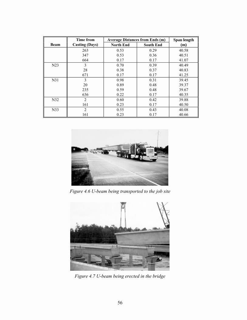
56
Average Distances from Ends (m)Beam
Time fromCasting (Days) North End South End
Span length(m)
263347664
0.530.530.17
0.290.360.17
40.5840.5141.07
N23 328
671
0.700.380.17
0.390.370.17
40.4940.8341.25
N31 320
235636
0.980.890.590.22
0.310.480.480.17
39.4539.3739.6740.35
N32 2161
0.600.23
0.420.17
39.8840.50
N33 2161
0.550.23
0.430.17
40.0840.66
Figure 4.6 U-beam being transported to the job site
Figure 4.7 U-beam being erected in the bridge
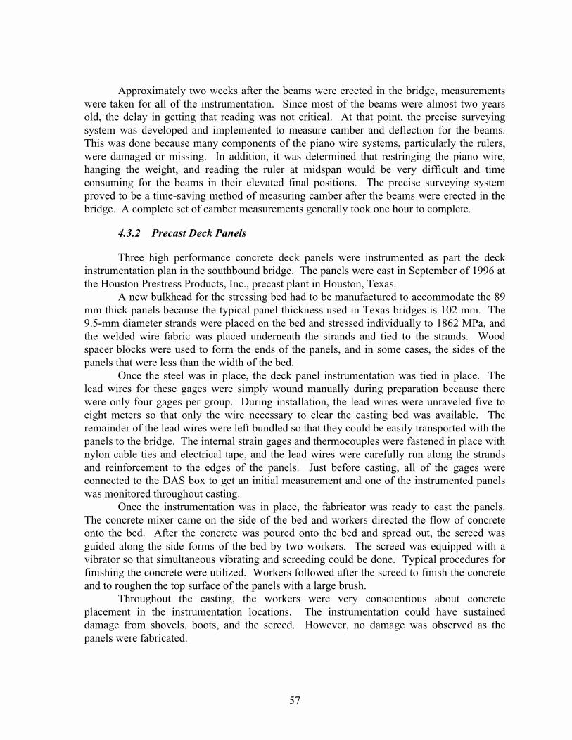
57
Approximately two weeks after the beams were erected in the bridge, measurementswere taken for all of the instrumentation. Since most of the beams were almost two yearsold, the delay in getting that reading was not critical. At that point, the precise surveyingsystem was developed and implemented to measure camber and deflection for the beams.This was done because many components of the piano wire systems, particularly the rulers,were damaged or missing. In addition, it was determined that restringing the piano wire,hanging the weight, and reading the ruler at midspan would be very difficult and timeconsuming for the beams in their elevated final positions. The precise surveying systemproved to be a time-saving method of measuring camber after the beams were erected in thebridge. A complete set of camber measurements generally took one hour to complete.
4.3.2 Precast Deck Panels
Three high performance concrete deck panels were instrumented as part the deckinstrumentation plan in the southbound bridge. The panels were cast in September of 1996 atthe Houston Prestress Products, Inc., precast plant in Houston, Texas.
A new bulkhead for the stressing bed had to be manufactured to accommodate the 89mm thick panels because the typical panel thickness used in Texas bridges is 102 mm. The9.5-mm diameter strands were placed on the bed and stressed individually to 1862 MPa, andthe welded wire fabric was placed underneath the strands and tied to the strands. Woodspacer blocks were used to form the ends of the panels, and in some cases, the sides of thepanels that were less than the width of the bed.
Once the steel was in place, the deck panel instrumentation was tied in place. Thelead wires for these gages were simply wound manually during preparation because therewere only four gages per group. During installation, the lead wires were unraveled five toeight meters so that only the wire necessary to clear the casting bed was available. Theremainder of the lead wires were left bundled so that they could be easily transported with thepanels to the bridge. The internal strain gages and thermocouples were fastened in place withnylon cable ties and electrical tape, and the lead wires were carefully run along the strandsand reinforcement to the edges of the panels. Just before casting, all of the gages wereconnected to the DAS box to get an initial measurement and one of the instrumented panelswas monitored throughout casting.
Once the instrumentation was in place, the fabricator was ready to cast the panels.The concrete mixer came on the side of the bed and workers directed the flow of concreteonto the bed. After the concrete was poured onto the bed and spread out, the screed wasguided along the side forms of the bed by two workers. The screed was equipped with avibrator so that simultaneous vibrating and screeding could be done. Typical procedures forfinishing the concrete were utilized. Workers followed after the screed to finish the concreteand to roughen the top surface of the panels with a large brush.
Throughout the casting, the workers were very conscientious about concreteplacement in the instrumentation locations. The instrumentation could have sustaineddamage from shovels, boots, and the screed. However, no damage was observed as thepanels were fabricated.

58
After the casting was completed, a tarp was placed over the entire bed. This tarp wassupported by four strands tensioned above the bed to hold it above the panels. The panelswere cured under the tarps without steam. The DAS box was connected to one set of panelgages to get measurements through transfer of the prestressing force the following morning.
Once the design strength was reached, the panels were transported to the bridge onflatbed trucks. The panels for the southbound main lanes bridge were erected beginning onSeptember 24, 1996. The panels for spans one and two of the northbound main lanes bridgewere erected beginning on September 26, 1996. Panels for span three were erected onOctober 17, 1996. A set of instrumentation measurements was obtained to record the strainsand cambers in the beams just before placement of the panels. Before the panels were placedin the bridges, strips of fiberboard needed to be glued on the inside and outside edges of eachflange of each beam. The typical dimensions of the fiberboard were 25.4 mm wide by 12.7mm thick. A crane was used to lift the panels and place them on the beams. Figure 4.8shows the placement of a panel and the fiberboard glued on the beam.
Figure 4.8 Precast deck panel being placed in the bridge
Complete erection of the panels occurred over the course of approximately two tothree weeks. Measurements were taken when some of the beams had only a fraction of thepanels on them. Table 4.5 summarizes the loads on the beams when these measurementswere taken. Measurements corresponding to post-placement of the deck panels were takenjust before casting of the northbound CIP deck.
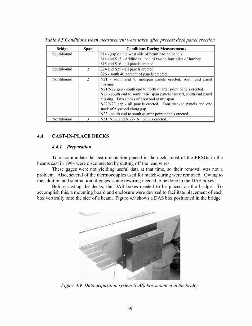
59
Table 4.5 Conditions when measurement were taken after precast deck panel erection
Bridge Span Conditions During MeasurementsSouthbound 1 S14 - gap on the west side of beam had no panels.
S14 and S15 - Additional load of two to four piles of lumber.S15 and S16 - all panels erected.
Southbound 2 S24 and S25 - all panels erected.S26 - south 40 percent of panels erected.
Northbound 2 N21 - south end to midspan panels erected, south end panelmissing.N21/N22 gap - south end to north quarter point panels erected.N22 - south end to south third span panels erected, south end panelmissing. Two stacks of plywood at midspan.N22/N23 gap - all panels erected. Four stacked panels and onestack of plywood along gap.N23 - south end to south quarter point panels erected.
Northbound 3 N31, N32, and N33 - All panels erected..
4.4 CAST-IN-PLACE DECKS
4.4.1 Preparation
To accommodate the instrumentation placed in the deck, most of the ERSGs in thebeams cast in 1994 were disconnected by cutting off the lead wires.
These gages were not yielding useful data at that time, so their removal was not aproblem. Also, several of the thermocouples used for match-curing were removed. Owing tothe addition and subtraction of gages, some rewiring needed to be done in the DAS boxes.
Before casting the decks, the DAS boxes needed to be placed on the bridge. Toaccomplish this, a mounting board and enclosure were devised to facilitate placement of eachbox vertically onto the side of a beam. Figure 4.9 shows a DAS box positioned in the bridge.
Figure 4.9 Data acquisition system (DAS) box mounted in the bridge

60
The construction of the mounting board and enclosure was done in the lab. The boardwas a 1220 mm wide by 1070 mm deep by 18.3 mm thick piece of plywood that was coveredwith a 3.2 mm thick piece of Plexiglas for protection. Large holes were cut in each end ofthe board to enable the gages to be hooked up to the box once the cover was on. A bracketwas made to account for the side slope of the beam and was placed on the bottom of theboard. The enclosure was constructed of 3.2 mm thick Plexiglas with 25.4 mm by 50.8 mmwood pieces used as framing. The enclosure was sealed with silicone and the entire assemblywas painted black.
At the site, anchor bolts were retrofitted into the beam, and the mounting board andbracket piece were placed onto the bolts and fastened mechanically. Next, the DAS box wasfixed onto the mounting board using steel brackets. Finally, the enclosure was fixed onto theboard over the DAS box using hinges and a latch. The boxes were positioned at the southeastquadrant of Beam N31 for the northbound main lanes bridge and at the southwest quadrant ofBeam S26 for the southbound main lanes bridge.
4.4.2 Instrumentation
Before the deck instrumentation could be installed, the longitudinal and transversereinforcement for the deck had to be completely tied into place by the workers. The VWgages and ERSGs were tied to the rebar using nylon cable ties. This proved to be aquestionable method of fixing the gages in place because the ties did not resist rotation of thegage around the rebar very well. Thermocouples were fixed into place with electrical tape.The lead wires were unspooled and tied along the top of the reinforcement and run to theends of the beams. Figure 4.10 shows a strain gage tied into the deck steel.
Figure 4.10 Instrumentation tied into cast-in-place deck reinforcement
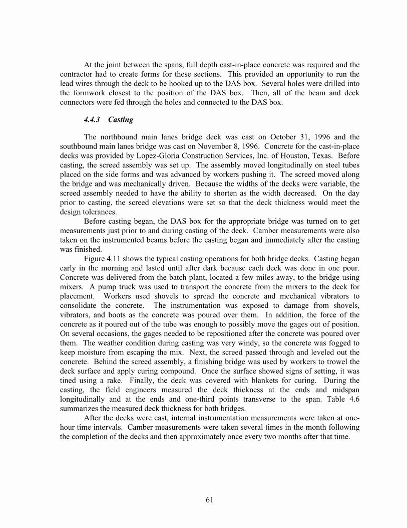
61
At the joint between the spans, full depth cast-in-place concrete was required and thecontractor had to create forms for these sections. This provided an opportunity to run thelead wires through the deck to be hooked up to the DAS box. Several holes were drilled intothe formwork closest to the position of the DAS box. Then, all of the beam and deckconnectors were fed through the holes and connected to the DAS box.
4.4.3 Casting
The northbound main lanes bridge deck was cast on October 31, 1996 and thesouthbound main lanes bridge was cast on November 8, 1996. Concrete for the cast-in-placedecks was provided by Lopez-Gloria Construction Services, Inc. of Houston, Texas. Beforecasting, the screed assembly was set up. The assembly moved longitudinally on steel tubesplaced on the side forms and was advanced by workers pushing it. The screed moved alongthe bridge and was mechanically driven. Because the widths of the decks were variable, thescreed assembly needed to have the ability to shorten as the width decreased. On the dayprior to casting, the screed elevations were set so that the deck thickness would meet thedesign tolerances.
Before casting began, the DAS box for the appropriate bridge was turned on to getmeasurements just prior to and during casting of the deck. Camber measurements were alsotaken on the instrumented beams before the casting began and immediately after the castingwas finished.
Figure 4.11 shows the typical casting operations for both bridge decks. Casting beganearly in the morning and lasted until after dark because each deck was done in one pour.Concrete was delivered from the batch plant, located a few miles away, to the bridge usingmixers. A pump truck was used to transport the concrete from the mixers to the deck forplacement. Workers used shovels to spread the concrete and mechanical vibrators toconsolidate the concrete. The instrumentation was exposed to damage from shovels,vibrators, and boots as the concrete was poured over them. In addition, the force of theconcrete as it poured out of the tube was enough to possibly move the gages out of position.On several occasions, the gages needed to be repositioned after the concrete was poured overthem. The weather condition during casting was very windy, so the concrete was fogged tokeep moisture from escaping the mix. Next, the screed passed through and leveled out theconcrete. Behind the screed assembly, a finishing bridge was used by workers to trowel thedeck surface and apply curing compound. Once the surface showed signs of setting, it wastined using a rake. Finally, the deck was covered with blankets for curing. During thecasting, the field engineers measured the deck thickness at the ends and midspanlongitudinally and at the ends and one-third points transverse to the span. Table 4.6summarizes the measured deck thickness for both bridges.
After the decks were cast, internal instrumentation measurements were taken at one-hour time intervals. Camber measurements were taken several times in the month followingthe completion of the decks and then approximately once every two months after that time.
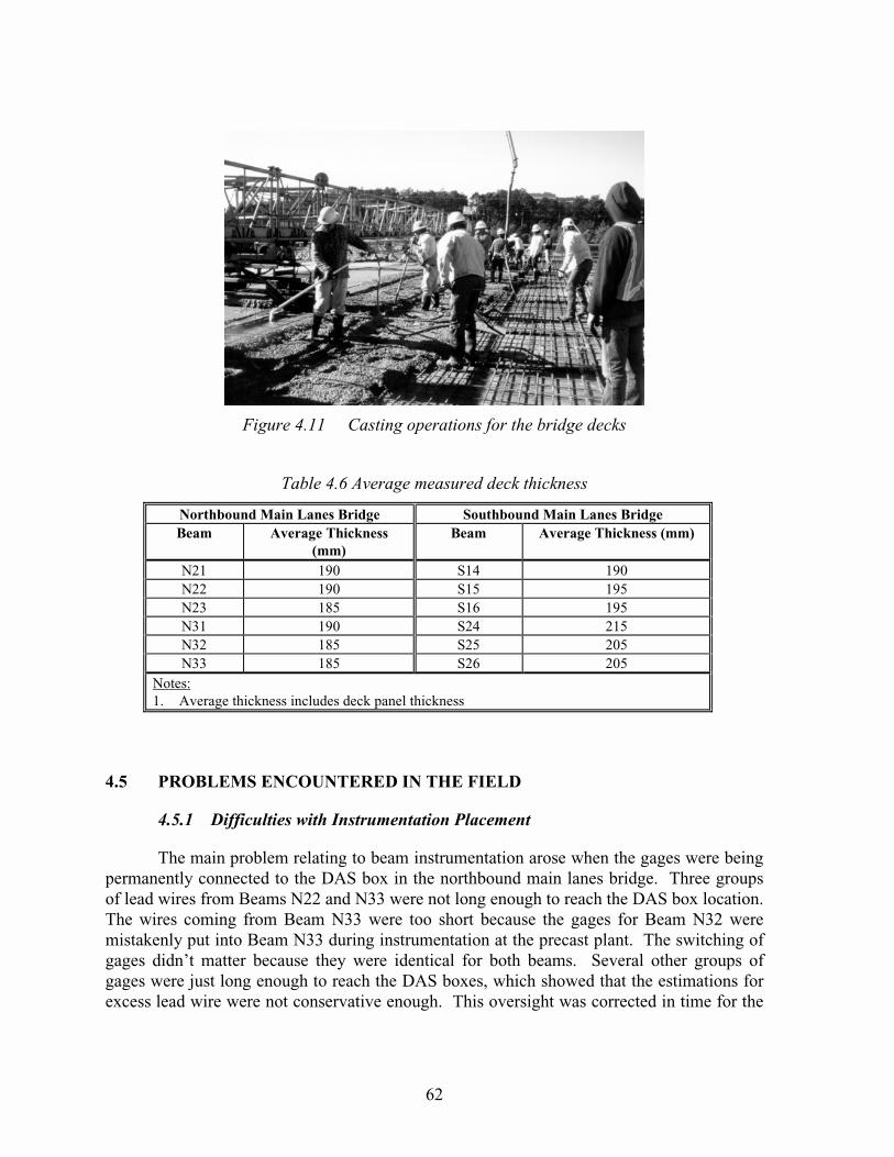
62
Figure 4.11 Casting operations for the bridge decks
Table 4.6 Average measured deck thickness
Northbound Main Lanes Bridge Southbound Main Lanes BridgeBeam Average Thickness
(mm)Beam Average Thickness (mm)
N21 190 S14 190N22 190 S15 195N23 185 S16 195N31 190 S24 215N32 185 S25 205N33 185 S26 205
Notes:1.� Average thickness includes deck panel thickness
4.5 PROBLEMS ENCOUNTERED IN THE FIELD
4.5.1 Difficulties with Instrumentation Placement
The main problem relating to beam instrumentation arose when the gages were beingpermanently connected to the DAS box in the northbound main lanes bridge. Three groupsof lead wires from Beams N22 and N33 were not long enough to reach the DAS box location.The wires coming from Beam N33 were too short because the gages for Beam N32 weremistakenly put into Beam N33 during instrumentation at the precast plant. The switching ofgages didn’t matter because they were identical for both beams. Several other groups ofgages were just long enough to reach the DAS boxes, which showed that the estimations forexcess lead wire were not conservative enough. This oversight was corrected in time for the
63
instrumentation of the beams in 1996. The wires coming from Beam N22 were too shortbecause the locations of the DAS boxes in the bridges were not finalized until after the beamswere erected. The solution to this problem was simply to make extension pieces of lead wireto allow those groups of gages to be connected to the DAS box.
Another problem occurred while installing the instrumentation in one of the precastdeck panels. In panel NS-32 that was placed between Beams S15 and S16 at midspan, thegages were positioned on the wrong side of the panel. These gages needed to be positionedoff a side of the panel that was parallel to the strands so that they would coincide with themidspan of Beam S15. Instead, the instrumentation was placed off a side of the panel thatwas transverse to the strands. The result was that the gages were out of alignment with therest of the deck and panel gages.
The remainder of the instrumentation problems occurred in the cast-in-place decks.In the deck for the northbound main lanes bridge, the exact vertical distances of the gagesabove the beams and panels were not measured. An assumption was made based upon thelocations of the reinforcement. This oversight was corrected while instrumenting the deckfor the southbound main lanes bridge. Another problem was that the nylon cable ties used totie the gages to the reinforcement didn’t fix the gages in place as well as desired. The gageshad a tendency to move if they were disturbed at all. Since the deck casting operation hadmany opportunities for disturbances, keeping the gages in their desired locations became aproblem. A more secure method for fixing the deck gages in place should have been used.
4.5.2 Damaged Instrumentation
Since most of the lead wires were embedded in the beams, the main opportunity fordamage was from the mechanical vibrator used to consolidate the concrete. However, a fewof the lead wires were damaged while the beams were being transported to the site anderected in the bridge. The exact cause of the damage was not determined, but one possibilitywas that the wires were inadvertently damaged by a heavy chain or a piece of equipment.These wires were spliced back together before being permanently connected to the DAS box.Subsequent measurements taken with the corresponding gages yielded good results.
The tensioned piano wire system was damaged in the field several times andultimately rendered unusable after the beams were transported to the site. During storage ofthe beams at the precast plant, C-clamps were routinely removed from the rulers leaving onlythe epoxy to hold the rulers in place. Since the five minute epoxy gel did not have long-termdurability, there was a chance that the ruler would fall off the aluminum plates. The rulerwas reattached to the plates using the impression of the plates on the old epoxy to repositionit. At other times, the rulers were missing and a new ruler had to be re-epoxied to thealuminum plates. Each camber measurement using a new ruler was adjusted based on theknown measurement on the other side of the beam. This adjustment assumed that both sidesof the beam experienced the same change in camber from the previous reading. Table 4.7describes which beams had rulers replaced while in storage and what adjustments were madeto subsequent camber measurements.

64
After the beams were transported to the job site, 17 of the 24 rulers were completelygone and many of the anchor bolts were sheared off. Since the camber system relied uponthe initial reading to be able to measure future cambers, it would have been very difficult tocorrelate new readings to the previous ones. The only way this could have been done was toassume an offset between the two sets of readings. Instead, the precise surveying system wasestablished at the job site.
Table 4.7 Adjustments to the tensioned piano wire camber and deflection system
Beam Side
Time from
Casting (Days) Operation
Adjustment To Future
MeasurementsN22 east 424 re-epoxied ruler noneS16 east 152 placed new ruler 6.86 mm lowerS16 west 424 re-epoxied ruler noneS25 west 287 placed new ruler 1.53 mm lowerS26 east 256 placed new ruler 4.83 mm lowerS26 east 321 placed new ruler 1.53 mm higher
The final incidence of damage to instrumentation occurred while the cast-in-placedecks were being poured. Several of the deck gages were stepped on and moved out ofposition during placement of the concrete. It would have been very difficult to avoid allpossible damage to the gages, considering the deck pouring procedures. However, a bettersystem of tying gages to the reinforcement would have reduced the magnitude of the damage.
4.5.3 Measurements
There were very few problems while taking measurements of the internal strain gagesand thermocouples with the DAS boxes. The post-transfer measurement for Beam N33 wasnot obtained because the DAS box was not turned on after the gage connectors were hookedup. However, this was not discovered until several days after the measurement and there wasno way to correct the problem. Since twelve beams were instrumented, this mistake was notcritical to the study. Also, the initial reading for Beam N23 was not taken prior to transfer.Since the baseline measurement was not obtained, the data from the strain gages was useless.However, the loss of that data was not critical because Beam N23 only had two ERSGs atmidspan.
Strain gage measurements were taken before the deck panels were placed on thebeams, but most of these measurements did not yield valid strains. The cause for thisproblem was probably due to an error with the DAS box or because of bad connections whenthe gage connectors were hooked up to the box. Since the beams were quite old, the previousmeasurements were used to represent the strain just before placement of the panels. Inaddition, the data gathered just before casting of the northbound bridge deck was not found
65
on the data storage module. Fortunately, several of the strain gages were working after thedecks were cast.
Measurement of camber seemed to present the greatest variety of problems. Both ofthe camber measuring systems were very sensitive to gusts of wind. For the tensioned pianowire system, wind caused the wire to vibrate causing the reading on the ruler to vary by asmuch as 3 mm. It was usually possible to get the wire to remain still long enough so that aprecise reading could be obtained. For the precise surveying system, wind caused the rod tomove, which made reading the rulers through the level very difficult.
Another problem with the tensioned piano wire system was that the lower bolt thatsupported the ruler began to interfere with the piano wire on Beam N23. Fortunately, thisproblem did not occur until the beam was 335 days old. In addition, the piano wiresfrequently broke, which meant that a lot of time was spent restringing the piano wire.
When the beams were ready for shipment to the job site, a communication breakdownbetween the researchers and the contractor resulted in some of the instrumented beams beingloaded onto the trucks before a final storage reading could be taken. Camber measurementswere obtained for all but one of the beams before shipment to the job site. This was not asignificant problem since the beams were very old at that time.
While taking camber measurements just before casting the southbound main lanesbridge deck, part of the screed assembly was being supported by the instrumented beams inspan one. This happened because of the skew of the bridge and because the casting began inspan one. While taking camber measurements after the deck panels were in the bridge,additional loads were introduced due to stacks of lumber and various pieces of equipmentused to construct the side forms for the deck. Also, some of the panels were not in placewhen camber and other measurements were taken because they hadn’t been shipped to thesite. Most of these problems were caused by the nature of construction and could not becontrolled. Camber measurements were taken just before the decks were cast to be used indetermining the deflection caused by the deck panels.

66
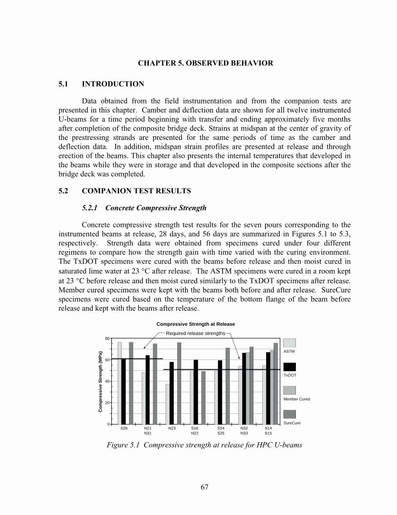
67
CHAPTER 5. OBSERVED BEHAVIOR
5.1 INTRODUCTION
Data obtained from the field instrumentation and from the companion tests arepresented in this chapter. Camber and deflection data are shown for all twelve instrumentedU-beams for a time period beginning with transfer and ending approximately five monthsafter completion of the composite bridge deck. Strains at midspan at the center of gravity ofthe prestressing strands are presented for the same periods of time as the camber anddeflection data. In addition, midspan strain profiles are presented at release and througherection of the beams. This chapter also presents the internal temperatures that developed inthe beams while they were in storage and that developed in the composite sections after thebridge deck was completed.
5.2 COMPANION TEST RESULTS
5.2.1 Concrete Compressive Strength
Concrete compressive strength test results for the seven pours corresponding to theinstrumented beams at release, 28 days, and 56 days are summarized in Figures 5.1 to 5.3,respectively. Strength data were obtained from specimens cured under four differentregimens to compare how the strength gain with time varied with the curing environment.The TxDOT specimens were cured with the beams before release and then moist cured insaturated lime water at 23 �C after release. The ASTM specimens were cured in a room keptat 23 �C before release and then moist cured similarly to the TxDOT specimens after release.Member cured specimens were kept with the beams both before and after release. SureCurespecimens were cured based on the temperature of the bottom flange of the beam beforerelease and kept with the beams after release.
Required release strengths
0
20
40
60
80
S26N31
N23 S16N22
S24S25
N32N33
S14S15
Co
mp
ress
ive
Str
eng
th (
MP
a)
N21
Compressive Strength at Release
ASTM
TxDOT
Member Cured
SureCure
Figure 5.1 Compressive strength at release for HPC U-beams
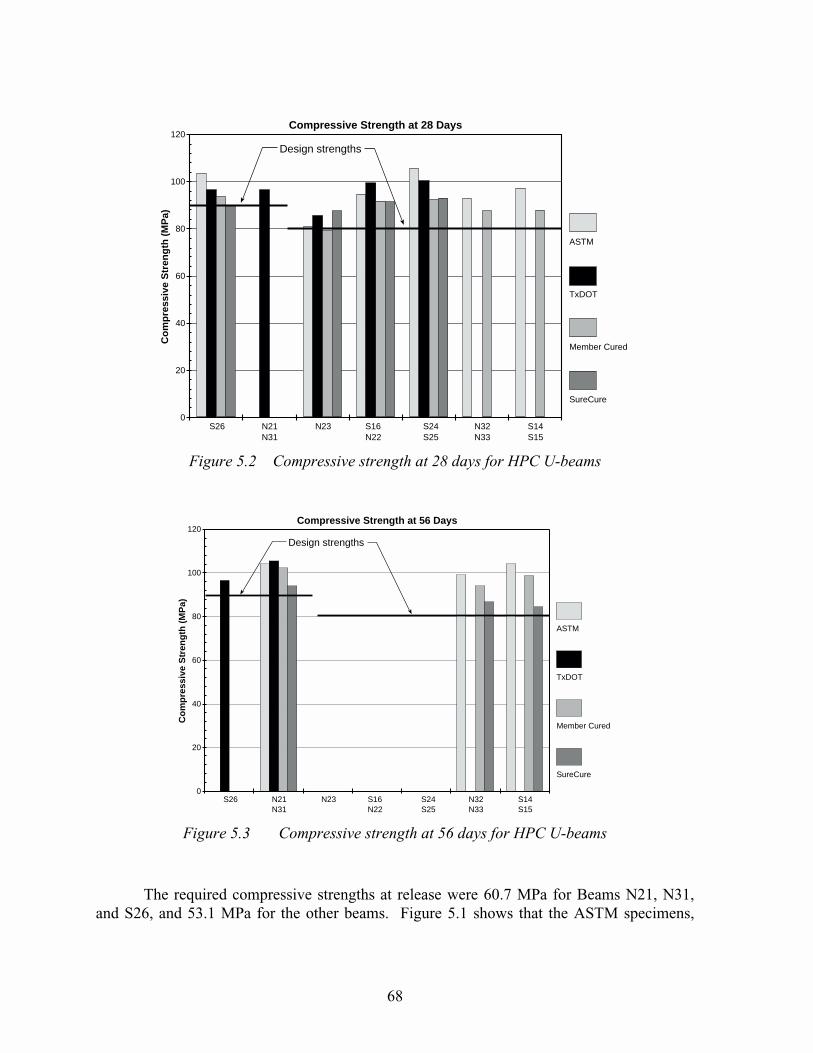
68
Design strengths
0
20
40
60
80
100
120
S26N31
N23 S16N22
S24S25
N32N33
S14S15
Co
mp
ress
ive
Str
eng
th (
MP
a)
N21
Compressive Strength at 28 Days
ASTM
TxDOT
Member Cured
SureCure
Figure 5.2 Compressive strength at 28 days for HPC U-beams
ASTM
TxDOT
Member Cured
SureCure
Design strengths
0
20
40
60
80
100
120
S26N31
N23 S16N22
S24S25
N32N33
S14S15
Co
mp
ress
ive
Str
eng
th (
MP
a)
N21
Compressive Strength at 56 Days
Figure 5.3 Compressive strength at 56 days for HPC U-beams
The required compressive strengths at release were 60.7 MPa for Beams N21, N31,and S26, and 53.1 MPa for the other beams. Figure 5.1 shows that the ASTM specimens,

69
with the exception of Beam S26, failed to reach the required release strength in four of theseven pours. Beam S26 was higher for all curing regimens because transfer of theprestressing force was at 7 days after casting. The SureCure specimens exhibited higherstrength than the other curing regimens in all but one of the pours. For that pour, theSureCure system was not working properly. The higher early strength of the SureCurespecimens can be attributed to the higher curing temperatures that the specimens experiencedwhile being match cured with the temperature of the bottom flange of the beam.
The 56-day design compressive strengths were 90.3 MPa for Beams N21, N31, andS26, and 80.0 MPa for the other beams. The compressive strengths at 28 and 56 days areshown in Figures 5.2 and 5.3, respectively. For some of the beams, the required strength hadalready been reached at 28 days and thus the 56 day strength was not measured. Thesefigures show the data that was available. At the ages of 28 and 56 days, the ASTMspecimens that were cured at lower temperatures showed higher strengths than the SureCurespecimens that were cured at higher initial temperatures. Furthermore, the SureCure andmember cured specimens that were stored near the beams in an uncontrolled environmentshowed lower strengths than the ASTM and TxDOT specimens that were kept in a controlledenvironment. The average strengths at release, 28 days, and 56 days for each curing regimeare summarized in Table 5.1.
Table 5.1 Average compressive strengths of HPC beam specimens under various curingregimens
Average Compressive Strength (MPa)Curing Regimen Release 28 days 56 daysASTM 53.2 95.7 102.6TxDOT 62.4 95.7 100.9Member Cured 68.0 88.7 98.3SureCure 70.9 90.6 88.4
Table 5.2 Average elastic moduli of HPC beam specimens
Average Elastic Modulus (GPa)1
Pour Beam(s) Release2 28 days3 56 days3
1 N23 44.3 43.94 N/A2 S16, N22 35.2 47.8 N/A3 S26 44.0 51.7 N/A5 N21, N31 40.0 N/A 46.37 S24, S25 37.8 44.5 N/A8 N32, N33 43.4 45.1 46.69 S14, S15 41.5 42.94 46.1
Notes:1.� Minimum specified elastic modulus was 41.4 GPa.2.� Data from tests of SureCure specimens.3.� Data from tests on member cured specimens.4.� Data from tests on ASTM cured specimens

70
To get the best representation of the compressive strength and deformation propertiesof the concrete at a specific age, the environment to which the concrete was subjected mustbe considered when choosing the appropriate curing regime. Before release, the SureCurespecimens provided the best representation of the beam concrete because the specimens werebeing cured at the same temperatures as the beams. After release, the member curedspecimens gave the best representation of the beam concrete because the specimens weresubjected to the same uncontrolled environment that the beams experienced.
An age-strength gain equation (Eq. 5.1) for the HPC beam mix was developed usingthe member cured specimens at all ages and the TxDOT cured specimens at release. A linearregression analysis was used to obtain a best fit curve for this data (correlation factor = 0.95).The data and the best fit curve are shown in Figure 5.4. Equation 5.1 was used in Chapter 6with an analytical time-step method for predicting prestress losses, camber, and deflection inthe instrumented beams.
� � � �� ��
����� �����
�
���
������� ����� �����
120
100
80
60
40
20
0
Co
mp
ress
ive
Str
eng
th (
MP
a)
Member cured specimens
TxDOT specimens
Proposed equation for strength gain
Equation 5.1
Age-Strength Gain for High Performance Concrete
Time after Casting (days)
0 14 28 42 56 70 84 98 112
Figure 5.4 Age-strength gain for HPC beam mix based on member cured specimens
5.2.2 Elastic Modulus of Concrete
The average elastic moduli of the beam concrete for all of the pours corresponding toinstrumented beams are summarized in Table 5.2. A minimum elastic modulus of 41.4 GPa
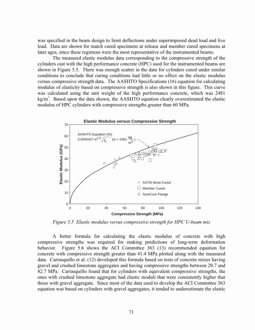
71
was specified in the beam design to limit deflections under superimposed dead load and liveload. Data are shown for match cured specimens at release and member cured specimens atlater ages, since these regimens were the most representative of the instrumented beams.
The measured elastic modulus data corresponding to the compressive strength of thecylinders cast with the high performance concrete (HPC) used for the instrumented beams areshown in Figure 5.5. There was enough scatter in the data for cylinders cured under similarconditions to conclude that curing conditions had little or no effect on the elastic modulusversus compressive strength data. The AASHTO Specifications (16) equation for calculatingmodulus of elasticity based on compressive strength is also shown in this figure. This curvewas calculated using the unit weight of the high performance concrete, which was 2481kg/m3. Based upon the data shown, the AASHTO equation clearly overestimated the elasticmodulus of HPC cylinders with compressive strengths greater than 60 MPa.
70
60
50
40
30
20
10
0
Ela
stic
Mo
du
lus
(GP
a)
ASTM Moist Cured
Member Cured
SureCure Flange
Elastic Modulus versus Compressive Strength
Compressive Strength (MPa)
0 20 40 60 80 100 120 140
AASHTO Equation (SI):
0.0000427 w1.5 (w = 2481 )f 'c
kg
m3
Figure 5.5 Elastic modulus versus compressive strength for HPC U-beam mix
A better formula for calculating the elastic modulus of concrete with highcompressive strengths was required for making predictions of long-term deformationbehavior. Figure 5.6 shows the ACI Committee 363 (13) recommended equation forconcrete with compressive strength greater than 41.4 MPa plotted along with the measureddata. Carrasquillo et al. (12) developed this formula based on tests of concrete mixes havinggravel and crushed limestone aggregates and having compressive strengths between 20.7 and82.7 MPa. Carrasquillo found that for cylinders with equivalent compressive strengths, theones with crushed limestone aggregate had elastic moduli that were consistently higher thatthose with gravel aggregate. Since most of the data used to develop the ACI Committee 363equation was based on cylinders with gravel aggregates, it tended to underestimate the elastic

72
moduli for the beams in this study, which were cast from a concrete mix having crushedlimestone aggregate.
( ) ( )
( ) ( )
70
60
50
40
30
20
10
0
Ela
stic
Mo
du
lus
(GP
a)
ASTM Moist Cured
Member Cured
SureCure Flange
Elastic Modulus versus Compressive Strength
Compressive Strength (MPa)
0 20 40 60 80 100 120 140
AASHTO Equation (SI):
0.0000427 w1.5 (w = 2481 )f 'c
kg
m3
Proposed Equation (SI):
(3.10 + 11.29) 1.5 w = 2481f 'c
kg
m3w
2323
f 'c
kg
m3w
2323
ACI 363 Equation (SI):
(3.32 + 6.89) 1.5 w = 2481
Figure 5.6 Proposed equation for elastic modulus for HPC U-beams
A more accurate equation for calculating the elastic modulus (GPa) for the highperformance concrete used to cast the beams in this study was developed by adopting theform of the ACI Committee 363 equation and fitting a new curve to the measured data. Theproposed equation for elastic modulus is as follows:
� �� ��
���� ����� � � �
����
��� ����
��
� �
�
This equation is shown graphically in Figure 5.6 along with the AASHTO and theACI Committee 363 equations. The proposed equation is valid for the high performanceconcrete mix used for the beams in this study and for the range of compressive strengthsrepresented by the test data.
5.2.3 Creep and Shrinkage Properties of Concrete
As mentioned in Sec. 3.6.4, Farrington (8) tested eighteen creep specimens cast fromthe high performance concrete used to make the beams in this study. The effects of curingtemperature, age of loading, and level of loading were examined as part of that study. Thecreep data used in this study were taken from the specimens loaded at one day under all three
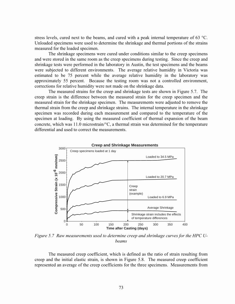
73
stress levels, cured next to the beams, and cured with a peak internal temperature of 63 �C.Unloaded specimens were used to determine the shrinkage and thermal portions of the strainsmeasured for the loaded specimen.
The shrinkage specimens were cured under conditions similar to the creep specimensand were stored in the same room as the creep specimens during testing. Since the creep andshrinkage tests were performed in the laboratory in Austin, the test specimens and the beamswere subjected to different environments. The average relative humidity in Victoria wasestimated to be 75 percent while the average relative humidity in the laboratory wasapproximately 55 percent. Because the testing room was not a controlled environment,corrections for relative humidity were not made on the shrinkage data.
The measured strains for the creep and shrinkage tests are shown in Figure 5.7. Thecreep strain is the difference between the measured strain for the creep specimen and themeasured strain for the shrinkage specimen. The measurements were adjusted to remove thethermal strain from the creep and shrinkage strains. The internal temperature in the shrinkagespecimen was recorded during each measurement and compared to the temperature of thespecimen at loading. By using the measured coefficient of thermal expansion of the beamconcrete, which was 11.0 microstrain/�C, a thermal strain was determined for the temperaturedifferential and used to correct the measurements.
3000
2500
2000
1500
1000
500
0
Co
mp
ress
ive
Str
ain
(x
10-6
mm
/mm
)
Creep and Shrinkage Measurements
Time after Casting (days)0 50 100 150 200 250 300 350 400
Creep specimens loaded at 1 day
Shrinkage strain includes the effectsof temperature differences
Loaded to 34.5 MPa
Creepstrain(example)
Loaded to 20.7 MPa
Loaded to 6.9 MPa
Average Shrinkage
Figure 5.7 Raw measurements used to determine creep and shrinkage curves for the HPC U-beams
The measured creep coefficient, which is defined as the ratio of strain resulting fromcreep and the initial elastic strain, is shown in Figure 5.8. The measured creep coefficientrepresented an average of the creep coefficients for the three specimens. Measurements from

74
all three specimens could be used because the level of loading did not to influence theultimate creep coefficient (8). Averaging the creep coefficients for the three specimensallowed more data to be used for determining a best fit creep equation.
3.0
2.5
2.0
1.5
1.0
0.5
0.0
Cre
ep C
oef
fici
ent
(Cct
)
Time after Loading (days)
0 50 100 150 200 250 300 350 400
Equation 5.3
ACI 209 Prediction
Equation 5.4Raw Data
Figure 5.8 ACI prediction and proposed equations for creep coefficient
Two best fit curves were developed for the measured creep data as shown in Figure5.8. The creep curves, given in Eqs. 5.3 and 5.4, were based on different time functions.These curves are based on data for 372 days of loading on the test specimens. Thecorrelation factors for these curves were very close (0.997 for Eq. 5.3 and 0.996 for Eq. 5.4),but the ultimate creep coefficients were quite different. The ultimate creep coefficients forthe HPC beam mix were 2.28 in Eq. 5.3 and 1.76 in Eq. 5.4. Equation 5.3 is used in Sec. 6.4for analytical predictions of prestress losses, camber, and deflection. Both of these equationsare used in Chapter 6 for developing camber and deflection multipliers.
� ���
� � ������
���
����
�
�
��
�
�� ���
� ���
� � ������
���
����
�
�
��
�
�����
The ACI Committee 209 prediction (19) of creep coefficient for this specimen was includedin Figure 5.8 as a comparison to the measured creep coefficient. A detailed description of theACI Committee 209 procedures for determining creep coefficient is presented in the report

75
by Farrington (8). The form of the ACI creep function is different than the forms of the bestfit curves. The ultimate creep coefficient for the ACI Committee 209 curve was 3.35. TheACI prediction of ultimate creep overestimated the measured ultimate creep coefficientsshown in Eqs. 5.3 and 5.4 by 47 and 90 percent, respectively.
The average measured shrinkage strain for the high-temperature cured specimens isshown in Figure 5.9. These measurements were sensitive to the relative humidity andambient temperature fluctuations in the uncontrolled environment in the room where the testswere performed. Increases in the relative humidity would cause moisture in the air to beabsorbed by the concrete resulting in swelling of the concrete. This caused the measuredshrinkage strain to be distorted.
700
600
500
400
300
200
100
0
Sh
rin
kag
e S
trai
n (
x 10
-6m
m/m
m)
Time after Casting (days)
0 50 100 150 200 250 300 350 400
Measured data(temp. corrected)
ACI 209 Prediction
Equation 5.5
Figure 5.9 ACI prediction and proposed equation for shrinkage strain
The ACI Committee 209 prediction (19) of shrinkage for these specimens is includedin Figure 5.9 as a comparison to the measured data. Equation 5.5 represents the best fit curvethrough the data shown in Figure 5.9. However, the measured data needed to be corrected forthe shrinkage strain that occurred between stripping of the cylinders and the baseline Demecreadings. The amount of time that occurred between those two events was approximately 12hours. An approximation of the additional shrinkage strain was made by shifting the best fitcurve (Eq. 5.5) up by 12 hours and then determining a correction based upon the slope of thebest fit curve at that point. A new best fit curve, given in Eq. 5.6, was developed after thiscorrection in which the ultimate shrinkage strain was 456 microstrain.

76
� � � �� �� �
���
���
�
� � ������
�
�
��
�
��������
� � � �� �� �
���
���
�
� � ������
�
�
��
�
��������
The ACI prediction of ultimate shrinkage, which was 738 microstrain, overestimatedthe measured ultimate shrinkage of the high performance concrete by 62 percent. Equation5.6 was developed to provide an accurate means of predicting the long-term shrinkage of thebeams cast with this HPC mix. This equation is used in Chapter 6 for analytical predictionsof prestress losses.
5.3 FIELD MEASUREMENTS
5.3.1 Camber and Deflection
The measured time-dependent camber and deflection responses at midspan of thetwelve instrumented U-beams are shown in Figures 5.10 to 5.21. The camber and deflectionresponse history for each beam was monitored from the time just before transfer to the timefive months after the cast-in-place decks were completed. Significant events are noted alongthe time axis of Figures 5.10 to 5.21, reflecting the important stages of construction of thecomposite prestressed concrete bridge.
180
160
140
120
100
80
60
40
20
0
Mid
span
Cam
ber
(m
m)
Time after Casting (days)
0 100 200 300 400 500 600 700 800 900 1000
A placement in bridge
B partial panel erection
C complete panel erection
D casting of deck slab
Ls span length
Raw measurementsAnalytically corrected measurementsMeasurements not adjusted for thermal movementsAssumed camber based on readings at 713 and 734 days
In storage
A BCD
Ls = 40.65 mLs = 40.45 m Ls = 40.90 m
Time- Dependent CamberBeam N21
Figure 5.10 Measured midspan camber and deflection response for Beam N21

77
140
120
100
80
60
40
20
0
-20
Mid
span
Cam
ber
(m
m)
Time after Casting (days)
0 100 200 300 400 500 600 700 800 900 1000
A placement in bridge
B partial panel erection
C complete panel erection
D casting of deck slab
Ls span length
Raw measurementsMeasurements adjusted for span length onlyMeasurements adjusted for thermal gradients and span lengthAssumed cambers based on readings at 741 and 762 days
In storage
A BC
DLs = 40.60 m
Ls = 40.58 mLs = 41.07 m
Time-Dependent CamberBeam N22
Ls = 40.46 m Ls = 40.51 m
Figure 5.11 Measured midspan camber and deflection response for Beam N22
140
120
100
80
60
40
20
0
-20
Mid
span
Cam
ber
(m
m)
Time after Casting (days)
0 100 200 300 400 500 600 700 800 900 1000
A placement in bridge
B partial panel erection
C complete panel erection
D casting of deck slab
Ls span length
Raw measurementsMeasurements adjusted for span length onlyAssumed cambers based on readings at 748 and 769 days
In storage
A BC
D
Ls = 40.49 m
Ls = 41.25 m
Time-Dependent CamberBeam N23
Ls = 40.83 m
Figure 5.12 Measured midspan camber and deflection response for Beam N23
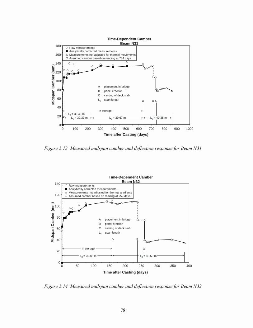
78
180
160
140
120
100
80
60
40
20
0
Mid
span
Cam
ber
(m
m)
Time after Casting (days)
0 100 200 300 400 500 600 700 800 900 1000
Raw measurementsAnalytically corrected measurementsMeasurements not adjusted for thermal movementsAssumed camber based on reading at 734 days
In storage
A B C
Ls = 39.45 mLs = 39.67 m Ls = 40.35 m
Time-Dependent CamberBeam N31
Ls = 39.37 m
A placement in bridge
B panel erection
C casting of deck slab
Ls span length
Figure 5.13 Measured midspan camber and deflection response for Beam N31
140
120
100
80
60
40
20
0
Mid
span
Cam
ber
(m
m)
Time after Casting (days)
0 50 100 150 200 250 300 350 400
A placement in bridge
B panel erection
C casting of deck slab
Ls span length
Raw measurementsAnalytically corrected measurementsMeasurements not adjusted for thermal gradientsAssumed camber based on reading at 259 days
In storage
A B
C
Ls = 40.50 m
Time-Dependent CamberBeam N32
Ls = 39.88 m
Figure 5.14 Measured midspan camber and deflection response for Beam N32

79
140
120
100
80
60
40
20
0
Mid
span
Cam
ber
(m
m)
Time after Casting (days)
0 50 100 150 200 250 300 350 400
A placement in bridge
B panel erection
C casting of deck slab
Ls span length
Raw measurementsAnalytically corrected measurementsMeasurements not adjusted for thermal movementsAssumed camber based on reading at 259 days
In storage
A B
C
Ls = 40.66 m
Time-Dependent CamberBeam N33
Ls = 40.08 m
Figure 5.15 Measured midspan camber and deflection response for Beam N33
140
120
100
80
60
40
20
0
Mid
span
Cam
ber
(m
m)
Time after Casting (days)
0 50 100 150 200 250 300 350 400
Raw measurementsAnalytically corrected measurementsMeasurements not adjusted for thermal movementsAssumed camber based on readings at 227 and 256 days
In storage
A B
D
Ls = 35.55 m
Time-Dependent CamberBeam S14
Ls = 34.67 m
A placement in bridge
B partial panel erection
C complete panel erection
D casting of deck slab
Ls span lengthC
Figure 5.16 Measured midspan camber and deflection response for Beam S14

80
140
120
100
80
60
40
20
0
Mid
span
Cam
ber
(m
m)
Time after Casting (days)
0 50 100 150 200 250 300 350 400
Raw measurementsAnalytically corrected measurementsMeasurements not adjusted for thermal movementsAssumed camber based on reading at 227 days
In storage
A B
Ls = 36.01 m
Time-Dependent CamberBeam S15
Ls = 35.18 m
A placement in bridge
B panel erection
C casting of deck slab
Ls span length
C
Figure 5.17 Measured midspan camber and deflection response for Beam S15
140
120
100
80
60
40
20
0
Mid
span
Cam
ber
(m
m)
Time after Casting (days)
0 100 200 300 400 500 600 700 800 900 1000 1100
Raw measurementsAnalytically corrected measurementsMeasurements not adjusted for thermal movementsAssumed camber based on reading at 770 days
In storage
A B
Ls = 36.89 m
Time-Dependent CamberBeam S16
Ls = 35.54 m
A placement in bridge
B panel erection
C casting of deck slab
Ls span length C
Ls = 35.93 m
Figure 5.18 Measured midspan camber and deflection response for Beam S16

81
120
100
80
60
40
20
0
-20
-40
Mid
span
Cam
ber
(m
m)
Time after Casting (days)
0 100 200 300 400 500 600 700 800 900 1000
Rawmeasurements
Analyticallycorrectedmeasurements
Measurementsnot adjusted forthermal movements
Assumed camberbased on readingat 729 days
In storage
A B
Ls = 39.83 m
Time-Dependent CamberBeam S24
Ls = 39.45 m
A placement in bridge
B panel erection
C casting of deck slab
Ls span length
C
Ls = 39.33 m
Figure 5.19 Measured midspan camber and deflection response for Beam S24
120
100
80
60
40
20
0
-20
-40
Mid
span
Cam
ber
(m
m)
Time after Casting (days)
0 100 200 300 400 500 600 700 800 900 1000
Rawmeasurements
Analyticallycorrectedmeasurements
Measurementsnot adjusted forthermal movements
Assumed camberbased on readingat 729 days
In storage
A B
Ls = 40.33 m
Time-Dependent CamberBeam S25
A placement in bridge
B panel erection
C casting of deck slab
Ls span length
C
Ls = 39.85 mLs = 39.91 m
Figure 5.20 Measured midspan camber and deflection response for Beam S25

82
180
160
140
120
100
80
60
40
20
0
Mid
span
Cam
ber
(m
m)
Time after Casting (days)
0 100 200 300 400 500 600 700 800 900 1000
Raw measurementsMeasurements adjusted for span length onlyAssumed camber based on readings at 734 and 763 days
In storage
A B
Ls = 40.84 m
Time-Dependent CamberBeam S26
A placement in bridge
B partial panel erection
C complete panel erection
D casting of deck slab
Ls span length C
Ls = 40.29 m
Ls = 40.43 m
D
Figure 5.21 Measured midspan camber and deflection response for Beam S26
Raw midspan camber measurements are shown in each figure to represent the beamcamber under the conditions at the time of the measurement. This means that large thermalgradients could have been present at the time of the reading and the bearing locations couldhave been different from the design bearing locations for that beam in the completed bridge.For all of the beams, the span length during storage was smaller than the design span lengthin the bridge. The measured span lengths during storage and their applicable time periods areshown at the bottom of each figure. In addition, most of the camber readings were taken inthe afternoon when large thermal gradients were present in the beams. As a result of all ofthese varying span and temperature conditions, the raw camber measurements tended to beerratic.
The analytically corrected camber measurements are of more interest for identifyingthe shape of the camber response over time and for making comparisons of camber growthfor similar beams. The analytical correction for span length was a correction on the self-weight deflection of the beam. It adjusted the measured camber to the value it would havebeen if the beam’s bearing locations were the same as in the bridge. After the beams wereerected in the bridge, this correction was no longer necessary. Using the second area-moment theorem for determining relative deflections, Eqs. 5.7 and 5.8 were derived tocalculate the dead load deflections at midspan under the actual support conditions and underthe bridge support conditions, respectively. Note that in Eq. 5.8, the portions of the beamthat cantilevered past the bearings were considered negligible. Equation 5.9 represents thecorrection to the camber measurement. Also note that Eqs. 5.1 and 5.2 were used fordetermining the compressive strength and modulus of elasticity at the time of the change insupport conditions in storage the elastic modulus. At late ages, the small changes in modulus

83
of elasticity did not affect the magnitude of the beam self-weight correction. The magnitudeof this correction ranged from two to five millimeters.
������ ��
��
� ��
��
� ��
���
�!
�
���" " " " " " " " ������ � � � ��
����
�
��
�
��
�
�
�
�
#�$%� #���"
����! ������
& ��'� & (� ������ #�$%� ) ������
wherew = distributed weight of the beam (N/m)E = elastic modulus of concrete as determined by Eq. 5.2 (GPa)I = moment of inertia of beam (m4)Ls= measured span length in storage (m)Lo = average measured overhang from the center line of bearing (m)Lb = design span length in the bridge (m)storage = deflection resulting from beam weight under storage support conditionsbridge = deflection resulting from beam weight under bridge support conditionsmeasurement = correction to measured camber for varying support conditions
In determining the analytical correction for camber resulting from a thermal gradientin a beam, the strain distribution resulting from changes in temperature with reference to auniform temperature profile of 20 �C was determined. The uniform temperature profilecorresponded to zero thermally induced movement of the beam at 20 �C. The straindistribution was usually nonlinear, corresponding to the nonlinear temperature gradientsobserved in the beams, which are shown in Sec. 5.3.5. No axial or bending stresses wereassumed to be induced in the beam since the support conditions were modeled as a pin and aroller for simple span supports. As a result, self-equilibrating stresses were assumed to bedeveloped in the beam from the strains induced in the member that countered the distortionof the section resulting from the nonlinear thermal strain profile (53). A constant curvaturealong the beam length was assumed based on the resultant strain profile and was used tocalculate a theoretical camber resulting from a temperature gradient.
Details about measured thermal movements can be found in Sec. 5.3.6. Equation5.10 represents the theoretical camber or deflection at midspan resulting from a thermalgradient. The theoretical camber resulting from thermal gradients was as large as 20millimeters for some of the beams during storage.
�� �&�* ���"
� �������
�
��
�
��
where�t = curvature caused by the internal self-equilibrating forcesLs = measured span length (m)

84
The plots shown in Figures 5.10 to 5.21 represent the time-dependent camberbehavior of the beams after all possible analytical corrections were applied to the raw cambermeasurements. As shown in those graphs, a majority of the camber growth for all of thebeams occurred in the first 80 to 100 days of storage. After that point, the camber responseflattened out.
For some of the measurements, a correction for thermal movements was not possiblebecause the internal temperatures in that beam or its companion beam were not taken at thattime. The measurements not corrected for thermal movements are shown as an open triangle,as can be seen in Figure 5.10. After the beams were erected in the bridge, corrections werenot made for thermal movements because many of the internal instrumentation readings werenot valid. In addition, the corrections became very sensitive to the deck temperatures whenthe sections became composite. Since nearly all of the camber readings after erection weretaken in the morning, the magnitudes of the thermal movements were probably small.
For Beams N22, N23, and S26, corrections for thermal movements were not possible.Figure 5.21 shows the time-dependent camber response for Beam S26. Since most of thereadings were in the afternoon, it was not possible to remove the thermal effects from thecamber plot. The measurements up to 150 days demonstrated the influence that thermalgradients had on the camber readings. The shape of the response curve shows the large early-age camber growth before the curve assumed the characteristic flattened shape where themeasurements were farther apart. The fluctuations in the response curve for Beam S26 weredue to uncorrected temperature gradient effects.
Figure 5.12 shows the time-dependent camber response for Beam N23. For thisbeam, several morning readings were taken which were used to eliminate the thermal effects.In contrast to the camber plot for Beam S26 shown in Figure 5.21, the response shown inFigure 5.12 was smoother in the first 150 days of measurements and the time-dependentcamber response was similar in shape to the beams whose measurements were corrected forthermal movements.
Figure 5.20 shows the time-dependent camber for Beam S25, which was cast onNovember 10, 1994. This beam represents the typical camber response for the group ofbeams that were stored at the prestressing plant for almost two years before being erected inthe bridge.
An initial camber of 49.4 mm was measured immediately after release at 1.15 dayswhile the beam was still on the prestressing bed. After determining a thermal correction, theadjusted camber was 44.1 mm. For this measurement, the span length (Ls) wasapproximately 40.20 meters, which was 0.46 meters less than the length of the beam. Thesupport conditions on the prestressing bed were similar for all of the instrumented beams andwere quite close to the support conditions in the bridge.
After release, the beam was moved into storage and supported with wooden blockspositioned in from the ends of the beam. The measured camber increased to 53.5 mm due toshortening of the span length. After applying the analytical corrections for supportconditions and thermal movements, the camber became 45.2 mm, which was reasonablyclose to the camber immediately after release. The measured span length during storage was

85
39.85 meters, as shown above the time axis in Figure 5.20. The final span length shown wasthe design span length in the bridge to which all of the camber measurements were adjusted.
During the first 80 days in storage, the beam camber grew to 75.2 mm. Beam S25was kept in storage for 620 days and was moved one time during storage. As shown inFigure 5.20, the camber grew to 86.1 mm during that period of time.
At 620 days, the beam was transported to Houston and placed in the bridge. This isshown in Figure 5.20 as event A in the response history of the beam. At that time, camberwas no longer measured using the piano wire system and the precise surveying system wasimplemented. For most of the beams, the surveyed camber agreed closely with the last pianowire camber measurement. However, Beams N31, S16, S24, and S26 displayed positive ornegative differentials of approximately four to six millimeters. The reason for this relativelysmall differential was probably due to error in determining the exact bearing elevations.Another possible source of error was in the thickness of the plywood pads that were placedunder the beams before transfer. The pad thickness was needed to adjust the baseline pianowire readings for some of the beams. Variation in the actual pad thickness would shift thecamber response curve up or down slightly relative to the surveyed cambers.
At 676 days, the placement of the precast deck panels began. This is shown as eventB in Figure 5.20. The measured camber at 676 days was 85.9 mm. The measured camber at700 days of 58.2 mm was assumed to be a reasonable approximation to the camber afterplacement of the panels. The elastic deflection resulting from the weight of the panels wasapproximately 27.7 mm.
The cast-in-place deck for the southbound bridge was poured 729 days after BeamS25 was cast. This is shown as event C in Figure 5.20. The measured camber before castingthe deck was 47.8 mm. Immediately after the deck was poured, the measured camber was7.1 mm. The elastic deflection resulting from the weight of the deck slab was 40.7 mm.Camber measurements were taken as late as 848 days after casting, where the camber haddecreased slightly to 2.5 mm. At that time, guardrails had not been placed on the bridge.
The time-dependent camber responses for the other beams were similar to that ofBeam S25. The main difference was that the group of beams cast in February of 1996 werestored at the prestressing plant 460 to 520 days less than the other beams.
Measurements for the elastic deflection resulting from the superimposed loading ofthe deck panels were not obtained immediately after placement because, for most of thebeams, only a fraction of the panels were erected at the times of measurement. All of thecamber response diagrams show a dashed line and symbols representing the assumedinstantaneous response of the beams based upon measurements taken within several days ofthe measurements before the panels were erected. Section 4.3.2 summarizes the conditionsduring the panel measurements.
The camber responses shown in Figures 5.10 to 5.12, 5.16, and 5.21 have anintermediate stage where only part of the panels were erected on each beam during themeasurement. The elastic deflection resulting from the panels for these beams was assumedto be the sum of the deflections from the two stages of panel placement. This assumptionwas made knowing that the camber probably changed a very small amount owing to the
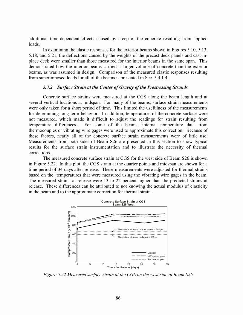
86
additional time-dependent effects caused by creep of the concrete resulting from appliedloads.
In examining the elastic responses for the exterior beams shown in Figures 5.10, 5.13,5.18, and 5.21, the deflections caused by the weights of the precast deck panels and cast-in-place deck were smaller than those measured for the interior beams in the same span. Thisdemonstrated how the interior beams carried a larger volume of concrete than the exteriorbeams, as was assumed in design. Comparison of the measured elastic responses resultingfrom superimposed loads for all of the beams is presented in Sec. 5.4.1.4.
5.3.2 Surface Strain at the Center of Gravity of the Prestressing Strands
Concrete surface strains were measured at the CGS along the beam length and atseveral vertical locations at midspan. For many of the beams, surface strain measurementswere only taken for a short period of time. This limited the usefulness of the measurementsfor determining long-term behavior. In addition, temperatures of the concrete surface werenot measured, which made it difficult to adjust the readings for strain resulting fromtemperature differences. For some of the beams, internal temperature data fromthermocouples or vibrating wire gages were used to approximate this correction. Because ofthese factors, nearly all of the concrete surface strain measurements were of little use.Measurements from both sides of Beam S26 are presented in this section to show typicalresults for the surface strain instrumentation and to illustrate the necessity of thermalcorrections.
The measured concrete surface strain at CGS for the west side of Beam S26 is shownin Figure 5.22. In this plot, the CGS strain at the quarter points and midspan are shown for atime period of 34 days after release. These measurements were adjusted for thermal strainsbased on the temperatures that were measured using the vibrating wire gages in the beam.The measured strains at release were 13 to 22 percent higher than the predicted strains atrelease. These differences can be attributed to not knowing the actual modulus of elasticityin the beam and to the approximate correction for thermal strain.
1200
1000
800
600
400
200
0
Co
mp
ress
ive
Str
ain
(x
10-6
mm
/mm
)
Concrete Surface Strain at CGSBeam S26 West
Time after Release (days)0 5 10 15 20 25 30 35
Theoretical strain at quarter points = 661 µε
MidspanNW quarter pointSW quarter point
Theoretical strain at midspan = 605 µε
Figure 5.22 Measured surface strain at the CGS on the west side of Beam S26

87
As expected, the strains at midspan remained less than the strains at the quarter pointsowing to the larger dead load moment at midspan. The measured surface strains for thisbeam over 34 days were in close agreement with the measured internal strains for Beam S26that are shown in Figure 5.27. The measured strains from the two sources are within 6percent of each other at release and are within 4 percent of each other at 34 days.Unfortunately, surface strain readings for this beam were not taken past 34 days, which wastypical for all of the beams.
Figure 5.23 illustrates the importance of correct temperature data for the concretesurface strain measurements. In this plot, the CGS strains at the quarter points and midspanof the east side of Beam S26 are shown. These measurements were adjusted for temperaturedifferences using the internal temperatures from the vibrating wire gages on the west side ofthe beam. One problem with the data was that the measured strains at midspan were higherthan the strains at the southeast quarter point. Also, the measured strains at release for themidspan and southwest quarter point locations were approximately 44 percent higher than themeasured internal strains on the west side shown in Figure 5.27. At 34 days, the measuredstrains at release for the midspan and southwest quarter point locations were approximately31 percent higher than the strains shown in Figure 5.27. Obviously, the surface strainmeasurements for the east side of the beam should not be relied upon to represent the strainbehavior of Beam S26.
1600
1400
1200
1000
800
600
400
200
0
Co
mp
ress
ive
Str
ain
(x
10-6
mm
/mm
)
Concrete Surface Strain at CGSBeam S26 East
Time after Release (days)0 5 10 15 20 25 30 35
Theoretical strain at quarter points = 661 µε
MidspanNE quarter pointSE quarter point
Theoretical strain at midspan = 605 µε
Figure 5.23 Measured surface strain at the CGS on the east side of Beam S26

88
5.3.3 Internally Measured Strain at the Center of Gravity of the Prestressing Strands
Strain measurements from the embedded gages provided the most useful long-termstrain data. The data shown in this section focus on measured strain at the center of gravityof the prestressing strands (CGS). The measured strains at CGS were of interest fordetermining immediate and long-term prestress losses.
Both the electrical resistance strain gages (ERSG) and the vibrating wire (VW) gageswere thermally compensated so that the effect of differences in uniform temperature changesbetween readings was eliminated. Strain corrections were not made for changes in supportconditions, as was done for the camber measurements. Since the initial strain measurements,or baseline readings, were not taken until just before release, the effects of strand relaxation,shrinkage, and changes in temperature of the strand were not part of the strain measurements.The predicted strains at release included prestress losses of 2 percent for relaxation and 2percent for shrinkage and temperature effects in addition to the prestress loss resulting fromelastic shortening. Transformed section properties and the measured modulus of elasticity atrelease were used to compute the theoretical release strains.
The measured strains at the CGS at midspan for several beams are shown in Figures5.24 to 5.28. The strains shown in these figures were measured with vibrating wire gages.Measured strains at release were generally quite close to the theoretical release strains.Measured release strains were within 4 percent of the predicted strains for the beams shownin Figures 5.24 and 5.25, while the measured release strains for the beams shown in Figures5.26 to 5.28 varied from the predicted values by 10 to 29 percent. Error between themeasured and predicted release strains could have been caused by differences in the actualelastic modulus of the beam and the elastic modulus used in the predictions, variationbetween the actual location of the VW gages during placement and the theoretical CGS,movement of the VW gages during placement of the concrete, and restraint offered by theprestressing bed while shrinkage and cooling of the beams occurred.
1400
1200
1000
800
600
400
200
0
Time after Release (days)0 50 100 150 200 250 300 350 400
CGS (east)
CGS (west)
Measured Strain at CGSMidspan of Beam S15
Co
mp
ress
ive
Str
ain
(x
10-6
mm
/mm
)
Theoretical CGS strain at release = 566 µε
Note: measurements obtained from embedded VW gauges.
Figure 5.24 Measured prestressing strand strain at the midspan of Beam S15

89
1400
1200
1000
800
600
400
200
0
Time after Release (days)0 100 200 300 400 500 600 700 800 900
CGS (west)
Measured Strain at CGSMidspan of Beam S16
Co
mp
ress
ive
Str
ain
(x
10-6
mm
/mm
)
Theoretical CGS strain at release = 594 µε
Note: measurements obtained from embedded VW gauge.
Figure 5.25 Measured prestressing strand strain at the midspan of Beam S16
1400
1200
1000
800
600
400
200
0
Time after Release (days)0 100 200 300 400 500 600 700 800 900
CGS (east)
CGS (west)
Measured Strain at CGSMidspan of Beam S25
Co
mp
ress
ive
Str
ain
(x
10-6
mm
/mm
)
Theoretical CGS strain at release = 523 µε
Note: measurements obtained from embedded VW gauges.
Figure 5.26 Measured prestressing strand strain at the midspan of Beam S25
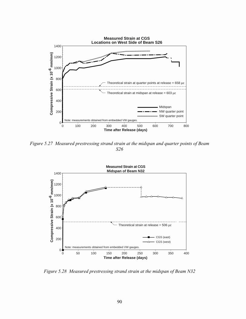
90
1400
1200
1000
800
600
400
200
0
Co
mp
ress
ive
Str
ain
(x
10-6
mm
/mm
)
Measured Strain at CGSLocations on West Side of Beam S26
Time after Release (days)0 100 200 300 400 500 600 700 800
Theoretical strain at quarter points at release = 658 µε
MidspanNW quarter pointSW quarter point
Theoretical strain at midspan at release = 603 µε
Note: measurements obtained from embedded VW gauges.
Figure 5.27 Measured prestressing strand strain at the midspan and quarter points of BeamS26
1400
1200
1000
800
600
400
200
0
Time after Release (days)0 50 100 150 200 250 300 350 400
CGS (east)
CGS (west)
Measured Strain at CGSMidspan of Beam N32
Co
mp
ress
ive
Str
ain
(x
10-6
mm
/mm
)
Theoretical strain at release = 506 µε
Note: measurements obtained from embedded VW gauges.
Figure 5.28 Measured prestressing strand strain at the midspan of Beam N32
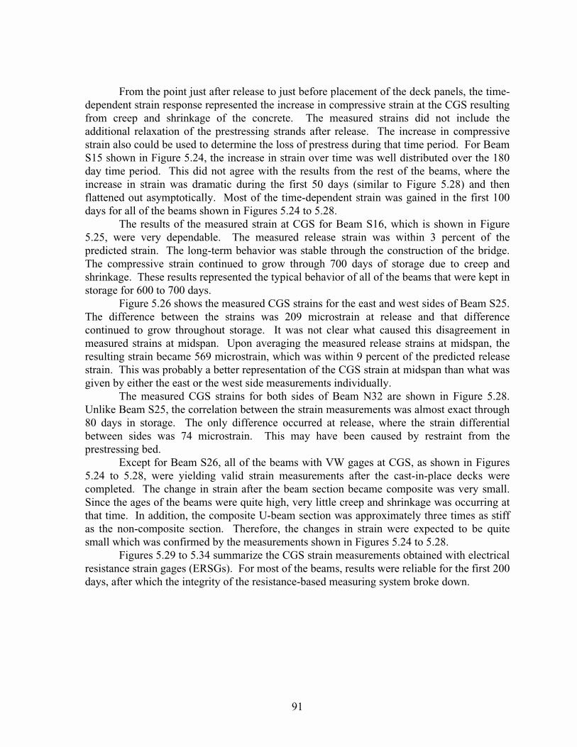
91
From the point just after release to just before placement of the deck panels, the time-dependent strain response represented the increase in compressive strain at the CGS resultingfrom creep and shrinkage of the concrete. The measured strains did not include theadditional relaxation of the prestressing strands after release. The increase in compressivestrain also could be used to determine the loss of prestress during that time period. For BeamS15 shown in Figure 5.24, the increase in strain over time was well distributed over the 180day time period. This did not agree with the results from the rest of the beams, where theincrease in strain was dramatic during the first 50 days (similar to Figure 5.28) and thenflattened out asymptotically. Most of the time-dependent strain was gained in the first 100days for all of the beams shown in Figures 5.24 to 5.28.
The results of the measured strain at CGS for Beam S16, which is shown in Figure5.25, were very dependable. The measured release strain was within 3 percent of thepredicted strain. The long-term behavior was stable through the construction of the bridge.The compressive strain continued to grow through 700 days of storage due to creep andshrinkage. These results represented the typical behavior of all of the beams that were kept instorage for 600 to 700 days.
Figure 5.26 shows the measured CGS strains for the east and west sides of Beam S25.The difference between the strains was 209 microstrain at release and that differencecontinued to grow throughout storage. It was not clear what caused this disagreement inmeasured strains at midspan. Upon averaging the measured release strains at midspan, theresulting strain became 569 microstrain, which was within 9 percent of the predicted releasestrain. This was probably a better representation of the CGS strain at midspan than what wasgiven by either the east or the west side measurements individually.
The measured CGS strains for both sides of Beam N32 are shown in Figure 5.28.Unlike Beam S25, the correlation between the strain measurements was almost exact through80 days in storage. The only difference occurred at release, where the strain differentialbetween sides was 74 microstrain. This may have been caused by restraint from theprestressing bed.
Except for Beam S26, all of the beams with VW gages at CGS, as shown in Figures5.24 to 5.28, were yielding valid strain measurements after the cast-in-place decks werecompleted. The change in strain after the beam section became composite was very small.Since the ages of the beams were quite high, very little creep and shrinkage was occurring atthat time. In addition, the composite U-beam section was approximately three times as stiffas the non-composite section. Therefore, the changes in strain were expected to be quitesmall which was confirmed by the measurements shown in Figures 5.24 to 5.28.
Figures 5.29 to 5.34 summarize the CGS strain measurements obtained with electricalresistance strain gages (ERSGs). For most of the beams, results were reliable for the first 200days, after which the integrity of the resistance-based measuring system broke down.
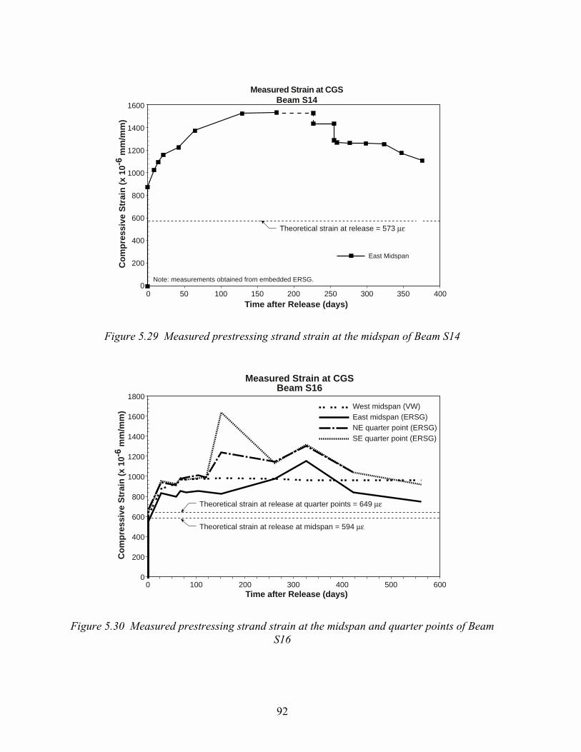
92
1600
1400
1200
1000
800
600
400
200
0
Time after Release (days)0 50 100 150 200 250 300 350 400
East Midspan
Measured Strain at CGSBeam S14
Co
mp
ress
ive
Str
ain
(x
10-6
mm
/mm
)
Theoretical strain at release = 573 µε
Note: measurements obtained from embedded ERSG.
Figure 5.29 Measured prestressing strand strain at the midspan of Beam S14
1800
1600
1400
1200
1000
800
600
400
200
0
Co
mp
ress
ive
Str
ain
(x
10-6
mm
/mm
)
Measured Strain at CGSBeam S16
Time after Release (days)0 100 200 300 400 500 600
Theoretical strain at release at quarter points = 649 µε
West midspan (VW)East midspan (ERSG)NE quarter point (ERSG)SE quarter point (ERSG)
Theoretical strain at release at midspan = 594 µε
Figure 5.30 Measured prestressing strand strain at the midspan and quarter points of BeamS16

93
1800
1600
1400
1200
1000
800
600
400
200
0
Co
mp
ress
ive
Str
ain
(x
10-6
mm
/mm
)
Measured Strain at CGSBeam S25
Time after Release (days)0 50 100 150 200 250 300 350 400 450 500
Theoretical strain at release at quarter points = 586 µε
West midspan (VW)East midspan (VW)NW quarter point (ERSG)SW quarter point (ERSG)SE quarter point (ERSG)
Theoretical strain at release at midspan = 523 µε
Figure 5.31 Measured prestressing strand strain at midspan and quarter points of Beam S25
1600
1400
1200
1000
800
600
400
200
0
Co
mp
ress
ive
Str
ain
(x
10-6
mm
/mm
)
Measured Strain at CGSBeam N21
Time after Release (days)0 50 100 150 200 250 300 350 400 450 500 550
West midspanEast midspan
Theoretical strain at release = 642 µε
Note: measurements obtained from embedded ERSGs.
Figure 5.32 Measured prestressing strand strain at the midspan of Beam N21

94
1600
1400
1200
1000
800
600
400
200
0
Co
mp
ress
ive
Str
ain
(x
10-6
mm
/mm
)
Measured Strain at CGSBeam N22
Time after Release (days)0 100 200 300 400 500 600 700
Theoretical strain at releaseat quarter points = 615 µε
East midspanNW quarter pointSE quarter point
Theoretical strain at releaseat midspan = 545 µε
Note: measurements obtained from embedded ERSGs.
Figure 5.33 Measured prestressing strand strain at midspan and quarter points of BeamN22
1800
1600
1400
1200
1000
800
600
400
200
0
Co
mp
ress
ive
Str
ain
(x
10-6
mm
/mm
)
Measured Strain at CGSBeam N31
Time after Release (days)0 100 200 300 400 500 600 700
Theoretical strain at releaseat quarter points = 679 µε
West midspanNW quarter pointSW quarter pointSE quarter point
Theoretical strain at releaseat midspan = 621 µε
Note: measurements obtained from embedded ERSGs.
Figure 5.34 Measured prestressing strand strain at the midspan and quarter points of BeamN31

95
The strain response at midspan for Beam S14, shown in Figure 5.29, was reliablethrough completion of the deck even though the strain at release was significantly higher thanthe predicted value. At approximately 325 days, the ERSG at midspan of Beam S14 began toshow signs of breakdown. The total strain throughout storage for Beam S14 was abnormallyhigher than all of the other beams, especially when compared to the results for Beam S15,shown in Figure 5.24, which was the companion beam for Beam S14. Theoretically, thestrain responses for these beams should have been similar. Differences between Beams S14and S15 can be attributed to the type of gage used to obtain strain measurements.
The strain response at midspan of Beam N21, shown Figure 5.32, was very reliable atrelease and throughout most of the time in storage. The measured and predicted releasestrains were within 1 percent of each other. The compressive strain increased throughout thefirst 250 days of storage and then decreased slightly at 300 days. After 300 days, no furthermeasurements were provided bythat gage.
The measured strains at CGS for Beam N22 are shown in Figure 5.33. The strainbehavior was stable up to 100 days, after which the strain measurements became very erratic.The strain responses that were measured with ERSGs for Beams S16 and N31, which areshown in Figures 5.30 and 5.34, respectively, showed behavior that was similar to the resultsfor Beam N22. The strain measurements obtained with ERSGs were not reliable past 200days for almost all of the beams.
Figures 5.30 compares the measured CGS strains using a VW gage at midspan to themeasured strains using ERSGs at midspan and the quarter points for Beam S16. The strainbehavior at most locations along the beam was reliable through 150 days for Beam S16. Thequarter point strains were higher than the midspan strains and the strain increase during thattime was similar for both types of gages. However, the quarter point and midspan strainmeasurements made with ERSGs past 150 days became erratic. Similar patterns of erraticresponse from ERSGs are illustrated in Beams S25, N22, and N31, shown in Figures 5.31,5.33, and 5.34, respectively. These comparisons illustrated that the VW gages yielded farmore reliable long-term strain measurements. The ERSGs consistently yielded reliableresults for much shorter periods of time and then generally became unstable.
5.3.4 Measured Strain Profiles at Midspan
Strain profiles at midspan were measured for nine of the twelve instrumented beamsusing internal strain gages, Demec surface strain gages, or a combination of both types ofgages. The measured strain profiles at midspan were of interest for determining theimmediate midspan curvatures at release as well as the time-dependent increases in curvaturethroughout storage. The curvatures at release could be compared to the measured cambers atrelease to determine whether a correlation existed between the two sets of measurements.
The measured strain profiles at release are shown in Figures 5.35 to 5.43. Thepredicted strain profiles at release were included in these figures for comparison purposes.The predicted profiles were calculated based on the same assumptions that were used tocalculate the theoretical strains at the CGS in Sec. 5.3.3.
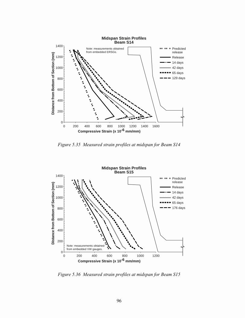
96
1400
1200
1000
800
600
400
200
0
Dis
tanc
e fr
om B
otto
m o
f Sec
tion
(mm
)
Midspan Strain ProfilesBeam S14
Compressive Strain (x 10-6 mm/mm)0 200 400 600 800 1000 1200 1400 1600
Note: measurements obtainedfrom embedded ERSGs.
Predictedrelease
Release
14 days
42 days
65 days
129 days
Figure 5.35 Measured strain profiles at midspan for Beam S14
1400
1200
1000
800
600
400
200
0
Dis
tanc
e fr
om B
otto
m o
f Sec
tion
(mm
)
Midspan Strain ProfilesBeam S15
Compressive Strain (x 10-6 mm/mm)
0 200 400 600 800 1000 1200
Note: measurements obtainedfrom embedded VW gauges.
Predictedrelease
Release
14 days
42 days
65 days
176 days
Figure 5.36 Measured strain profiles at midspan for Beam S15

97
1400
1200
1000
800
600
400
200
0
Dis
tanc
e fr
om B
otto
m o
f Sec
tion
(mm
)
Midspan Strain ProfilesBeam S16
Compressive Strain (x 10-6 mm/mm)
0 200 400 600 800 1000 1200
Note: measurements obtainedfrom embedded ERSGs.
Predictedrelease
Release
28 days
59 days
262 days
327 days
Figure 5.37 Measured strain profiles at midspan for Beam S16
1400
1200
1000
800
600
400
200
0
Dis
tanc
e fr
om B
otto
m o
f Sec
tion
(mm
)
Midspan Strain ProfilesBeam S25
Compressive Strain (x 10-6 mm/mm)
0 200 400 600 800 1000 1200
Note: measurementsobtained from embeddedVW gauges.
Predictedrelease
Release
6 days
18 days
62 days
110 days
221 days
Figure 5.38 Measured strain profiles at midspan for Beam S25

98
1400
1200
1000
800
600
400
200
0
Dis
tanc
e fr
om B
otto
m o
f Sec
tion
(mm
)
Midspan Strain ProfilesBeam S26
Compressive Strain (x 10-6 mm/mm)
0 200 400 600 800 1000 1200
Note: measurementsobtained from Demecmechanical gauges.
Predictedrelease
Release
(West)
Figure 5.39 Measured strain profiles at midspan for Beam S26
1400
1200
1000
800
600
400
200
0
Dis
tanc
e fr
om B
otto
m o
f Sec
tion
(mm
)
Midspan Strain ProfilesBeam N21
Compressive Strain (x 10-6 mm/mm)0 200 400 600 800 1000 1200 1400
Note: measurements obtainedfrom embedded ERSGs.
Predictedrelease
Release(ERSGs)
Release(Surfacestrain)
11 days
31 days
123 days
Figure 5.40 Measured strain profiles at midspan for Beam N21
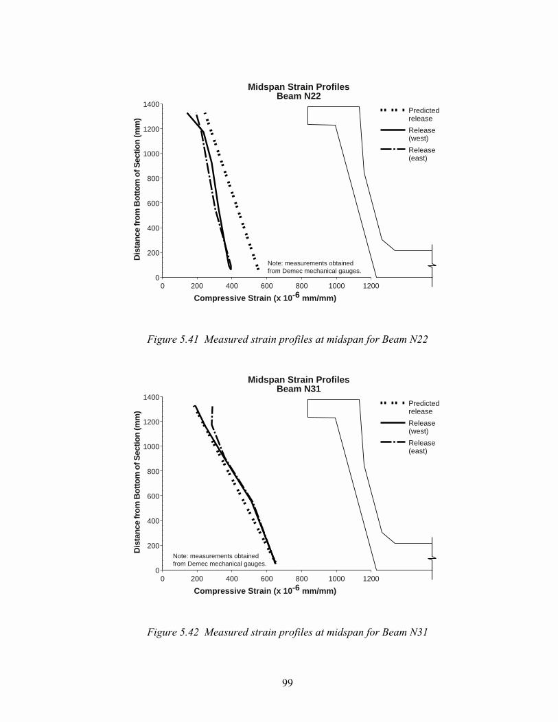
99
1400
1200
1000
800
600
400
200
0
Dis
tanc
e fr
om B
otto
m o
f Sec
tion
(mm
)
Midspan Strain ProfilesBeam N22
Compressive Strain (x 10-6 mm/mm)
0 200 400 600 800 1000 1200
Note: measurements obtainedfrom Demec mechanical gauges.
Predictedrelease
Release(west)
Release(east)
Figure 5.41 Measured strain profiles at midspan for Beam N22
1400
1200
1000
800
600
400
200
0
Dis
tanc
e fr
om B
otto
m o
f Sec
tion
(mm
)
Midspan Strain ProfilesBeam N31
Compressive Strain (x 10-6 mm/mm)
0 200 400 600 800 1000 1200
Note: measurements obtainedfrom Demec mechanical gauges.
Predictedrelease
Release(west)
Release(east)
Figure 5.42 Measured strain profiles at midspan for Beam N31
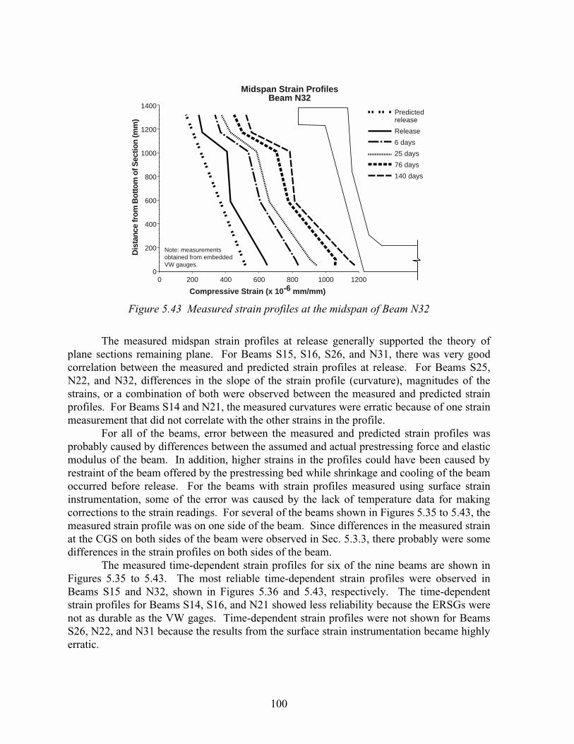
100
1400
1200
1000
800
600
400
200
0
Dis
tanc
e fr
om B
otto
m o
f Sec
tion
(mm
)
Midspan Strain ProfilesBeam N32
Compressive Strain (x 10-6 mm/mm)
0 200 400 600 800 1000 1200
Note: measurementsobtained from embeddedVW gauges.
Predictedrelease
Release
6 days
25 days
76 days
140 days
Figure 5.43 Measured strain profiles at the midspan of Beam N32
The measured midspan strain profiles at release generally supported the theory ofplane sections remaining plane. For Beams S15, S16, S26, and N31, there was very goodcorrelation between the measured and predicted strain profiles at release. For Beams S25,N22, and N32, differences in the slope of the strain profile (curvature), magnitudes of thestrains, or a combination of both were observed between the measured and predicted strainprofiles. For Beams S14 and N21, the measured curvatures were erratic because of one strainmeasurement that did not correlate with the other strains in the profile.
For all of the beams, error between the measured and predicted strain profiles wasprobably caused by differences between the assumed and actual prestressing force and elasticmodulus of the beam. In addition, higher strains in the profiles could have been caused byrestraint of the beam offered by the prestressing bed while shrinkage and cooling of the beamoccurred before release. For the beams with strain profiles measured using surface straininstrumentation, some of the error was caused by the lack of temperature data for makingcorrections to the strain readings. For several of the beams shown in Figures 5.35 to 5.43, themeasured strain profile was on one side of the beam. Since differences in the measured strainat the CGS on both sides of the beam were observed in Sec. 5.3.3, there probably were somedifferences in the strain profiles on both sides of the beam.
The measured time-dependent strain profiles for six of the nine beams are shown inFigures 5.35 to 5.43. The most reliable time-dependent strain profiles were observed inBeams S15 and N32, shown in Figures 5.36 and 5.43, respectively. The time-dependentstrain profiles for Beams S14, S16, and N21 showed less reliability because the ERSGs werenot as durable as the VW gages. Time-dependent strain profiles were not shown for BeamsS26, N22, and N31 because the results from the surface strain instrumentation became highlyerratic.

101
Beams S15, shown in Figure 5.36, was a good example of how the strain profile atmidspan changed with time owing to creep and shrinkage. The effects of creep andshrinkage on the strain profile were shown by variable increases in the magnitudes of thestrains in the cross section. Shrinkage caused a uniform increase in all of the strains whilecreep caused the strain at each location in the profile to increase in proportion to itsmagnitude at release. At 176 days, all of the strains had increased in magnitude and the slopeof the strain profile, or curvature, had increased with respect to the curvature at release. Themeasured increase in curvature for Beam S15 was expected to be accompanied by a measuredincrease in camber. The time-dependent camber response for Beam S15, shown in Figure5.17, verified the measured curvature response shown in Figure 5.36. Beam N32 displayedbehavior that was similar to Beam S15.
5.3.5 Temperature Gradients
Temperature gradients are nonuniform vertical distributions of temperature thatdevelop as a result of uneven heating and cooling. Heat energy is provided to a beam or abridge superstructure by means of solar radiation. Additional heat may be gained or lostowing to convection to or from the surrounding atmosphere. The amount of temperaturechange created by these heat sources depends upon wind speed, ambient temperature, relativehumidity, weather conditions (clear or cloudy), material properties of the bridge, surfacecharacteristics, the time of day, and the time of year (53,54,55). Maximum temperaturegradients can be expected during times of very high solar radiation and very low wind speed(54). Conditions such as these would most likely occur in the summer. At that time of theyear, the distance of the sun from the earth is the smallest and the angle of the sun relative tothe earth is the largest.
Temperatures distributions in the beams and composite bridge were measured todetermine the temperature gradient variation throughout the day and year as well as themaximum gradient that could be expected in the bridge. The magnitude of a temperaturegradient was taken as the temperature difference between the top and bottom flanges. Themeasured temperature gradients were also used to correlate predicted and observed thermallyinduced movements in the beams. This will be discussed in Sec. 5.3.6.
Temperature gradients in the beams varied significantly while they were in storage.The temperature gradients in storage were primarily used for making analytical corrections tothe camber measurements, which is discussed in Sec. 5.3.1. It is important to note that alltemperature data presented for the U-beams corresponds to typical weather patterns that existin the southeast region of Texas.
Figures 5.44 and 5.45 show typical variations in temperature distribution in the beamsduring the day while they were in storage at the prestressing plant. Temperature gradientswere typically uniform or slightly negative during the morning hours just before sunrise. Anegative temperature gradient was characterized by a temperature decrease from bottom totop of the section. In general, temperature gradients were nonlinear during sunny afternoonswith temperature differences between the top and bottom flanges ranging from 7 to 10 �C.The nonlinear shape of the temperature gradient, as shown in Figure 5.45, was due to shading

102
of the web by the top flange. This shading caused the upper part of the web to remainslightly cooler than the lower part of the web. The lower flange heated and cooled moreslowly than the rest of the beam because of its large mass.
1400
1200
1000
800
600
400
200
0
Dis
tan
ce f
rom
Bo
tto
m o
f B
eam
(m
m)
Temperature Gradients on November 29, 1994
Temperature (°C)
10 15 20 25 30 35
8:30 amCloudy, 16°C
12:45 pmPartly Cloudy,24°C
4:00 pmSunny, 24°C
Beam S16(in storage)
Figure 5.44 Temperature distributions at midspan on a mostly cloudy fall day
1400
1200
1000
800
600
400
200
0
Dis
tan
ce f
rom
Bo
tto
m o
f B
eam
(m
m)
Temperature Gradients on August 24, 1995
Temperature (°C)20 25 30 35 40 45 50
10:00 amSunny
1:15 pmSunny
4:00 pmSunny
5:15 pmSunny
Beam N21(in storage)
Figure 5.45 Temperature distributions at midspan on a hot summer day

103
Figure 5.44 shows how temperature distributions changed on November 29, 1994,which was a mostly cloudy fall day. The temperature gradient changed from -1 �C at 8:30a.m. to 5 �C by 4:00 p.m. The shape of the temperature gradient became highly nonlinear inthe afternoon as the weather conditions changed from cloudy to sunny.
Figure 5.45 shows the variation in temperature distribution in Beam N21 on August24, 1995, which was a hot sunny summer day. At 10:00 a.m., the measured temperaturedistribution was nearly uniform. By 1:15 p.m., the beam had heated up considerably with thetop flange and lower web experiencing a larger increase in temperature than the upper weband lower flange. The temperature distribution had assumed the characteristic nonlinearshape by that time. The temperature gradient reached a maximum of 7 �C by 4:00 p.m. Thislarge temperature gradient lasted all afternoon with the peak beam temperatures occurringbetween 5 p.m. and 6 p.m.
Temperature distributions in the composite bridge were of more interest than thosemeasured while the beams were in storage. The measurement of temperatures in thecomposite bridge were important for determining variations in temperature gradientsthroughout the day and the year, and for determining the maximum gradient that could beexpected in the composite section. The maximum temperature gradients observed in thecomposite section between November of 1996 and March of 1997 was 12 �C. The maximumchange in temperature in the deck during a single day was 19 �C.
Figures 5.46 through 5.49 show the large nonlinear temperature gradients that weremeasured in the composite U-beam sections. Figures 5.46 and 5.48 show the variation oftemperature gradients in Beam N21, which was an exterior beam. Figures 5.47 and 5.49show the variation of temperature gradients for Beam N33, which was an interior beam.These beams were used to represent typical temperature distributions in exterior and interiorcomposite U-beams. The positions of these beams in the bridge are shown in Sec. 3.2.1.There will be some variation among similar beams based on their position in the bridge andbased on the thickness of the deck slab.
Figures 5.46 and 5.47 show the temperature gradients that developed in Beams N21and N33, respectively, on March 10, 1997, which appeared to be a hot and sunny day. Thetemperature distributions early in the morning were generally uniform or slightly negative forboth beams with the deck being cooler than the bottom flange. From 8:00 a.m. to 12:00 p.m.,the temperature in the deck had increased by 7 �C and 9 �C for Beams N21 and N33,respectively. During the same period of time, the lower part of Beam N21 had increaseduniformly by 3 �C while the lower part of Beam N33 remained almost the same temperature.By 3:00 p.m., the temperature gradient in Beam N21 was 6 �C (13 �C increase at the top and7 �C increase at the bottom flange) while the temperature gradient in Beam N33 was 9 �C (13�C increase at the top and 4 �C increase at the bottom flange). The portion of Beam N33below the top flange increased uniformly by a smaller amount than Beam N21 because of thecomplete shading of the interior beam from the sun.
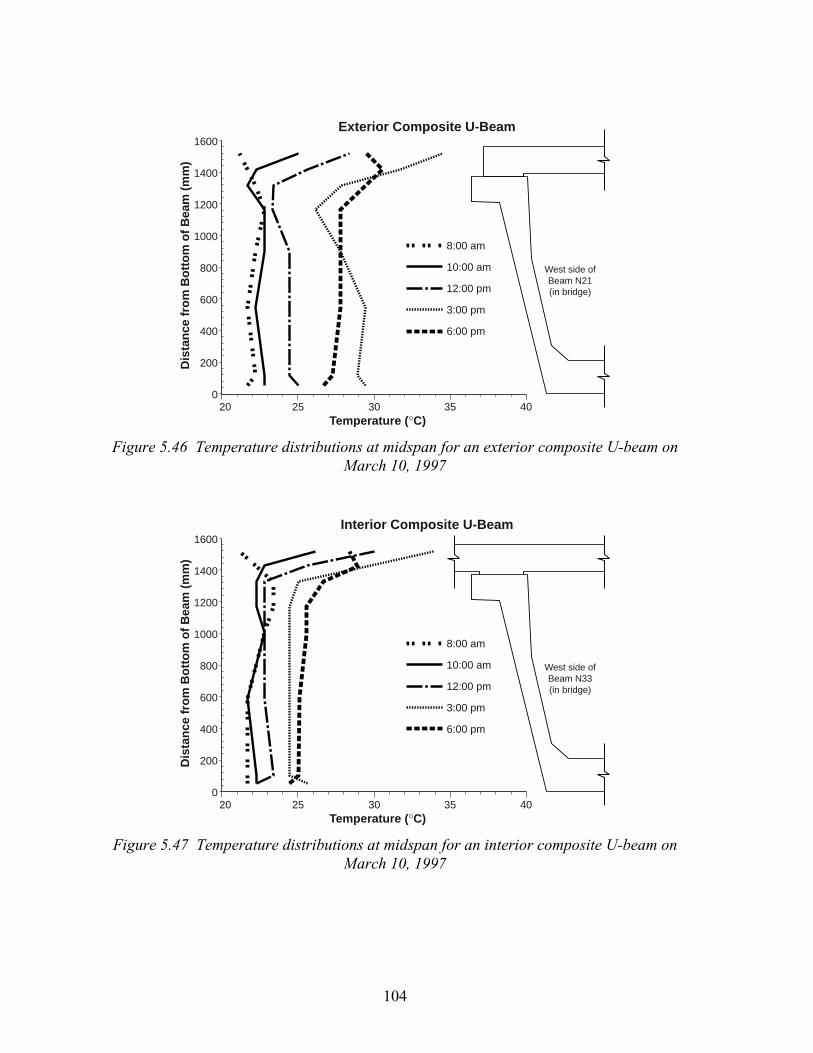
104
1600
1400
1200
1000
800
600
400
200
0
Dis
tan
ce f
rom
Bo
tto
m o
f B
eam
(m
m)
Exterior Composite U-Beam
Temperature (°C)20 25 30 35 40
8:00 am
10:00 am
12:00 pm
3:00 pm
6:00 pm
West side ofBeam N21(in bridge)
Figure 5.46 Temperature distributions at midspan for an exterior composite U-beam onMarch 10, 1997
1600
1400
1200
1000
800
600
400
200
0
Dis
tan
ce f
rom
Bo
tto
m o
f B
eam
(m
m)
Interior Composite U-Beam
Temperature (°C)20 25 30 35 40
8:00 am
10:00 am
12:00 pm
3:00 pm
6:00 pm
West side ofBeam N33(in bridge)
Figure 5.47 Temperature distributions at midspan for an interior composite U-beam onMarch 10, 1997

105
1600
1400
1200
1000
800
600
400
200
0
Dis
tan
ce f
rom
Bo
tto
m o
f B
eam
(m
m)
Exterior Composite U-Beam
Temperature (°C)0 5 10 15 20 25
8:00 am
10:00 am
12:00 pm
2:00 pm
4:00 pm
West side ofBeam N21(in bridge)
Figure 5.48 Temperature distributions at midspan for an exterior composite U-beam onJanuary 30, 1997
1600
1400
1200
1000
800
600
400
200
0
Dis
tan
ce f
rom
Bo
tto
m o
f B
eam
(m
m)
Interior Composite U-Beam
Temperature (°C)0 5 10 15 20
8:00 am
10:00 am
12:00 pm
2:00 pm
4:00 pm
West side ofBeam N33(in bridge)
Figure 5.49 Temperature distributions at midspan for an interior composite U-beam onJanuary 30, 1997
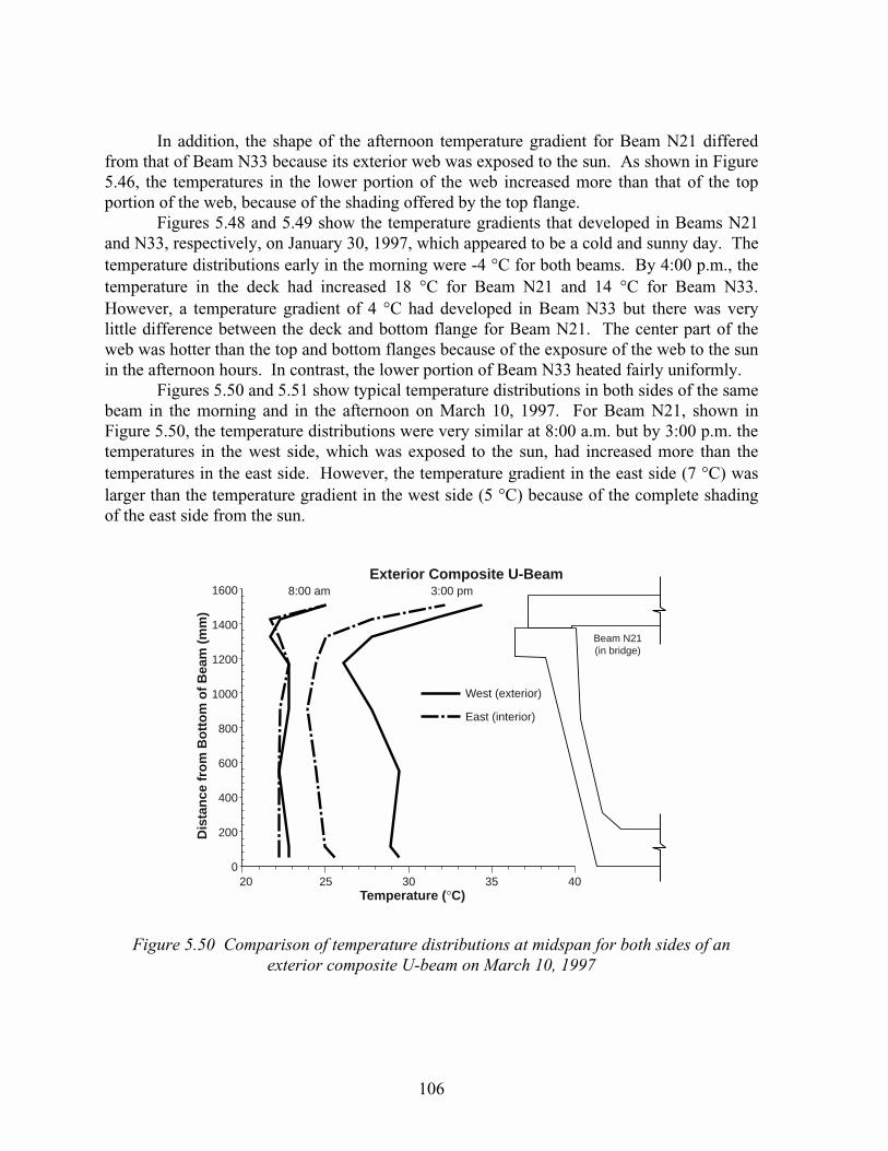
106
In addition, the shape of the afternoon temperature gradient for Beam N21 differedfrom that of Beam N33 because its exterior web was exposed to the sun. As shown in Figure5.46, the temperatures in the lower portion of the web increased more than that of the topportion of the web, because of the shading offered by the top flange.
Figures 5.48 and 5.49 show the temperature gradients that developed in Beams N21and N33, respectively, on January 30, 1997, which appeared to be a cold and sunny day. Thetemperature distributions early in the morning were -4 �C for both beams. By 4:00 p.m., thetemperature in the deck had increased 18 �C for Beam N21 and 14 �C for Beam N33.However, a temperature gradient of 4 �C had developed in Beam N33 but there was verylittle difference between the deck and bottom flange for Beam N21. The center part of theweb was hotter than the top and bottom flanges because of the exposure of the web to the sunin the afternoon hours. In contrast, the lower portion of Beam N33 heated fairly uniformly.
Figures 5.50 and 5.51 show typical temperature distributions in both sides of the samebeam in the morning and in the afternoon on March 10, 1997. For Beam N21, shown inFigure 5.50, the temperature distributions were very similar at 8:00 a.m. but by 3:00 p.m. thetemperatures in the west side, which was exposed to the sun, had increased more than thetemperatures in the east side. However, the temperature gradient in the east side (7 �C) waslarger than the temperature gradient in the west side (5 �C) because of the complete shadingof the east side from the sun.
8:00 am 3:00 pm1600
1400
1200
1000
800
600
400
200
0
Dis
tan
ce f
rom
Bo
tto
m o
f B
eam
(m
m)
Exterior Composite U-Beam
Temperature (°C)20 25 30 35 40
West (exterior)
East (interior)
Beam N21(in bridge)
Figure 5.50 Comparison of temperature distributions at midspan for both sides of anexterior composite U-beam on March 10, 1997

107
8:00 am 4:00 pm1600
1400
1200
1000
800
600
400
200
0
Dis
tan
ce f
rom
Bo
tto
m o
f B
eam
(m
m)
Interior Composite U-Beam
Temperature (°C)15 20 25 30 35 40
Beam S15(in bridge)
East
West
Figure 5.51 Comparison of temperature distributions at midspan for both sides of aninterior composite U-beam on March 9, 1997
Figure 5.51 shows a similar comparison for Beam S15, which was an interior beam.The temperature data shown was from March 9, 1997. The temperature distributions in bothsides of Beam S15 were nearly identical at 8:00 a.m. By 4:00 p.m., both temperaturedistributions became highly nonlinear but there was very little difference between thetemperature gradients that developed in both sides of the beam. Since both sides werecompletely shaded from the sun, there was no influence that caused the temperaturedistributions to vary between the two sides of the beams.
5.3.6 Thermally Induced Camber and Deflection
Thermal movements in prestressed concrete beams occur as both axial and flexuraldeformations. Axial lengthening or shortening occurs when a beam is uniformly heated orcooled, respectively. If a beam is allowed to expand or contract freely, camber or deflectionwill not be induced in the beam by this type of deformation. Flexural deformations arecaused by nonuniform temperature distributions throughout the depth of the beam crosssection. When a simply supported beam is subjected to nonuniform temperaturedistributions, a resulting thermally induced camber or deflection will occur in the beam (53).
Changes in camber resulting from temperature gradients were measured for BeamsN21 and S16 during storage and for the beams in spans two and three of the northbound mainlanes bridge after the composite deck was completed. The locations of these beams in thebridge are shown in Figures 3.2 and 3.3 in Section 3.2.1. These measurements aresummarized in Tables 5.3 to 5.6. Camber measurements were taken throughout the day toobserve the increase in camber resulting from temperature gradients in the beam. The firstcamber measurements were taken in the morning and were used as the baseline reading.Thermal movements were determined by subtracting the initial camber measurement fromthe measurement later in the day. It was assumed that no time-dependent changes in camberoccurred during the times that the measurements were taken.

108
Table 5.3 shows the measured thermal movements for Beam N21 on August 24,1995. The maximum measured increase in camber was 8.6 mm at 2:45 p.m. Several of themeasured temperature gradients for Beam N21 on that day are shown in Figure 5.45.Predicted changes in camber based on these gradients were calculated and included in Table5.3 for comparison with the measured changes in camber. The predicted thermal movementswere calculated as described in Section 5.3.1. The maximum theoretical increase in camberwas 10.7 mm at 3:50 p.m. The predictions tended to overestimate the measured thermalmovements throughout the afternoon. Incorrect assumptions in the theoretical model,unequal heating of the two sides of the beam, and variation of the temperature gradient alongthe length of the beam could have been possible causes for the overestimations of camberresulting from thermal movements. The theoretical model was very sensitive to thetemperature of the bottom flange since it had such a large mass relative to the whole section.Small errors in the bottom flange temperature caused large variations in the estimatedthermal movement.
Table 5.3 Measured thermal movements on August 24, 1995 for Beam N21 in storage
Time Weather ConditionsMeasured Change in
Camber (mm)Predicted Change in
Camber (mm)2
10:10 a.m.1 Sunny 0.0 0.011:00 a.m. Sunny 3.6 0.31:05 p.m. Sunny 7.1 7.62:45 p.m. Sunny 8.6 9.73:50 p.m. Sunny 8.4 10.75:10 p.m. Sunny 6.6 9.9
Notes:1.� The measurement taken at this time was considered the baseline reading.2.� Predicted changes in camber were calculated based on the measured temperature gradients
for Beam N21 as shown in Fig. 5.45.
Table 5.4 shows the measured thermal movements for Beam S16 on November 29,1994. The measured camber grew 11.4 mm by 4:00 p.m. as the day turned from cloudy tosunny. The measured temperature gradients for Beam S16 on that day are shown in Figure5.44. For this beam, the measured changes in camber were larger than the predicted changesin camber. The probable causes for these differences are the same as those identified for theresults of Beam N21.
These two days were the only times that thermal movements were measuredthroughout the course of a day for beams in storage. Because of the limited amount of data,the maximum camber caused by temperature gradients for 40-meter long U-beams in storagecannot be determined. Based on the data available, as summarized above, the expectedthermally induced camber should be at least 11.4 mm.
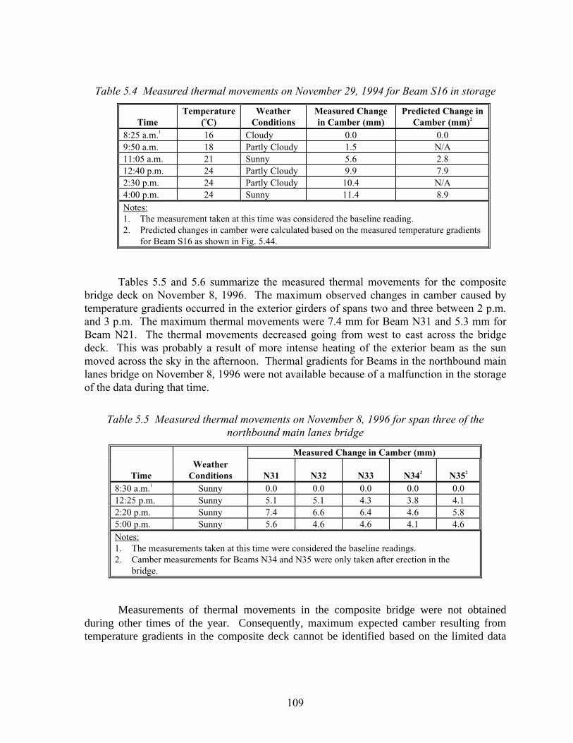
109
Table 5.4 Measured thermal movements on November 29, 1994 for Beam S16 in storage
TimeTemperature
(oC)Weather
ConditionsMeasured Changein Camber (mm)
Predicted Change inCamber (mm)2
8:25 a.m.1 16 Cloudy 0.0 0.09:50 a.m. 18 Partly Cloudy 1.5 N/A11:05 a.m. 21 Sunny 5.6 2.812:40 p.m. 24 Partly Cloudy 9.9 7.92:30 p.m. 24 Partly Cloudy 10.4 N/A4:00 p.m. 24 Sunny 11.4 8.9Notes:1.� The measurement taken at this time was considered the baseline reading.2.� Predicted changes in camber were calculated based on the measured temperature gradients
for Beam S16 as shown in Fig. 5.44.
Tables 5.5 and 5.6 summarize the measured thermal movements for the compositebridge deck on November 8, 1996. The maximum observed changes in camber caused bytemperature gradients occurred in the exterior girders of spans two and three between 2 p.m.and 3 p.m. The maximum thermal movements were 7.4 mm for Beam N31 and 5.3 mm forBeam N21. The thermal movements decreased going from west to east across the bridgedeck. This was probably a result of more intense heating of the exterior beam as the sunmoved across the sky in the afternoon. Thermal gradients for Beams in the northbound mainlanes bridge on November 8, 1996 were not available because of a malfunction in the storageof the data during that time.
Table 5.5 Measured thermal movements on November 8, 1996 for span three of thenorthbound main lanes bridge
Measured Change in Camber (mm)
TimeWeather
Conditions N31 N32 N33 N342 N352
8:30 a.m.1 Sunny 0.0 0.0 0.0 0.0 0.012:25 p.m. Sunny 5.1 5.1 4.3 3.8 4.12:20 p.m. Sunny 7.4 6.6 6.4 4.6 5.85:00 p.m. Sunny 5.6 4.6 4.6 4.1 4.6Notes:1.� The measurements taken at this time were considered the baseline readings.2.� Camber measurements for Beams N34 and N35 were only taken after erection in the
bridge.
Measurements of thermal movements in the composite bridge were not obtainedduring other times of the year. Consequently, maximum expected camber resulting fromtemperature gradients in the composite deck cannot be identified based on the limited data

110
presented here. The maximum thermal movements for this composite bridge can be expectedto be at least 7.4 mm.
Table 5.6 Measured thermal movements on November 8, 1996 for span two of thenorthbound main lanes bridge
Measured Change in Camber (mm)
TimeWeather
Conditions N21 N22 N238:20 a.m.1 Sunny 0.0 0.0 0.012:10 p.m. Sunny 4.1 3.6 3.32:40 p.m. Sunny 5.3 5.1 5.15:20 p.m. Sunny 4.8 3.6 3.8�
� Notes: 1. The measurements taken at this time were considered the baseline readings.�
5.4 COMPARISON OF MEASURED BEHAVIOR
5.4.1 Camber and Deflection
Measured camber and deflection responses for the twelve instrumented beams werecompared to identify similarities and differences in behavior among the beams. Comparisonof time-dependent camber responses were made between sets of companion beams that hadnearly identical properties. Further comparisons were made among all of the beams toexamine differences between measured and predicted elastic cambers at release, growth incamber from release to just before placement of the deck panels, and correlation of measuredelastic responses to superimposed loads among beams in the same span.
5.4.1.1 Camber Responses for Companion Beams
The time-dependent camber plots shown in Sec. 5.3.1 can be compared to one anotherbecause many of the beams shared similar casting dates, section types, span lengths, andstrand patterns. The camber responses for four pairs of beams are shown in Figures 5.52 to5.55 to examine whether the companion beams behaved similarly.
Figure 5.52 shows the time-dependent camber responses for Beams N32 and N33,which were cast on February 15, 1996. Both beams were U54A cross sections having 64prestressing strands. The span length during storage for Beam N32 was only 0.20 meters lessthan the span length of Beam N33. The beams were positioned next to one another in spanthree of the northbound bridge. The span length in the bridge for Beam N32 was only 0.16meters less than the span length for Beam N33. The camber responses for both of the beamswere adjusted for thermally induced camber and support conditions during storage.
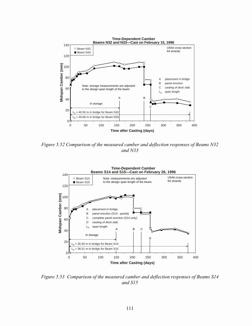
111
140
120
100
80
60
40
20
0
Mid
span
Cam
ber
(m
m)
Time after Casting (days)
0 50 100 150 200 250 300 350 400
Beam N32Beam N33
In storage
A B
Time-Dependent CamberBeams N32 and N33—Cast on February 15, 1996
A placement in bridge
B panel erection
C casting of deck slab
Ls span length
C
Ls = 40.50 m in bridge for Beam N32
U54A cross-section64 strands
Ls = 40.66 m in bridge for Beam N33
Note: storage measurements are adjustedto the design span length of the beam.
Figure 5.52 Comparison of the measured camber and deflection responses of Beams N32and N33
140
120
100
80
60
40
20
0
Mid
span
Cam
ber
(m
m)
Time after Casting (days)
0 50 100 150 200 250 300 350 400
Beam S14Beam S15
In storage
A C
Time-Dependent CamberBeams S14 and S15—Cast on February 26, 1996
A placement in bridge
B panel erection (S14 - partial)
C complete panel erection (S14 only)
D casting of deck slab
Ls span length
D
Ls = 35.55 m in bridge for Beam S14
U54A cross-section64 strands
Ls = 36.01 m in bridge for Beam S15
Note: measurements are adjustedto the design span length of the beam.
B
Figure 5.53 Comparison of the measured camber and deflection responses of Beams S14and S15

112
120
100
80
60
40
20
0
-20
-40
Mid
span
Cam
ber
(m
m)
Time after Casting (days)
0 100 200 300 400 500 600 700 800 900 1000
Beam S24Beam S25
In storage
A
C
Time-Dependent CamberBeams S24 and S25—Cast on November 10, 1994
A placement in bridge
B panel erection
C casting of deck slab
Ls span length
Ls = 39.83 m in bridge for Beam S24
U54B cross-section68 strands
Ls = 40.33 m in bridge for Beam S25
Note: storage measurements are adjustedto the design span length of the beam.
B
Figure 5.54 Comparison of the measured camber and deflection responses of Beams S24and S25
180
160
140
120
100
80
60
40
20
0
Mid
span
Cam
ber
(m
m)
Time after Casting (days)
0 100 200 300 400 500 600 700 800 900 1000
Beam N21Beam N31
In storage
A C
Time-Dependent CamberBeams N21 and N31—Cast on October 28, 1994
A placement in bridge
B partial panel erection (Beam N21)
C complete panel erection
D casting of deck slab
Ls span length
Ls = 40.90 m in bridge for Beam N21
U54B cross-sectionBeam N21 - 87 strandsBeam N31 - 83 strands
Ls = 40.35 m in bridge for Beam N31
Note: storage measurements are adjustedto the design span length of the beam.
B D
Figure 5.55 Comparison of the measured camber and deflection responses of Beams N21and N31

113
The initial cambers at release were 63.8 mm and 65.9 mm for Beams N32 and N33,respectively. The camber for Beam N32 increased faster than for Beam N33, even thoughthe support conditions were almost identical for these two beams. The plots of the midspancamber versus time shown in Figure 5.52 have the same shape. The cambers for Beams N32and N33 just before the precast deck panels were erected were 107.7 mm and 99.8 mm,respectively. The camber in Beam N32 increased 10.0 mm more than Beam N33 over aperiod of 238 days.
Elastic responses to superimposed loads were very similar for the two beams. Whenthe precast panels were erected, Beam N32 deflected 32.0 mm while Beam N33 deflected32.7 mm. After the cast-in-place deck was poured, Beam N32 deflected 35.3 mm and BeamN33 deflected 32.0 mm. The difference between the last two measurements can be attributedto variations in the deck thickness. At 386 days after casting, a camber differential of only6.1 mm remained between the two beams. The measured camber and deflection values forall three sets of companion beams are summarized in Table 5.7.
Figure 5.53 shows the camber response histories for Beams S14 and S15. Thesebeams were also U54A cross sections with 64 prestressing strands. The design span length ofBeam S14 was 0.47 meters shorter than the design span length of Beam S15, and its spanlength in storage was 0.50 meters shorter as well. The camber responses for these beamswere much closer than for Beams N32 and N33 even though the difference in supportedlength was larger. There was virtually no camber differential between Beams S14 and S15 atrelease, after casting of the deck, and at 375 days after casting. At 375 days, the camber inBeam S14 was only 1.3 mm larger than that of Beam S15. Table 5.7 summarizes the camberand deflection values for Beams S14 and S15.
Figure 5.54 shows the camber response histories for Beams S24 and S25. Thesebeams were U54B cross sections with 68 prestressing strands. The design span length ofBeam S24 was 0.50 meters shorter than the design span length of Beam S25, and its spanlength in storage was 0.52 to 0.60 meters shorter as well. Measured camber and deflectionvalues for these beams are summarized in Table 5.7. The camber at release for Beam S24was 6.7 mm higher than for Beam S25. The camber for Beam S24 remained higher untilplacement of the deck panels. At that time, the cambers of the two beams were nearlyidentical and stayed that way through 848 days after casting. At 848 days, the camber inBeam S24 was only 0.2 mm larger than that of Beam S25.
Table 5.7 Comparison of camber and deflection responses for companion beams
Measured Camber or Deflection (mm)Time or Event N21 N31 N32 N33 S14 S15 S24 S25
Initial camber at release 80.5 78.1 63.8 65.9 61.8 62.4 50.8 44.1Camber before deck panels 136.4 132.6 107.7 99.8 98.3 101.9 84.8 85.9Deflection resulting from deck panels 27.7 24.9 32.0 32.7 29.7 30.3 36.0 38.1Deflection resulting from CIP deck 29.5 26.7 35.3 32.0 24.9 28.7 41.4 40.7Long-term camber 77.7 76.7 35.1 29.0 35.6 34.3 2.3 2.5

114
Figure 5.55 shows the camber response histories for Beams N21 and N31. Thesebeams were U54B cross sections with similar span lengths but their strand patterns wereslightly different. The strand patterns for Beams N21 and N31 contained 87 and 83 strands,respectively. Since these beams were in the same pour, four of the strands needed to bedebonded for the entire length of Beam N31.
The design span length of Beam N21 was 0.55 meters longer that of Beam N31, andits span length in storage was 0.78 to 1.08 meters longer as well. Measured camber anddeflection values for these beams are summarized in Table 5.7. The camber at release forBeam N21 was only 2.4 mm higher than for Beam N31. The camber responses for thesebeams remained nearly identical up to placement of the deck panels, at which time thecamber for Beam N21 was only 3.8 mm larger. The agreement in camber for these beamswas probably due to the slightly shorter span length of Beam N31 offsetting the slightlyhigher prestressing force of Beam N21.
The elastic deflections resulting from the deck panels and cast-in-place (CIP) deckwere very similar. The deflections observed in Beam N31 were slightly lower than those ofBeam N21 because of a shorter span length, smaller beam spacing, and possible variation inthe actual thickness of the CIP deck. At 861 days after casting, the camber in Beam N21 wasonly 1.0 mm larger than that of Beam N31. The smaller deck load deflections for Beam N31offset the slightly larger increase in camber during storage for Beam N21.
5.4.1.2 Comparison of Measured and Predicted Cambers at Release
The measured and predicted elastic cambers at release are summarized in Table 5.8.Predicted cambers at release were calculated based on the second area-moment theorem forcalculating deflections, which can be found in any mechanics of materials text. The elasticcamber response at release was comprised of a component resulting from the prestress force(upward deflection) and a component resulting from the weight of the beam (downwarddeflection). Strand debonding was considered when calculating the upward deflection causedby the prestress force. The prestress losses assumed for this calculation were 2 percent forstrand relaxation, 2 percent for temperature losses, and the immediate losses resulting fromelastic shortening. The beam diaphragms were included in the calculation of downwarddeflection resulting from the beam weight. The elastic modulus for the concrete used in thesecalculations was the measured elastic modulus at release for each beam, which is shown inSec. 5.2.2. Transformed section properties, which were calculated by transforming the strandsteel to an equivalent area of concrete, were also used for the predicted camber calculations.
Differences between measured and predicted camber at release varied considerably.All of the measured release cambers were lower than the predicted cambers. The measuredcambers ranged from 2.4 to 25.0 mm lower than the predicted values. Ratios of measuredcamber to predicted camber varied between 0.646 and 0.972. The initial cambers werereasonably well estimated, considering that the net camber was the small difference betweentwo large components of deflection, namely the upward prestress component and thedownward beam weight component.

115
For the beams that had ratios of measured camber to predicted camber greater than0.868, the lack of camber was probably resulting from some combination of the following:
1.� The measured elastic modulus was lower than the actual elastic modulus in thebeam.
2.� The actual prestress force transferred to the beam was lower than the assumedprestress force.
3.� The actual beam weight was slightly larger owing to the volume of steelembedded in the concrete.
4.� The calculation for thermally induced camber or deflection in the beams was notcorrect.
Table 5.8 Comparison of measured and predicted cambers at release
BeamMeasured
Camber (mm)Predicted
Camber (mm)Measured - Predicted
(mm)Ratio of Measured
to Predicted CamberS14 61.8 69.9 -8.1 0.884S15 62.4 69.9 -7.5 0.893S16 49.1 71.9 -22.8 0.683S24 50.8 69.3 -18.5 0.733S25 44.1 68.3 -24.2 0.646S26 84.51 86.9 -2.4 0.972N21 80.5 92.7 -12.2 0.868N22 46.4 71.4 -25.0 0.650N23 45.01 61.2 -16.2 0.735N31 78.1 89.2 -11.1 0.876N32 63.8 71.1 -7.3 0.897N33 65.9 71.1 -5.2 0.927
Notes:1.� These measurements were not adjusted for thermally induced movement.
An increase in the modulus of elasticity by 10 percent lowered the predicted cambersby 5.1 to 7.6 mm. An increase in the estimated losses before release by 2 percent lowered thepredicted cambers by 2.5 to 3.8 mm. An increase in the weight of the beam by 2 percentlowered the predicted cambers by an additional 1.3 to 2.0 mm. A combination of theseconditions could possibly change the predicted cambers by as much as 13.4 mm.
The analytical correction for thermally induced movement was very sensitive to thetemperature assigned to the bottom flange because of its large mass. In addition, thetemperatures measured at the bottom flange and CGS were assumed not to vary across thesection. Thus, small errors in the measured temperatures could have resulted in sizeablevariations in the thermal camber.
Also, the analytical correction for thermally induced movement was made based on auniform temperature gradient, as described in Sec. 5.3.1. However, temperature gradients of

116
9 �C were observed during casting for Beams S16 and N32. From that temperature gradient,a beam would cool down to a uniform temperature gradient, implying that cooling of thesection would be uneven. Since the top would cool down, or shorten, more than the bottom,a negative curvature would be induced in the beam that would cause a component ofdeflection. This component of deflection would not be observable until after release.Corrections for uneven cooling were not made because of lack of data. However, samplecalculations for Beams S16 and N32 showed that the magnitude of this component could beas large as 12 mm.
While seven of the beams had camber that was low by 12.2 mm or less, the other fivebeams had camber that was low by as much as 25.0 mm. Differences that large were notcaused by variations in elastic modulus and prestress force alone. One possible cause forthese large differences was that there were errors in the baseline camber reading for some ofthese beams. For the beams cast in 1994, which includes all five of the beams with very lowinitial camber, the baseline piano wire camber reading was taken after the plywood pads wereplaced under the ends of the beam. Therefore, corrections needed to be made to account forthe thickness of the pads. This problem was not realized until the last pour in 1994 andestimations needed to be made for the pad thickness. Corrections for the pad thickness weremade although there could have been a variation of as much as 6.4 mm between the assumedand actual pad thickness.
The baseline camber reading for the beams cast in 1996 was taken before the padswere in place. The cambers for those beams were much closer to the predicted cambers, asshown in Table 5.8.
5.4.1.3 Camber Growth During Storage
The midspan camber growth during storage for all of the instrumented beams issummarized in Table 5.9. The measured camber just before placement of the deck panelswas used to determine a ratio of long-term camber to camber at release. This was aconvenient way of comparing the camber growth for all of the beams. Shrinkage and creepof the concrete was essentially complete for all of the beams at the time of placement of thedeck panels.
The camber growth ratios were between 1.51 and 1.70 for eight of the twelve beams.The average growth ratio was 1.74. Beam S16 had the largest growth ratio at 2.08, whichwas probably a result of low initial camber. The initial camber for Beam S16 wasapproximately 12 mm lower than Beams S14 and S15 despite having four more prestressingstrands. All three beams had essentially the same span.
Out of the four sets of companion beams, only Beams S14 and S15 and Beams N21and N31 had growth ratios that were close to each other. The other two sets of companionbeams had significantly different growth ratios.
The growth ratio for Beam S26 was only 1.55 because transfer occurred at 7 days.The later age for transfer (compressive loading of the concrete owing to prestress)significantly affected the time-dependent camber growth resulting from creep. The four
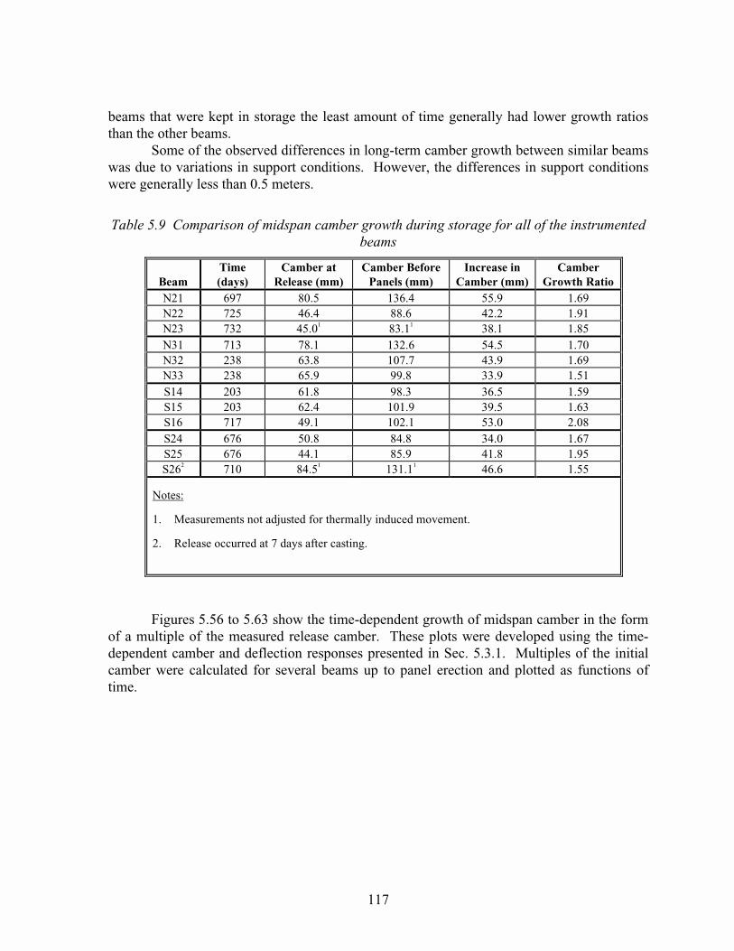
117
beams that were kept in storage the least amount of time generally had lower growth ratiosthan the other beams.
Some of the observed differences in long-term camber growth between similar beamswas due to variations in support conditions. However, the differences in support conditionswere generally less than 0.5 meters.
Table 5.9 Comparison of midspan camber growth during storage for all of the instrumentedbeams
BeamTime(days)
Camber atRelease (mm)
Camber BeforePanels (mm)
Increase inCamber (mm)
CamberGrowth Ratio
N21 697 80.5 136.4 55.9 1.69N22 725 46.4 88.6 42.2 1.91N23 732 45.01 83.11 38.1 1.85N31 713 78.1 132.6 54.5 1.70N32 238 63.8 107.7 43.9 1.69N33 238 65.9 99.8 33.9 1.51S14 203 61.8 98.3 36.5 1.59S15 203 62.4 101.9 39.5 1.63S16 717 49.1 102.1 53.0 2.08S24 676 50.8 84.8 34.0 1.67S25 676 44.1 85.9 41.8 1.95S262 710 84.51 131.11 46.6 1.55
Notes:
1.� Measurements not adjusted for thermally induced movement.
2.� Release occurred at 7 days after casting.
Figures 5.56 to 5.63 show the time-dependent growth of midspan camber in the formof a multiple of the measured release camber. These plots were developed using the time-dependent camber and deflection responses presented in Sec. 5.3.1. Multiples of the initialcamber were calculated for several beams up to panel erection and plotted as functions oftime.

118
2.0
1.9
1.8
1.7
1.6
1.5
1.4
1.3
1.2
1.1
1.0
Mu
ltip
le o
f C
amb
er a
t R
elea
se
Time after Release (days)0 100 200 300 400 500 600 700 800
Beam N21 (measured)
Beam N31 (measured)
Growth prediction (Equation 5.13)
Camber GrowthBeams N21 and N31
Figure 5.56 Camber growth ratios up to panel erection for Beams N21 and N31
2.0
1.9
1.8
1.7
1.6
1.5
1.4
1.3
1.2
1.1
1.0
Mu
ltip
le o
f C
amb
er a
t R
elea
se
Time after Release (days)0 50 100 150 200 250 300
Beam N32 (measured)
Beam N33 (measured)
Growth prediction (Equation 5.13)
Camber GrowthBeams N32 and N33
Figure 5.57 Camber growth ratios up to panel erection for Beams N32 and N33

119
2.0
1.9
1.8
1.7
1.6
1.5
1.4
1.3
1.2
1.1
1.0
Mu
ltip
le o
f C
amb
er a
t R
elea
se
Time after Release (days)0 50 100 150 200 250
Beam S14 (measured)
Beam S15 (measured)
Growth prediction (Equation 5.13)
Camber GrowthBeams S14 and S15
Figure 5.58 Camber growth ratios up to panel erection for Beams S14 and S15
2.2
2.1
2.0
1.9
1.8
1.7
1.6
1.5
1.4
1.3
1.2
1.1
1.0
Mu
ltip
le o
f C
amb
er a
t R
elea
se
Time after Release (days)0 100 200 300 400 500 600 700 800
Beam S24 (measured)
Beam S25 (measured)
Growth prediction (Equation 5.13)
Camber GrowthBeams S24 and S25
Figure 5.59 Camber growth ratios up to panel erection for Beams S24 and S25

120
2.2
2.1
2.0
1.9
1.8
1.7
1.6
1.5
1.4
1.3
1.2
1.1
1.0
Mu
ltip
le o
f C
amb
er a
t R
elea
se
Time after Release (days)0 100 200 300 400 500 600 700 800
Beam N22 (measured)
Growth prediction (Equation 5.13)
Camber GrowthBeam N22
Note: Camber measurements were not adjusted for thermal movements.
Figure 5.60 Camber growth ratios up to panel erection for Beam N22
2.0
1.9
1.8
1.7
1.6
1.5
1.4
1.3
1.2
1.1
1.0
Mu
ltip
le o
f C
amb
er a
t R
elea
se
Time after Release (days)0 100 200 300 400 500 600 700 800
Beam N23 (measured)
Growth prediction (Equation 5.13)
Camber GrowthBeam N23
Figure 5.61 Camber growth ratios up to panel erection for Beam N23
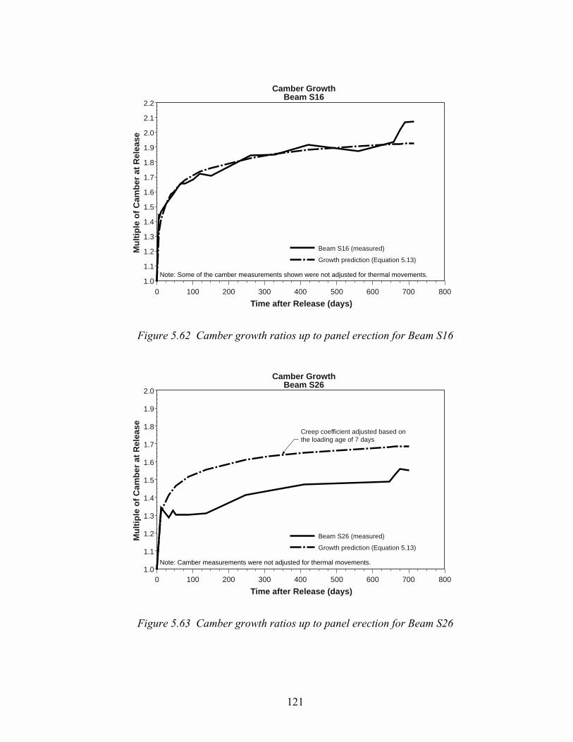
121
2.2
2.1
2.0
1.9
1.8
1.7
1.6
1.5
1.4
1.3
1.2
1.1
1.0
Mu
ltip
le o
f C
amb
er a
t R
elea
se
Time after Release (days)0 100 200 300 400 500 600 700 800
Beam S16 (measured)
Growth prediction (Equation 5.13)
Camber GrowthBeam S16
Note: Some of the camber measurements shown were not adjusted for thermal movements.
Figure 5.62 Camber growth ratios up to panel erection for Beam S16
2.0
1.9
1.8
1.7
1.6
1.5
1.4
1.3
1.2
1.1
1.0
Mu
ltip
le o
f C
amb
er a
t R
elea
se
Time after Release (days)0 100 200 300 400 500 600 700 800
Beam S26 (measured)
Growth prediction (Equation 5.13)
Camber GrowthBeam S26
Note: Camber measurements were not adjusted for thermal movements.
Creep coefficient adjusted based onthe loading age of 7 days
Figure 5.63 Camber growth ratios up to panel erection for Beam S26
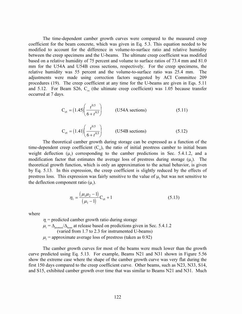
122
The time-dependent camber growth curves were compared to the measured creepcoefficient for the beam concrete, which was given in Eq. 5.3. This equation needed to bemodified to account for the difference in volume-to-surface ratio and relative humiditybetween the creep specimens and the U-beams. The ultimate creep coefficient was modifiedbased on a relative humidity of 75 percent and volume to surface ratios of 73.4 mm and 81.0mm for the U54A and U54B cross sections, respectively. For the creep specimens, therelative humidity was 55 percent and the volume-to-surface ratio was 25.4 mm. Theadjustments were made using correction factors suggested by ACI Committee 209procedures (19). The creep coefficient at any time for the U-beams are given in Eqs. 5.11and 5.12. For Beam S26, Ccu (the ultimate creep coefficient) was 1.05 because transferoccurred at 7 days.
� �� ���� �+��, � �$�(�� ������� � �
�
��
�
�
�
�
� �
� ��
�
�
� �� ���� �+��- � �$�(�� ������� � �
�
��
�
�
�
�
� �
� ��
�
�
The theoretical camber growth during storage can be expressed as a function of thetime-dependent creep coefficient (Cct), the ratio of initial prestress camber to initial beamweight deflection (�1) corresponding to the camber predictions in Sec. 5.4.1.2, and amodification factor that estimates the average loss of prestress during storage (�2). Thetheoretical growth function, which is only an approximation to the actual behavior, is givenby Eq. 5.13. In this expression, the creep coefficient is slightly reduced by the effects ofprestress loss. This expression was fairly sensitive to the value of �2 but was not sensitive tothe deflection component ratio (�1).
� �� �
�� �
�� �� �������
�
��� �
�
�
��
where�t = predicted camber growth ratio during storage�1 = prestress/beam at release based on predictions given in Sec. 5.4.1.2
(varied from 1.7 to 2.3 for instrumented U-beams)�2 = approximate average loss of prestress (taken as 0.92)
The camber growth curves for most of the beams were much lower than the growthcurve predicted using Eq. 5.13. For example, Beams N21 and N31 shown in Figure 5.56show the extreme case where the shape of the camber growth curve was very flat during thefirst 150 days compared to the creep coefficient curve. Other beams, such as N23, N33, S14,and S15, exhibited camber growth over time that was similar to Beams N21 and N31. Much

123
of the expected camber resulting from creep in the first 100 to 150 days was not achieved bythese beams and the growth thereafter was very small.
A few of the beams exhibited camber growth that agreed with the camber growthprediction based on Eq. 5.13. Beam S25, shown in Figure 5.59, had an erratic growth curvebut was close to the predicted creep curve for the 300-day period just before erection. At thetime of erection, Beam S25 was only 3 percent over the predicted camber growth ratio. Thecamber growth of Beams N22 and S16, shown in Figures 5.60 and 5.62, respectively, alsoshowed good agreement with the predicted growth curves.
Figures 5.56 to 5.59 show the camber growth curves for the companion beamsdiscussed in Sec. 5.4.1.1. Beam N32, shown in Figure 5.57, displayed growth that wasreasonably close to the predicted growth, while its companion beam (N33) displayed muchlower growth. The difference in camber throughout storage for Beams N32 and N33 wasmagnified when the camber growth ratio was used as a comparison. Both growth curvesshowed similar shapes, which was expected based on the camber response curves shown inFigure 5.52. Beams S14 and S15 exhibited camber growth ratios that were very closethroughout storage, while Beams S24 and S25 tended to separate at 200 days before erectionof the panels. Beams N21 and N31 also had very similar camber growth ratios duringstorage.
The camber growth ratio curves tended to exaggerate measured differences in camber,errors in the measuring systems, and analytical corrections because the quantities beingcompared were much smaller than the actual cambers. The general shape of each growthcurve was more important than examining differences between beams. However, the growthcurves shown for the beams in this study generally indicated that rate of camber growth in thefirst 100 to 200 days and the total camber resulting from creep were considerably less thanwhat was predicted with the camber growth equation shown in Eq. 5.13.
5.4.1.4 Comparison of Elastic Responses to Superimposed Loads
The measured deflections of the beams resulting from the deck panels and cast-in-place deck are shown in Table 5.10. The deflections of the interior beams were generallylarger than the deflections of the exterior beams because they carried a larger volume ofconcrete. The ratios of deflections of the interior beams and the exterior beam for each spanshould have been approximately equal to the ratio of concrete volumes carried by each beam.
The interior beams of spans two and three of the northbound bridge carried 30 and 27percent more deck panel load, respectively, than the exterior beam. The interior beams ofspans one and two of the southbound bridge carried 44 and 38 percent more load,respectively, than the exterior beam. The ratio of loading depended upon the average beamspacing for the particular span. The ratios of measured deflections for span three of thenorthbound bridge and span one of the southbound bridge were very close to the approximateratios of load carried. The ratios of measured deflections for the other spans were lower thanthe load ratios.
Similar ratios of measured deflections were expected after the cast-in-place deck waspoured on the beams. The overhangs on the exterior beams were not cast because future

124
plans called for widening each bridge. This meant that the load ratios resulting from the CIPdeck were nearly identical to the load ratios due the deck panels for all of the spans. The loadratios depended upon the actual deck thicknesses that were poured, which are shown in Sec.4.4.3. The measured deflections resulting from the CIP deck generally exhibited similarbehavior to the deflections caused by the deck panels.
Table 5.10 Summary of elastic responses resulting from superimposed loads for interiorand exterior beams
Measured Deflection (mm)Deck Panels2 Cast-in-Place Deck
Beam Group Interior1 Exterior Ratio3 Interior1 Exterior Ratio3
N21, N22, N23 32.8 27.7 1.18 36.7 29.7 1.24N31, N32, N33 32.4 24.9 1.30 33.7 26.7 1.26S14, S15, S16 29.9 19.8 1.51 26.8 24.1 1.11S24, S25, S26 37.1 32.5 1.14 41.1 32.1 1.28Notes:1.� Deflections represent an average of the two interior beams.2.� Measurements were not taken immediately after placement of the panels. There is a small
amount of time-dependent deflection in these values. Measurements also were notadjusted for thermal movements.
3.� Represents the ratio of deflection of interior beams to deflection of exterior beam.
The deflection ratios for the interior and exterior beams are much more complicatedthan simply the ratio of loads carried by the beams. Differences in span lengths andstiffnesses that existed among the beams affected the measured ratio of deflections. Also, thebeam spacings were not constant, which meant that the superimposed load varied linearlyalong the length of the beam. The relative deflections between beams varied with the ratio ofspan lengths raised to the fourth power. Therefore, small differences in span length had ameasurable effect on the deflection. As mentioned previously, the load ratios are goodapproximations of the expected deflection responses for the beams.
For the measured deflections resulting from the deck panels, corrections for thermalmovements were not made on camber readings both prior to and after placement. Also, thereading after placement was taken several days after the actual placement. Some smalladditional time-dependent deflection probably occurred in between those readings. Both ofthese circumstances contributed to the variation in the measured deflection ratios shown inTable 5.10.
5.4.2 Prestressing Strand Strain
The measured strain at the center of gravity of the prestressing strands (CGS) wasequivalent to the change in prestressing strand strain in the beams. The increase in themeasured compressive strain at the CGS represented the loss of prestress with time in the

125
beams, not including the loss resulting from relaxation of the strands after release.Comparisons of the measured initial CGS strains and the measured time-dependent CGSstrain responses were made for several of the instrumented beams. Additional comparisonswere made between the time-dependent strain responses and the measured creep andshrinkage strains obtained from the companion tests.
5.4.2.1 Measured and Predicted Concrete Strain at CGS at Release
The measured and predicted strains at CGS immediately after transfer of theprestressing force are summarized in Table 5.11. The predicted strains at release werecalculated assuming prestress losses of 2 percent resulting from relaxation and 2 percentresulting from shrinkage and strand temperature changes that occurred before transfer.Transformed section properties and the measured modulus of elasticity at release were usedfor the predictions as well.
Table 5.11 Measured and predicted compressive strain at midspan at CGS immediately aftertransfer
Beam SideMeasured CGS
Strain (���Predicted CGS
Strain (����Difference
(��� Ratio4
S141 E 875 573 302 1.53S152 W 582 566 16 1.03S152 E 588 566 22 1.04S162 W 613 594 19 1.03S161 E 552 594 -42 0.93S252 W 674 523 151 1.29S252 E 463 523 -60 0.89S262 W 727 603 124 1.21N211 W 677 642 35 1.05N211 E 731 642 89 1.14N221 E 454 545 -91 0.83N311 W 670 621 49 1.08N322 W 634 506 128 1.25N322 E 560 506 54 1.11N321 E 629 506 123 1.24
Notes:1.� These measurements were obtained from electrical resistance strain (ERSG) gages.2.� These measurements were obtained from vibrating wire (VW) gages.3.� Predicted strains at transfer were calculated using transformed section properties, 2 percent
loss for relaxation, 2 percent loss for temperature changes, and the measured elasticmodulus at release for the specific beam pour.
4.� Ratios were calculated as the measured strain divided by the predicted strain.

126
For many of the beams, the measured strains were within 10 percent of the predictedstrains. Several of the measured strains varied with the predicted strains by only 3 to 5percent. The strain measurements were generally higher than the predicted strains, whichcontradicted the low initial camber measurements that were observed for all of the beams.Based on the results found for initial camber, the measured strains were expected to be lowerthan the predictions, indicating a stiffer beam and/or an increase in the prestress losses beforerelease.
The post-release measurements were taken an average of one hour after transferbegan, so the possibility that creep and shrinkage had caused the strains to be higher waseliminated. The performances of the gages probably affected some of the measurements.However, the strains were consistently high for all of the beams and the errors between thepredicted and measured strains were fairly low for most of the beams. In addition, most ofthe gages remained stable for several days past release, as shown in Sec. 5.3.3.
Voids in the concrete around the vibrating wire gages also may have contributed tosome of the high strain measurements. The presence of voids would reduce the effectivemodulus of the concrete over the gage length. This would cause the strain readings to behigher than the actual strain at that section.
A more likely cause for the high measured strains at release may have been due touneven cooling through the depth of the beam prior to release. Hydration temperatures of upto 60 °C were observed in Beams S16 and N32 during casting. In addition, temperaturegradients as large as 9 °C between the top and bottom flanges were observed in these beams.Once the side forms were removed, these beams began to rapidly cool to a uniformtemperature. However, the prestressing bed probably offered some degree of restraint to thebeam as the beam began to shorten as a result of cooling and shrinkage. Evidence of thisrestraint was seen in the form of a regular pattern of cracks located at the stirrups andextending from the top of the beam to the lower part of the web.
The combination of uneven cooling and restraint of the bed may have caused anonlinear distribution of strain to develop in the beam. The tendency of the uneven coolingwas to induce a curvature in the beam, similar to the curvatures discussed in Sec. 5.3.1.However, if the bed were offering restraint at the bottom of the beam, that curvature wouldnot be fully developed. The strain distribution in the beam was most likely linear down tothe bottom flange, where the distribution became highly nonlinear owing to the restraint.
The strains that developed in the beams from uneven shortening prior to releaseprobably affected the strain measurements just after release. The baseline measurement forthe strain gages was taken immediately before transfer, when the effects of restraint werepresent in the beam. Upon transfer of the prestressing force, the restraint offered by the bedwas removed, allowing the thermal curvature induced by uneven cooling of the section tofully develop.
The release of restraint at the bottom flange would be evident in the strainmeasurements at the CGS after release. The CGS strain gage would be measuring the netcompressive strain resulting from the prestressing force and beam weight and an additionalcompressive strain that occurred once the restraint was removed and the thermal curvaturewas allowed to develop.
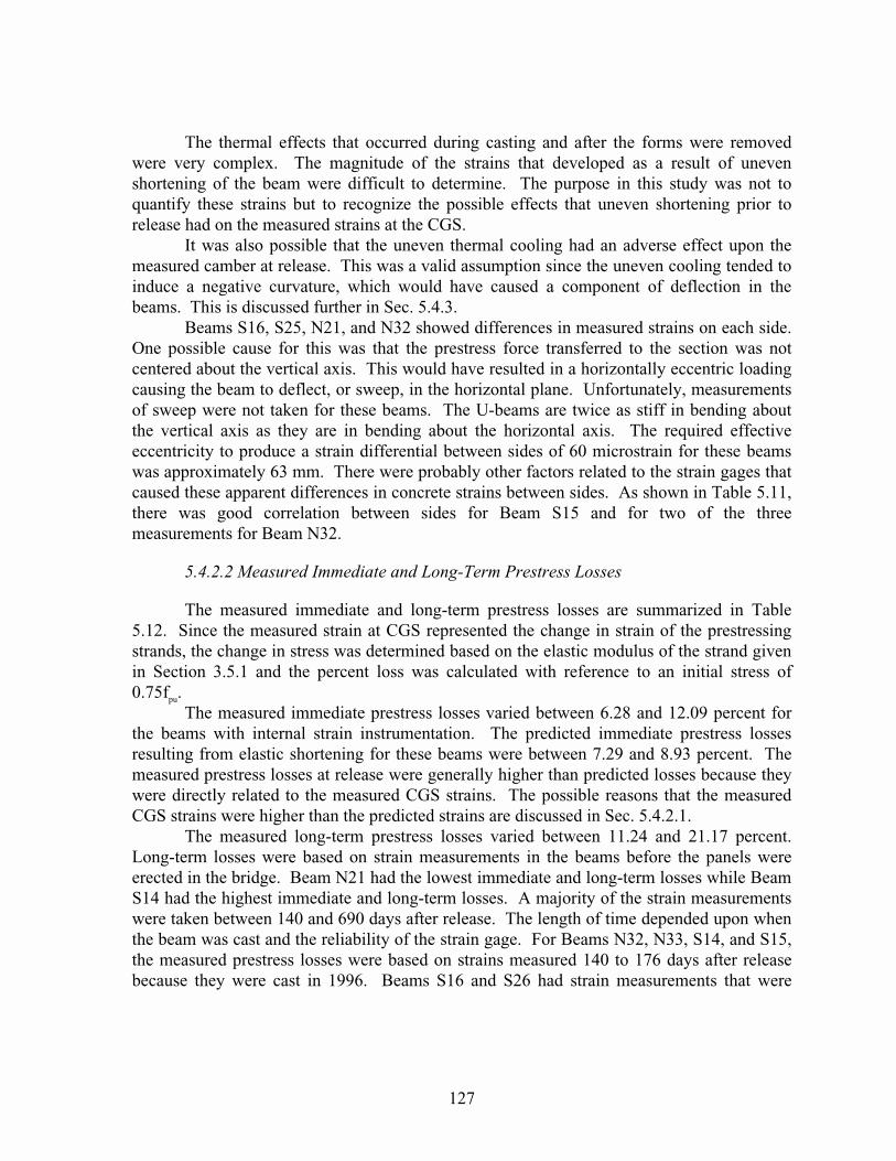
127
The thermal effects that occurred during casting and after the forms were removedwere very complex. The magnitude of the strains that developed as a result of unevenshortening of the beam were difficult to determine. The purpose in this study was not toquantify these strains but to recognize the possible effects that uneven shortening prior torelease had on the measured strains at the CGS.
It was also possible that the uneven thermal cooling had an adverse effect upon themeasured camber at release. This was a valid assumption since the uneven cooling tended toinduce a negative curvature, which would have caused a component of deflection in thebeams. This is discussed further in Sec. 5.4.3.
Beams S16, S25, N21, and N32 showed differences in measured strains on each side.One possible cause for this was that the prestress force transferred to the section was notcentered about the vertical axis. This would have resulted in a horizontally eccentric loadingcausing the beam to deflect, or sweep, in the horizontal plane. Unfortunately, measurementsof sweep were not taken for these beams. The U-beams are twice as stiff in bending aboutthe vertical axis as they are in bending about the horizontal axis. The required effectiveeccentricity to produce a strain differential between sides of 60 microstrain for these beamswas approximately 63 mm. There were probably other factors related to the strain gages thatcaused these apparent differences in concrete strains between sides. As shown in Table 5.11,there was good correlation between sides for Beam S15 and for two of the threemeasurements for Beam N32.
5.4.2.2 Measured Immediate and Long-Term Prestress Losses
The measured immediate and long-term prestress losses are summarized in Table5.12. Since the measured strain at CGS represented the change in strain of the prestressingstrands, the change in stress was determined based on the elastic modulus of the strand givenin Section 3.5.1 and the percent loss was calculated with reference to an initial stress of0.75fpu.
The measured immediate prestress losses varied between 6.28 and 12.09 percent forthe beams with internal strain instrumentation. The predicted immediate prestress lossesresulting from elastic shortening for these beams were between 7.29 and 8.93 percent. Themeasured prestress losses at release were generally higher than predicted losses because theywere directly related to the measured CGS strains. The possible reasons that the measuredCGS strains were higher than the predicted strains are discussed in Sec. 5.4.2.1.
The measured long-term prestress losses varied between 11.24 and 21.17 percent.Long-term losses were based on strain measurements in the beams before the panels wereerected in the bridge. Beam N21 had the lowest immediate and long-term losses while BeamS14 had the highest immediate and long-term losses. A majority of the strain measurementswere taken between 140 and 690 days after release. The length of time depended upon whenthe beam was cast and the reliability of the strain gage. For Beams N32, N33, S14, and S15,the measured prestress losses were based on strains measured 140 to 176 days after releasebecause they were cast in 1996. Beams S16 and S26 had strain measurements that were
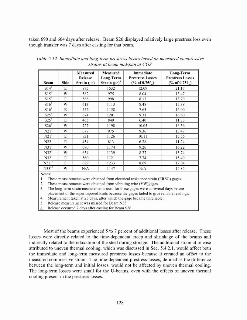
128
taken 690 and 664 days after release. Beam S26 displayed relatively large prestress loss eventhough transfer was 7 days after casting for that beam.
Table 5.12 Immediate and long-term prestress losses based on measured compressivestrains at beam midspan at CGS
Beam Side
MeasuredRelease
Strain (���
MeasuredLong-TermStrain (����
ImmediatePrestress Losses
(% of 0.75fpu)
Long-TermPrestress Losses
(% of 0.75fpu)S141 E 875 1532 12.09 21.17S152 W 582 975 8.04 13.47S152 E 588 998 8.13 13.79S162 W 613 1113 8.48 15.38S161 E 552 1158 7.63 16.00S252 W 674 1201 9.31 16.60S252 E 463 849 6.40 11.73S262 W 727 1198 10.05 16.56N211 W 677 975 9.36 13.47N211 E 731 1126 10.11 15.56N221 E 454 813 6.28 11.24N311 W 670 1174 9.26 16.22N322 W 634 1139 8.77 15.74N322 E 560 1121 7.74 15.49N321,4 E 629 1233 8.69 17.04N332,5 W N/A 1147 N/A 15.85
Notes:1.� These measurements were obtained from electrical resistance strain (ERSG) gages.2.� These measurements were obtained from vibrating wire (VW)gages.3.� The long-term strain measurements used for these gages were at several days before
placement of the superimposed loads because the gages failed to give reliable readings.4.� Measurement taken at 25 days, after which the gage became unreliable.5.� Release measurement was missed for Beam N33.6.� Release occurred 7 days after casting for Beam S26
Most of the beams experienced 5 to 7 percent of additional losses after release. Theselosses were directly related to the time-dependent creep and shrinkage of the beams andindirectly related to the relaxation of the steel during storage. The additional strain at releaseattributed to uneven thermal cooling, which was discussed in Sec. 5.4.2.1, would affect boththe immediate and long-term measured prestress losses because it created an offset to themeasured compressive strain. The time-dependent prestress losses, defined as the differencebetween the long-term and initial losses, would not be affected by uneven thermal cooling.The long-term losses were small for the U-beams, even with the effects of uneven thermalcooling present in the prestress losses.

129
5.4.2.3 Growth of Compressive Strain at CGS During Storage
Figures 5.64 to 5.69 show the time-dependent growth of compressive strain at CGS asplots of the time-varying multiple of the measured strain at release. These plots weredeveloped using the time-dependent strain responses for the beams, which are presented inSec. 5.3.3. Multiples of the compressive strain at release were calculated for several beamsup to a time approximately equal to the time of panel erection.
The time-dependent strain growth curves were compared to the predicted straingrowth curves based on the measured creep and shrinkage data for the companion specimens.The modified time-dependent creep coefficients for the U54A and U54B sections are givenby Eqs. 5.11 and 5.12. The ultimate shrinkage coefficient , shown in Eq. 5.6, was modifiedusing correction factors suggested by ACI Committee 209 procedures (19). The relativehumidities and volume-to-surface ratios used to calculate corrections are given in Sec.5.4.1.3. Equations 5.14 and 5.15 were used to calculate shrinkage strain for the U-beams. Theultimate shrinkage strain for Beam S26 was 224 microstrain to account for 7 days of steamcuring.
� � � �� �� �
���
���
�
� � �+��, � �$�(�� �������
�
�
��
�
��������
� � � �� �� �
���
���
�
� � �+��- � �$�(�� �������
�
�
��
�
��������
The theoretical growth of the compressive strain at the CGS during storage can beexpressed as a function of the time-dependent creep coefficient (Cct), the ratio of initialprestress strain to initial beam strain ( 1) corresponding to the strain predictions in Sec.5.4.2.1, a modification factor that estimates the average loss of prestress during storage ( 2),and the ratio of time-dependent shrinkage strain to initial strain owing to beam weight ( shr).The theoretical strain growth function, which is only an approximation to the actual behavior,is given by Eq. 5.16. In this expression, the creep coefficient is slightly reduced by theeffects of prestress loss. This expression was fairly sensitive to the values of 2 and shr butwas not sensitive to the strain component ratio ( 1).
� � � �� �
�� � �
��
� ��� ��
�������� �
��� �
�
�
��
where�t = predicted strain growth ratio during storage�1 = �prestress/�beam at release based on predictions given in Sec. 5.4.2.1
(varied from 3.7 to 4.0 for the beams shown in Figs. 5.64 to 5.69)�2 = approximate average loss of prestress (taken as 0.92)�shr = (�sh)t/�beam which is based on Eqs. 5.14 and 5.15 for shrinkage strain
and the predictions used to calculate release strain in Sec. 5.4.2.1
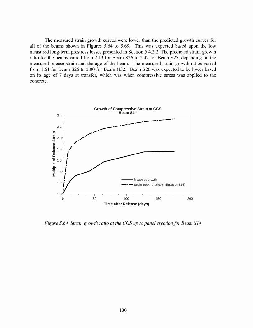
130
The measured strain growth curves were lower than the predicted growth curves forall of the beams shown in Figures 5.64 to 5.69. This was expected based upon the lowmeasured long-term prestress losses presented in Section 5.4.2.2. The predicted strain growthratio for the beams varied from 2.13 for Beam S26 to 2.47 for Beam S25, depending on themeasured release strain and the age of the beam. The measured strain growth ratios variedfrom 1.61 for Beam S26 to 2.00 for Beam N32. Beam S26 was expected to be lower basedon its age of 7 days at transfer, which was when compressive stress was applied to theconcrete.
2.4
2.2
2.0
1.8
1.6
1.4
1.2
1.0
Mu
ltip
le o
f R
elea
se S
trai
n
Time after Release (days)0 50 100 150 200
Measured growth
Strain growth prediction (Equation 5.16)
Growth of Compressive Strain at CGSBeam S14
Figure 5.64 Strain growth ratio at the CGS up to panel erection for Beam S14

131
2.4
2.2
2.0
1.8
1.6
1.4
1.2
1.0
Mu
ltip
le o
f R
elea
se S
trai
n
Time after Release (days)0 50 100 150 200
Measured growth (east midspan)
Measured growth (west midspan)
Strain growth prediction (Equation 5.16)
Growth of Compressive Strain at CGSBeam S15
Figure 5.65 Strain growth ratio at the CGS up to panel erection for Beam S15
2.6
2.4
2.2
2.0
1.8
1.6
1.4
1.2
1.0
Mu
ltip
le o
f R
elea
se S
trai
n
Time after Release (days)
0 100 200 300 400 500 600 700 800
Measured growth (west midspan)
Strain growth prediction (Equation 5.16)
Growth of Compressive Strain at CGSBeam S16
Figure 5.66 Strain growth ratio at the CGS up to panel erection for Beam S16

132
Measured growth (east midspan)
Measured growth (west midspan)
Strain growth prediction (Equation 5.16)
2.6
2.4
2.2
2.0
1.8
1.6
1.4
1.2
1.0
Mu
ltip
le o
f R
elea
se S
trai
n
Time after Release (days)0 100 200 300 400 500
Growth of Compressive Strain at CGSBeam S25
Figure 5.67 Strain growth ratio at the CGS up to panel erection for Beam S25
2.2
2.0
1.8
1.6
1.4
1.2
1.0
Mu
ltip
le o
f R
elea
se S
trai
n
Time after Release (days)
0 100 200 300 400 500 600 700 800
Measured growth (west midspan)
Strain growth prediction (Equation 5.16)
Growth of Compressive Strain at CGSBeam S26
Note: Release occurred 7 days after casing.
Strain growth prediction adjusted based onthe age of loading and additional steam curing.
Figure 5.68 Strain growth ratio at the CGS up to panel erection for Beam S26

133
Measured growth (east midspan)
Measured growth (west midspan)
Strain growth prediction (Equation 5.16)
2.4
2.2
2.0
1.8
1.6
1.4
1.2
1.0
Mu
ltip
le o
f R
elea
se S
trai
n
Time after Release (days)0 20 40 60 80 100 120 140 160
Growth of Compressive Strain at CGSBeam N32
Figure 5.69 Strain growth ratio at the CGS up to panel erection for Beam N32
For all of the beams, except the east side of Beam N32, the behavior of the measuredstrain growth curves was similar. During the initial 100 to 150 days of storage, significantlyless increase was observed in the measured growth curves than in the predicted curves.Much of the strain increase owing to creep and shrinkage during the first 100 days was notachieved by these beams and the growth thereafter was very small.
For Beam S15, shown in Figure 5.65, the strain growth curve was very flat during thefirst 150 days of storage compared to the predicted curve. Based on the strain growth curvefor Beam S15, one would expect the camber growth to be similar. Examination of Figure5.58 confirms that the camber growth curve for this beam had the same characteristics. BeamS15 had a strain growth ratio at CGS of 1.70 and a camber growth ratio of 1.63. The straingrowth ratio should be larger because of the component of compression owing to theprestressing force that does not cause curvature in the beam (P/A).
Not all of the beams had strain and camber growth characteristics that agreed as wellas was observed for Beam S15. Beams S16 and S25, shown in Figures 5.66 and 5.67respectively, exhibited strain growth ratios of approximately 1.83. These ratios were higherwhen compared to the other beams, but low compared to the predictions. Figures 5.59 and5.62 show the camber growth curves for Beams S25 and S16, respectively. The long-termcamber growth ratios for these beams were higher than the long-term strain growth ratios.Furthermore, the camber growth for both beams agreed with the prediction fairly well, whilethe strain growth did not.
The observance of low strain growth at CGS in the beams agreed with the observanceof low camber growth for most of the beams, as was shown in Sec. 5.4.1.3. With the

134
exception of Beams S16 and S25, the characteristics for the camber growth and strain growthcurves were similar. If the growth ratios for both sides of Beam N32 were averaged, then thestrain growth curve would show better agreement with the camber growth curve for BeamN32 shown in Figure 5.57.
Although it seemed that less creep and shrinkage were occurring in the beams duringstorage, the possible effects of uneven thermal cooling on the measured release strains wereevident in the strain growth ratios. If the release strains were artificially high owing to theeffects of uneven cooling, as discussed in Sec. 5.4.2.1, the strain growth ratios would belower. The strain growth ratio is defined as the measured strain at any time divided by themeasured strain at release. Since the measured strain was offset by the effects of unevencooling, the ratio would increase as the denominator, or measured release strain, decreased.However, even if the release strains were actually lower than what was measured, the time-dependent strain growth curves would still be significantly less than the predicted curves forall of the beams.
5.4.3 Midspan Strain Profiles at Release
The measured strain profiles at midspan at release represented the curvature in thebeam owing to the prestressing force and the weight of the beam. The measured midspancurvature could also be used as an indicator of the amount of camber in the beam at release.Comparisons of the measured and predicted midspan curvature at release for several of theinstrumented beams are presented in this section and are compared to the measured cambersat release and the measured strains at release.
The measured and predicted midspan curvatures at release are summarized in Table5.13. The measured midspan curvatures were determined by linear regression analysis. Thepredicted midspan curvatures were calculated based on the assumptions presented in Sec.5.4.1.2 for predicting midspan camber at release. The predicted curvatures at release werepositive because of the sign convention used in the calculations. A positive curvaturecorresponded to a moment that caused tension in the top fiber.
Differences between the measured and predicted midspan curvature varied from 1.21to -0.94 rad/mm (x10-7). A positive difference indicated that the measured curvature waslarger than the predicted curvature. The ratios of measured to predicted midspan curvaturesvaried from 0.62 for Beam S25 to 1.31 for Beam S14 and the average curvature ratio was0.95. Most of the measured curvature ratios agreed reasonably well with the predictedcurvatures. Five of the nine beams had at least one ratio of measured to predicted curvaturethat was between 0.94 and 1.02.
Wide variations in the measured curvatures were probably due to the use of threedifferent strain measuring systems to determine midspan curvatures. Generally the vibratingwire gages (VW) provided the most reliable data while the Demec surfaces strain gages werethe least reliable. The Demec surface strains were less accurate because there were nocorrections made for surface temperature differences between readings.
The measured curvature ratios at midspan are compared to the measured camber andCGS strain ratios in Table 5.14 for nine of the twelve instrumented beams. Whenever

135
possible, the data provided by the internal strain gages were used for the measuredcurvatures.
Table 5.13 Comparison of measured and predicted midspan curvatures at release
Beam
Source of
Data
Measured
Curvature1
(x10-7 rad/mm)
Predicted
Curvature2
(x10-7 rad/mm)
Difference
(x10-7 rad/mm) Ratio3
S14 ERSG(East) 5.15 3.94 1.21 1.31
S15 VW4 3.57 3.80 -0.23 0.94
S16 ERSG(East) 3.44 3.58 -0.14 0.96
S25 VW(East) 1.55 2.49 -0.94 0.62
S26 Demec4 3.59 3.52 0.07 1.02
N21 ERSG(West) 4.45 3.72 0.73 1.20
Demec4 2.85 3.72 -0.87 0.77
N22 Demec4 1.54 2.43 -0.89 0.63
N31 Demec4 3.40 3.61 -0.21 0.94
N32 VW(West) 3.17 2.80 0.37 1.13
ERSG(East) 2.70 2.80 -0.10 0.96
Notes:
1.� Measured curvatures were determined using a linear regression analysis of the data
2.� Predicted curvatures were based on the same assumptions used for predicting camber at
release, which are presented in Sec. 5.4.1.2.
3.� Values represent the ratio of measured to predicted curvatures
4.� Measured curvatures for each side were averaged after the linear regression analysis
The measured curvature ratios at release agreed with the measured camber ratios forfive of the nine beams shown in Table 5.14. The differences between the measured camberand curvature ratios for Beams S15, S25, S26, N22, and N31 were less than or equal to 0.06.For the remainder of the beams, the measured curvature ratios were significantly higher thanthe measured camber ratios.
The curvature ratios were lower than the strain ratios for seven of the nine beamsshown in Table 5.14. In addition, six of the nine beams had measured curvature ratios that
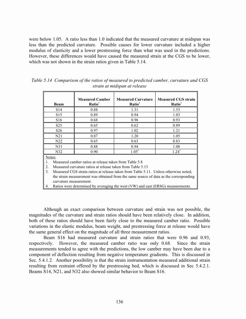
136
were below 1.05. A ratio less than 1.0 indicated that the measured curvature at midspan wasless than the predicted curvature. Possible causes for lower curvature included a highermodulus of elasticity and a lower prestressing force than what was used in the predictions.However, these differences would have caused the measured strain at the CGS to be lower,which was not shown in the strain ratios given in Table 5.14.
Table 5.14 Comparison of the ratios of measured to predicted camber, curvature and CGSstrain at midspan at release
BeamMeasured Camber
Ratio1Measured Curvature
Ratio2Measured CGS strain
Ratio3
S14 0.88 1.31 1.53S15 0.89 0.94 1.03S16 0.68 0.96 0.93S25 0.65 0.62 0.89S26 0.97 1.02 1.21N21 0.87 1.20 1.05N22 0.65 0.63 0.83N31 0.88 0.94 1.08N32 0.90 1.054 1.244
Notes:1.� Measured camber ratios at release taken from Table 5.82.� Measured curvature ratios at release taken from Table 5.133.� Measured CGS strain ratios at release taken from Table 5.11. Unless otherwise noted,
the strain measurement was obtained from the same source of data as the correspondingcurvature measurement.
4.� Ratios were determined by averaging the west (VW) and east (ERSG) measurements.
Although an exact comparison between curvature and strain was not possible, themagnitudes of the curvature and strain ratios should have been relatively close. In addition,both of these ratios should have been fairly close to the measured camber ratio. Possiblevariations in the elastic modulus, beam weight, and prestressing force at release would havethe same general effect on the magnitude of all three measurement ratios.
Beam S16 had measured curvature and strain ratios that were 0.96 and 0.93,respectively. However, the measured camber ratio was only 0.68. Since the strainmeasurements tended to agree with the predictions, the low camber may have been due to acomponent of deflection resulting from negative temperature gradients. This is discussed inSec. 5.4.1.2. Another possibility is that the strain instrumentation measured additional strainresulting from restraint offered by the prestressing bed, which is discussed in Sec 5.4.2.1.Beams S14, N21, and N32 also showed similar behavior to Beam S16.
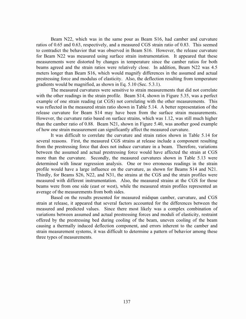
137
Beam N22, which was in the same pour as Beam S16, had camber and curvatureratios of 0.65 and 0.63, respectively, and a measured CGS strain ratio of 0.83. This seemedto contradict the behavior that was observed in Beam S16. However, the release curvaturefor Beam N22 was measured using surface strain instrumentation. It appeared that thesemeasurements were distorted by changes in temperature since the camber ratios for bothbeams agreed and the strain ratios were relatively close. In addition, Beam N22 was 4.5meters longer than Beam S16, which would magnify differences in the assumed and actualprestressing force and modulus of elasticity. Also, the deflection resulting from temperaturegradients would be magnified, as shown in Eq. 5.10 (Sec. 5.3.1).
The measured curvatures were sensitive to strain measurements that did not correlatewith the other readings in the strain profile. Beam S14, shown in Figure 5.35, was a perfectexample of one strain reading (at CGS) not correlating with the other measurements. Thiswas reflected in the measured strain ratio shown in Table 5.14. A better representation of therelease curvature for Beam S14 may have been from the surface strain measurements.However, the curvature ratio based on surface strains, which was 1.12, was still much higherthan the camber ratio of 0.88. Beam N21, shown in Figure 5.40, was another good exampleof how one strain measurement can significantly affect the measured curvature.
It was difficult to correlate the curvature and strain ratios shown in Table 5.14 forseveral reasons. First, the measured CGS strains at release include a component resultingfrom the prestressing force that does not induce curvature in a beam. Therefore, variationsbetween the assumed and actual prestressing force would have affected the strain at CGSmore than the curvature. Secondly, the measured curvatures shown in Table 5.13 weredetermined with linear regression analysis. One or two erroneous readings in the strainprofile would have a large influence on the curvature, as shown for Beams S14 and N21.Thirdly, for Beams S26, N22, and N31, the strains at the CGS and the strain profiles weremeasured with different instrumentation. Also, the measured strains at the CGS for thosebeams were from one side (east or west), while the measured strain profiles represented anaverage of the measurements from both sides.
Based on the results presented for measured midspan camber, curvature, and CGSstrain at release, it appeared that several factors accounted for the differences between themeasured and predicted values. Since there most likely was a complex combination ofvariations between assumed and actual prestressing forces and moduli of elasticity, restraintoffered by the prestressing bed during cooling of the beam, uneven cooling of the beamcausing a thermally induced deflection component, and errors inherent to the camber andstrain measurement systems, it was difficult to determine a pattern of behavior among thesethree types of measurements.

138
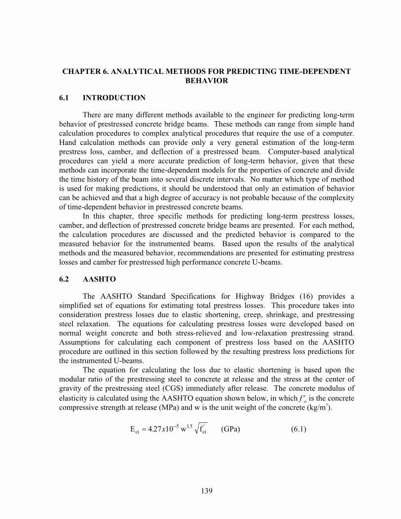
139
CHAPTER 6. ANALYTICAL METHODS FOR PREDICTING TIME-DEPENDENTBEHAVIOR
6.1 INTRODUCTION
There are many different methods available to the engineer for predicting long-termbehavior of prestressed concrete bridge beams. These methods can range from simple handcalculation procedures to complex analytical procedures that require the use of a computer.Hand calculation methods can provide only a very general estimation of the long-termprestress loss, camber, and deflection of a prestressed beam. Computer-based analyticalprocedures can yield a more accurate prediction of long-term behavior, given that thesemethods can incorporate the time-dependent models for the properties of concrete and dividethe time history of the beam into several discrete intervals. No matter which type of methodis used for making predictions, it should be understood that only an estimation of behaviorcan be achieved and that a high degree of accuracy is not probable because of the complexityof time-dependent behavior in prestressed concrete beams.
In this chapter, three specific methods for predicting long-term prestress losses,camber, and deflection of prestressed concrete bridge beams are presented. For each method,the calculation procedures are discussed and the predicted behavior is compared to themeasured behavior for the instrumented beams. Based upon the results of the analyticalmethods and the measured behavior, recommendations are presented for estimating prestresslosses and camber for prestressed high performance concrete U-beams.
6.2 AASHTO
The AASHTO Standard Specifications for Highway Bridges (16) provides asimplified set of equations for estimating total prestress losses. This procedure takes intoconsideration prestress losses due to elastic shortening, creep, shrinkage, and prestressingsteel relaxation. The equations for calculating prestress losses were developed based onnormal weight concrete and both stress-relieved and low-relaxation prestressing strand.Assumptions for calculating each component of prestress loss based on the AASHTOprocedure are outlined in this section followed by the resulting prestress loss predictions forthe instrumented U-beams.
The equation for calculating the loss due to elastic shortening is based upon themodular ratio of the prestressing steel to concrete at release and the stress at the center ofgravity of the prestressing steel (CGS) immediately after release. The concrete modulus ofelasticity is calculated using the AASHTO equation shown below, in which f�ci is the concretecompressive strength at release (MPa) and w is the unit weight of the concrete (kg/m3).
� � � ����
���� �� �� �
� �������������������������������������������
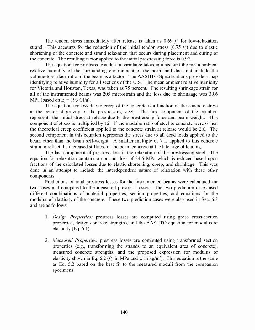
140
The tendon stress immediately after release is taken as 0.69 f�s for low-relaxationstrand. This accounts for the reduction of the initial tendon stress (0.75 f�s) due to elasticshortening of the concrete and strand relaxation that occurs during placement and curing ofthe concrete. The resulting factor applied to the initial prestressing force is 0.92.
The equation for prestress loss due to shrinkage takes into account the mean ambientrelative humidity of the surrounding environment of the beam and does not include thevolume-to-surface ratio of the beam as a factor. The AASHTO Specifications provide a mapidentifying relative humidity for all sections of the U.S. The mean ambient relative humidityfor Victoria and Houston, Texas, was taken as 75 percent. The resulting shrinkage strain forall of the instrumented beams was 205 microstrain and the loss due to shrinkage was 39.6MPa (based on Es = 193 GPa).
The equation for loss due to creep of the concrete is a function of the concrete stressat the center of gravity of the prestressing steel. The first component of the equationrepresents the initial stress at release due to the prestressing force and beam weight. Thiscomponent of stress is multiplied by 12. If the modular ratio of steel to concrete were 6 thenthe theoretical creep coefficient applied to the concrete strain at release would be 2.0. Thesecond component in this equation represents the stress due to all dead loads applied to thebeam other than the beam self-weight. A smaller multiple of 7 is applied to this concretestrain to reflect the increased stiffness of the beam concrete at the later age of loading.
The last component of prestress loss is the relaxation of the prestressing steel. Theequation for relaxation contains a constant loss of 34.5 MPa which is reduced based uponfractions of the calculated losses due to elastic shortening, creep, and shrinkage. This wasdone in an attempt to include the interdependent nature of relaxation with these othercomponents.
Predictions of total prestress losses for the instrumented beams were calculated fortwo cases and compared to the measured prestress losses. The two prediction cases useddifferent combinations of material properties, section properties, and equations for themodulus of elasticity of the concrete. These two prediction cases were also used in Sec. 6.3and are as follows:
1.� Design Properties: prestress losses are computed using gross cross-sectionproperties, design concrete strengths, and the AASHTO equation for modulus ofelasticity (Eq. 6.1).
�
2.� Measured Properties: prestress losses are computed using transformed sectionproperties (e.g., transforming the strands to an equivalent area of concrete),measured concrete strengths, and the proposed expression for modulus ofelasticity shown in Eq. 6.2 (f�ci in MPa and w in kg/m3). This equation is the sameas Eq. 5.2 based on the best fit to the measured moduli from the companionspecimens.

141
� �� � � ��
�� ���� � �
����
��� �����
������������������������������������������
��
The case using design properties represented the typical procedure for using theAASHTO Specifications to calculate prestress losses. The case using measured propertieswas chosen to examine the influence of transformed sections and the proposed equation forelastic modulus on total losses. These two prediction cases will be referred to asAASHTO(des.) and AASHTO(meas.) predictions.
The design and measured properties used for calculating prestress losses aresummarized in Tables 6.1 and 6.2, respectively. The transformed section properties used forcalculating prestress losses for the AASHTO(meas.) predictions are shown in Table 6.3. Thestrengths, moduli, and transformed section properties at 28 and 56 days were not used in theeither set of AASHTO predictions of prestress losses.
The span lengths and midspan moments used to calculate stresses at the CGS for bothcases are summarized in Table 6.4. The internal beam diaphragms were included in thecalculation of midspan moment due to the beam weight. The average measured deckthicknesses, which are given in Section 4.4.3, were used to calculate moments due to thecast-in-place deck for the case using measured properties. For both cases, the overhangs onthe exterior beams (S16, S26, N21, N31) were included in the moment calculations eventhough they actually were not cast with the deck. Exclusion of the overhangs would havecaused the creep loss to become excessively large for those beams. In determining themidspan moments due to the deck panel and CIP deck loads, a unit weight of 2403 kg/m3 wasassumed for the concrete.
The results of the AASHTO predicted total prestress losses are shown in Figures 6.1to 6.8. Predictions were made for the ten instrumented beams that had measured strains atthe center of gravity of the prestressing steel at midspan. The measured prestress losses weredetermined by calculating the product of the measured strain and the modulus of elasticity ofthe prestressing steel. For the pairs of companion beams (such as S14 and S15), the predictedlosses were nearly the same for each beam. Therefore, predicted losses for one of the twocompanion beams was used for comparison with the measured losses. The results for thecompanion beams are given in Figures 6.1 and 6.8.
The AASHTO(des.) predicted prestress losses varied between 26.18 and 34.11percent. The losses for Beams N21, N31, and S26 were the largest because they had thelargest products of initial prestressing force and eccentricity. As an example, the totalprestress loss for Beam S26 (shown in Figure 6.4) was comprised of 10.34 percent (144.4MPa) due to elastic shortening, 2.84 percent (39.6 MPa) due to shrinkage, 20.38 percent(284.6 MPa) due to creep, and 0.27 percent (3.8 MPa) due to relaxation. Beam S25, shownin Figure 6.3, had a slightly higher relaxation loss of 0.79 percent (11.0 MPa) but a lowerelastic shortening loss of 8.19 percent (114.4 MPa) and a lower creep loss of 14.42 percent(201.3 MPa). Both beams were U54B sections with similar span lengths. The differenceswere mainly due to Beam S26 having 19 more strands than Beam S25. Elastic shorteningand creep had the greatest effect on total losses for all of the beams.
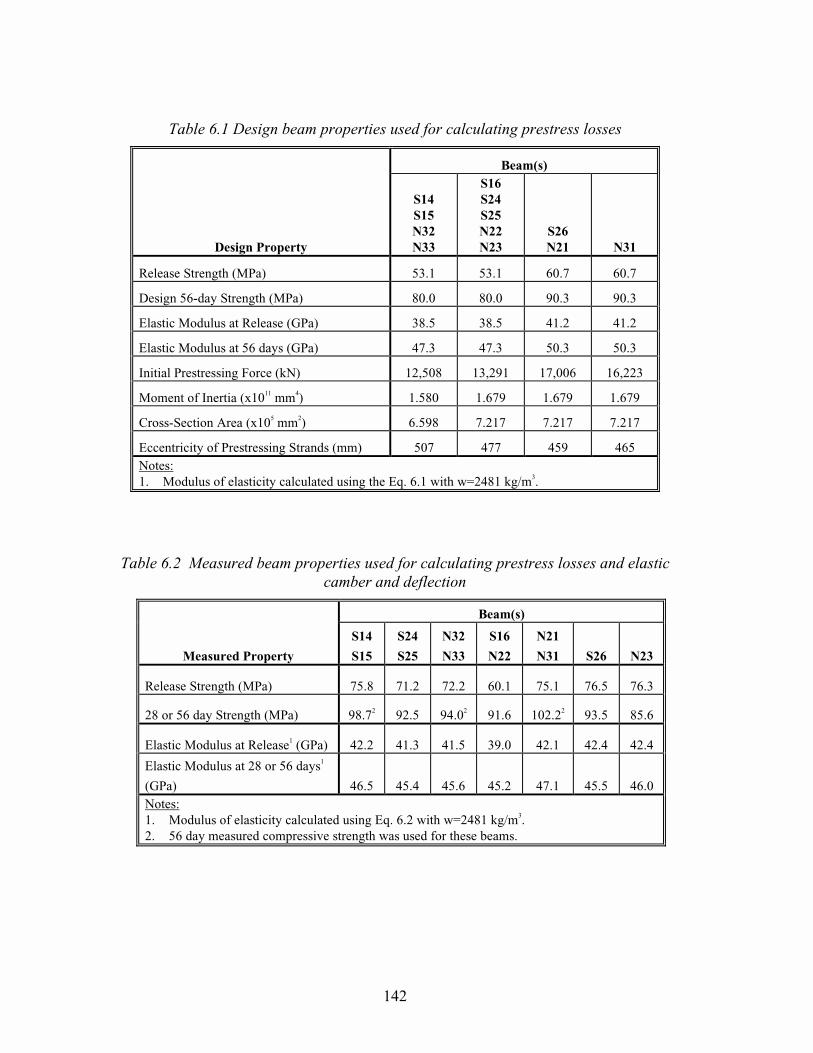
142
Table 6.1 Design beam properties used for calculating prestress losses
Beam(s)
Design Property
S14S15N32N33
S16S24S25N22N23
S26N21 N31
Release Strength (MPa) 53.1 53.1 60.7 60.7
Design 56-day Strength (MPa) 80.0 80.0 90.3 90.3
Elastic Modulus at Release (GPa) 38.5 38.5 41.2 41.2
Elastic Modulus at 56 days (GPa) 47.3 47.3 50.3 50.3
Initial Prestressing Force (kN) 12,508 13,291 17,006 16,223
Moment of Inertia (x1011 mm4) 1.580 1.679 1.679 1.679
Cross-Section Area (x105 mm2) 6.598 7.217 7.217 7.217
Eccentricity of Prestressing Strands (mm) 507 477 459 465Notes:1.� Modulus of elasticity calculated using the Eq. 6.1 with w=2481 kg/m3.
Table 6.2 Measured beam properties used for calculating prestress losses and elasticcamber and deflection
Beam(s)
Measured Property
S14
S15
S24
S25
N32
N33
S16
N22
N21
N31 S26 N23
Release Strength (MPa) 75.8 71.2 72.2 60.1 75.1 76.5 76.3
28 or 56 day Strength (MPa) 98.72 92.5 94.02 91.6 102.22 93.5 85.6
Elastic Modulus at Release1 (GPa) 42.2 41.3 41.5 39.0 42.1 42.4 42.4
Elastic Modulus at 28 or 56 days1
(GPa) 46.5 45.4 45.6 45.2 47.1 45.5 46.0Notes:1.� Modulus of elasticity calculated using Eq. 6.2 with w=2481 kg/m3.2.� 56 day measured compressive strength was used for these beams.

143
Table 6.3 Transformed section properties used for calculating prestress losses and elasticcamber and deflection
At Release At 28 or 56 days
Beam(s)
Area
(x105 mm2)
Moment of
Inertia
(x1011 mm4)
Eccentricity
(mm)
Moment of
Inertia
(x1011 mm4)
Eccentricity
(mm)
S14, S15 6.933 1.6617 483 1.6530 486
S16, N22 7.605 1.7638 453 1.7503 457
S24, S25 7.579 1.7582 455 1.7500 457
S26 7.662 1.7686 433 1.7613 435
N21 7.666 1.7693 433 1.7582 436
N23 7.568 1.7560 455 1.7488 457
N31 7.646 1.7675 439 1.7567 442
N32, N33 6.940 1.6633 483 1.6546 485
AASHTO Prestress Losses - Beams S14 and S15
35
30
25
20
15
10
5
0
Pre
stre
ss L
oss
(M
Pa)
450
400
350
300
250
200
150
100
50
0
Pre
stre
ss L
oss
(%
)
Measured long-term
Shrinkage
Creep
Relaxation
Elastic ShorteningAASHTOdesign
properties
AASHTOmeasuredproperties
Beam S14(Measured)
Beam S15(Measured)
Figure 6.1 AASHTO predicted prestress losses for Beams S14 and S15

144
AASHTO Prestress Losses - Beam S16
35
30
25
20
15
10
5
0
Pre
stre
ss L
oss
(M
Pa)
450
400
350
300
250
200
150
100
50
0
Pre
stre
ss L
oss
(%
)
Measured long-term
Shrinkage
Creep
Relaxation
Elastic ShorteningAASHTOdesign
properties
AASHTOmeasuredproperties
Beam S16(Measured)
Figure 6.2 AASHTO predicted prestress losses for Beam S16
AASHTO Prestress Losses - Beams S24 and S25
35
30
25
20
15
10
5
0
Pre
stre
ss L
oss
(M
Pa)
450
400
350
300
250
200
150
100
50
0
Pre
stre
ss L
oss
(%
)
Measured long-term
Shrinkage
Creep
Relaxation
Elastic ShorteningAASHTOdesign
properties
AASHTOmeasuredproperties
Beam S25(Measured)
Figure 6.3 AASHTO predicted prestress losses for Beams S24 and S25

145
AASHTO Prestress Losses - Beam S2640
35
30
25
20
15
10
5
0
Pre
stre
ss L
oss
(M
Pa)
550
500
450
400
350
300
250
200
150
100
50
0
Pre
stre
ss L
oss
(%
)Measured long-term
Shrinkage
Creep
Relaxation
Elastic ShorteningAASHTOdesign
properties
AASHTOmeasuredproperties
Beam S26(Measured)
Immediately afterCIP deck (beam
was 775 days old)
Figure 6.4 AASHTO predicted prestress losses for Beam S26
AASHTO Prestress Losses - Beam N2140
35
30
25
20
15
10
5
0
Pre
stre
ss L
oss
(M
Pa)
550
500
450
400
350
300
250
200
150
100
50
0
Pre
stre
ss L
oss
(%
)
Measured long-term
Shrinkage
Creep
Relaxation
Elastic ShorteningAASHTOdesign
properties
AASHTOmeasuredproperties
Beam N21(Measured)
395 daysin storage
Figure 6.5 AASHTO predicted prestress losses for Beam N21
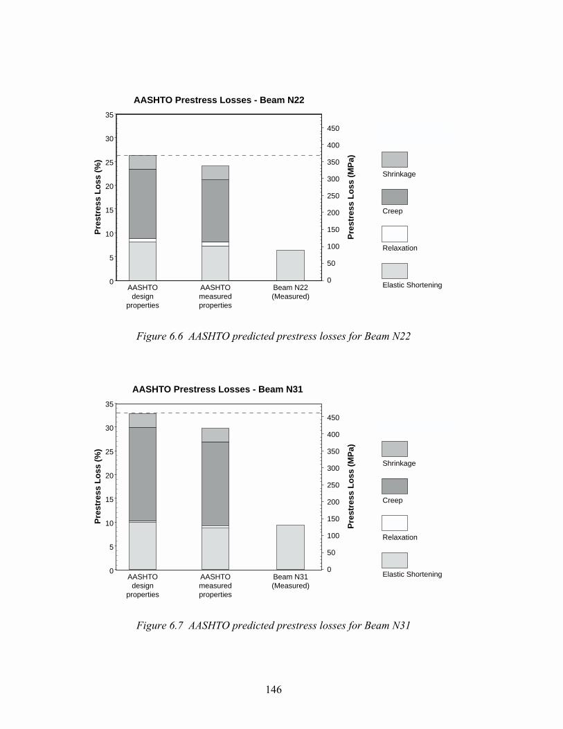
146
AASHTO Prestress Losses - Beam N22
35
30
25
20
15
10
5
0
Pre
stre
ss L
oss
(M
Pa)
450
400
350
300
250
200
150
100
50
0
Pre
stre
ss L
oss
(%
)
Measured long-term
Shrinkage
Creep
Relaxation
Elastic ShorteningAASHTOdesign
properties
AASHTOmeasuredproperties
Beam N22(Measured)
Figure 6.6 AASHTO predicted prestress losses for Beam N22
AASHTO Prestress Losses - Beam N31
35
30
25
20
15
10
5
0
Pre
stre
ss L
oss
(M
Pa)
450
400
350
300
250
200
150
100
50
0
Pre
stre
ss L
oss
(%
)
Measured long-term
Shrinkage
Creep
Relaxation
Elastic ShorteningAASHTOdesign
properties
AASHTOmeasuredproperties
Beam N31(Measured)
Figure 6.7 AASHTO predicted prestress losses for Beam N31

147
AASHTO Prestress Losses - Beams N32 and N33
35
30
25
20
15
10
5
0
Pre
stre
ss L
oss
(M
Pa)
450
400
350
300
250
200
150
100
50
0
Pre
stre
ss L
oss
(%
)
Measured long-term
Shrinkage
Creep
Relaxation
Elastic ShorteningAASHTOdesign
properties
AASHTOmeasuredproperties
Beam N32(Measured)
Beam N33(Measured)
221 daysin storage
Figure 6.8 AASHTO predicted prestress losses for Beams N32 and N33
Table 6.4 Midspan moments used to calculate prestress losses based on AASHTO and PCIprocedures
Midspan Moment (kN-m)
BeamSpan(m)
BeamWeight Panels
DesignCIP Deck
MeasuredCIP Deck
TotalDeck
(Design)Total Deck(Measured)
S14 35.55 2640 1514 1814 1922 3328 3436S15 36.01 2741 1533 1839 2058 3372 3591S16 36.49 3063 1098 2689 2846 3787 3944S24 39.83 3611 1633 1989 2339 3622 3972S25 40.33 3738 1651 2015 2369 3666 4020S26 40.84 3819 1237 3222 3487 4459 4724N21 40.90 3814 1140 3122 3203 4262 4343N22 41.07 3840 1493 1855 1962 3348 3455N23 41.25 3884 1499 1864 1971 3363 3470N31 40.35 3706 1067 2993 3069 4060 4136N32 40.50 3427 1366 1712 1810 3078 3176N33 40.66 3464 1370 1718 1816 3088 3186
Differences in the magnitude of creep loss were also a function of the span lengths ofthe beams. For Beams S14 and S15, shown in Figure 6.1, the loss due to elastic shortening

148
was 9.91 percent (138.3 MPa) and the loss due to creep was 18.39 percent (256.7 MPa). ForBeams N32 and N33, shown in Figure 6.8, the loss due to elastic shortening was 9.00 percent(125.7 MPa) and the loss due to creep was 16.62 percent (232.1 MPa). These beams were allU54A sections having 68 strands but Beams N32 and N33 had spans approximately fivemeters longer than the spans for Beams S14 and S15.
The large elastic shortening and creep losses for some of the beams caused the lossdue to strand relaxation to be underestimated. The form of the equation in the AASHTOSpecifications for calculating relaxation loss is not appropriate for high prestressing forcessuch as those applied to the U-beams. Despite this underestimation, the loss due to relaxationstill remains insignificant because of the use of low-relaxation strands.
The AASHTO(meas.) predicted prestress losses ranged from 23.46 to 30.78 percent.Examining Beam S26 (Figure 6.4) once again, the loss due to shrinkage remained the sameand the loss due to relaxation was nearly the same. However, the loss due to elasticshortening was reduced to 9.02 percent (125.9 MPa) and the loss due to creep was reduced to17.92 percent (250.2 MPa). This was a result of using transformed section properties, adifferent modulus of elasticity, and different deck moments.
Since the U-beams contained a large number of strands, using transformed sectionproperties resulted in a measurable increase in the area and moment of inertia of the sectionand a measurable decrease in the eccentricity of the strands for all beams. The differences insection properties can be observed by comparing Tables 6.1 and 6.3. As a result of usingtransformed section properties, the stress at the center of gravity of the strands at release waslower than the stress based on gross section properties. Consequently, the elastic shorteningand creep losses were lower.
The modulus of elasticity at release based on measured compressive strengths and Eq.6.2 was slightly higher that the design modulus of elasticity. This can be seen by examiningTables 6.1 and 6.2. The elastic moduli calculated with Eq. 6.2 were larger because themeasured release strengths were generally much higher than the design release strengths.Since the AASHTO equation (Eq. 6.1) did not overestimate the modulus of elasticity at thedesign release strengths, using the proposed equation with the higher measured strengthsyielded slightly higher values for elastic moduli. Figure 5.6 in Sec. 5.2.2 shows the graphs ofboth modulus of elasticity equations. As a result of the higher elastic moduli, the losses dueto elastic shortening were lower.
The measured deck thicknesses were larger than the design deck thickness for all ofthe beams. As a result, the midspan moments due to the deck panels and cast-in-place (CIP)deck were larger, as shown in Table 6.4. Consequently, the stress at the CGS was increasedwhich caused the loss due to creep to be less than the creep loss calculated using designproperties.
The measured prestress losses are compared to the AASHTO predicted prestresslosses in Figures 6.1 to 6.8. Measured losses varied between 10.56 and 17.38 percent. Thesevalues did not include the loss of prestress due to strand relaxation. Unless otherwiseindicated in the figures, measured long-term losses corresponded to a time approximatelyfive months after the CIP deck was completed. At that time, Beams S14, S15, and N32 wereapproximately 375 days old and Beams S16 and S25 were approximately 875 days old.

149
Based upon the measured strains after the completion of the deck, it appeared that long-termchanges in strain would be small.
As can be seen in Figures 6.1 to 6.5 and Figure 6.8, the measured long-term prestresslosses, which represented the effects of creep and shrinkage, were significantly less thaneither set of predicted long-term losses. The measured losses for Beams N21 and N33,shown in Figures 6.5 and 6.8, respectively, were significantly lower than predictions despitenot including the elastic gain in prestress and reduced creep loss that the deck panels and CIPdeck would have caused.
Comparisons of the measured and AASHTO predicted immediate losses due to elasticshortening are summarized in Figure 6.9. The ratios of measured to predicted elasticshortening losses are plotted for the instrumented beams shown in Figures 6.1 to 6.8. As canbe seen in Figure 6.9, the AASHTO(des.) predicted losses generally overestimated themeasured losses at release. The average ratio of measured losses to AASHTO(des.) predictedlosses was 0.96. If the results for Beam S14, which seemed to be abnormally high, wereremoved from the graph, the average ratio would become 0.92. The AASHTO(des.)predicted losses were higher because of the use of gross section properties and a low modulusof elasticity.
1.6
1.4
1.2
1.0
0.8
0.6
0.4
0.2
0.0
Mea
sure
d/P
red
icte
d
S14 S15 S16 S25 S26 N21 N22 N31 N32
vs. AASHTO (measured properties)
vs. AASHTO (design properties)
Measured vs. AASHTO Predicted Elastic Shortening
Figure 6.9 Summary of the ratios of measured to AASHTO predicted prestress losses atrelease
The AASHTO(meas.) predicted losses generally underestimated the measured lossesat release. The average ratio of measured losses to AASHTO(meas.) predicted losses was1.11. If the results for Beam S14 were removed from the graph, the average ratio would

150
become 1.07. The use of transformed section properties and a high modulus of elasticitycontributed to the predictions underestimating the measured values.
Comparisons of the measured and AASHTO predicted total losses are summarized inFigure 6.10. The differences between the predicted and measured total losses are plotted forthe instrumented beams shown in Figures 6.1 to 6.8. Unlike the comparisons of measuredand predicted elastic shortening losses shown in Figure 6.9, the differences betweenmeasured and predicted total losses were quite large. The graph shown in Figure 6.10represents the algebraic difference between the predicted total losses (in percent) using theAASHTO equations and the measured total losses (in percent) using the measured strains atCGS. AASHTO(des.) predicted losses and AASHTO(meas.) predicted losses overestimatedthe measured losses by an average of 16.5 and 13.4 percent, respectively. Differencesbetween the two prediction values were discussed earlier in this section.
25
20
15
10
5
0
Pre
dic
ted
- M
easu
red
(%
)
S14 S15 S16 S25 S26 N21 N32 N33
vs. AASHTO (measured properties)
vs. AASHTO (design properties)
Measured vs. AASHTO Predicted Long-Term Prestress Loss
Figure 6.10 Summary of the differences in measured and AASHTO predicted long-termprestress losses
Based on the summary shown in Figure 6.10, the AASHTO procedures grosslyoverestimated the long-term loss due to creep. It appeared that the equation for creep losswas not applicable for the high performance concrete U-beams. The theoretical creepcoefficient of 2.0 applied to the initial stress at CGS at release overestimated the actual creepcoefficient measured for the HPC beam mix, which is shown in Secs. 5.2.3 and 5.4.1.3. Thecreep and shrinkage tests on the HPC beam mix showed smaller strains than with normalstrength concrete, which indicated that less creep and shrinkage would occur in theinstrumented beams. In addition, the actual modular ratio at release for the HPC mix wasapproximately 5.0, meaning that the AASHTO creep coefficient applied to the strains at CGS

151
was 2.4 rather than 2.0. Also, the large stresses at the CGS, which were due to the largeprestressing forces and allowed for by very high concrete strength, contributed to the highcreep loss estimations.
6.3 PCI DESIGN HANDBOOK: PRESTRESS LOSSES, CAMBER, ANDDEFLECTION
6.3.1 Prestress Losses
The PCI Design Handbook (27) provides a simple method for estimating prestresslosses for prestressed concrete beams. The equations for losses due to elastic shortening,creep, shrinkage, and prestressing steel relaxation were adopted from the work of Zia et al.(38). This method is very similar to the AASHTO Specifications (16) procedure forcalculating prestress losses. In this section, the assumptions used in the PCI DesignHandbook method are reviewed and the predicted and measured prestress losses arepresented.
The equation for calculating the loss due to elastic shortening is the same as the onegiven in the AASHTO Specifications except that the reduction in the initial prestressing forceis 0.90 instead of 0.92. In addition, the PCI method suggests using 196.5 GPa for themodulus of elasticity of the strands. However, 193 GPa was used to remain consistent withthe other methods for predicting losses. The elastic moduli of the concrete were calculatedusing Eqs. 6.1 and 6.2.
The equation for prestress loss due to shrinkage considers the ambient relativehumidity and the volume-to-surface ratio of the beam cross-section. The ambient relativehumidity was assumed to be 75 percent, as in the AASHTO procedure. Since there were twoslightly different cross-sections for the instrumented U-beams, two shrinkage losses werecalculated. The ultimate shrinkage strains for the U54A and U54B beams were 169 and 166microstrain, respectively. The resulting prestress losses due to shrinkage for the U54A andU54B beams were 32.7 and 32.0 MPa, respectively.
The equation for prestress loss due to creep applies a creep coefficient of 2.0 to theinitial compressive strain at the CGS immediately after release and the tensile strain at theCGS due to superimposed dead loads. The 28-day modulus of elasticity is used forcalculating the modular ratio of prestressing steel to concrete. This attempts to account forthe age of the concrete when the superimposed dead load is placed on the beams. For someof the instrumented beams, the 56-day compressive strength was used for calculating themodulus of elasticity in the creep loss equation.
The equation for prestress loss due to relaxation of the strands is in the same form asthe AASHTO equation. A constant loss of 34.5 MPa is reduced by a fraction of the lossesdue to elastic shortening, creep, and shrinkage. However, the coefficient applied to theselosses is only 0.04. This means that the relaxation loss is less sensitive than the AASHTOequation to the magnitudes of the other losses.
Prestress loss estimations were calculated using the design and measured propertycases that are described in Sec. 6.2. The design and measured properties for the beams aresummarized in Tables 6.1 to 6.3. A summary of the midspan moments used to calculate

152
stresses at the center of gravity of the strands (CGS) is given in Table 6.4. These two caseswill be referred to as PCI(des.) and PCI(meas.) predicted prestress losses in this section.
The results of the PCI predicted total prestress losses are shown in Figures 6.11 to6.18. Predictions were made for the ten instrumented beams that had measured strains atCGS at midspan.
PCI Prestress Losses - Beams S14 and S15
30
25
20
15
10
5
0
Pre
stre
ss L
oss
(M
Pa)
400
350
300
250
200
150
100
50
0
Pre
stre
ss L
oss
(%
)
Measured long-term
Shrinkage
Creep
Relaxation
Elastic ShorteningPCIdesign
properties
PCImeasuredproperties
Beam S14(Measured)
Beam S15(Measured)
Figure 6.11 PCI predicted prestress losses for Beams S14 and S15
PCI Prestress Losses - Beam S1630
25
20
15
10
5
0
Pre
stre
ss L
oss
(M
Pa)
400
350
300
250
200
150
100
50
0
Pre
stre
ss L
oss
(%
)
Measured long-term
Shrinkage
Creep
Relaxation
Elastic ShorteningPCIdesign
properties
PCImeasuredproperties
Beam S16(Measured)
Figure 6.12 PCI predicted prestress losses for Beam S16

153
PCI Prestress Losses - Beams S24 and S2530
25
20
15
10
5
0
Pre
stre
ss L
oss
(M
Pa)
400
350
300
250
200
150
100
50
0
Pre
stre
ss L
oss
(%
)Measured long-term
Shrinkage
Creep
Relaxation
Elastic ShorteningPCIdesign
properties
PCImeasuredproperties
Beam S25(Measured)
Figure 6.13 PCI predicted prestress losses for Beams S24 and S25
PCI Prestress Losses - Beam S2630
25
20
15
10
5
0
Pre
stre
ss L
oss
(M
Pa)
400
350
300
250
200
150
100
50
0
Pre
stre
ss L
oss
(%
)
Measured long-term
Shrinkage
Creep
Relaxation
Elastic ShorteningPCIdesign
properties
PCImeasuredproperties
Beam S26(Measured)
Immediatelyafter
CIP deck
Figure 6.14 PCI predicted prestress losses for Beam S26
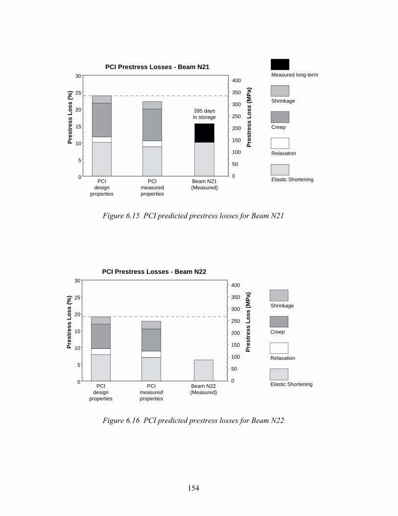
154
PCI Prestress Losses - Beam N2130
25
20
15
10
5
0
Pre
stre
ss L
oss
(M
Pa)
400
350
300
250
200
150
100
50
0
Pre
stre
ss L
oss
(%
)Measured long-term
Shrinkage
Creep
Relaxation
Elastic ShorteningPCIdesign
properties
PCImeasuredproperties
Beam N21(Measured)
395 daysin storage
Figure 6.15 PCI predicted prestress losses for Beam N21
PCI Prestress Losses - Beam N2230
25
20
15
10
5
0
Pre
stre
ss L
oss
(M
Pa)
400
350
300
250
200
150
100
50
0
Pre
stre
ss L
oss
(%
)
Measured long-term
Shrinkage
Creep
Relaxation
Elastic ShorteningPCIdesign
properties
PCImeasuredproperties
Beam N22(Measured)
Figure 6.16 PCI predicted prestress losses for Beam N22
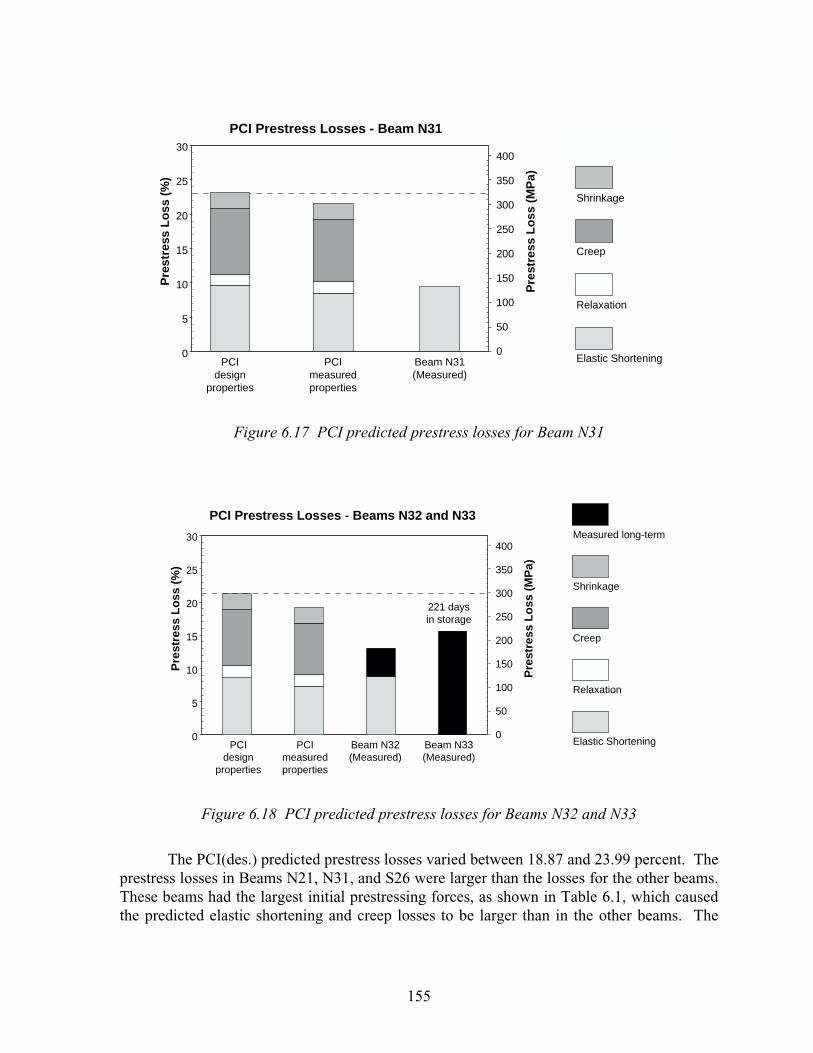
155
PCI Prestress Losses - Beam N3130
25
20
15
10
5
0
Pre
stre
ss L
oss
(M
Pa)
400
350
300
250
200
150
100
50
0
Pre
stre
ss L
oss
(%
)
Measured long-term
Shrinkage
Creep
Relaxation
Elastic ShorteningPCIdesign
properties
PCImeasuredproperties
Beam N31(Measured)
Figure 6.17 PCI predicted prestress losses for Beam N31
PCI Prestress Losses - Beams N32 and N33
30
25
20
15
10
5
0
Pre
stre
ss L
oss
(M
Pa)
400
350
300
250
200
150
100
50
0
Pre
stre
ss L
oss
(%
)
Measured long-term
Shrinkage
Creep
Relaxation
Elastic ShorteningPCIdesign
properties
PCImeasuredproperties
Beam N32(Measured)
Beam N33(Measured)
221 daysin storage
Figure 6.18 PCI predicted prestress losses for Beams N32 and N33
The PCI(des.) predicted prestress losses varied between 18.87 and 23.99 percent. Theprestress losses in Beams N21, N31, and S26 were larger than the losses for the other beams.These beams had the largest initial prestressing forces, as shown in Table 6.1, which causedthe predicted elastic shortening and creep losses to be larger than in the other beams. The
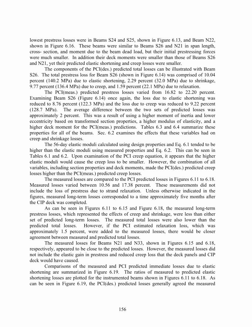
156
lowest prestress losses were in Beams S24 and S25, shown in Figure 6.13, and Beam N22,shown in Figure 6.16. These beams were similar to Beams S26 and N21 in span length,cross- section, and moment due to the beam dead load, but their initial prestressing forceswere much smaller. In addition their deck moments were smaller than those of Beams S26and N21, yet their predicted elastic shortening and creep losses were smaller.
The components of the PCI(des.) predicted total losses can be illustrated with BeamS26. The total prestress loss for Beam S26 (shown in Figure 6.14) was comprised of 10.04percent (140.2 MPa) due to elastic shortening, 2.29 percent (32.0 MPa) due to shrinkage,9.77 percent (136.4 MPa) due to creep, and 1.59 percent (22.1 MPa) due to relaxation.
The PCI(meas.) predicted prestress losses varied from 16.82 to 22.20 percent.Examining Beam S26 (Figure 6.14) once again, the loss due to elastic shortening wasreduced to 8.76 percent (122.3 MPa) and the loss due to creep was reduced to 9.22 percent(128.7 MPa). The average difference between the two sets of predicted losses wasapproximately 2 percent. This was a result of using a higher moment of inertia and lowereccentricity based on transformed section properties, a higher modulus of elasticity, and ahigher deck moment for the PCI(meas.) predictions. Tables 6.3 and 6.4 summarize theseproperties for all of the beams. Sec. 6.2 examines the effects that these variables had oncreep and shrinkage losses.
The 56-day elastic moduli calculated using design properties and Eq. 6.1 tended to behigher than the elastic moduli using measured properties and Eq. 6.2. This can be seen inTables 6.1 and 6.2. Upon examination of the PCI creep equation, it appears that the higherelastic moduli would cause the creep loss to be smaller. However, the combination of allvariables, including section properties and deck moments, made the PCI(des.) predicted creeplosses higher than the PCI(meas.) predicted creep losses.
The measured losses are compared to the PCI predicted losses in Figures 6.11 to 6.18.Measured losses varied between 10.56 and 17.38 percent. These measurements did notinclude the loss of prestress due to strand relaxation. Unless otherwise indicated in thefigures, measured long-term losses corresponded to a time approximately five months afterthe CIP deck was completed.
As can be seen in Figures 6.11 to 6.15 and Figure 6.18, the measured long-termprestress losses, which represented the effects of creep and shrinkage, were less than eitherset of predicted long-term losses. The measured total losses were also lower than thepredicted total losses. However, if the PCI estimated relaxation loss, which wasapproximately 1.5 percent, were added to the measured losses, there would be closeragreement between measured and predicted total losses.
The measured losses for Beams N21 and N33, shown in Figures 6.15 and 6.18,respectively, appeared to be close to the predicted losses. However, the measured losses didnot include the elastic gain in prestress and reduced creep loss that the deck panels and CIPdeck would have caused.
Comparisons of the measured and PCI predicted immediate losses due to elasticshortening are summarized in Figure 6.19. The ratios of measured to predicted elasticshortening losses are plotted for the instrumented beams shown in Figures 6.11 to 6.18. Ascan be seen in Figure 6.19, the PCI(des.) predicted losses generally agreed the measured

157
losses at release. The average ratio of measured losses to PCI(des.) predicted losses was0.99. If the results for Beam S14, which seemed to be abnormally high, were removed fromthe graph, that average ratio would become 0.95. The reduced factor of 0.9 applied to theinitial prestressing force caused this set of predictions to agree closely with themeasurements.
1.6
1.4
1.2
1.0
0.8
0.6
0.4
0.2
0.0
Mea
sure
d/P
red
icte
d
S14 S15 S16 S25 S26 N21 N22 N31 N32
vs. PCI (measured properties)
vs. PCI (design properties)
Measured vs. PCI Predicted Elastic Shortening
Figure 6.19 Summary of the ratios of measured to PCI predicted prestress losses due toelastic shortening
The PCI(meas.) predicted losses generally underestimated the measured losses atrelease. The average ratio of measured losses to PCI(meas.) predicted losses was 1.15. If theresults for Beam S14 were removed from the graph, that average ratio would become 1.10.In addition to the reduced factor of 0.90 applied to the initial prestressing force, the use oftransformed section properties and a high modulus of elasticity contributed to the predictionsunderestimating the measured values.
Comparisons of the measured and PCI predicted total losses are summarized inFigure 6.20. The differences between the predicted and measured total losses are plotted forthe instrumented beams shown in Figures 6.11 to 6.18. The differences between measuredand predicted total losses are large, although much less than what was found with theAASHTO predicted losses. The graph shown in Figure 6.20 represents the algebraicdifference between the predicted total losses (in percent) using the PCI equations and themeasured total losses (in percent) using the measured strains at the CGS. The PCI(des.) andPCI(meas.) predicted losses overestimated the measured losses by averages of 8.0 and 6.0percent, respectively. By adding relaxation to the measured losses, these differences would
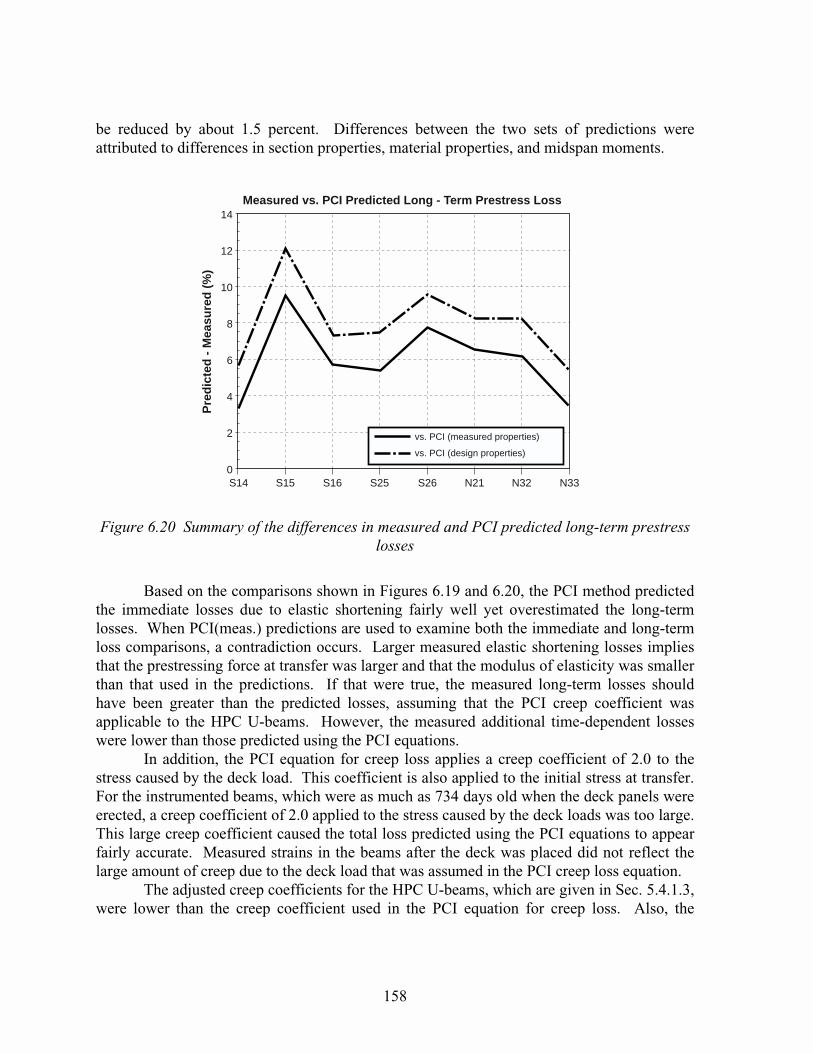
158
be reduced by about 1.5 percent. Differences between the two sets of predictions wereattributed to differences in section properties, material properties, and midspan moments.
14
12
10
8
6
4
2
0
Pre
dic
ted
- M
easu
red
(%
)
S14 S15 S16 S25 S26 N21 N32 N33
vs. PCI (measured properties)
vs. PCI (design properties)
Measured vs. PCI Predicted Long - Term Prestress Loss
Figure 6.20 Summary of the differences in measured and PCI predicted long-term prestresslosses
Based on the comparisons shown in Figures 6.19 and 6.20, the PCI method predictedthe immediate losses due to elastic shortening fairly well yet overestimated the long-termlosses. When PCI(meas.) predictions are used to examine both the immediate and long-termloss comparisons, a contradiction occurs. Larger measured elastic shortening losses impliesthat the prestressing force at transfer was larger and that the modulus of elasticity was smallerthan that used in the predictions. If that were true, the measured long-term losses shouldhave been greater than the predicted losses, assuming that the PCI creep coefficient wasapplicable to the HPC U-beams. However, the measured additional time-dependent losseswere lower than those predicted using the PCI equations.
In addition, the PCI equation for creep loss applies a creep coefficient of 2.0 to thestress caused by the deck load. This coefficient is also applied to the initial stress at transfer.For the instrumented beams, which were as much as 734 days old when the deck panels wereerected, a creep coefficient of 2.0 applied to the stress caused by the deck loads was too large.This large creep coefficient caused the total loss predicted using the PCI equations to appearfairly accurate. Measured strains in the beams after the deck was placed did not reflect thelarge amount of creep due to the deck load that was assumed in the PCI creep loss equation.
The adjusted creep coefficients for the HPC U-beams, which are given in Sec. 5.4.1.3,were lower than the creep coefficient used in the PCI equation for creep loss. Also, the

159
measured strains at release may have been artificially high due to the restraint effects of theprestressing bed which were discussed in Sec. 5.4.2.1. These two factors may explain whythe predicted elastic shortening losses were accurate while the predicted long-term losseswere much higher than the measured losses. In addition, the PCI equation for estimatingshrinkage strain underestimated the adjusted ultimate shrinkage strains for the HPC U-beamsby approximately 100 microstrain. However, this would result in an increase in the PCIshrinkage loss of only 1.4 percent (19.3 MPa).
6.3.2 Camber and Deflection
6.3.2.1 Elastic Camber and Deflection Due to Applied Loads
The PCI Design Handbook (27) provides equations for calculating elastic camber anddeflection responses that are based upon second moment-area principles. The expression formidspan camber due to the prestressing force is shown in Eq. 6.3. The prestressing force (P)used in this equation was taken as 0.90 multiplied by the initial prestressing force (Pi). Thisequation ignores strand debonding at the ends of the beams. If strand debonding wereincluded, it would cause the camber due to prestress to be an average of only 2 millimeterslower. The expression for the midspan deflection of a simply supported beam due to its owndistributed weight is shown in Eq. 6.4. The distributed load (w) was determined using a unitweight for the concrete of 2481 kg/m3. The deflection due to symmetrical internal diaphragmloads was calculated using Eq. 6.5. The total midspan deflection of the beam at release isshown in Eq. 6.6. The initial midspan camber at release is given in Eq. 6.7.
�� �������������������������������������������������������������������������
�� �
�
�
����� ��! ��������������������������������������������������������� ��
���� �
��
�
����"#�$! ����������������������������������������� �� ��
��
�
�
� �
�� �
�
�
�
�
�
�
�
��! ����� ��! ����"#�$!% ��������������������������������������������
#�&���� �� ��!� ��������������������������������������������������������
whereLs = design span length (m)a = length from centerline of bearing to the internal diaphragm (m)Pd = internal diaphragm load (kN)e = eccentricity of prestressing strands at midspan (mm)
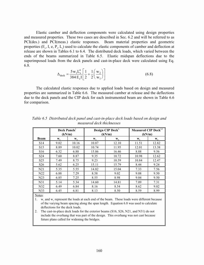
160
Elastic camber and deflection components were calculated using design propertiesand measured properties. These two cases are described in Sec. 6.2 and will be referred to asPCI(des.) and PCI(meas.) elastic responses. Beam material properties and geometricproperties (Ec, I, e, Pi, Ls) used to calculate the elastic components of camber and deflection atrelease are shown in Tables 6.1 to 6.4. The distributed deck loads, which varied between theends of the beams summarized in Table 6.5. Elastic midspan deflections due to thesuperimposed loads from the deck panels and cast-in-place deck were calculated using Eq.6.8.
���' ���������������������������������������������� ��
��
�
�
�
�
�
��
� �
���� �
�
�
�
�
� ��
�
�
The calculated elastic responses due to applied loads based on design and measuredproperties are summarized in Table 6.6. The measured camber at release and the deflectionsdue to the deck panels and the CIP deck for each instrumented beam are shown in Table 6.6for comparison.
Table 6.5 Distributed deck panel and cast-in-place deck loads based on design andmeasured deck thicknesses
Deck Panels1
(kN/m)Design CIP Deck1,
(kN/m)Measured CIP Deck1,2
(kN/m)Beam w1 w2 w1 w2 w1 w2
S14 9.02 10.16 10.87 12.10 11.51 12.82S15 8.89 10.02 10.74 11.95 12.01 13.38S16 6.32 6.88 15.86 16.46 8.88 9.56S24 7.60 8.87 9.35 10.72 10.98 12.62S25 7.49 8.75 9.23 10.59 10.84 12.47S26 5.62 6.25 15.11 15.79 8.44 9.24N21 5.35 5.55 14.82 15.04 7.33 7.56N22 6.88 7.29 8.58 9.02 9.08 9.50N23 6.85 7.25 8.55 8.98 9.04 9.50N31 5.14 5.34 14.60 14.81 7.09 7.31N32 6.49 6.84 8.16 8.54 8.62 9.02N33 6.45 6.81 8.13 8.50 8.59 8.99
Notes:1.� w1 and w2 represent the loads at each end of the beam. These loads were different because
of the varying beam spacing along the span length. Equation 6.8 was used to calculatedeflections for the deck loads.
2.� The cast-in-place deck loads for the exterior beams (S16, S26, N21, and N31) do notinclude the overhang that was part of the design. This overhang was not cast becausefuture plans called for widening the bridges.

161
Table 6.6 Comparison of PCI predicted and measured elastic responses to applied loads
Camber or Deflection (mm)Elastic
ComponentSource S14 S15 S16 S24 S25 S26 N21 N22 N23 N31 N32 N33
PCI (design) 147.6 151.5 146.3 174.3 178.8 211.4 211.9 185.4 187.0 199.2 191.7 193.2Camber due to
prestressPCI (meas) 122.4 125.6 131.2 148.4 152.1 184.3 185.9 166.2 155.7 175.4 161.3 162.6
PCI (design) 56.9 60.6 65.4 91.8 97.4 95.5 95.7 103.9 105.9 90.5 95.8 97.6Deflection due
to beam weightPCI (meas) 49.4 52.7 61.7 81.9 86.9 88.3 89.0 97.9 92.3 84.3 84.6 86.2
PCI (design) 90.7 90.9 80.9 82.5 81.4 115.9 116.2 81.5 81.1 108.7 95.9 95.6
PCI (meas) 73.0 72.9 69.5 66.5 65.2 96.0 96.9 68.3 63.4 91.1 76.7 76.4
Camber at
release
Measured 61.8 62.4 49.1 50.8 44.1 84.5 80.5 46.4 45.0 78.1 63.8 65.9
PCI (design) 26.6 27.7 19.1 33.9 35.2 25.4 23.5 33.0 33.4 21.4 31.2 31.5
PCI (meas) 26.0 27.0 19.2 34.0 35.2 26.8 24.0 33.2 33.0 21.9 30.9 31.3
Deflection due
to deck panels
Measured 29.7 30.0 19.8 36.0 38.1 32.5 27.7 32.2 33.3 24.9 32.0 32.7
PCI (design) 31.9 33.2 46.9 41.3 42.9 66.2 64.3 41.0 41.5 60.0 39.1 39.5
PCI (meas) 32.9 36.2 26.9 48.7 50.6 39.9 32.8 43.6 43.4 30.1 41.0 41.4
Deflection due
to CIP deck
Measured 24.9 28.7 24.1 41.4 40.7 32.1 29.5 38.1 35.3 26.7 35.3 32.0
The PCI(des.) calculated cambers at release varied from 80.9 mm (Beam S16) to116.2 mm (Beam N21). The largest release cambers were calculated for Beams N21, N31,and S26 because these beams had the most prestressing strands. The PCI(meas.) calculatedcambers at release varied between 63.4 mm (Beam N23) and 96.9 mm (Beam N21). Theinitial cambers calculated using measured properties were an average of 17.1 mm lowerbecause, for all of the beams, the modulus of elasticity and moment of inertia were higherand the eccentricity of the prestressing strands was lower than the design values. Clearly, theuse of measured properties had a significant effect on the prediction of camber at release.
The PCI(des.) calculated midspan deflections due to the deck panels varied between19.1 mm (Beam S16) and 35.2 mm (Beam S25). The PCI(meas.) calculated midspandeflections were nearly identical, varying between 19.2 mm and 35.2 mm. There appeared tobe no difference between the two cases because the changes in elastic modulus and momentof inertia tended to offset each other when measured properties were used rather than designproperties. Careful examination of Tables 6.1 to 6.3 shows this effect.
The PCI(des.) calculated midspan deflections due to the cast-in-place (CIP) deckvaried between 31.9 mm (Beam S14) and 66.2 mm (Beam S26). Large deflections werecalculate for Beams N21, N31, and S26 because these beams had long spans and carried theoverhang load. The PCI(meas.) calculated midspan deflections due to the CIP deck variedbetween 26.9 mm (Beam S16) and 50.6 mm (Beam S25). The deflections for all of theinterior beams were higher because the measured deck thicknesses were larger than thedesign thickness. As in the deck panel deflection calculations, the effect of a lower modulus
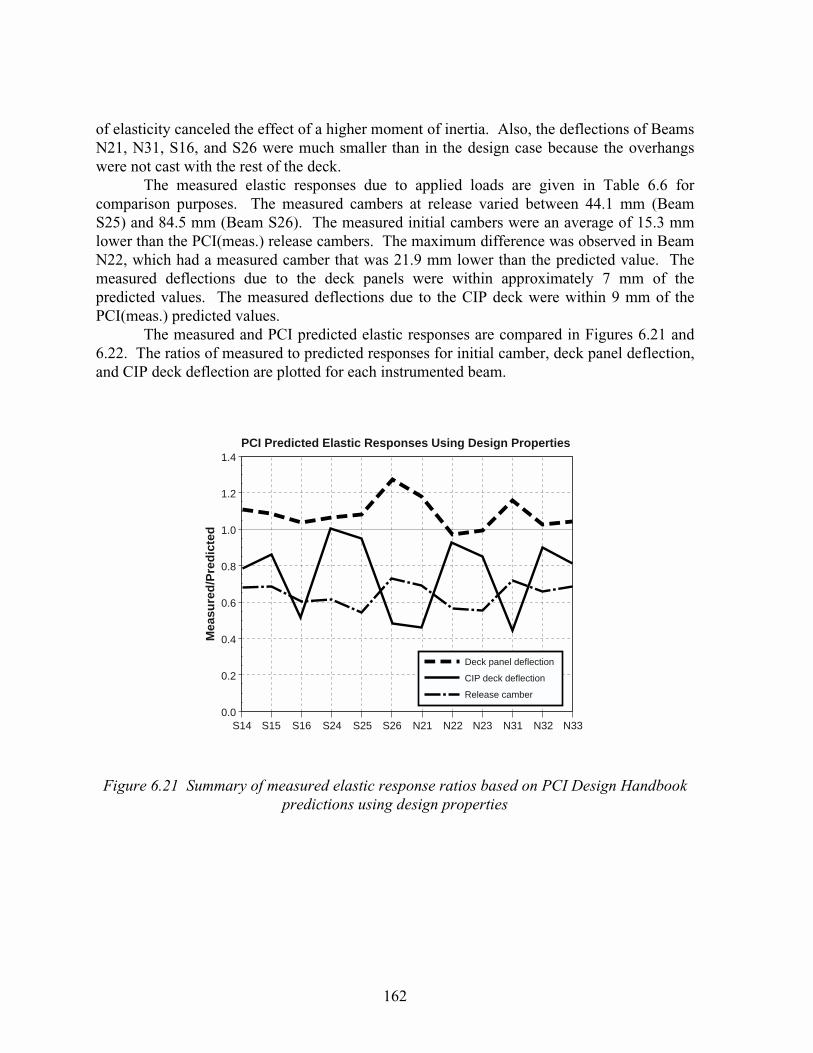
162
of elasticity canceled the effect of a higher moment of inertia. Also, the deflections of BeamsN21, N31, S16, and S26 were much smaller than in the design case because the overhangswere not cast with the rest of the deck.
The measured elastic responses due to applied loads are given in Table 6.6 forcomparison purposes. The measured cambers at release varied between 44.1 mm (BeamS25) and 84.5 mm (Beam S26). The measured initial cambers were an average of 15.3 mmlower than the PCI(meas.) release cambers. The maximum difference was observed in BeamN22, which had a measured camber that was 21.9 mm lower than the predicted value. Themeasured deflections due to the deck panels were within approximately 7 mm of thepredicted values. The measured deflections due to the CIP deck were within 9 mm of thePCI(meas.) predicted values.
The measured and PCI predicted elastic responses are compared in Figures 6.21 and6.22. The ratios of measured to predicted responses for initial camber, deck panel deflection,and CIP deck deflection are plotted for each instrumented beam.
1.4
1.2
1.0
0.8
0.6
0.4
0.2
0.0
Mea
sure
d/P
red
icte
d
S14 S15 S16 S24 S25 S26 N21 N22 N23 N31 N32 N33
Deck panel deflection
CIP deck deflection
Release camber
PCI Predicted Elastic Responses Using Design Properties
Figure 6.21 Summary of measured elastic response ratios based on PCI Design Handbookpredictions using design properties
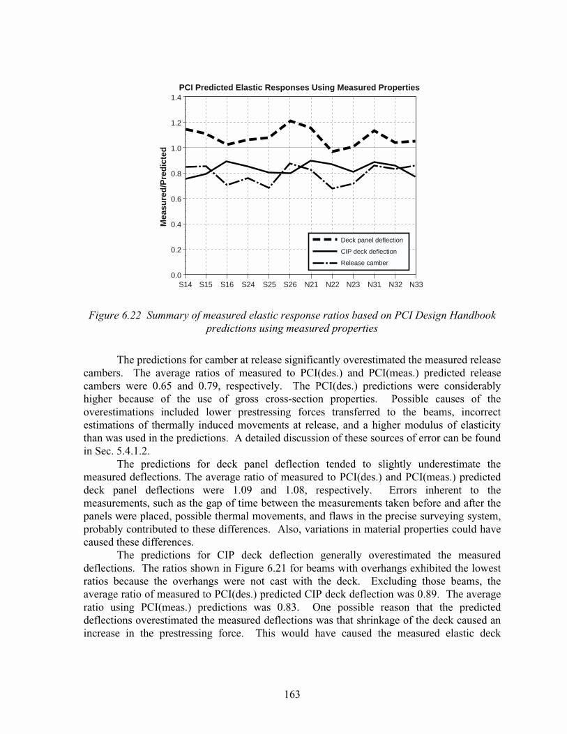
163
1.4
1.2
1.0
0.8
0.6
0.4
0.2
0.0
Mea
sure
d/P
red
icte
d
S14 S15 S16 S24 S25 S26 N21 N22 N23 N31 N32 N33
Deck panel deflection
CIP deck deflection
Release camber
PCI Predicted Elastic Responses Using Measured Properties
Figure 6.22 Summary of measured elastic response ratios based on PCI Design Handbookpredictions using measured properties
The predictions for camber at release significantly overestimated the measured releasecambers. The average ratios of measured to PCI(des.) and PCI(meas.) predicted releasecambers were 0.65 and 0.79, respectively. The PCI(des.) predictions were considerablyhigher because of the use of gross cross-section properties. Possible causes of theoverestimations included lower prestressing forces transferred to the beams, incorrectestimations of thermally induced movements at release, and a higher modulus of elasticitythan was used in the predictions. A detailed discussion of these sources of error can be foundin Sec. 5.4.1.2.
The predictions for deck panel deflection tended to slightly underestimate themeasured deflections. The average ratio of measured to PCI(des.) and PCI(meas.) predicteddeck panel deflections were 1.09 and 1.08, respectively. Errors inherent to themeasurements, such as the gap of time between the measurements taken before and after thepanels were placed, possible thermal movements, and flaws in the precise surveying system,probably contributed to these differences. Also, variations in material properties could havecaused these differences.
The predictions for CIP deck deflection generally overestimated the measureddeflections. The ratios shown in Figure 6.21 for beams with overhangs exhibited the lowestratios because the overhangs were not cast with the deck. Excluding those beams, theaverage ratio of measured to PCI(des.) predicted CIP deck deflection was 0.89. The averageratio using PCI(meas.) predictions was 0.83. One possible reason that the predicteddeflections overestimated the measured deflections was that shrinkage of the deck caused anincrease in the prestressing force. This would have caused the measured elastic deck
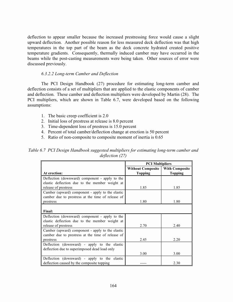
164
deflection to appear smaller because the increased prestressing force would cause a slightupward deflection. Another possible reason for less measured deck deflection was that hightemperatures in the top part of the beam as the deck concrete hydrated created positivetemperature gradients. Consequently, thermally induced camber may have occurred in thebeams while the post-casting measurements were being taken. Other sources of error werediscussed previously.
6.3.2.2 Long-term Camber and Deflection
The PCI Design Handbook (27) procedure for estimating long-term camber anddeflection consists of a set of multipliers that are applied to the elastic components of camberand deflection. These camber and deflection multipliers were developed by Martin (28). ThePCI multipliers, which are shown in Table 6.7, were developed based on the followingassumptions:
1.� The basic creep coefficient is 2.02.� Initial loss of prestress at release is 8.0 percent3.� Time-dependent loss of prestress is 15.0 percent4.� Percent of total camber/deflection change at erection is 50 percent5.� Ratio of non-composite to composite moment of inertia is 0.65
Table 6.7 PCI Design Handbook suggested multipliers for estimating long-term camber anddeflection (27)
PCI Multipliers
At erection:Without Composite
ToppingWith Composite
ToppingDeflection (downward) component - apply to theelastic deflection due to the member weight atrelease of prestress 1.85 1.85Camber (upward) component - apply to the elasticcamber due to prestress at the time of release ofprestress 1.80 1.80
Final:Deflection (downward) component - apply to theelastic deflection due to the member weight atrelease of prestress 2.70 2.40Camber (upward) component - apply to the elasticcamber due to prestress at the time of release ofprestress 2.45 2.20Deflection (downward) - apply to the elasticdeflection due to superimposed dead load only
3.00 3.00Deflection (downward) - apply to the elasticdeflection caused by the composite topping ----- 2.30
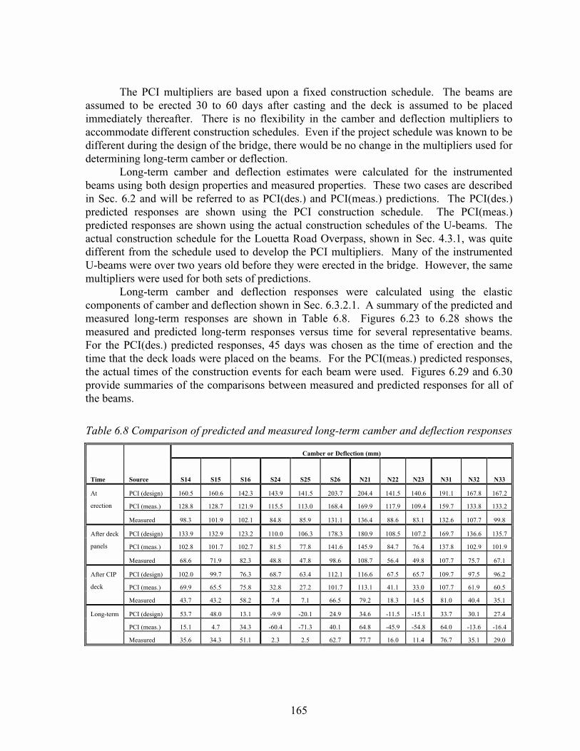
165
The PCI multipliers are based upon a fixed construction schedule. The beams areassumed to be erected 30 to 60 days after casting and the deck is assumed to be placedimmediately thereafter. There is no flexibility in the camber and deflection multipliers toaccommodate different construction schedules. Even if the project schedule was known to bedifferent during the design of the bridge, there would be no change in the multipliers used fordetermining long-term camber or deflection.
Long-term camber and deflection estimates were calculated for the instrumentedbeams using both design properties and measured properties. These two cases are describedin Sec. 6.2 and will be referred to as PCI(des.) and PCI(meas.) predictions. The PCI(des.)predicted responses are shown using the PCI construction schedule. The PCI(meas.)predicted responses are shown using the actual construction schedules of the U-beams. Theactual construction schedule for the Louetta Road Overpass, shown in Sec. 4.3.1, was quitedifferent from the schedule used to develop the PCI multipliers. Many of the instrumentedU-beams were over two years old before they were erected in the bridge. However, the samemultipliers were used for both sets of predictions.
Long-term camber and deflection responses were calculated using the elasticcomponents of camber and deflection shown in Sec. 6.3.2.1. A summary of the predicted andmeasured long-term responses are shown in Table 6.8. Figures 6.23 to 6.28 shows themeasured and predicted long-term responses versus time for several representative beams.For the PCI(des.) predicted responses, 45 days was chosen as the time of erection and thetime that the deck loads were placed on the beams. For the PCI(meas.) predicted responses,the actual times of the construction events for each beam were used. Figures 6.29 and 6.30provide summaries of the comparisons between measured and predicted responses for all ofthe beams.
Table 6.8 Comparison of predicted and measured long-term camber and deflection responses
Camber or Deflection (mm)
Time Source S14 S15 S16 S24 S25 S26 N21 N22 N23 N31 N32 N33
PCI (design) 160.5 160.6 142.3 143.9 141.5 203.7 204.4 141.5 140.6 191.1 167.8 167.2
PCI (meas.) 128.8 128.7 121.9 115.5 113.0 168.4 169.9 117.9 109.4 159.7 133.8 133.2
At
erection
Measured 98.3 101.9 102.1 84.8 85.9 131.1 136.4 88.6 83.1 132.6 107.7 99.8
PCI (design) 133.9 132.9 123.2 110.0 106.3 178.3 180.9 108.5 107.2 169.7 136.6 135.7
PCI (meas.) 102.8 101.7 102.7 81.5 77.8 141.6 145.9 84.7 76.4 137.8 102.9 101.9
After deck
panels
Measured 68.6 71.9 82.3 48.8 47.8 98.6 108.7 56.4 49.8 107.7 75.7 67.1
PCI (design) 102.0 99.7 76.3 68.7 63.4 112.1 116.6 67.5 65.7 109.7 97.5 96.2
PCI (meas.) 69.9 65.5 75.8 32.8 27.2 101.7 113.1 41.1 33.0 107.7 61.9 60.5
After CIP
deck
Measured 43.7 43.2 58.2 7.4 7.1 66.5 79.2 18.3 14.5 81.0 40.4 35.1
PCI (design) 53.7 48.0 13.1 -9.9 -20.1 24.9 34.6 -11.5 -15.1 33.7 30.1 27.4
PCI (meas.) 15.1 4.7 34.3 -60.4 -71.3 40.1 64.8 -45.9 -54.8 64.0 -13.6 -16.4
Long-term
Measured 35.6 34.3 51.1 2.3 2.5 62.7 77.7 16.0 11.4 76.7 35.1 29.0
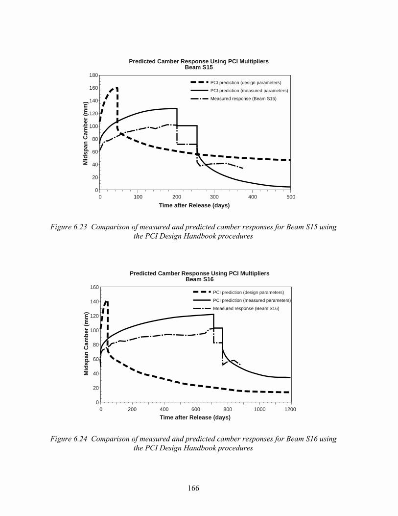
166
180
160
140
120
100
80
60
40
20
0
Mid
span
Cam
ber
(m
m)
0 100 200 300 400 500
PCI prediction (design parameters)
PCI prediction (measured parameters)
Measured response (Beam S15)
Predicted Camber Response Using PCI MultipliersBeam S15
Time after Release (days)
Figure 6.23 Comparison of measured and predicted camber responses for Beam S15 usingthe PCI Design Handbook procedures
160
140
120
100
80
60
40
20
0
Mid
span
Cam
ber
(m
m)
0 200 400 600 800 1000 1200
PCI prediction (design parameters)
PCI prediction (measured parameters)
Measured response (Beam S16)
Predicted Camber Response Using PCI MultipliersBeam S16
Time after Release (days)
Figure 6.24 Comparison of measured and predicted camber responses for Beam S16 usingthe PCI Design Handbook procedures

167
160
140
120
100
80
60
40
20
0
-20
-40
-60
-80
Mid
span
Cam
ber
(m
m)
0 200 400 600 800 1000 1200
PCI prediction (design parameters)
PCI prediction (measured parameters)
Measured response (Beam S25)
Predicted Camber Response Using PCI MultipliersBeam S25
Time after Release (days)
Figure 6.25 Comparison of measured and predicted camber responses for Beam S25 usingthe PCI Design Handbook procedures
220
200
180
160
140
120
100
80
60
40
20
0
Mid
span
Cam
ber
(m
m)
0 200 400 600 800 1000 1200
PCI prediction (design parameters)
PCI prediction (measured parameters)
Measured response (Beam N21)
Predicted Camber Response Using PCI MultipliersBeam N21
Time after Release (days)
Figure 6.26 Comparison of measured and predicted camber responses for Beam N21 usingthe PCI Design Handbook procedures
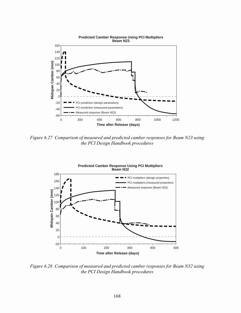
168
160
140
120
100
80
60
40
20
0
-20
-40
-60
Mid
span
Cam
ber
(m
m)
0 200 400 600 800 1000 1200
PCI prediction (design parameters)
PCI prediction (measured parameters)
Measured response (Beam N23)
Predicted Camber Response Using PCI MultipliersBeam N23
Time after Release (days)
Figure 6.27 Comparison of measured and predicted camber responses for Beam N23 usingthe PCI Design Handbook procedures
180
160
140
120
100
80
60
40
20
0
-20
Mid
span
Cam
ber
(m
m)
0 100 200 300 400 500
PCI multipliers (design properties)
PCI multipliers (measured properties)
Measured response (Beam N32)
Predicted Camber Response Using PCI MultipliersBeam N32
Time after Release (days)
Figure 6.28 Comparison of measured and predicted camber responses for Beam N32 usingthe PCI Design Handbook procedures
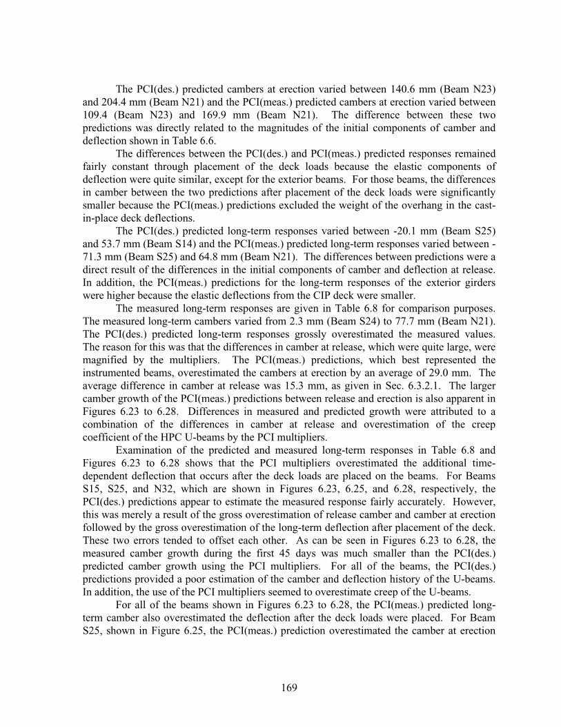
169
The PCI(des.) predicted cambers at erection varied between 140.6 mm (Beam N23)and 204.4 mm (Beam N21) and the PCI(meas.) predicted cambers at erection varied between109.4 (Beam N23) and 169.9 mm (Beam N21). The difference between these twopredictions was directly related to the magnitudes of the initial components of camber anddeflection shown in Table 6.6.
The differences between the PCI(des.) and PCI(meas.) predicted responses remainedfairly constant through placement of the deck loads because the elastic components ofdeflection were quite similar, except for the exterior beams. For those beams, the differencesin camber between the two predictions after placement of the deck loads were significantlysmaller because the PCI(meas.) predictions excluded the weight of the overhang in the cast-in-place deck deflections.
The PCI(des.) predicted long-term responses varied between -20.1 mm (Beam S25)and 53.7 mm (Beam S14) and the PCI(meas.) predicted long-term responses varied between -71.3 mm (Beam S25) and 64.8 mm (Beam N21). The differences between predictions were adirect result of the differences in the initial components of camber and deflection at release.In addition, the PCI(meas.) predictions for the long-term responses of the exterior girderswere higher because the elastic deflections from the CIP deck were smaller.
The measured long-term responses are given in Table 6.8 for comparison purposes.The measured long-term cambers varied from 2.3 mm (Beam S24) to 77.7 mm (Beam N21).The PCI(des.) predicted long-term responses grossly overestimated the measured values.The reason for this was that the differences in camber at release, which were quite large, weremagnified by the multipliers. The PCI(meas.) predictions, which best represented theinstrumented beams, overestimated the cambers at erection by an average of 29.0 mm. Theaverage difference in camber at release was 15.3 mm, as given in Sec. 6.3.2.1. The largercamber growth of the PCI(meas.) predictions between release and erection is also apparent inFigures 6.23 to 6.28. Differences in measured and predicted growth were attributed to acombination of the differences in camber at release and overestimation of the creepcoefficient of the HPC U-beams by the PCI multipliers.
Examination of the predicted and measured long-term responses in Table 6.8 andFigures 6.23 to 6.28 shows that the PCI multipliers overestimated the additional time-dependent deflection that occurs after the deck loads are placed on the beams. For BeamsS15, S25, and N32, which are shown in Figures 6.23, 6.25, and 6.28, respectively, thePCI(des.) predictions appear to estimate the measured response fairly accurately. However,this was merely a result of the gross overestimation of release camber and camber at erectionfollowed by the gross overestimation of the long-term deflection after placement of the deck.These two errors tended to offset each other. As can be seen in Figures 6.23 to 6.28, themeasured camber growth during the first 45 days was much smaller than the PCI(des.)predicted camber growth using the PCI multipliers. For all of the beams, the PCI(des.)predictions provided a poor estimation of the camber and deflection history of the U-beams.In addition, the use of the PCI multipliers seemed to overestimate creep of the U-beams.
For all of the beams shown in Figures 6.23 to 6.28, the PCI(meas.) predicted long-term camber also overestimated the deflection after the deck loads were placed. For BeamS25, shown in Figure 6.25, the PCI(meas.) prediction overestimated the camber at erection

170
by 27.1 mm and then significantly overestimated the long-term deflection after placement ofthe deck loads by 88.1 mm. Even though the elastic components of deflection werereasonably close, as discussed in Sec. 6.3.2.1, all of the instrumented beams displayed verylittle additional deflection after placement of the deck. This indicated that the multipliersapplied to the superimposed loads did not appropriately represent creep deflection of thecomposite HPC U-beam sections, especially when large differences between the actual andassumed construction schedule exist.
General trends that appeared between the PCI predicted and measured long-termcamber responses are presented in Figures 6.29 and 6.30. The differences between thepredicted and measured cambers at release, at erection, after the CIP deck was placed, andafter a long period of time are shown for both prediction cases. Positive differences indicatedthat the predicted values overestimated the measured values, while negative differencesindicated the opposite. The final measured camber values were considered long-term in thisstudy even though camber measurements will continue for several more years. The measuredloss of camber during the five month period after the CIP deck was cast indicated that verylittle change was occurring.
80
70
60
50
40
30
20
10
0
-10
-20
-30
-40
-50
Pre
dic
ted
- M
easu
red
(m
m)
S14 S15 S16 S24 S25 S26 N21 N22 N23 N31 N32 N33
At release
At erection
After CIP deck
End of service
PCI Predicted Camber Using Design Properties
Figure 6.29 Differences in measured and predicted long-term camber and deflection (basedon design parameters)
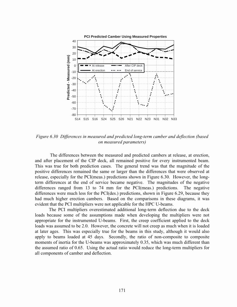
171
At release After CIP deck
At erection End of service
40
30
20
10
0
-10
-20
-30
-40
-50
-60
-70
-80
Pre
dic
ted
- M
easu
red
(m
m)
S14 S15 S16 S24 S25 S26 N21 N22 N23 N31 N32 N33
PCI Predicted Camber Using Measured Properties
Figure 6.30 Differences in measured and predicted long-term camber and deflection (basedon measured parameters)
The differences between the measured and predicted cambers at release, at erection,and after placement of the CIP deck, all remained positive for every instrumented beam.This was true for both prediction cases. The general trend was that the magnitude of thepositive differences remained the same or larger than the differences that were observed atrelease, especially for the PCI(meas.) predictions shown in Figure 6.30. However, the long-term differences at the end of service became negative. The magnitudes of the negativedifferences ranged from 13 to 74 mm for the PCI(meas.) predictions. The negativedifferences were much less for the PCI(des.) predictions, shown in Figure 6.29, because theyhad much higher erection cambers. Based on the comparisons in these diagrams, it wasevident that the PCI multipliers were not applicable for the HPC U-beams.
The PCI multipliers overestimated additional long-term deflection due to the deckloads because some of the assumptions made when developing the multipliers were notappropriate for the instrumented U-beams. First, the creep coefficient applied to the deckloads was assumed to be 2.0. However, the concrete will not creep as much when it is loadedat later ages. This was especially true for the beams in this study, although it would alsoapply to beams loaded at 45 days. Secondly, the ratio of non-composite to compositemoments of inertia for the U-beams was approximately 0.35, which was much different thanthe assumed ratio of 0.65. Using the actual ratio would reduce the long-term multipliers forall components of camber and deflection.

172
6.4 ANALYTICAL TIME-STEP METHOD
6.4.1 General
An analytical time-step method was developed based on the procedure outlined byBranson and Kripanarayanan (43). This method was developed on a computer spreadsheetprogram and used to predict the time-dependent prestress losses, camber, and deflection forall of the instrumented beams.
The time-dependent models for creep, shrinkage, and age-strength gain that weredeveloped from companion test data for the high performance concrete beam mix were usedin time-step method. These functions were assumed to be the most accurate representation ofthe properties of the instrumented beams.
The equations and assumptions used for the time-step analysis are presented in thefollowing sections. The resulting prestress loss and camber response predictions arepresented and compared to the measured behavior.
6.4.2 Prestress Losses
6.4.2.1 Analytical Procedure
The analytical procedure for calculating prestress losses involved calculating theinitial losses that occurred prior to release, the immediate loss during transfer of theprestressing force, the time-dependent losses due to creep, shrinkage, and relaxation overdiscrete time intervals, and instantaneous gains in prestress that occurred when the deckpanels and cast-in-place deck were placed on the beams. The effect of differential shrinkageof the deck was also considered. The total losses at any time were determined by summingthe instantaneous prestress losses (or gains) and the incremental losses that occurred duringthe previous time intervals.
The initial prestress losses that were assumed to occur between initial stressing of thestrands and release included losses due to increases in temperature of the strands, relaxation,and shrinkage after the side forms were stripped. The initial stress to which the strands werepulled was assumed to be 0.75fpu (1396 MPa). It was assumed that a 2 percent loss occurreddue to increased temperature of the strands, three days occurred between initial stressing andrelease, and 12 hours occurred between stripping the side forms and release. Equation 6.9,taken from the PCI Committee Report on Prestress Losses (56), was used to calculaterelaxation loss. Equation 6.10 was used to calculated shrinkage strain. The shrinkage losswas the product of the shrinkage strain and the modulus of elasticity of the prestressing steel,which was assumed to be 193 GPa.
(� �&)$ �
�
�
��� � ��
�� ��
�*
� ���
��
��
���
�
� �����������������������������������������
wheret = time after initial stressing (hours)fsi = initial stress in the strands (MPa)fpy = 0.1 percent offset yield strength taken as 0.9fpu (MPa)
173
� � � �� ��" � �" +
���
���
�
��
�
�
��
�
� ������������������������������������������������������
where(�sh)u = ultimate shrinkage strain adjusted for volume-to-surface ratio and
75 percent relative humidity (given in Table 6.9)t = time after stripping of the side forms (days)
Table 6.9 Ultimate creep and shrinkage coefficients for U-beams
U-beam Cross section Ultimate shrinkage coefficient (��� Ultimate creep coefficient (Ccu)
U54A 279 1.45
U54B 269 1.41
The immediate loss at transfer due to elastic shortening was calculated using thetransformed section properties, material properties calculated using Eqs. 6.11 and 6.12, beamloads based on a concrete unit weight of 2481 kg/m3 (including the diaphragms), design spanlengths shown in Table 6.4, and the actual time between casting and release, which are shownin Sec. 4.3.1. Equation 6.11 was developed in Sec. 5.2.1 based on data from member-curedspecimens. The elastic shortening loss was determined exactly using an iterative procedure.
� � � �� ,�
�� �% ��� ���
�
���
����� � ������-�������������������������������������������������
� �� ���� � �����
���� �
�
�� ��
�������
��� �
�����������������������������������������
The time-dependent losses were calculated over very short time intervals just afterrelease and then over larger time intervals as the changes in creep and shrinkage became less.Equation 6.13 was used to calculate the creep coefficient at any time.
� �. .�
� �� � �+
��
�� �
�
�
��
�
� �����������������������������������������������������������
whereCcu = ultimate creep coefficient adjusted for volume-to-surface ratio and
75 percent relative humidity (given in Table 6.9)t = time after release (days)
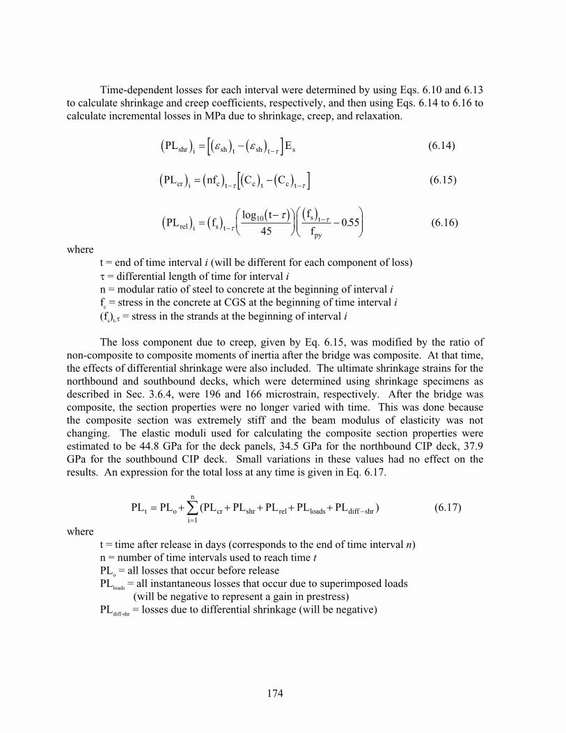
174
Time-dependent losses for each interval were determined by using Eqs. 6.10 and 6.13to calculate shrinkage and creep coefficients, respectively, and then using Eqs. 6.14 to 6.16 tocalculate incremental losses in MPa due to shrinkage, creep, and relaxation.
� � � � � �� ��� ��"# � �" � �" � �� ��
� ��
�����������������������������������������������������
� � � � � � � �� ��� /� . .�# � � � � � � �� �
� �� ������������������������������������������������ �
� � � �� � � �
�� �&)$ � �
��#�& � � �
� �
�*
���
��
�
� ��
���
�
��
��
����
� � ������������������������������
wheret = end of time interval i (will be different for each component of loss)� = differential length of time for interval in = modular ratio of steel to concrete at the beginning of interval ifc = stress in the concrete at CGS at the beginning of time interval i(fs)t-� = stress in the strands at the beginning of interval i
The loss component due to creep, given by Eq. 6.15, was modified by the ratio ofnon-composite to composite moments of inertia after the bridge was composite. At that time,the effects of differential shrinkage were also included. The ultimate shrinkage strains for thenorthbound and southbound decks, which were determined using shrinkage specimens asdescribed in Sec. 3.6.4, were 196 and 166 microstrain, respectively. After the bridge wascomposite, the section properties were no longer varied with time. This was done becausethe composite section was extremely stiff and the beam modulus of elasticity was notchanging. The elastic moduli used for calculating the composite section properties wereestimated to be 44.8 GPa for the deck panels, 34.5 GPa for the northbound CIP deck, 37.9GPa for the southbound CIP deck. Small variations in these values had no effect on theresults. An expression for the total loss at any time is given in Eq. 6.17.
�� �� ��� �� �� �� �� �� ) �# �"# #�& &)��� ���� �"#
� �
/
� � � � � � ��� �������������������������
wheret = time after release in days (corresponds to the end of time interval n)n = number of time intervals used to reach time tPLo = all losses that occur before releasePLloads = all instantaneous losses that occur due to superimposed loads
(will be negative to represent a gain in prestress)PLdiff-shr = losses due to differential shrinkage (will be negative)

175
Calculations for a typical time interval began by calculating concrete compressivestrength using Eq. 6.11, calculating the elastic modulus using Eq. 6.12, and then calculatingtransformed section properties. Incremental losses were calculated using Eqs. 6.14 to 6.16,summed, and added to the total prestress loss that was determined at the end of the previoustime interval. This operation can be represented by Eq. 6.17. Based on the new value forprestress loss, a new strand stress was determined. This strand stress was used for calculatingrelaxation and creep losses in the next time interval.
6.4.2.2 Predicted Prestress Losses
The measured and predicted prestress losses at the CGS at midspan using theanalytical time-step method are shown in Figures 6.31 to 6.38. Results were shown for thebeams that had measured strains at midspan at the CGS for a lengthy period of time. Asummary of the measured and predicted prestress losses at release, at erection, after the deckloads, and long-term are shown in Table 6.10.
Table 6.10 Summary of measured and predicted prestress losses using the analytical time-step method
Prestress Losses1,3 (%)
Time Source S14 S155 S16 S255 S26 N21 N22 N31 N32 N33
Elastic
Shortening
Time-step 8.09 8.00 7.40 6.89 8.22 8.83 6.80 8.51 7.36 ----
Measured 12.10 8.09 8.48 7.86 10.05 10.11 6.28 9.26 8.77 ----
At erection Time-step 22.32 22.15 22.69 20.83 21.50 24.024 ---- ---- 21.17 21.054
Measured 25.31 17.77 19.48 18.50 20.97 19.764 ---- ---- 19.88 19.814
After CIP deck Time-step 19.53 19.23 20.69 17.77 19.29 ---- ---- ---- 18.47 ----
Measured 21.88 15.11 17.68 15.98 18.81 ---- ---- ---- 17.50 ----
Long-term2 Time-step 19.57 19.31 20.66 17.75 ---- ---- ---- ---- 18.52 ----
Measured 21.51 14.68 17.17 15.44 ---- ---- ---- ---- 17.14 ----
Notes:
1.� Measured losses after release include approximately 4 percent for relaxation, shrinkage, and temperature effects that
were assumed to occur before release in the analytical time-step model.
2.� Long-term predictions correspond to the time of the last gage measurement.
3.� Measured losses do not include loss due to relaxation after release.
4.� Measurements were before erection because the gage stopped giving quality results.
5.� Measured losses were determined using an average of the measured strains on both sides of the beam at midspan.
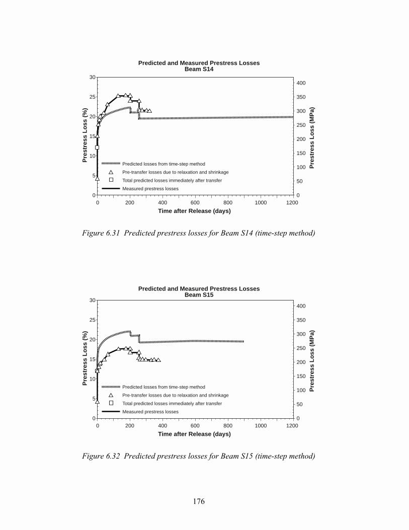
176
30
25
20
15
10
5
0
Pre
stre
ss L
oss
(%
)
0 200 400 600 800 1000 1200
Predicted losses from time-step method
Pre-transfer losses due to relaxation and shrinkage
Total predicted losses immediately after transfer
Measured prestress losses
Predicted and Measured Prestress LossesBeam S14
Time after Release (days)
400
350
300
250
200
150
100
50
0
Pre
stre
ss L
oss
(M
Pa)
Figure 6.31 Predicted prestress losses for Beam S14 (time-step method)
30
25
20
15
10
5
0
Pre
stre
ss L
oss
(%
)
0 200 400 600 800 1000 1200
Predicted losses from time-step method
Pre-transfer losses due to relaxation and shrinkage
Total predicted losses immediately after transfer
Measured prestress losses
Predicted and Measured Prestress LossesBeam S15
Time after Release (days)
400
350
300
250
200
150
100
50
0
Pre
stre
ss L
oss
(M
Pa)
Figure 6.32 Predicted prestress losses for Beam S15 (time-step method)

177
30
25
20
15
10
5
0
Pre
stre
ss L
oss
(%
)
0 200 400 600 800 1000 1200
Predicted losses from time-step method
Pre-transfer losses due to relaxation and shrinkage
Total predicted losses immediately after transfer
Measured prestress losses
Predicted and Measured Prestress LossesBeam S16
Time after Release (days)
400
350
300
250
200
150
100
50
0
Pre
stre
ss L
oss
(M
Pa)
Figure 6.33 Predicted prestress losses for Beam S16 (time-step method)
30
25
20
15
10
5
0
Pre
stre
ss L
oss
(%
)
0 200 400 600 800 1000 1200
Predicted losses from time-step method
Pre-transfer losses due to relaxation and shrinkage
Total predicted losses immediately after transfer
Measured prestress losses
Predicted and Measured Prestress LossesBeam S25
Time after Release (days)
400
350
300
250
200
150
100
50
0
Pre
stre
ss L
oss
(M
Pa)
Figure 6.34 Predicted prestress losses for Beam S25 (time-step method)
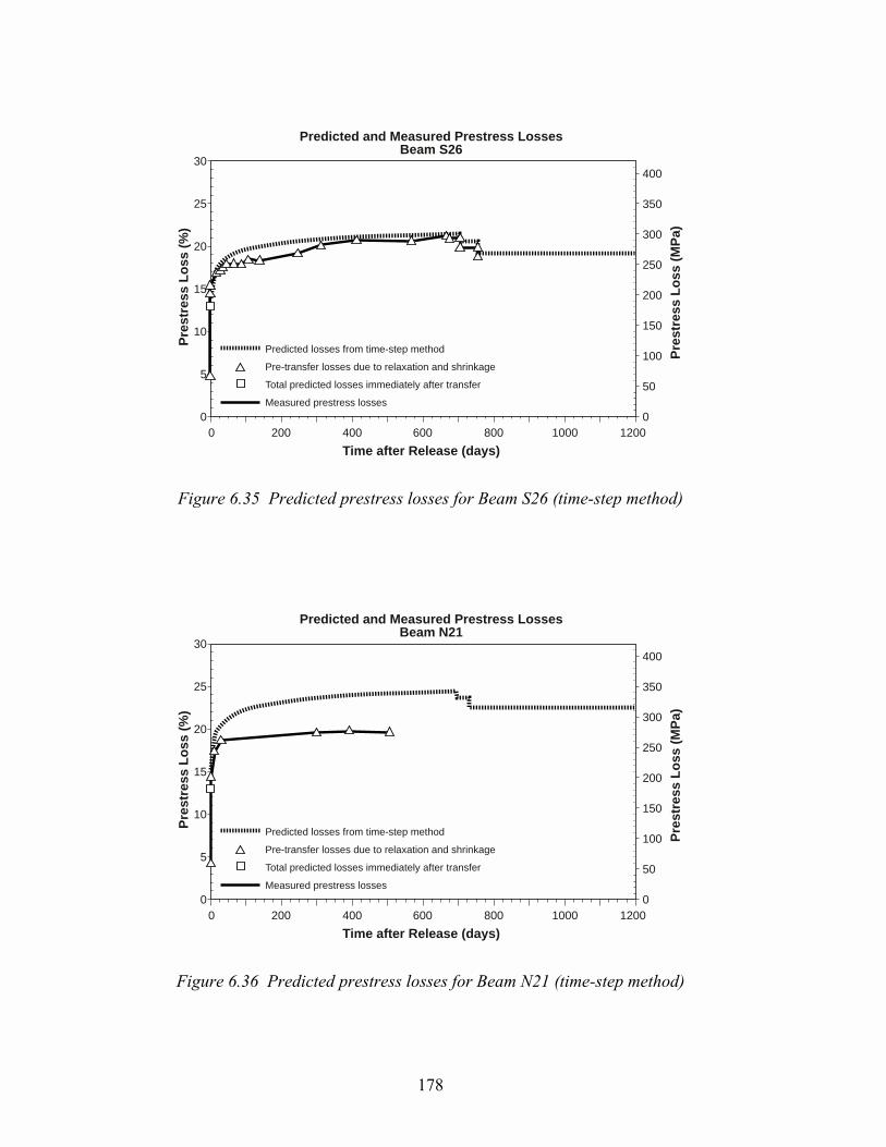
178
30
25
20
15
10
5
0
Pre
stre
ss L
oss
(%
)
0 200 400 600 800 1000 1200
Predicted losses from time-step method
Pre-transfer losses due to relaxation and shrinkage
Total predicted losses immediately after transfer
Measured prestress losses
Predicted and Measured Prestress LossesBeam S26
Time after Release (days)
400
350
300
250
200
150
100
50
0
Pre
stre
ss L
oss
(M
Pa)
Figure 6.35 Predicted prestress losses for Beam S26 (time-step method)
30
25
20
15
10
5
0
Pre
stre
ss L
oss
(%
)
0 200 400 600 800 1000 1200
Predicted losses from time-step method
Pre-transfer losses due to relaxation and shrinkage
Total predicted losses immediately after transfer
Measured prestress losses
Predicted and Measured Prestress LossesBeam N21
Time after Release (days)
400
350
300
250
200
150
100
50
0
Pre
stre
ss L
oss
(M
Pa)
Figure 6.36 Predicted prestress losses for Beam N21 (time-step method)

179
30
25
20
15
10
5
0
Pre
stre
ss L
oss
(%
)
0 200 400 600 800 1000 1200
Predicted losses from time-step method
Pre-transfer losses due to relaxation and shrinkage
Total predicted losses immediately after transfer
Measured prestress losses
Predicted and Measured Prestress LossesBeam N32
Time after Release (days)
400
350
300
250
200
150
100
50
0
Pre
stre
ss L
oss
(M
Pa)
Figure 6.37 Predicted prestress losses for Beam N32 (time-step method)
30
25
20
15
10
5
0
Pre
stre
ss L
oss
(%
)
0 200 400 600 800 1000 1200
Predicted losses from time-step method
Pre-transfer losses due to relaxation and shrinkage
Total predicted losses immediately after transfer
Measured prestress losses
Predicted and Measured Prestress LossesBeam N33
Time after Release (days)
400
350
300
250
200
150
100
50
0
Pre
stre
ss L
oss
(M
Pa)
Figure 6.38 Predicted prestress losses for Beam N33 (time-step method)
The initial losses before release that were calculated in the time-step method wereadded to all of the measured prestress losses. This was done because the baseline readingsfor the strain gages were taken just before release. As a result, any relaxation, shrinkage, or

180
temperature losses that occurred before release were not recorded by the gages. Themeasured losses did not include losses due to relaxation after release and no corrections weremade in Table 6.10 or in Figures 6.31 to 6.38 to account for this. The total additionalpredicted relaxation loss was approximately 0.5 percent.
The predicted elastic shortening losses varied between 6.80 percent (Beam N22) and8.83 percent (Beam N21). The measured elastic shortening losses varied between 6.28percent (Beam N22) and 12.10 percent (Beam S14). Generally, the largest measured elasticshortening losses were in Beams S26, N21, and N31, which had the largest prestressingforces. This was consistent with the predictions. Measured elastic shortening losses werehigher than the predicted losses for all of the beams except for Beams S15 and N22.
Total prestress losses after release, which are shown in Figures 6.31 to 6.38, weredetermined by adding the additional losses that were assumed to occur before release to theelastic shortening losses. These additional losses were approximately 4 percent for all of thebeams. Since the predicted losses before release were added to the measured values,comparisons between measured and predicted losses at any time were not affected.
The predicted prestress losses at erection varied between 20.83 percent (Beam S25)and 24.02 percent (Beam N21). As shown in Table 6.10, several of the instrumented beamsdid not have reliable long-term strain measurements. Therefore, predictions for those beamswere not included in the summary. The measured prestress losses at erection varied between17.77 percent (Beam S15) and 25.31 percent (Beam S14). With the exception of Beam S14,all of the measured prestress losses at erection were lower than the predicted losses.
Predicted increases in prestress losses from release to erection varied between 9.3percent (Beam S26) and 11.3 percent (Beam S16). The average predicted increase inprestress losses was 10.2 percent. Beam S26 exhibited low time-dependent prestress lossbecause the prestressing force was transferred at 7 days. Measured increases in prestresslosses varied between 6.7 percent (Beam S15) and 9.2 percent (Beam S14). The averagemeasured increase was only 7.1 percent. When the loss due to relaxation was added to themeasured values, the average difference was still nearly 2.5 percent.
For Beam S15, shown in Figure 6.32, the measured and predicted prestress losses atrelease were nearly the same but the predicted time-dependent increase in prestress loss wassignificantly larger than what was observed. Beams S16 and S25, shown in Figures 6.33 and6.34, respectively, had higher measured initial losses at release yet displayed smallerincreases in prestress losses up to erection. Similar trends were found in Beams S26 andN32, shown in Figures 6.35 and 6.37, respectively, although there was good agreementbetween measured and predicted losses at erection for these beams. Beam N21, shown inFigure 6.36, also exhibited higher measured losses at release followed by very little long-term growth. However, the measurements for this beam were probably unreliable after 100days.
The only beam to exhibit a measured time-dependent increase in prestress loss equalto the predicted increase was Beam S14. For this beam, the measured increase was 9.2percent while the predicted increase was 10.2 percent. After adding relaxation into themeasured loss, the predicted and measured growths agreed well. However, the measuredelastic shortening loss was much larger than the corresponding predicted loss.
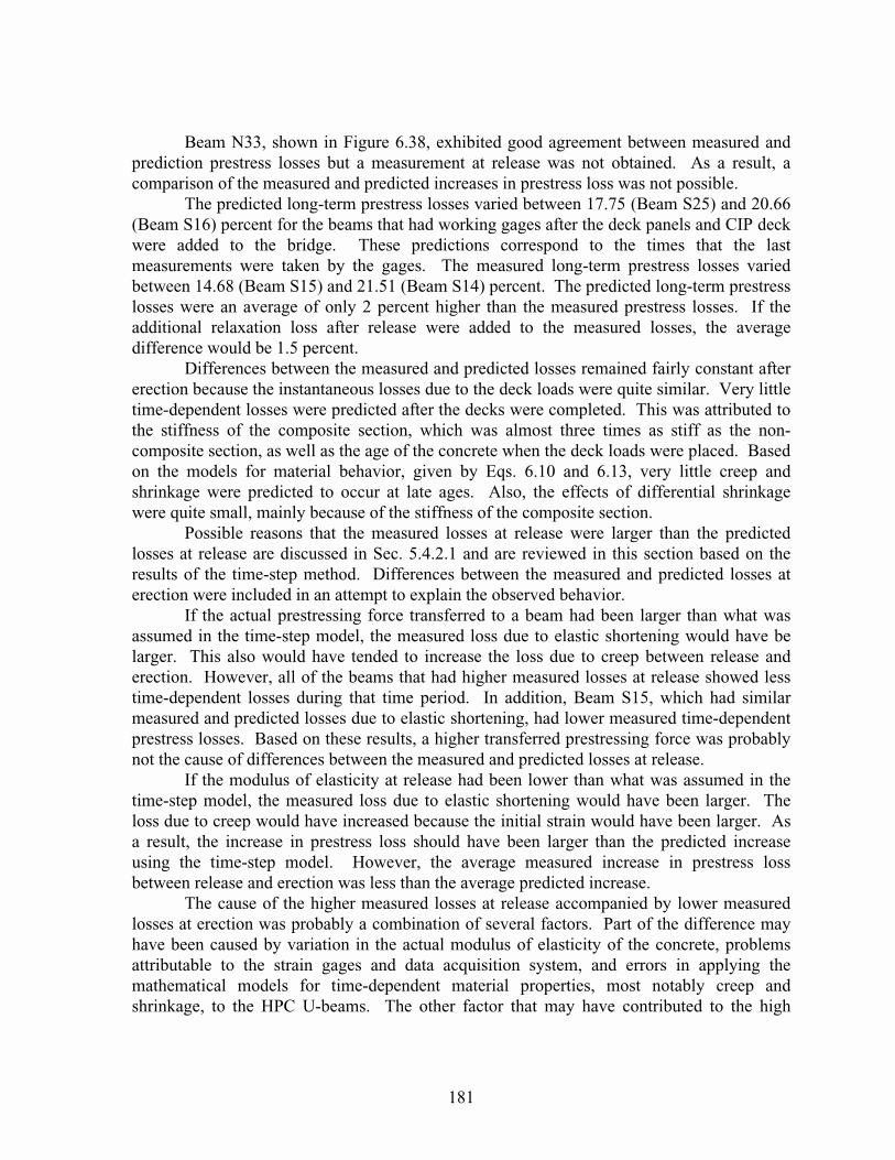
181
Beam N33, shown in Figure 6.38, exhibited good agreement between measured andprediction prestress losses but a measurement at release was not obtained. As a result, acomparison of the measured and predicted increases in prestress loss was not possible.
The predicted long-term prestress losses varied between 17.75 (Beam S25) and 20.66(Beam S16) percent for the beams that had working gages after the deck panels and CIP deckwere added to the bridge. These predictions correspond to the times that the lastmeasurements were taken by the gages. The measured long-term prestress losses variedbetween 14.68 (Beam S15) and 21.51 (Beam S14) percent. The predicted long-term prestresslosses were an average of only 2 percent higher than the measured prestress losses. If theadditional relaxation loss after release were added to the measured losses, the averagedifference would be 1.5 percent.
Differences between the measured and predicted losses remained fairly constant aftererection because the instantaneous losses due to the deck loads were quite similar. Very littletime-dependent losses were predicted after the decks were completed. This was attributed tothe stiffness of the composite section, which was almost three times as stiff as the non-composite section, as well as the age of the concrete when the deck loads were placed. Basedon the models for material behavior, given by Eqs. 6.10 and 6.13, very little creep andshrinkage were predicted to occur at late ages. Also, the effects of differential shrinkagewere quite small, mainly because of the stiffness of the composite section.
Possible reasons that the measured losses at release were larger than the predictedlosses at release are discussed in Sec. 5.4.2.1 and are reviewed in this section based on theresults of the time-step method. Differences between the measured and predicted losses aterection were included in an attempt to explain the observed behavior.
If the actual prestressing force transferred to a beam had been larger than what wasassumed in the time-step model, the measured loss due to elastic shortening would have belarger. This also would have tended to increase the loss due to creep between release anderection. However, all of the beams that had higher measured losses at release showed lesstime-dependent losses during that time period. In addition, Beam S15, which had similarmeasured and predicted losses due to elastic shortening, had lower measured time-dependentprestress losses. Based on these results, a higher transferred prestressing force was probablynot the cause of differences between the measured and predicted losses at release.
If the modulus of elasticity at release had been lower than what was assumed in thetime-step model, the measured loss due to elastic shortening would have been larger. Theloss due to creep would have increased because the initial strain would have been larger. Asa result, the increase in prestress loss should have been larger than the predicted increaseusing the time-step model. However, the average measured increase in prestress lossbetween release and erection was less than the average predicted increase.
The cause of the higher measured losses at release accompanied by lower measuredlosses at erection was probably a combination of several factors. Part of the difference mayhave been caused by variation in the actual modulus of elasticity of the concrete, problemsattributable to the strain gages and data acquisition system, and errors in applying themathematical models for time-dependent material properties, most notably creep andshrinkage, to the HPC U-beams. The other factor that may have contributed to the high

182
measured release losses was restraint offered by the prestressing bed during extreme thermalcooling that occurred in the beams after hydration. This concept is discussed extensively inSec. 5.4.2.1. This effect may have made the measured strains at release artificially high dueto the measurement of additional strain in the beams caused by restraint of the bed duringuneven cooling of the section. This effect would not have changed the amount of time-dependent prestress losses observed in the HPC U-beams. In addition, the creep andshrinkage losses in the time-step model probably slightly overestimated the actual behavior.
6.4.3 Camber and Deflection
6.4.3.1 Analytical Procedure
The analytical procedure for predicting the time-dependent camber and deflectionresponse for the instrumented beams involved determining elastic camber or deflection due toapplied loads and then calculating time-dependent increases in the elastic responses for afinite number of time intervals. The time-dependent portion of the response was determinedby applying differential creep coefficients to the elastic responses over each discrete timeinterval. Additional consideration was given to the loss of prestress over time and to theeffect of differential shrinkage, which are outlined in Sec. 6.4.2.1.
The calculation of elastic camber due to the prestressing force included the effect ofstrand debonding. Since the debonding patterns, which are found in Appendix A, were quitecomplicated, a formula for the camber due to prestress is not shown. The values for modulusof elasticity and transformed section properties were identical to those used for calculatingelastic shortening. In addition, the stress in the strands was identical to the predicted stressjust after release, which included the losses that occurred before release. This was discussedin Sec. 6.4.2.1.
The elastic deflection due to the beam weight was calculated using Eqs. 6.4 and 6.5,which are given in Sec. 6.3.2.1. The material and section properties used for this calculationwere the same as those used in the calculation of elastic camber due to the prestressing force.
The elastic deflections due to the deck panels and the cast-in-place (CIP) deck werecalculated using Eq. 6.8, which is given in Sec. 6.3.2.1. The actual times of the events,which are given in Sec. 4.3.1, and Eqs. 6.11 and 6.12, shown in Sec. 6.4.2.1, were used tocalculate the material properties. Transformed section properties were calculated based onthe modular ratio of prestressing steel to concrete at the time of loading. The loads werebased on the measured deck thicknesses. These loads are summarized in Table 6.5.
Time-dependent components of camber and deflection were calculated using Eqs.6.18 and 6.19, respectively. These expressions represent changes in camber and deflectionover a discrete time interval based on the incremental creep coefficient, the average loss ofprestress force at that time, and the elastic components of camber and deflection. Equation6.18 also includes the incremental reduction in the elastic prestress component due to theincremental reduction in the prestressing force over each time interval.

183
� � � � � �� � � �
�� �
� �
)
� �
)
� � � � ��
0 0
0
0 0
0. .� �
��
��
�
� � �
��
��
�
� �
�
�
�
��� �
�� �
��
�������������
� � � � � � � �� � �& � ��! ��/�& .�� � � � �. . ���������������������������������������������� � � �
��
wheret = end of time interval i (time after release)� = differential length of time for interval iFt = loss of prestressing force after release at time tFt-� = loss of prestressing force after release at time (t-�)Fo = prestressing force immediately after releaseCc = creep coefficient at times t and (t-�) calculated using Eq. 6.13ps = initial camber due to prestressing force, Fo
beam = initial deflection due to beam weightpanel = initial deflection due to deck panelsCIP = initial deflection due to cast-in-place deck
In Eq. 6.19, panel and CIP will be zero for all time intervals that occur before the timeof placement of these loads on the beams. Once the beam section becomes composite, theincremental components of camber and deflection shown in Eqs. 6.19 and 6.20 are multipliedby the ratio of non-composite to composite moments of inertia. The assumptions made inSec. 6.4.2.1 concerning calculation of transformed section properties for the compositesection apply to the calculations presented in this section. The total camber or deflection atany time is given by Eq. 6.20.
� � � � � �� � � �� ��! ��/�& .�� �� � �& � �����"# ��
/
��������������������� � � � � � ���
�
wheret = time after release in days (corresponds to the end of time interval n)n = number of time intervals used to reach time tdiffshr = deflection due to differential shrinkage between the deck and the
beam during the time interval I
In Eq. 6.20, panel and CIP may equal zero if time t is before placement of these loadson the beam. Also, the deflection due to differential shrinkage, diffshr, will be zero at any timebefore placement of the CIP deck. The equation for differential shrinkage was not includedin this section but its effect was shown in Eq. 6.20. Branson and Kripanarayanan (43)provided an equation that was used in conjunction with the assumed ultimate deck shrinkages
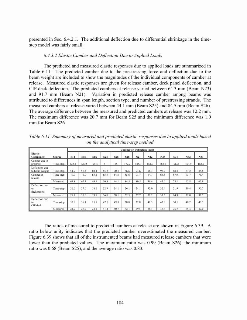
184
presented in Sec. 6.4.2.1. The additional deflection due to differential shrinkage in the time-step model was fairly small.
6.4.3.2 Elastic Camber and Deflection Due to Applied Loads
The predicted and measured elastic responses due to applied loads are summarized inTable 6.11. The predicted camber due to the prestressing force and deflection due to thebeam weight are included to show the magnitudes of the individual components of camber atrelease. Measured elastic responses are given for release camber, deck panel deflection, andCIP deck deflection. The predicted cambers at release varied between 64.3 mm (Beam N23)and 91.7 mm (Beam N21). Variation in predicted release camber among beams wasattributed to differences in span length, section type, and number of prestressing strands. Themeasured cambers at release varied between 44.1 mm (Beam S25) and 84.5 mm (Beam S26).The average difference between the measured and predicted cambers at release was 12.2 mm.The maximum difference was 20.7 mm for Beam S25 and the minimum difference was 1.0mm for Beam S26.
Table 6.11 Summary of measured and predicted elastic responses due to applied loads basedon the analytical time-step method
Camber or Deflection (mm)ElasticComponent Source S14 S15 S16 S24 S25 S26 N21 N22 N23 N31 N32 N33Camber due toprestress Time-step 122.8 126.2 125.5 151.1 155.1 172.2 185.3 161.0 162.5 176.2 160.9 162.2Deflection dueto beam weight Time-step 51.9 55.3 60.4 85.2 90.3 86.6 93.6 96.3 98.2 88.3 87.2 88.8Camber atrelease
Time-step 70.9 70.9 65.1 65.9 64.8 85.6 91.7 64.7 64.3 87.9 73.7 73.4
Measured 61.8 62.4 49.1 50.8 44.1 84.5 80.5 46.4 45.0 78.1 63.8 65.9Deflection duetodeck panels
Time-step 26.0 27.0 18.6 32.9 34.1 26.1 24.1 32.0 32.4 21.9 30.4 30.7
Measured 29.7 30.0 19.8 36.0 38.1 32.5 27.7 32.2 33.3 24.9 32.0 32.7Deflection duetoCIP deck
Time-step 32.9 36.1 25.9 47.5 49.3 38.8 32.8 42.3 42.9 30.1 40.2 40.7
Measured 24.9 28.7 24.1 41.4 40.7 32.1 29.5 38.1 35.3 26.7 35.3 32.0
The ratios of measured to predicted cambers at release are shown in Figure 6.39. Aratio below unity indicates that the predicted camber overestimated the measured camber.Figure 6.39 shows that all of the instrumented beams had measured release cambers that werelower than the predicted values. The maximum ratio was 0.99 (Beam S26), the minimumratio was 0.68 (Beam S25), and the average ratio was 0.83.

185
1.4
1.2
1.0
0.8
0.6
0.4
0.2
0.0
Mea
sure
d/P
red
icte
d
S14 S15 S16 S24 S25 S26 N21 N22 N23 N31 N32 N33
Deck panel deflection
CIP deck deflection
Release camber
Predicted Elastic Responses Using Time-Step Method
Figure 6.39 Summary of the ratios of measured to predicted elastic responses using thetime-step method
Consistently low camber at release did not agree with the consistently high measuredelastic shortening losses shown in Sec. 6.4.2.2. Low measured camber implied the followingdifferences, alone or in combination, between actual conditions during the measurements andthe assumptions used in the time-step method:
1.� Higher modulus of elasticity2.� Lower prestressing force transferred to the beam3.� Increased beam self-weight
These differences would have caused the measured elastic shortening loss to becomesmaller rather than larger. This observation supports the idea that additional strain due torestraint offered by the bed during cooling of the beam was being measured at release. Sincethe measured elastic shortening losses appeared to be distorted in this way, it was difficult toverify the cause of low measured cambers at release.
The predicted deflections due to the deck panels varied between 18.6 mm (Beam S16)and 34.1 mm (Beam S25). The predicted deflections were the largest for beams with thelargest spacing and span length. The predicted deflections were the smallest for the exteriorbeams. The measured deflections due to deck panels varied from 19.8 mm (Beam S16) to38.1 mm (Beam S25). The average difference between measured and predicted deflectionswas only 2.7 mm. The maximum difference was 6.4 mm (Beam S26) and the minimumdifference was 0.2 mm (Beam N22).
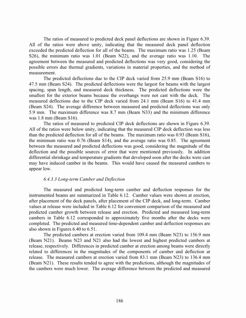
186
The ratios of measured to predicted deck panel deflections are shown in Figure 6.39.All of the ratios were above unity, indicating that the measured deck panel deflectionexceeded the predicted deflection for all of the beams. The maximum ratio was 1.25 (BeamS26), the minimum ratio was 1.01 (Beam N22), and the average ratio was 1.10. Theagreement between the measured and predicted deflections was very good, considering thepossible errors due thermal gradients, variations in material properties, and the method ofmeasurement.
The predicted deflections due to the CIP deck varied from 25.9 mm (Beam S16) to47.5 mm (Beam S24). The predicted deflections were the largest for beams with the largestspacing, span length, and measured deck thickness. The predicted deflections were thesmallest for the exterior beams because the overhangs were not cast with the deck. Themeasured deflections due to the CIP deck varied from 24.1 mm (Beam S16) to 41.4 mm(Beam S24). The average difference between measured and predicted deflections was only5.9 mm. The maximum difference was 8.7 mm (Beam N33) and the minimum differencewas 1.8 mm (Beam S16).
The ratios of measured to predicted CIP deck deflections are shown in Figure 6.39.All of the ratios were below unity, indicating that the measured CIP deck deflection was lessthan the predicted deflection for all of the beams. The maximum ratio was 0.93 (Beam S16),the minimum ratio was 0.76 (Beam S14), and the average ratio was 0.85. The agreementbetween the measured and predicted deflections was good, considering the magnitude of thedeflection and the possible sources of error that were mentioned previously. In additiondifferential shrinkage and temperature gradients that developed soon after the decks were castmay have induced camber in the beams. This would have caused the measured cambers toappear low.
6.4.3.3 Long-term Camber and Deflection
The measured and predicted long-term camber and deflection responses for theinstrumented beams are summarized in Table 6.12. Camber values were shown at erection,after placement of the deck panels, after placement of the CIP deck, and long-term. Cambervalues at release were included in Table 6.12 for convenient comparison of the measured andpredicted camber growth between release and erection. Predicted and measured long-termcambers in Table 6.12 corresponded to approximately five months after the decks werecompleted. The predicted and measured time-dependent camber and deflection responses arealso shown in Figures 6.40 to 6.51.
The predicted cambers at erection varied from 109.4 mm (Beam N23) to 156.9 mm(Beam N21). Beams N23 and N21 also had the lowest and highest predicted cambers atrelease, respectively. Differences in predicted camber at erection among beams were directlyrelated to differences in the magnitudes of the components of camber and deflection atrelease. The measured cambers at erection varied from 83.1 mm (Beam N23) to 136.4 mm(Beam N21). These results tended to agree with the predictions, although the magnitudes ofthe cambers were much lower. The average difference between the predicted and measured
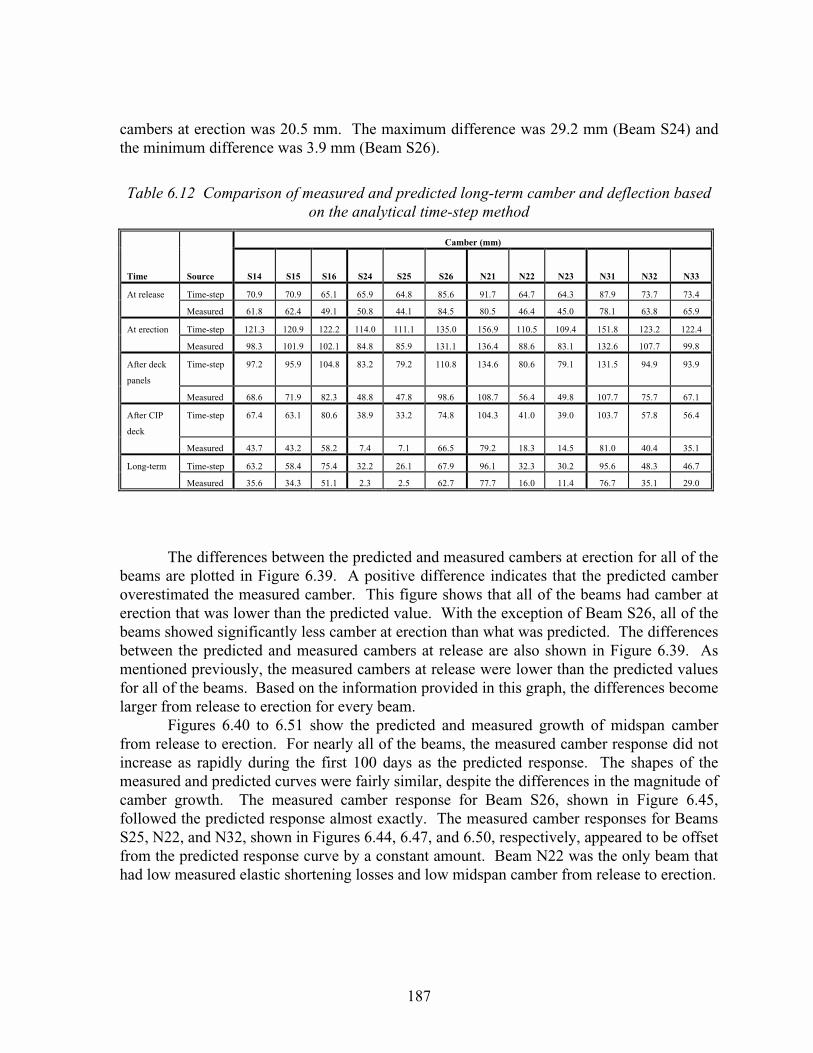
187
cambers at erection was 20.5 mm. The maximum difference was 29.2 mm (Beam S24) andthe minimum difference was 3.9 mm (Beam S26).
Table 6.12 Comparison of measured and predicted long-term camber and deflection basedon the analytical time-step method
Camber (mm)
Time Source S14 S15 S16 S24 S25 S26 N21 N22 N23 N31 N32 N33
At release Time-step 70.9 70.9 65.1 65.9 64.8 85.6 91.7 64.7 64.3 87.9 73.7 73.4
Measured 61.8 62.4 49.1 50.8 44.1 84.5 80.5 46.4 45.0 78.1 63.8 65.9
At erection Time-step 121.3 120.9 122.2 114.0 111.1 135.0 156.9 110.5 109.4 151.8 123.2 122.4
Measured 98.3 101.9 102.1 84.8 85.9 131.1 136.4 88.6 83.1 132.6 107.7 99.8
After deck
panels
Time-step 97.2 95.9 104.8 83.2 79.2 110.8 134.6 80.6 79.1 131.5 94.9 93.9
Measured 68.6 71.9 82.3 48.8 47.8 98.6 108.7 56.4 49.8 107.7 75.7 67.1
After CIP
deck
Time-step 67.4 63.1 80.6 38.9 33.2 74.8 104.3 41.0 39.0 103.7 57.8 56.4
Measured 43.7 43.2 58.2 7.4 7.1 66.5 79.2 18.3 14.5 81.0 40.4 35.1
Long-term Time-step 63.2 58.4 75.4 32.2 26.1 67.9 96.1 32.3 30.2 95.6 48.3 46.7
Measured 35.6 34.3 51.1 2.3 2.5 62.7 77.7 16.0 11.4 76.7 35.1 29.0
The differences between the predicted and measured cambers at erection for all of thebeams are plotted in Figure 6.39. A positive difference indicates that the predicted camberoverestimated the measured camber. This figure shows that all of the beams had camber aterection that was lower than the predicted value. With the exception of Beam S26, all of thebeams showed significantly less camber at erection than what was predicted. The differencesbetween the predicted and measured cambers at release are also shown in Figure 6.39. Asmentioned previously, the measured cambers at release were lower than the predicted valuesfor all of the beams. Based on the information provided in this graph, the differences becomelarger from release to erection for every beam.
Figures 6.40 to 6.51 show the predicted and measured growth of midspan camberfrom release to erection. For nearly all of the beams, the measured camber response did notincrease as rapidly during the first 100 days as the predicted response. The shapes of themeasured and predicted curves were fairly similar, despite the differences in the magnitude ofcamber growth. The measured camber response for Beam S26, shown in Figure 6.45,followed the predicted response almost exactly. The measured camber responses for BeamsS25, N22, and N32, shown in Figures 6.44, 6.47, and 6.50, respectively, appeared to be offsetfrom the predicted response curve by a constant amount. Beam N22 was the only beam thathad low measured elastic shortening losses and low midspan camber from release to erection.

188
140
120
100
80
60
40
20
0
Mid
span
Cam
ber
(m
m)
0 100 200 300 400 500 600 700 800
Predicted and Measured Camber ResponseBeam S14
Time after Release (days)
Predicted response using time-step method
Measured response
1. Immediately after release
2. Precast deck panel erection
3. Casting of CIP deck
1
2
3
Figure 6.40 Predicted camber for Beam S14 using the time-step method
140
120
100
80
60
40
20
0
Mid
span
Cam
ber
(m
m)
0 100 200 300 400 500 600 700 800
Predicted and Measured Camber ResponseBeam S15
Time after Release (days)
Predicted response using time-step method
Measured response
1. Immediately after release
2. Precast deck panel erection
3. Casting of CIP deck
1
2
3
Figure 6.41 Predicted camber for Beam S15 using the time-step method
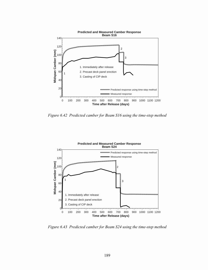
189
140
120
100
80
60
40
20
0
Mid
span
Cam
ber
(m
m)
0 100 200 300 400 500 600 700 800 900 1000 1100 1200
Predicted and Measured Camber ResponseBeam S16
Time after Release (days)
Predicted response using time-step method
Measured response
1. Immediately after release
2. Precast deck panel erection
3. Casting of CIP deck1
2
3
Figure 6.42 Predicted camber for Beam S16 using the time-step method
140
120
100
80
60
40
20
0
Mid
span
Cam
ber
(m
m)
0 100 200 300 400 500 600 700 800 900 1000 1100 1200
Predicted and Measured Camber ResponseBeam S24
Time after Release (days)
Predicted response using time-step method
Measured response
1. Immediately after release
2. Precast deck panel erection
3. Casting of CIP deck
1
2
3
Figure 6.43 Predicted camber for Beam S24 using the time-step method
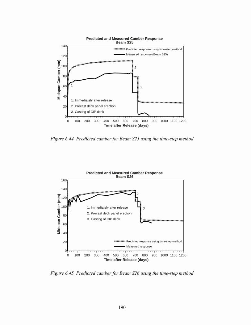
190
140
120
100
80
60
40
20
0
Mid
span
Cam
ber
(m
m)
0 100 200 300 400 500 600 700 800 900 1000 1100 1200
Predicted and Measured Camber ResponseBeam S25
Time after Release (days)
Predicted response using time-step method
Measured response (Beam S25)
1. Immediately after release
2. Precast deck panel erection
3. Casting of CIP deck
1
2
3
Figure 6.44 Predicted camber for Beam S25 using the time-step method
160
140
120
100
80
60
40
20
0
Mid
span
Cam
ber
(m
m)
0 100 200 300 400 500 600 700 800 900 1000 1100 1200
Predicted and Measured Camber ResponseBeam S26
Time after Release (days)
Predicted response using time-step method
Measured response
1. Immediately after release
2. Precast deck panel erection
3. Casting of CIP deck
1
2
3
Figure 6.45 Predicted camber for Beam S26 using the time-step method

191
180
160
140
120
100
80
60
40
20
0
Mid
span
Cam
ber
(m
m)
0 100 200 300 400 500 600 700 800 900 1000 1100 1200
Predicted and Measured Camber ResponseBeam N21
Time after Release (days)
Predicted response using time-step method
Measured response
1. Immediately after release
2. Precast deck panel erection
3. Casting of CIP deck
1
2
3
Figure 6.46 Predicted camber for Beam N21 using the time-step method
140
120
100
80
60
40
20
0
Mid
span
Cam
ber
(m
m)
0 100 200 300 400 500 600 700 800 900 1000 1100 1200
Predicted and Measured Camber ResponseBeam N22
Time after Release (days)
Predicted response using time-step method
Measured response
1. Immediately after release
2. Precast deck panel erection
3. Casting of CIP deck
1
2
3
Figure 6.47 Predicted camber for Beam N22 using the time-step method

192
140
120
100
80
60
40
20
0
Mid
span
Cam
ber
(m
m)
0 100 200 300 400 500 600 700 800 900 1000 1100 1200
Predicted and Measured Camber ResponseBeam N23
Time after Release (days)
Predicted response using time-step method
Measured response
1. Immediately after release
2. Precast deck panel erection
3. Casting of CIP deck
1
2
3
Figure 6.48 Predicted camber for Beam N23 using the time-step method
180
160
140
120
100
80
60
40
20
0
Mid
span
Cam
ber
(m
m)
0 100 200 300 400 500 600 700 800 900 1000 1100 1200
Predicted and Measured Camber ResponseBeam N31
Time after Release (days)
Predicted response using time-step method
Measured response
1. Immediately after release
2. Precast deck panel erection
3. Casting of CIP deck
1
2
3
Figure 6.49 Predicted camber for Beam N31 using the time-step method
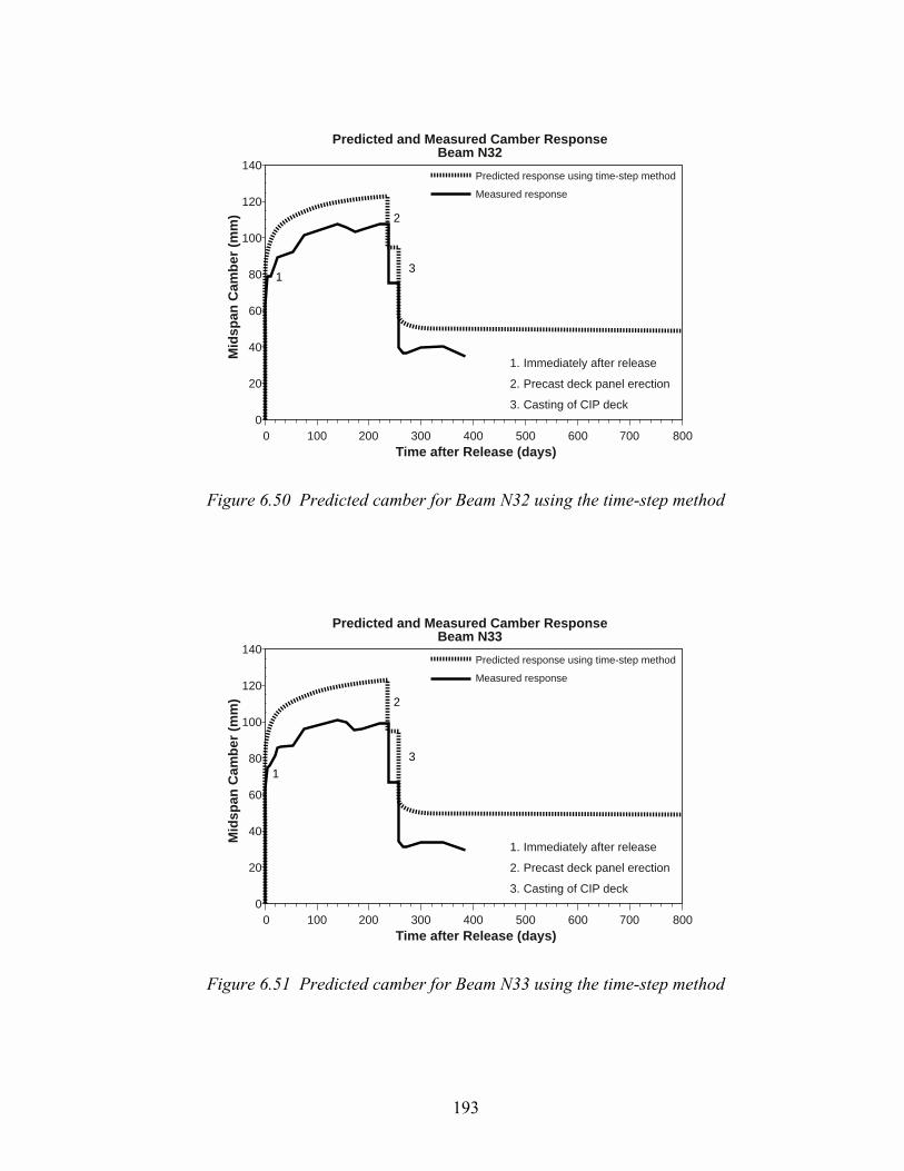
193
140
120
100
80
60
40
20
0
Mid
span
Cam
ber
(m
m)
0 100 200 300 400 500 600 700 800
Predicted and Measured Camber ResponseBeam N32
Time after Release (days)
Predicted response using time-step method
Measured response
1. Immediately after release
2. Precast deck panel erection
3. Casting of CIP deck
1
2
3
Figure 6.50 Predicted camber for Beam N32 using the time-step method
140
120
100
80
60
40
20
0
Mid
span
Cam
ber
(m
m)
0 100 200 300 400 500 600 700 800
Predicted and Measured Camber ResponseBeam N33
Time after Release (days)
Predicted response using time-step method
Measured response
1. Immediately after release
2. Precast deck panel erection
3. Casting of CIP deck
1
2
3
Figure 6.51 Predicted camber for Beam N33 using the time-step method
194
The average predicted and measured growths of midspan camber from release toerection were 51.7 mm and 43.3 mm, respectively. Low measured camber growth was due toa combination of several possible differences between actual conditions and the analyticalmodel. Some of these possible differences include a higher modulus of elasticity at release, alower ultimate creep coefficient than what used in the analytical model, and a lowerprestressing force transferred to the beams.
Another possible cause for low measured camber from release to erection may havebeen the effect of early age thermal gradients that developed during hydration. Temperaturemeasurements for Beams S16 and N32 during casting showed the formation of temperaturegradient as large as 9 °C between the top and bottom of the beam. After the side forms areremoved, the beams will eventually cool to a uniform temperature, causing the top to shortenmore than the bottom. The result of this uneven cooling, where the top cools more than thebottom, would be a negative curvature. This would cause a component of deflection. Thiscomponent of deflection would be present in every camber measurement from releasethrough long-term because the measurements were only corrected for thermal gradientsreferenced to a uniform gradient, as discussed in Sec. 5.3.1. The proper adjustment may beto use the temperature gradient at some time before the forms are stripped as the referencegradient.
Unfortunately, very few beams were monitored during casting, so corrections basedan early-age temperature gradient were not attempted. The magnitude of this correctionbased on the gradients observed in Beams S16 and N32 could have been as large as 12 mm,depending on the length of the beam. Offsets of this magnitude were present between nearlyall of the predicted and measured camber responses shown in Figures 6.40 to 6.51.
The predicted cambers after placement of the CIP deck varied from 33.2 mm (BeamS25) to 104.3 mm (Beam N21). The interior beams, which had the longest spans, had thelowest cambers at this point. The exterior beams had the highest cambers because theoverhangs were not cast with the deck. The measured cambers after placement of the CIPdeck varied from 7.1 mm (Beam S25) to 81.0 mm (Beam N31). The average differencebetween the measured and predicted cambers at this point was 22.1 mm. This was very closeto the average difference before erection because the measured and predicted elasticdeflections were so close, as shown in Sec. 6.4.3.2.
The predicted long-term cambers varied from 26.1 mm (Beam S25) to 96.1 mm(Beam N21). These values corresponded to the time of the last measured camber for eachbeam. The predicted long-term camber, shown in Figures 6.40 to 6.51, did not changesignificantly after the beam section became composite. This was because of the increasedstiffness of the section and the small amount of creep occurring at those late ages. Theobserved decrease in camber was mainly due to differential shrinkage between the CIP deckand the beam. The measured long-term cambers varied from 2.3 mm (Beam S24) to 77.7mm (Beam N21). The average difference between the measured and predicted long-termcamber was 19.8 mm. The maximum difference was 29.9 mm (Beam S24) and the minimumdifference was 5.2 mm (Beam S26).
The differences between the predicted and measured long-term cambers for all of thebeams are plotted in Figure 6.52. A positive difference indicates that the predicted camber

195
overestimated the measured camber. This figure shows that all of the beams had long-termcamber that was lower than the predicted value. The long-term camber differences were verysimilar to the differences observed at erection. Based on all of the plots shown in Figure6.52, measured camber was consistently low from release through long-term for all of thebeams. Furthermore, the differences remained fairly close for some of the beams fromrelease to erection and then they remained very close for all of the beams through long-termmeasurements.
40
35
30
25
20
15
10
5
0
Pre
dic
ted
- M
easu
red
(m
m)
S14 S15 S16 S24 S25 S26 N21 N22 N23 N31 N32 N33
Camber at release
At erection
Long-term
Predicted Long-Term Responses Using Time-Step Method
Figure 6.52 Summary of differences between measured and predicted long-term camber anddeflection based on the time-step method
6.5 PROPOSED MULTIPLIERS FOR ESTIMATING TIME-DEPENDENTCAMBER AND DEFLECTION
6.5.1 Development of Proposed Multipliers
In this section, a set of camber and deflection multipliers are developed for predictingthe time-dependent behavior of prestressed high performance concrete U-beams. The ideasused to develop these multipliers are comparable to those used by Martin (28). Theanalytical approach is based on the time-step method presented in Sec. 6.4, which was similarto the analytical technique presented by Branson and Kripanarayanana (43).
Time-dependent growth of camber is basically a function of creep and loss ofprestress. Since creep is a function of several parameters, including volume-to-surface ratioand relative humidity, accurate prediction of long-term camber and deflection is extremelydifficult. The material models for creep, shrinkage, compressive strength, and modulus of
196
elasticity that were used in the time-step method predicted the time-dependent behavior ofthe U-beams with acceptable accuracy. The general shape of the predicted camber responsescoincided with the measured camber responses, although the measured responses for most ofthe beams were consistently low from release to several months after completion of thecomposite decks.
At release, a prestressed concrete beam experiences an upward deflection, or camber,due to the prestressing force, and a downward deflection due to the beam weight. Theaddition of these two deflections represents the initial camber at release. This relationship isshown in Eq. 6.21.
� � � � � �� � ��! �������������������������������������������������� �
The initial components of upward and downward deflection at release are elasticresponses that happen over a short period of time. As time progresses, these components ofdeflection increase in magnitude due to creep of the concrete. The camber of a beam at anytime after release, without the addition of superimposed loads, is shown in Eq. 6.22.
� � � � � �� �� � � ��! ����������������������������������������������� �� �
The coefficients �pt and �bt are multipliers of the elastic components of deflection.Their values are greater than unity to account for both the elastic and time-dependent parts ofthe deflection. As shown in Eq. 6.23, the magnitude of each multiplier is dependent uponseveral factors (�j). The factors account for the influences that time-dependent properties andchanges in geometric properties have on the increase of deflection components.
� �1 1, � % ����������������������������������������������������������� �
The factor that represents the time function used to model the increase in concretecreep and prestress loss is given by Eq. 6.24. The factor that accounts for the increasedmoment of inertia when the beam section becomes composite is given by Eq. 6.25. For theU-beams in this study, �I was taken as 0.35.
�2
��
��
�
� ���������������������������������������������������������
�
�
��
�
�
� �/�
�
�
���������������������������������������������������������������� ��
The time-dependent deflection due to the weight of the beam is only a function ofcreep. The value for the ultimate creep coefficient, �cu, was taken as 1.40 for all of the U-
197
beams except Beam S26. For that beam, �cu was taken as 1.05 because transfer occurred 7days after casting. The deflection due to the weight of the beam at any time after release isshown in Eq. 6.26. The multiplier for the beam weight deflection, �bt, is shown in Eq. 6.27.If the beam section were to remain non-composite through the end of its service life, �bt
would be equal to one plus the ultimate creep coefficient.
� � � � � � ��! � ��! � 2 �+ ������������������������������� ���� � �
� � � � 2 �+, % �������������������������������������������������������
Once the beam section becomes composite, the moment of inertia increases. Thefactor to account for the increase in moment of inertia is shown in Eq. 6.25. The time-dependent increase in the beam weight deflection that occurs after the beam becomescomposite will be reduced by this increase in stiffness. To determine the beam weightmultiplier after the beam section becomes composite, the fraction of creep that has occurredup to that point needs to be calculated. The multiplier for beam weight deflection before thebeam becomes composite is given in Eq. 6.28.
� �� � � /� 2 /� �+, % ������������������������������������������������
The multiplier for beam weight deflection at any time after the beam section becomescomposite is shown in Eq. 6.29. The time-dependent fraction of creep that has occurredbefore the section becomes composite is represented by �bnc. The time-dependent creep thatoccurs after the composite section is represented by the second term in Eq. 6.29.
� �� �� � � � � � �� /� 2 2 /� � �+, % ���������������������������������������
The time-dependent increase in camber due to the prestressing force is a function ofcreep and prestress losses after release. Since creep is a large contributor to prestress lossesafter release, the time factor shown in Eq. 6.24 was used to represent the time-dependent lossof prestress. The value for the total loss of prestress after release, �pl, was taken as 12 percent(expressed as a decimal) for all of the U-beams.
The camber due to prestressing any time after release is shown in Eq. 6.30. Themultiplier for the camber due to prestress, �pt, is shown in Eq. 6.31. �pt will always be lessthan �bt because the initial component of camber, (ps)i, is reduced by the total loss ofprestress (1-�pl). (Ps)i is also directly reduced by the loss of prestress over time, which isrepresented by the term (�T�pl�E). �E, given in Eq. 6.32, is a factor that accounts for theincrease in modulus of elasticity with time. The value of �E was taken as 0.90 for the HPCU-beams.
198
� � � � � �� � �� � �� � 2 �+ 2 �& 2 �& �% ���������������������������� � ���� �� � � � � � ���
� �� � � � � � � ��� 2 �+ 2 �& 2 �& �, % ��� � � �������������������������������������������������
� �� �
��
� ��
�
�����������������������������������������������������������
The influence of the composite moment of inertia on the time-dependent camber dueto the prestressing force is similar to that shown for the deflection due to the beam weight.The factor to account for the increase in moment of inertia (�I) is shown in Eq. 6.25. Thetime-dependent increase in the camber due to the prestressing force that occurs after the beambecomes composite will be reduced by the increase in stiffness. To determine the multiplierafter the beam section becomes composite, the fraction of creep that has occurred up to thatpoint needs to be calculated. The multiplier for prestress camber before the beam becomescomposite is shown in Eq. 6.33.
� � � �� �� �� � � � � � ��/� 2 /� �+ 2 /� �& �& �, % ��� � � � ���������������������������������������
The multiplier for camber due to the prestressing force at any time after the beamsection becomes composite is shown in Eq. 6.34. The fraction of creep that has occurredbefore the section becomes composite is represented by �pnc. The time-dependent creep thatoccurs after the composite section is represented by the second term in Eq. 6.34.
� �� � � �� �� � � � � � � � � ���� �/� 2 2 /� � �+ 2 �& �& �, % ��� � � ������������������������������
Multipliers for the time-dependent deflections due to superimposed deck panels andcast-in-place deck loads are developed similarly to the beam weight multiplier. Deflectionsdue to superimposed loads are only a function of creep. The amount of additional time-dependent deflection due to creep will be determined by the age of loading. The deflectiondue to a superimposed dead load at any time after its placement on the beam is given by Eq.6.35. This equation was developed using the time factor (�T) given in Eq. 6.24, the momentof inertia factor (�I) given in Eq. 6.25, and the ultimate creep coefficient (�cu). The fraction ofcreep that occurs before the beam section becomes composite is represented by (�T)nc. Thisequation assumes that no time occurs between placement of the deck panels and casting ofthe deck slab. The dead load multiplier at any time after placement is given by Eq. 6.36.
� � � � � �� �� � �& � �& � 2 2 /� �+ � ������������������������������� �� � ���� � � � �
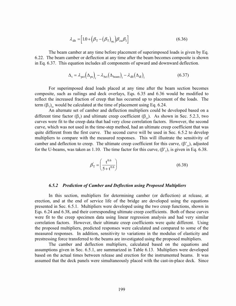
199
� �� �� �� � � � ��&� 2 2 /� �+ � ������������������������������������������������ � ����
The beam camber at any time before placement of superimposed loads is given by Eq.6.22. The beam camber or deflection at any time after the beam becomes composite is shownin Eq. 6.37. This equation includes all components of upward and downward deflection.
� � � � � � � ��� �� � �� ��! � �&� �& ����������������������������������� � �� � �
For superimposed dead loads placed at any time after the beam section becomescomposite, such as railings and deck overlays, Eqs. 6.35 and 6.36 would be modified toreflect the increased fraction of creep that has occurred up to placement of the loads. Theterm (�T)nc would be calculated at the time of placement using Eq. 6.24.
An alternate set of camber and deflection multipliers could be developed based on adifferent time factor (�T) and ultimate creep coefficient (�cu). As shown in Sec. 5.2.3, twocurves were fit to the creep data that had very close correlation factors. However, the secondcurve, which was not used in the time-step method, had an ultimate creep coefficient that wasquite different from the first curve. The second curve will be used in Sec. 6.5.2 to developmultipliers to compare with the measured responses. This will illustrate the sensitivity ofcamber and deflection to creep. The ultimate creep coefficient for this curve, (��cu), adjustedfor the U-beams, was taken as 1.10. The time factor for this curve, (��T), is given in Eq. 6.38.
�2�
���
���
�
�����������������������������������������������������������
�
�
��
�
�
6.5.2 Prediction of Camber and Deflection using Proposed Multipliers
In this section, multipliers for determining camber (or deflection) at release, aterection, and at the end of service life of the bridge are developed using the equationspresented in Sec. 6.5.1. Multipliers were developed using the two creep functions, shown inEqs. 6.24 and 6.38, and their corresponding ultimate creep coefficients. Both of these curveswere fit to the creep specimen data using linear regression analysis and had very similarcorrelation factors. However, their ultimate creep coefficients were quite different. Usingthe proposed multipliers, predicted responses were calculated and compared to some of themeasured responses. In addition, sensitivity to variations in the modulus of elasticity andprestressing force transferred to the beams are investigated using the proposed multipliers.
The camber and deflection multipliers, calculated based on the equations andassumptions given in Sec. 6.5.1, are summarized in Table 6.13. Multipliers were developedbased on the actual times between release and erection for the instrumented beams. It wasassumed that the deck panels were simultaneously placed with the cast-in-place deck. Since

200
the times after release were so large, this assumption introduced minimal error into the valuesof the multipliers.
Beams were grouped together based on their casting date (1994 or 1996) and assigneda set of multipliers. The calculated multipliers did not vary among beams in the same groupbecause of the ages of the beams. Beam S26 had different multipliers because transferoccurred at 7 days.
There was very little difference between the erection multipliers and final multipliersapplied to the elastic components of camber and deflection at release because of the actualconstruction schedule of the beams. A large percentage of the total creep occurred before thedeck loads were placed on the beams. As a result, the multipliers for the superimposed deckloads were very small. The multipliers for the beams cast in 1996 were smaller than those forthe beams cast in 1994 because they were in storage approximately 500 days less. Theshorter time in storage meant that a larger percentage of the total creep occurred while thebeams were composite.
Table 6.13 Proposed camber and deflection multipliers based on actual constructionschedule and both creep functions
Multipliers with creep based onEq. 6.24 (�cu = 1.40)1,2
Multipliers with creep based onEq. 6.38 (�cu = 1.10)1,2
At erection:S14, S15N32, N33
S24, S25N21-N23N31, S16 S263
S14, S15N32, N33
S24, S25N21-N23N31, S16 S263
Initial camber dueto prestress 1.85 1.95 1.69 1.75 1.80 1.57Initial deflectiondue to beam weight 2.02 2.15 1.86 1.93 2.01 1.75Final:Initial camber dueto prestress 1.96 2.02 1.74 1.80 1.83 1.59Initial deflectiondue to beam weight 2.15 2.24 1.93 1.99 2.04 1.77Deflection due todeck loads 1.13 1.09 1.07 1.06 1.03 1.02Notes:1.� Number of days between release and casting of the deck slab were used to calculated the
multipliers.2.� The multipliers were calculated by assuming that there was no time between erection,
placement of the deck panels, and placement of the CIP deck.3.� Ultimate creep coefficients for Beam S26 using Eqs. 6.24 and 6.38 were 1.05 and .80,
respectively, because transfer occurred 7 days after casting.
The proposed multipliers shown in Table 6.13 were used to investigate the sensitivityof long-term camber prediction. Both sets of multipliers were used to determine the
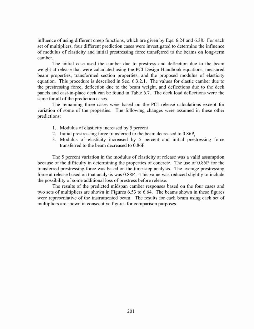
201
influence of using different creep functions, which are given by Eqs. 6.24 and 6.38. For eachset of multipliers, four different prediction cases were investigated to determine the influenceof modulus of elasticity and initial prestressing force transferred to the beams on long-termcamber.
The initial case used the camber due to prestress and deflection due to the beamweight at release that were calculated using the PCI Design Handbook equations, measuredbeam properties, transformed section properties, and the proposed modulus of elasticityequation. This procedure is described in Sec. 6.3.2.1. The values for elastic camber due tothe prestressing force, deflection due to the beam weight, and deflections due to the deckpanels and cast-in-place deck can be found in Table 6.7. The deck load deflections were thesame for all of the prediction cases.
The remaining three cases were based on the PCI release calculations except forvariation of some of the properties. The following changes were assumed in these otherpredictions:
1.� Modulus of elasticity increased by 5 percent2.� Initial prestressing force transferred to the beam decreased to 0.86Pi
3.� Modulus of elasticity increased by 5 percent and initial prestressing forcetransferred to the beam decreased to 0.86Pi
The 5 percent variation in the modulus of elasticity at release was a valid assumptionbecause of the difficulty in determining the properties of concrete. The use of 0.86Pi for thetransferred prestressing force was based on the time-step analysis. The average prestressingforce at release based on that analysis was 0.88Pi. This value was reduced slightly to includethe possibility of some additional loss of prestress before release.
The results of the predicted midspan camber responses based on the four cases andtwo sets of multipliers are shown in Figures 6.53 to 6.64. The beams shown in these figureswere representative of the instrumented beam. The results for each beam using each set ofmultipliers are shown in consecutive figures for comparison purposes.
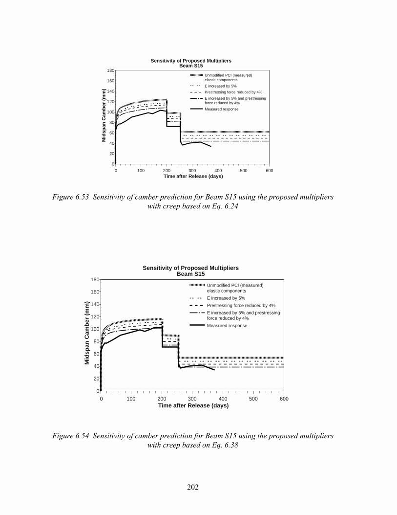
202
180
160
140
120
100
80
60
40
20
0
Mid
span
Cam
ber
(m
m)
0 100 200 300 400 500 600
Sensitivity of Proposed MultipliersBeam S15
Time after Release (days)
Unmodified PCI (measured)elastic components
E increased by 5%
Prestressing force reduced by 4%
E increased by 5% and prestressingforce reduced by 4%
Measured response
Figure 6.53 Sensitivity of camber prediction for Beam S15 using the proposed multiplierswith creep based on Eq. 6.24
180
160
140
120
100
80
60
40
20
0
Mid
span
Cam
ber
(m
m)
0 100 200 300 400 500 600
Sensitivity of Proposed MultipliersBeam S15
Time after Release (days)
Unmodified PCI (measured)elastic components
E increased by 5%
Prestressing force reduced by 4%
E increased by 5% and prestressingforce reduced by 4%
Measured response
Figure 6.54 Sensitivity of camber prediction for Beam S15 using the proposed multiplierswith creep based on Eq. 6.38

203
160
140
120
100
80
60
40
20
0
-20
Mid
span
Cam
ber
(m
m)
0 200 400 600 800 1000 1200
Sensitivity of Proposed MultipliersBeam S25
Time after Release (days)
Unmodified PCI (measured)elastic components
E increased by 5%
Prestressing force reduced by 4%
E increased by 5% and prestressingforce reduced by 4%
Measured response
Figure 6.55 Sensitivity of camber prediction for Beam S25 using the proposed multiplierswith creep based on Eq. 6.24
160
140
120
100
80
60
40
20
0
-20
Mid
span
Cam
ber
(m
m)
0 200 400 600 800 1000 1200
Sensitivity of Proposed MultipliersBeam S25
Time after Release (days)
Unmodified PCI (measured)elastic components
E increased by 5%
Prestressing force reduced by 4%
E increased by 5% and prestressingforce reduced by 4%
Measured response
Figure 6.56 Sensitivity of camber prediction for Beam S25 using the proposed multiplierswith creep based on Eq. 6.38

204
200
180
160
140
120
100
80
60
40
20
0
Mid
span
Cam
ber
(m
m)
0 200 400 600 800 1000 1200
Sensitivity of Proposed MultipliersBeam N21
Time after Release (days)
Unmodified PCI (measured)elastic components
E increased by 5%
Prestressing force reduced by 4%
E increased by 5% and prestressingforce reduced by 4%
Measured response
Figure 6.57 Sensitivity of camber prediction for Beam N21 using the proposed multiplierswith creep based on Eq. 6.24
200
180
160
140
120
100
80
60
40
20
0
Mid
span
Cam
ber
(m
m)
0 200 400 600 800 1000 1200
Sensitivity of Proposed MultipliersBeam N21
Time after Release (days)
Unmodified PCI (measured)elastic components
E increased by 5%
Prestressing force reduced by 4%
E increased by 5% and prestressingforce reduced by 4%
Measured response
Figure 6.58 Sensitivity of camber prediction for Beam N21 using the proposed multiplierswith creep based on Eq. 6.38
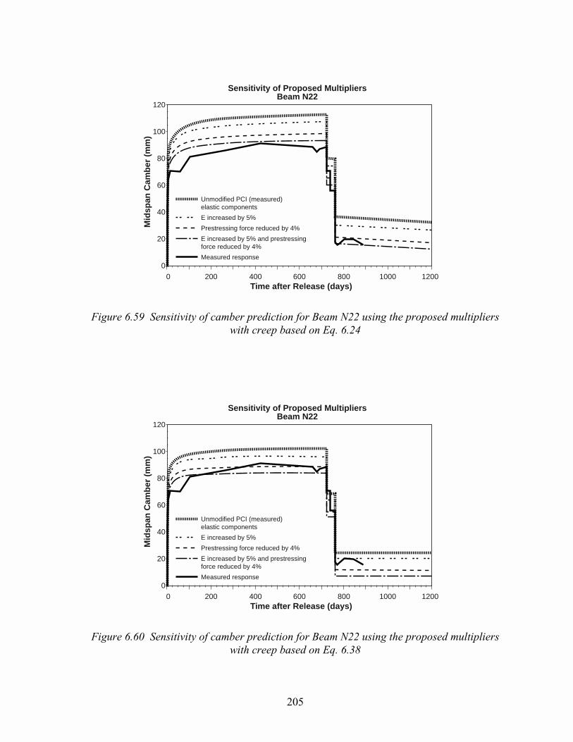
205
120
100
80
60
40
20
0
Mid
span
Cam
ber
(m
m)
0 200 400 600 800 1000 1200
Sensitivity of Proposed MultipliersBeam N22
Time after Release (days)
Unmodified PCI (measured)elastic components
E increased by 5%
Prestressing force reduced by 4%
E increased by 5% and prestressingforce reduced by 4%
Measured response
Figure 6.59 Sensitivity of camber prediction for Beam N22 using the proposed multiplierswith creep based on Eq. 6.24
120
100
80
60
40
20
0
Mid
span
Cam
ber
(m
m)
0 200 400 600 800 1000 1200
Sensitivity of Proposed MultipliersBeam N22
Time after Release (days)
Unmodified PCI (measured)elastic components
E increased by 5%
Prestressing force reduced by 4%
E increased by 5% and prestressingforce reduced by 4%
Measured response
Figure 6.60 Sensitivity of camber prediction for Beam N22 using the proposed multiplierswith creep based on Eq. 6.38

206
180
160
140
120
100
80
60
40
20
0
Mid
span
Cam
ber
(m
m)
0 200 400 600 800 1000 1200
Sensitivity of Proposed MultipliersBeam N31
Time after Release (days)
Unmodified PCI (measured)elastic components
E increased by 5%
Prestressing force reduced by 4%
E increased by 5% and prestressingforce reduced by 4%
Measured response
Figure 6.61 Sensitivity of camber prediction for Beam N31 using the proposed multiplierswith creep based on Eq. 6.24
180
160
140
120
100
80
60
40
20
0
Mid
span
Cam
ber
(m
m)
0 200 400 600 800 1000 1200
Sensitivity of Proposed MultipliersBeam N31
Time after Release (days)
Unmodified PCI (measured)elastic components
E increased by 5%
Prestressing force reduced by 4%
E increased by 5% and prestressingforce reduced by 4%
Measured response
Figure 6.62 Sensitivity of camber prediction for Beam N31 using the proposed multiplierswith creep based on Eq. 6.38

207
180
160
140
120
100
80
60
40
20
0
Mid
span
Cam
ber
(m
m)
0 100 200 300 400 500 600
Sensitivity of Proposed MultipliersBeam N32
Time after Release (days)
Unmodified PCI (measured)elastic components
E increased by 5%
Prestressing force reduced by 4%
E increased by 5% and prestressingforce reduced by 4%
Measured response
Figure 6.63 Sensitivity of camber prediction for Beam N32 using the proposed multiplierswith creep based on Eq. 6.24
180
160
140
120
100
80
60
40
20
0
Mid
span
Cam
ber
(m
m)
0 100 200 300 400 500 600
Sensitivity of Proposed MultipliersBeam N32
Time after Release (days)
Unmodified PCI (measured)elastic components
E increased by 5%
Prestressing force reduced by 4%
E increased by 5% and prestressingforce reduced by 4%
Measured response
Figure 6.64 Sensitivity of camber prediction for Beam N32 using the proposed multiplierswith creep based on Eq. 6.38
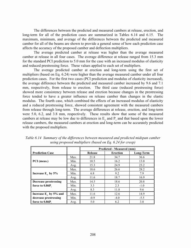
208
The differences between the predicted and measured cambers at release, erection, andlong-term for all of the prediction cases are summarized in Tables 6.14 and 6.15. Themaximum, minimum, and average of the differences between the predicted and measuredcamber for all of the beams are shown to provide a general sense of how each prediction caseaffects the accuracy of the proposed camber and deflection multipliers.
The average predicted camber at release was higher than the average measuredcamber at release in all four cases. The average difference at release ranged from 15.3 mmfor the standard PCI prediction to 5.0 mm for the case with an increased modulus of elasticityand reduced prestressing force. These values applied to each set of multipliers.
The average predicted camber at erection and long-term using the first set ofmultipliers (based on Eq. 6.24) were higher than the average measured camber under all fourprediction cases. For the first two cases (PCI prediction and modulus of elasticity increased),the average difference between the predicted and measured camber increased by 9.6 and 7.1mm, respectively, from release to erection. The third case (reduced prestressing force)showed more consistency between release and erection because changes in the prestressingforce tended to have a greater influence on release camber than changes in the elasticmodulus. The fourth case, which combined the effects of an increased modulus of elasticityand a reduced prestressing force, showed consistent agreement with the measured cambersfrom release through long-term. The average differences at release, erection, and long-termwere 5.0, 6.2, and 3.8 mm, respectively. These results show that some of the measuredcambers at release may be low due to differences in Eci and Po and that based upon the lowerrelease cambers, the measured cambers at erection and long-term can be accurately predictedwith the proposed multipliers.
Table 6.14 Summary of the differences between measured and predicted midspan camberusing proposed multipliers (based on Eq. 6.24 for creep)
Predicted - Measured (mm)Prediction Case Release Erection Long-Term
Max. 21.8 34.7 36.6PCI (meas.) Min. 10.5 16.2 13.0
Avg. 15.3 24.9 23.2Max. 18.6 26.6 28.2
Increase Eci by 5% Min. 6.8 9.2 7.9Avg. 11.6 18.7 16.9
Decrease prestressing Max. 14.5 18.6 20.8force to 0.86Pi Min. 3.3 2.3 -1.0
Avg. 8.3 11.8 9.6Increase Eci by 5% and Max. 11.6 12.6 14.9decrease prestressing Min. -0.9 -4.0 -5.5force to 0.86Pi Avg. 5.0 6.2 3.8

209
Table 6.15 Summary of the differences between measured and predicted midspan camberusing proposed multipliers (based on Eq. 6.38 for creep)
Predicted - Measured (mm)Prediction Case Release Erection Long-Term
Max. 21.8 20.5 23.9PCI (meas.) Min. 10.5 3.8 6.0
Avg. 15.3 14.1 14.6Max. 18.6 14.8 18.1
Increase Eci by 5% Min. 6.8 -2.7 -0.5Avg. 11.6 8.4 8.8
Decrease prestressing Max. 14.5 10.9 14.1force to 0.86Pi Min. 3.3 -9.1 -7.0
Avg. 8.3 1.9 2.1Increase Eci by 5% and Max. 11.6 5.7 8.8decrease prestressing Min. -0.9 -14.9 -12.9force to 0.86Pi Avg. 5.0 -3.2 -3.0
The average predicted cambers at erection and long-term using the second set ofmultipliers (based on Eq. 6.38) were higher than the average measured camber for all of theprediction cases except the last one. For the unmodified PCI prediction, the averagedifferences between the predicted and measured camber at release and erection were nearlyidentical. The average differences at release, erection, and long-term were 15.3, 14.1, and14.6 mm, respectively. The other three prediction cases showed a reduction in the averagedifferences from release to erection. The average differences for the fourth prediction caseshowed a change from 5.0 mm at release to -3.0 mm at erection.
Both sets of multipliers showed consistency between the differences at erection and atrelease. Errors in the prediction models between release and erection were not magnifiedbecause the composite U-beam section was extremely stiff and because the deck loads wereplaced at a late age. In addition, a majority of the creep for the high performance concrete U-beams occurred within the first 100 days. If future construction schedules using the HPC U-beams are on the order of 50 to 75 days between release and placement of the deck loads, thebeams will probably not show significant additional deflection due to creep.
Based on the results of the presented in Figures 6.53 to 6.64 and in Tables 6.14 and6.15, the prediction of long-term camber and deflection is sensitive to variations in therelease camber as well as the variations in the assumed creep function used to model thebeams. By altering the modulus of elasticity and the initial prestressing force slightly, theproposed multipliers (based on Eq. 6.24) showed very accurate prediction of the measuredmidspan cambers from release to erection.
The second set of multipliers (based on Eq. 6.38) showed less accurate prediction ofcamber growth from release to erection. If the second set of multipliers were assumed to be abetter representation of the camber growth during storage, then there would have to be anadditional source of deflection at release which would cause an offset between the predictions

210
and measurements throughout the life of the beam. This pattern was evident in the PCIprediction case shown in Table 6.15. A possible source of this offset may be due to early-agetemperature gradients. However, it is more likely that the ultimate creep coefficient for thesecond set of multipliers was probably an underestimate for the U-beams.
In considering the sensitivity analysis using both sets of multipliers and all fourprediction cases, differences between the predicted and measured cambers at release anderection are caused by the inability to precisely model the actual behavior of prestressedconcrete beams in the field. Small differences in material properties, prestressing force, andthe estimation of thermally induced movements can have a remarkable effect on the accuracyof predictions. In addition, errors in measurement techniques contribute to these differences.The proposed multipliers that were based on the time-step analysis and Eq. 6.24 for creep ofthe concrete provide a reasonable estimate of long-term behavior of prestressed highperformance concrete U-beams with spans ranging from 35 to 42 meters.

211
CHAPTER 7. SUMMARY, CONCLUSIONS, AND RECOMMENDATIONS
7.1 SUMMARY
Twelve full-scale prestressed high performance concrete Texas Type U54 bridgebeams with span lengths ranging from 35.55 to 41.25 meters were instrumented andmonitored in the field. The instrumented U-beams were fabricated using 15.2 mm-diameterlow-relaxation prestressing strands and concrete with design compressive strengths between80.0 and 90.3 MPa. Time-dependent camber, deflection, strain at the center of gravity of theprestressing strands, and strain distributions at midspan were measured from transfer of theprestressing force until five months after completion of the composite deck. Internal beamtemperatures at midspan were also measured during that time period, allowing for themeasurement of temperature gradients over the beam depth. Monitoring of deformationbehavior in the bridge will continue for several more years. Companion tests were performedto determine the time-dependent material properties of the high performance concrete used tofabricate the instrumented beams.
The measured time-dependent camber, deflection, and prestress losses at midspanwere compared to results obtained using AASHTO and PCI prediction techniques.Predictions were also made using an analytical time-step method that was developed on acomputer spreadsheet program by the author. The analytical time-step method used themeasured time-dependent material properties for the beams. The analytical time-step methodpredicted the time-dependent camber, deflection, and prestress losses in the instrumentedbeams the most accurately.
A set of camber and deflection multipliers were developed based on the analyticaltime-step method and the measured prestress losses and material properties for theinstrumented beams. The equations for these multipliers were well-suited for programmingon a computer, although they could also be used for hand calculations.
A second set of camber and deflection multipliers were developed based on analternative curve fit to the measured creep data for the U-beam specimens. Both sets ofmultipliers were used to perform a sensitivity analysis on the prediction of long-term camberand deflection behavior. The creep function, the modulus of elasticity at release, andprestressing force transferred to the beams were varied to determine how differentcombinations of these three variables affected long-term camber of the instrumented U-beams. The different predictions were compared to the measured camber and deflectionresponses for several representative beams.
7.2 CONCLUSIONS
The conclusions presented in this section are based on the field instrumentationprocedures, the measured behavior of the beams, the results of the companion tests, and theresults of the analytical techniques for predicting long-term behavior. Conclusions thatspecify quantities or expressions for time-dependent behavior should only be considered

212
valid for Texas Type U54 beams that are fabricated using a similar high performanceconcrete mix and that have span lengths in the range of 35 and 42 meters.
The following conclusions are based upon the results of the field instrumentation ofthe U-beams and composite deck:
1.� Coordination of efforts between the researchers and the contractors was anessential aspect of this field instrumentation study. Lack of propercommunication resulted in missed readings and damaged instrumentation.Fortunately, the overall experience was very good in this study and goodcoordination was generally achieved.
2.� The tensioned piano wire camber and deflection measuring system worked welland allowed for very precise measurement. However, the steel ruler at midspanwas susceptible to being disrupted during storage and during transportation of thebeams. Since this system depended upon an initial reference measurement,disruption of the ruler was a critical problem. A more permanent means ofattaching the ruler to the beam should be used in the future to avoid possiblemovement of the ruler.
3.� The precise surveying system that was used for measuring camber and deflectionof the beams after they were erected in the bridge worked well and had acceptableaccuracy and repeatability. In addition, this system was an efficient method ofmeasuring camber and deflection at the various stages of construction as thebridge was completed. A set of measurements for all twelve beams generallyrequired one hour to complete.
4.� The nylon cable ties did not adequately hold the strain gages that were placed inthe cast-in-place deck in their intended positions. The various aspects of the deckcasting operation, including pouring of the concrete over the gages, tended tomove the deck gages with relative ease.
5.� Measurement of surface strains using the Demec mechanical gages required themeasurement of surface temperatures at the times of the readings. The lack ofsurface temperature data rendered the surface strain measurements relativelyuseless for long-term measurements.
6.� The bonded electrical resistance strain gages (ERSGs) that were embedded in thebeam provided quality data for an average of 150 days after release. ERSGs werenot reliable measurement tools for long-term strain behavior in these fieldinstrumented U-beams.
7.� The embedded vibrating wire (VW) gages generally provided quality short andlong-term strain data. Although VW gages were quite costly, they were verydurable and required very little preparation and installation time. Several VWgages are providing valid strain measurements over 900 days after release.
The following conclusions are based on the measured behavior of the beams, theresults of the companion tests, and the results of the analytical time-step method forpredicting time-dependent camber, deflection, and prestress losses:

213
1.� The AASHTO formula for modulus of elasticity should not be used for theprediction of long-term behavior for the high performance concrete U-beams inthis study. Equation 5.2, which is given in Sec. 5.2.2, should be used to calculatethe modulus of elasticity for the beam concrete in this study and for other concretecontaining limestone aggregate and having compressive strengths greater than 60MPa.
2.� Creep strains were less than those predicted by expressions recommended by ACICommittee 209 for normal strength concrete. The prediction of creep deformationfor beams made with the high performance concrete mix used in this study shouldbe based on Eq. 5.3 in Sec. 5.2.3.
3.� Shrinkage strains were less than those predicted by expressions recommended byACI Committee 209 for normal strength concrete. The prediction of shrinkagestrain for beams made with the high performance concrete mix used in this studyshould be based on Eq. 5.6 in Sec. 5.2.3.
4.� Temperature gradients were nonlinear in the noncomposite U-beam section andwere highly nonlinear in the composite U-beam section. The maximumtemperature gradient observed over the depth of the composite U-beams betweenNovember of 1996 and March of 1997 was 12 �C.
5.� Temperature gradients on sunny days can cause thermal movements of at least 12mm in the noncomposite U-beams and at least 8 mm in the composite U-beams.
6.� Prediction of midspan camber immediately after release was sensitive to themodulus of elasticity and prestressing force used in the calculations. This isillustrated in Sec. 6.5.2.
7.� The assumption of four percent prestress losses before release due to shrinkage,relaxation, and an increase in strand temperature after stressing should be used asan estimation of prestress losses before release. In lieu of an exact analysis forelastic shortening, the initial elastic camber for U-beams with low-relaxationstrands should be calculated using 0.88 as the ratio of prestressing forceimmediately after release to the initial force.
8.� The AASHTO method for predicting prestress losses using design propertiesoverestimated the measured prestress losses by an average of 8 percent. TheAASHTO method should not be used for predicting prestress losses for highperformance concrete U-beams similar to those in this study.
9.� The analytical time-step method predicted the prestress losses for the U-beamswith acceptable accuracy, overestimating the actual prestress losses by an averageof only 1.5 percent. This is shown in Sec. 6.4.2.2.
10.�The proposed multipliers for predicting camber and deflection based on Eq. 6.24for creep, which are developed in Sec. 6.5.1, predicted the measured camber anddeflection of the U-beams with reasonable accuracy.
11.�The time-dependent midspan cambers (or deflections) of the U-beams predictedusing the proposed multipliers were sensitive to the creep coefficient function, the

214
modulus of elasticity at release, and the initial prestressing force transferred to thebeams. This is shown in Sec. 6.5.2.
12.�The long-term deflection of the U-beams due to the superimposed deck load isprojected to be very small because the composite section was nearly three times asstiff as the noncomposite section and because a majority of the ultimate creepdeformation occurred during storage.
13.�Uneven cooling of the beam cross section, which occurred after the forms werestripped, may cause a thermally induced component of deflection in the beam thatbecomes evident just after release. Based on limited temperature data duringcasting, the magnitude of this deflection may be as large as 12 mm.
14.�The proper correction for camber or deflection induced by temperature gradientsmay be in reference to a nonuniform temperature gradient in the beam before theforms are stripped rather than a uniform temperature gradient of 20 �C, which wasused for the beams in this study.
15.�Strain measurements at release in the bottom flange of the U-beams may havebeen artificially high due to restraint offered by the prestressing bed to the beamsas they tried to shorten due to cooling and shrinkage. Upon release, the restraintwould be removed and an additional compressive strain would be measured by thestrain gages.
7.3 RECOMMENDATIONS
1.� The precise surveying system for measuring beam camber and deflection after thebeams were erected in the bridge, which is described in Sec. 3.3.5, was veryefficient and should be used in future projects. It should also be considered foruse while the beams are in storage.
2.� The vibrating wire strain gages should be used more extensively in fieldinstrumentation projects because of their durability, ease of preparation andinstallation, and quality of long-term results. The ability to obtain long-termstrain data is essential for determining prestress loss behavior in high performanceconcrete bridge beams.
3.� The proposed multipliers (based on Eq. 6.24) should be used to estimate camberand deflection for long-span U-beams made with high strength concrete mixessimilar to the one used for the U-beams in this study.
4.� Creep and shrinkage tests should be performed on other high performanceconcrete beam mixes to gain further knowledge of the deformation properties ofconcretes with very high strength that are used in prestressing applications.

215
REFERENCES
1. Ralls, M. L., Ybanez, L., and Panak, J. J., “The New Texas U-Beam Bridges: AnAesthetic and Economical Design Solution,” PCI Journal, Vol. 38, No. 5, Sept.–Oct.1993, pp. 20-29.
2. Peterman, M. B., and Carrasquillo, R. L., “Production of High Strength Concrete,”Research Report 315-1F, Center for Transportation Research, The University ofTexas at Austin, October 1983.
3. Russell, B. W., “Impact of High Strength Concrete on the Design and Construction ofPretensioned Girder Bridges,” PCI Journal, Vol. 39, No. 4, July–Aug. 1994, pp. 76-89.
4. Goodspeed, C. H., Vanikar, S., and Cook, R. A., “High-Performance ConcreteDefined for Highway Structures,” Concrete International, Vol. 18, No. 2, February1996, pp. 62–67.
5. Cetin, A., and Carrasquillo, R. L., “Effect of Accelerated Heat Curing and MixCharacteristics on the Heat Development and Mechanical Properties of HighPerformance Concrete,” Research Report 580-4 (Preliminary Review Copy), Centerfor Transportation Research, The University of Texas at Austin, December 1995.
6. Barrios, A. O., Burns, N. H., and Carrasquillo, R. L., “Behavior of High StrengthConcrete Pretensioned Girders During Transfer of Prestressing Forces,” ResearchReport 580-2 (Preliminary Review Copy), Center for Transportation Research, TheUniversity of Texas at Austin, May 1994.
7. Carlton, M. P. and Carrasquillo, R. L., “Quality Control of High PerformanceConcrete for Highway Bridges,” Research Report 580-3 (Preliminary Review Copy),Center for Transportation Research, The University of Texas at Austin, June 1995.
8. Farrington, E. W., Burns, N. H., and Carrasquillo, R. L., “Creep and Shrinkage ofHigh Performance Concrete,” Research Report 580-5 (Preliminary Review Copy),Center for Transportation Research, The University of Texas at Austin, February1996.
9. Durning, T. A., and Rear, K.B., “Braker Lane Bridge: High Strength Concrete inPrestressed Bridge Girders,” PCI Journal, Vol. 83, No. 3, May–June 1993, pp. 46-51.
10. Castrodale, R. W., Kreger, M. E., and Burns, N. H., “A Study of Pretensioned HighStrength Concrete Girders in Composite Highway Bridges — DesignConsiderations,” Research Report 381-4F, Center for Transportation Research, TheUniversity of Texas at Austin, January 1988.
216
11. Castrodale, R. W., Kreger, M. E., and Burns, N. H., “A Study of Pretensioned HighStrength Concrete Girders in Composite Highway Bridges — Laboratory Tests,”Research Report 381-3, Center for Transportation Research, The University of Texasat Austin, January 1988.
12. Carrasquillo, P. M. and Carrasquillo, R. L., “Guidelines for Use of High StrengthConcrete in Texas Highways,” Research Report 367-1F, Center for TransportationResearch, The University of Texas at Austin, August 1986.
13. American Concrete Institute Committee 363, “State-of-the-Art Report on HighStrength Concrete,” ACI Journal, Proceedings, Vol. 81, No. 4, July–Aug. 1984, pp.364–411.
14. Lin, T. Y., and Burns, N. H., Design of Prestressed Concrete Structures, ThirdEdition, John Wiley and Sons, New York, New York, 1981, 646 pp.
15. Carrasquillo, R. L., Nilson, A. H., and Slate, F. O., “Properties of High StrengthConcrete Subject to Short-Term Loads,” ACI Journal, Proceedings, Vol. 78, No. 3,May–June 1981, pp. 171–178.
16. American Association of State Highway and Transportation Officials, StandardSpecifications for Highway Bridges, Fifteenth Edition, Washington, D.C., 1992.
17. American Concrete Institute, Building Code Requirements for Structural Concrete(ACI 318-95) and Commentary (ACI 318R-95), Detroit, 369 pp.
18. Libby, J. R., Modern Prestressed Concrete: Design Principles and ConstructionMethods, Fourth Edition, Van Nostrand Reinhold, New York, New York, 871 pp.
19. American Concrete Institute Committee 209, “Prediction of Creep, Shrinkage, andTemperature Effects in Concrete Structures,” Designing for Creep and Shrinkage inConcrete Structures, SP-76, American Concrete Institute, Detroit, 1982, pp. 193–300.
20. Ngab, A. S., Nilson, A. H., and Slate, F. O., “Shrinkage and Creep of High StrengthConcrete,” ACI Journal, Proceedings, Vol. 78, No. 4, July–Aug. 1981, pp. 255–261.
21. American Concrete Institute Committee 517, “Low Pressure Steam Curing,” ACIReport Title No. 60-48, American Concrete Institute, Detroit, 1963.
22. Hanson, J. A., “Prestress Loss as Affected by Type of Curing,” PCI Journal, Vol. 9,No. 2, April 1964, pp. 69–93.
23. Swamy, R. N., and Anand, K. L., “Shrinkage and Creep Properties of High StrengthStructural Concrete,” Civil Engineering and Public Works Review (London), Vol. 68,No. 80, October 1973, pp. 859–868.
217
24. Arrelaga, J. A., “Instrumentation Systems for Post-Tensioned Segmental Box GirderBridges,” unpublished master’s thesis, The University of Texas at Austin, Dec. 1991.
25. Russell, H. G., Implementation Program on High Performance Concrete-Guidelinesfor Instrumentation of Bridges, Report to FHWA, February 1996.
26. Kelly, D. J., Bradberry, T. E., and Breen, J. E., “Time Dependent Deflections ofPretensioned Beams,” Research Report 381-1, Center for Transportation Research,The University of Texas at Austin, August 1987.
27. Precast/Prestressed Concrete Institute, PCI Design Handbook: Precast andPrestressed Concrete, Fourth Edition, Chicago, 1992.
28. Martin, L. D., “A Rational Method for Estimating Camber and Deflection of PrecastPrestressed Concrete Members,” PCI Journal, Vol. 22, No. 1, Jan.–Feb. 1977, pp.100–108.
29. Suttikan, C., “A Generalized Solution for Time-Dependent Response and Strength ofNoncomposite and Composite Prestressed Concrete Beams,” unpublished doctoraldissertation, The University of Texas at Austin, Aug. 1978.
30. Rao, V. J., and Dilger, W. H., “Time-Dependent Deflections of CompositePrestressed Concrete Beams,” Deflection of Concrete Structures, SP-43, AmericanConcrete Institute, Detroit, 1974.
31. Corley, W. G., Sozen, M. A., and Seiss, C. P., “Time-Dependent Deflections ofPrestressed Concrete Beams,” Bulletin No. 307, Highway Research Board,Washington, D.C., 1961.
32. Furr, H. L., and Sinno, R., “Creep in Prestressed Lightweight Concrete,” ResearchReport 69-2, Study 2-5-63-69, Texas Transportation Institute, Texas A&M UniversitySystem, College Station, Texas, Oct. 1967.
33. Furr, H. L., Sinno, R., and Ingram L.L., “Prestress Loss and Creep Camber in aHighway Bridge with Reinforced Concrete Slab on Pretensioned Prestressed ConcreteBeams,” Research Report 69-3 (Final), Study 2-5-63-69, Texas TransportationInstitute, Texas A&M University System, College Station, Texas, Oct. 1968.
34. Branson, D. E., Meyers, B. L., and Kripanarayanan, K. M., “Loss of Prestress,Camber and Deflection of Noncomposite and Composite Structures Using DifferentWeight Concretes,” Iowa Highway Commission Final Report, No. 70-6, Aug. 1970.
35. Gamble, W. L., “Field Investigation of a Continuous Composite Prestressed I-BeamHighway Bridge Located in Jefferson County, Illinois,” Structural Research Series
218
No. 360, Civil Engineering Studies, University of Illinois at Urbana-Champaign,Urbana, June 1970.
36. Houseshell, D. M., Anderson, T. C., and Gamble, W. L., “Field Investigation of aPrestressed Concrete Highway Bridge Located in Douglas County, Illinois,”Structural Research Series No. 375, Civil Engineering Studies, University of Illinoisat Urbana-Champaign, Urbana, Feb. 1972.
37. Gamble, W. L., “Long-Term Behavior of a Prestressed I-Girder Highway Bridge inChampaign County, Illinois,” Structural Research Series No. 470, Civil EngineeringStudies, University of Illinois at Urbana-Champaign, Urbana, Dec. 1979.
38. Zia, P., Preston, H. K., Scott, N. L., and Workman, E. B. “Estimating PrestressLosses,” Concrete International, Vol. 1, No. 6, June 1979, pp. 32–38.
39. PCI Committee on Prestress Losses, “Recommendations for Estimating PrestressLosses,” PCI Journal, Vol. 20, No. 4, July–Aug. 1975, pp. 43–75.
40. Subcommittee 5, ACI Committee 435, “Deflections of Prestressed ConcreteMembers,” ACI Journal, Proceedings, Vol. 60, No. 12, Dec. 1963, pp. 1697–1728.
41. Tadros, M. K., Ghali, A., and Dilger, W. H., “Time-Dependent Prestress Loss andDeflection in Prestressed Concrete Members,” PCI Journal, Vol. 20, No. 3, May–June 1975, pp. 86–98.
42. Tadros, M. K., Ghali, A., and Meyer, A. W., “Prestress Loss and Deflection ofPrestressed Concrete Members,” PCI Journal, Vol. 30, No. 1, Jan.–Feb. 1985, pp.114–141.
43. Branson, D. E., and Kripanarayanan, K. M., “Loss of Prestress, Camber andDeflection of Non-composite and Composite Prestressed Concrete Structures,” PCIJournal, Vol. 16, No. 5, Sept.–Oct. 1971, pp. 22–52.
44. Sinno, R., and Furr, H. L., “Computer Program for Predicting Prestress Loss andCamber,” PCI Journal, Vol. 17, No. 5, Sept.–Oct. 1972.
45. Hernandez, H. D., and Gamble, W. L., “Time-dependent Prestress Losses inPretensioned Concrete Construction,” Structural Research Series N. 417, CivilEngineering Studies, University of Illinois at Urbana-Champaign, Urbana, 1975.
46. Grouni, H. N., “Prestressed Concrete: A Simplified Method for Loss Computation,”ACI Journal, Proceedings, Vol. 70, No. 2, Feb. 1973, pp. 15–29.
47. Huang, T., “Study of Prestress Losses Conducted by Lehigh University,” PCIJournal, Vol. 27, No. 5, Sept.–Oct. 1982, pp. 48–61.
219
48. Ingram, L. L., and Butler, H. D., “Prestressed Concrete Bridge Girder DesignProgram,” Research Report 149-1 (Final), Texas Transportation Institute, TexasA&M University System, College Station, Texas, Nov. 1970.
49. Texas State Department of Highways and Public Transportation Bridge Division,Prestressed Concrete Beam Design/Analysis Program User Guide, PSTRS14, March1990.
50. American Society for Testing and Materials, “Standard Test Method for StaticModulus of Elasticity and Poisson’s Ratio of Concrete in Compression,” ASTMC469-87, Philadelphia, 1987.
51. American Society for Testing and Materials, “Standard Test Method for CompressiveStrength of Cylindrical Concrete Specimens,” ASTM C-39-86, Philadelphia, 1986.
52. American Society for Testing and Materials, “Standard Test Method for Creep ofConcrete in Compression,” ASTM C512-87, Philadelphia, 1987.
53. Priestly, M. N. J., “Design of Concrete Bridges for Temperature Gradients,” ACIJournal, Proceedings, V. 75, No. 5, May 1978, pp. 209–217.
54. Potgieter, I. C., and Gamble, W. L., “Nonlinear Temperature Distributions in Bridgesat Different Locations in the United States,” PCI Journal, V. 34, No. 4, July–August1989, pp. 80–103.
55. Radolli, M., and Green, R., “Thermal Stresses in Concrete Bridge SuperstructuresUnder Summer Conditions,” Transportation Research Record, No. 547,Transportation Research Board, 1975, pp. 23–36.
56. Committee on Prestress Losses, “Recommendations for Estimating Prestress Losses,”PCI Journal, Vol. 20, No. 4, July–Aug. 1975, pp. 43–75.

220

221
APPENDIX A:
DEBONDING DETAILS

222

223
Table A1 Debonding details for instrumented beams in the southbound main lanes bridge
Debonded Strands and Length from End of Beam2 (m)
Beam Row Total1 0.91 1.83 2.74 3.66 4.57 5.49 6.40 8.23 9.14
S14 1 20 7,9 3,5 10,12 8 --- 6 4 2 ---
2 4 3,5 --- --- --- --- --- --- --- ---
S15 1 20 7,9 3,5 10,12 8 --- 6 4 2 ---
2 4 3,5 --- --- --- --- --- --- --- ---
S16 1 20 9 3,5,7 8,10,12 4,6 2 --- --- --- ---
2 6 3,5,7 --- --- --- --- --- --- --- ---
S24 1 20 9 3,5,7 8,10,12 4,6 2 --- --- --- ---
2 6 3,5,7 --- --- --- --- --- --- --- ---
S25 1 20 9 3,5,7 8,10,12 4,6 2 --- --- --- ---
2 6 3,5,7 --- --- --- --- --- --- --- ---
S26 1 20 --- 7,9 3,5 12 10 8 6 4 2
2 14 4,7,9,11,13 3,5 --- --- --- --- --- --- ---
Notes:
1.� Total number of strands debonded in each row at each end of the beam.
2.� Numbers correspond to the strand designations defined in Fig. A.1. Debonded strands appear in the
column that corresponds to the length from the end of the beam that the debonding was applied.

224
Table A2 Debonding details for instrumented beams in the northbound main lanes bridge
Debonded Strands and Length from End of Beam2 (m)
Beam Row Total1 0.91 1.83 2.74 3.66 4.57 5.49 6.40 8.23 9.14
N21 1 20 --- 7,9 3,5 12 10 8 6 4 2
2 14 4,7,9,11,13 3,5 --- --- --- --- --- --- ---
N22 1 20 9 3,5,7 8,10,12 4,6 2 --- --- --- ---
2 6 3,5,7 --- --- --- --- --- --- --- ---
N23 1 20 9 3,5,7 8,10,12 4,6 2 --- --- --- ---
2 6 3,5,7 --- --- --- --- --- --- --- ---
N31 1 20 --- 3,5,7 9,12 8,10 6 4 2 --- ---
2 12 5,7,9,11,13 3 --- --- --- --- --- --- ---
N32 1 20 7,9 3,5 10,12 8 --- 6 4 2 ---
2 4 3,5 --- --- --- --- --- --- --- ---
N33 1 20 7,9 3,5 10,12 8 --- 6 4 2 ---
2 4 3,5 --- --- --- --- --- --- --- ---
Notes:
1.� Total number of strands debonded in each row at each end of the beam.
2.� Numbers correspond to the strand designations defined in Fig. A.1. Debonded strands appear in the
column that corresponds to the length from the end of the beam that the debonding was applied.
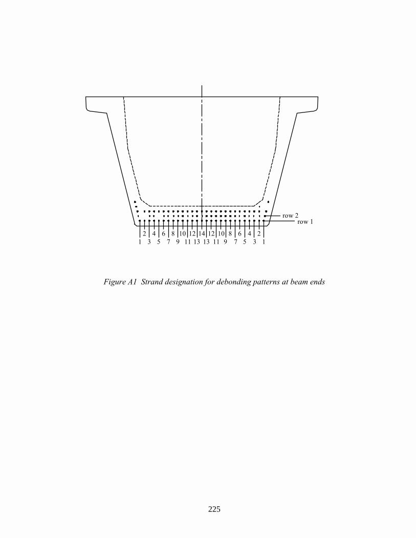
225
�����
�����
�� � �� � ���� �� ��
� �� ��� �� ���� ����
Figure A1 Strand designation for debonding patterns at beam ends