Time Domain BEM: Numerical Aspectsof Collocation and Galerkin Formulations

Martin Schanz, Thomas Ruberg and Lars Kielhorn

Abstract Time domain Boundary Element formulations are very well suited to treatwave propagation phenomena in semi-infinte domains, e.g., to simulate phenom-ena in earthquake engineering. Beside an analytical integration within each timestep there is the formulation based on the Convolution Quadrature Method whichutilizes the Laplace domain fundamental solutions. Within this technique not onlythe extension to inelastic material behavior is easy also the formulation of a sym-metric Galerkin procedure can be established because the regularisation has to beperformed only for the Laplace domain kernels.

Here, a collocation method is presented resulting in a saddle point formulationas well as a symmetric Galerkin procedure. Both techniques are numerically com-pared also with the usual collocation formulation. Both new formulations show abetter numerical behavior, i.e., the condition numbers of the respective matrices areimproved. This yields also to a better stability in time.

1 Introduction

The Boundary Element Method (BEM) in time domain is especially important totreat wave propagation problems in semi-infinite domains. In this application themain advantage of this method becomes obvious, i.e., its ability to model the Som-merfeld radiation condition correctly. Certainly this is not the only advantage ofa time domain BEM but very often the main motivation as, e.g., in earthquakeengineering.

The first boundary integral formulation for elastodynamics was published byCruse and Rizzo (1968). This formulation performs in Laplace domain with a sub-sequent inverse transformation to the time domain to achieve results for the transientbehavior. The corresponding formulation in Fourier domain, i.e., frequency domain,was presented by Domınguez (1978). The first boundary element formulationdirectly in the time domain was developed by Mansur for the scalar wave equation

M. Schanz (B)Institute of Applied Mechanics, Graz University of Technology, Austriae-mail: m.schanz@tugraz.at

G.D. Manolis, D. Polyzos (eds.), Recent Advances in Boundary Element Methods,DOI 10.1007/978-1-4020-9710-2 27, C© Springer Science+Business Media B.V. 2009

415

416 M. Schanz et al.

and for elastodynamics with zero initial conditions (Mansur, 1983). The extensionof this formulation to non-zero initial conditions was presented by Antes (1985).Detailed information about this procedure may be found in the book of Domınguez(1993). A comparative study of these possibilities to treat elastodynamic problemswith BEM is given by Manolis (1983). A completely different approach to han-dle dynamic problems utilizing static fundamental solutions is the so-called dualreciprocity BEM. This method was introduced by Nardini and Brebbia (1982) anddetails may be found in the monograph of Partridge et al. (1992). A very detailedreview on elastodynamic boundary element formulations and a list of applicationscan be found in two articles of Beskos (1987, 1997).

The above listed methodologies to treat elastodynamic problems with the BEMshow mainly the two ways: direct in time domain or via an inverse transformationin Laplace domain. Mostly, the latter is used, e.g., (Ahmad and Manolis, 1987).Since all numerical inversion formulas depend on a proper choice of their param-eters (Narayanan and Beskos, 1982), a direct evaluation in time domain seems tobe preferable. Also, it is more natural to work in the real time domain and observethe phenomenon as it evolves. But, as all time-stepping procedures, such a formu-lation requires an adequate choice of the time step size. An improper chosen timestep size leads to instabilities or numerical damping. Four procedures to improvethe stability of the classical dynamic time-stepping BE formulation can be quoted:the first employs modified numerical time marching procedures, e.g., Antes andJager (1995) for acoustics, Peirce and Siebrits (1997) for elastodynamics; the sec-ond employs a modified fundamental solution, e.g., Rizos and Karabalis (1994)for elastodynamics; the third employs an additional integral equation for veloci-ties (Mansur et al., 1998); and the last uses weighting methods, e.g., Yu et al. (1998)for elastodynamics and Yu et al. (2000) for acoustics.

Beside these improved approaches there exist the possibility to solve the con-volution integral in the boundary integral equation with the so-called ConvolutionQuadrature Method (CQM) proposed by Lubich (1988). It utilizes the Laplacedomain fundamental solution and results not only in a more stable time steppingprocedure but also damping effects in case of visco- or poroelasticity can be takeninto account (see Schanz and Antes (1997) or Schanz (2001b)). This methodologyis used in the following to establish a collocation based BEM. Different to the usualcollocation methods, here, a saddle point formulation is proposed.

Additionally, a symmetric Galerkin formulation in time domain is presented. ForGalerkin type BE formulations see the overview given by Bonnet et al. (1998).Mostly, those formulations are established for elastostatics. In elastodynamics inLaplace domain Frangi and Novati (1998) have published a symmetric Galerkin for-mulation in 2D. Here, the time domain formulation based on the CQM is presentedfor 3D acoustics and elastodynamics utilizing the advantage that the Laplace domainfundamental solutions can be used and, therefore, the regularisation is much moresimple compared to a pure time domain approach. Finally, only a weakly singularformulation is achieved. A numerical comparison of both proposed time domainformulations with the classical collocation approach closes the paper.

Time Domain BEM 417

Throughout this chapter vectors and tensors are denoted by bold symbols andmatrices by sans serif and upright symbols. An empty space in a matrix is used toavoid writing tedious zeros.

2 Time Domain Boundary Integral Equations

The hyperbolic partial differential equations to be considered in this work are thescalar wave equation and the elastodynamic system. The former is given by

�2 p

�t2(x, t) − c2(Δp)(x, t) = 0 (1)

and describes, for instance, the changes in the acoustic pressure p(x, t) in an ideal-ized fluid. x and t are the position in the three-dimensional Euclidean space R

3 andthe time point from the interval (0,∞). In equation (1), c denotes the speed of wavepropagation, i.e., c2 = κ/ρ with the compressibility κ and the mass density ρ of thefluid.

The dynamic variation of the displacement field u(x, t) of an elastic solid underthe assumptions of linear elasticity is governed by the system of equations

�2u�t2

(x, t) − c21∇(∇ · u(x, t)) + c2

2∇ × (∇ × u(x, t)) = 0 . (2)

The material properties of the solid are represented by c1 and c2, which are thespeeds of propagation of the pressure and the shear waves, respectively. Thesespeeds are given by c2

1 = (λ + μ)/ρ and c22 = μ/ρ with the Lame parameters

λ and μ.

2.1 Hyperbolic Initial Boundary Value Problem

In order to unify the notation, equations (1) and (2) are represented by

ρ�2u

�t2(x, t) + (Lu)(x, t) = 0, (3)

where L is an elliptic partial differential operator. u is now a general unknown func-tion replacing either the acoustic pressure p or the displacement field u. Note thatequation (3) has been obtained by multiplying either (1) or (2) by the mass density ρ.

418 M. Schanz et al.

Using this notation, the considered hyperbolic initial boundary value problemsare of the form

[(ρ

�2

�t2+ L

)u

](x, t) = 0 (x, t) ∈ Ω × (0,∞)

u(y, t) = gD(y, t) (y, t) ∈ ΓD × (0,∞)

q(y, t) = gN (y, t) (y, t) ∈ ΓN × (0,∞)

u(x, t) = 0 (x, t) ∈ Ω × (−∞, 0] .

(4)

The first statement in (4) requires the fulfillment of the partial differential equationin the spatial domain Ω for all times 0 < t < ∞. This spatial domain Ω hasthe boundary Γ which is subdivided into two disjoint sets ΓD and ΓN at whichboundary conditions are prescribed. The Dirichlet boundary condition is the secondstatement of (4) and assigns a given datum gD to the unknown u on the part ΓD ofthe boundary. Similarly, the Neumann boundary condition is the third statement inwhich the datum gN is assigned to the function q on the boundary part ΓN . This newfunction q represents either the acoustic flux qn or the surface traction t dependingon the case of the scalar wave equation (1) or the elastodynamic system (2) as theunderlying model. These quantities can be expressed by

qn(y, t) = limΩ�x→y∈Γ

[∇ p(x, t) · n(y)

](5a)

t(y, t) = limΩ�x→y∈Γ

[σ (x, t) · n(y)

], (5b)

where σ is the stress tensor depending on the displacement field u according to thestrain-displacement relationship and Hooke’s law. Both boundary conditions haveto hold for all times. Finally, in the last statement of (4) the condition of a quiescentpast is given which implies the homogeneous initial conditions

u(x, 0) = 0 and�u

�t(x, 0) = 0 . (6)

For later purposes it is convenient to express the relations (5) by means of thetraction operator

q(y, t) = (T u)(y, t) . (7)

Hence, depending on the underlying model, the operator T maps either the acousticpressure p to the surface flux qn or the displacement field u to the surface traction t.See Kupradze et al. (1979) for an explicit expression of the operator T for the caseof elasticity.

Time Domain BEM 419

2.2 Dynamic Integral Equations

The starting point of the boundary integral formulations of this work is the represen-tation formula. This can be derived from the dynamic reciprocal identity (Wheelerand Sternberg, 1968)

ˆΩ

[(ρ

�2

�t2+ L

)u

]∗ v dx +

ˆΓ

q ∗ v ds =

ˆΩ

[(ρ

�2

�t2+ L

)v

]∗ udx +

ˆΓ

(T v) ∗ u ds. (8)

In this expression, v is another function fulfilling the corresponding initial boundaryvalue problem (4) with different prescribed boundary data. Moreover, the Riemannconvolution has been used which is defined as

(g ∗ h)(x, t) =ˆ t

0g(x, t − τ )h(τ )dτ. (9)

Inserting into identity (8) the fundamental solution u∗ of equation (3) for the testfunction v, yields the representation formula

u(x, t) =ˆ t

0

ˆΓ

u∗(x − y, t − τ )q(y, τ )dsydτ

−ˆ t

0

ˆΓ

(Tyu∗)(x − y, t − τ )u(y, τ )dsydτ.

(10)

Here, the surface measure dsy carries its subscript in order to emphasize that theintegration variable is y. Similarly, Ty indicates that the derivatives involved in thecomputation of the surface flux or traction due to equations (5) are taken with respectto the variable y. Explicit expressions for the used fundamental solutions can befound, for instance, in Kausel (2006). By means of equation (10), the unknown uis given at any point x inside the domain Ω and at any time 0 < t < ∞ if theboundary data u(y, τ ) and q(y, τ ) are known for all points y of the boundary Γ andtimes 0 < τ < t .

The first boundary integral equation is obtained by taking expression (10) to theboundary. Using operator notation, this boundary integral equation reads

(V ∗ q)(x, t) = C(x)u(x, t) + (K ∗ u)(x, t) (11)

for points x on the boundary Γ. The introduced operators are the single layeroperator V , the integral-free term C, and the double layer operator K which are

420 M. Schanz et al.

defined as

(V ∗ q)(x, t) =ˆ t

0

ˆΓ

u∗(x − y, t − τ )q(y, τ )dsydτ (12a)

C(x)u(x, t) = I + limε→0

ˆ�Bε(x)∩Ω

(Tyu∗)�(x − y, 0)u(x, t)dsy (12b)

(K ∗ u)(x, t) = limε→0

ˆ t

0

ˆΓ\Bε(x)

(Tyu∗)�(x − y, t − τ )u(y, τ )dsydτ. (12c)

In these expressions, Bε(x) denotes a ball of radius ε centered at x and �Bε(x) is itssurface. Note that the single layer operator (12a) involves a weakly singular integraland, in case of the elastodynamic system, the double layer operator (12c) has to beunderstood in the sense of a principal value.

Application of the traction operator Tx to the dynamic representation formula (10)yields the second boundary integral equation

(D ∗ u)(x, t) = C ′(x)q(x, t) − (K′ ∗ q)(x, t), C ′(x) := I − C(x). (13)

The newly introduced operators are the hypersingular operator D and the adjointdouble layer operator K′. They are defined as

(D ∗ u)(x, t) = − limε→0

ˆ t

0Tx

ˆΓ\Bε(x)

(Tyu∗)�(x − y, t − τ )u(y, τ )dsydτ (14a)

(K′ ∗ q)(x, t) = limε→0

ˆ t

0

ˆΓ\Bε(x)

(Txu∗)(x − y, t − τ )q(y, τ )dsydτ. (14b)

The hypersingular operator has to be understood in the sense of a finite part.

2.3 Mixed Initial Boundary Value Problems

For the solution of mixed initial boundary value problems of the form (4), either anon-symmetric formulation by means of the first boundary integral equation (11) ora symmetric formulation using both first and second boundary integral equations,(11) and (13), is considered.

Non-symmetric formulation. At first, a continuous extension gD of the prescribedDirichlet datum gD to the whole boundary Γ is introduced such that

gD(x, t) = gD(x, t), (x, t) ∈ ΓD × (0,∞). (15)

Time Domain BEM 421

A new unknown u is thus defined by

u = u − gD. (16)

Inserting u = u + gD into the first boundary integral equation (11) yields

V ∗ q = Cu + K ∗ u + C gD + K ∗ gD, . (17)

For the solution of the mixed initial boundary value problem (4) the non-symmetricformulation has the form

V ∗ q − Cu − K ∗ u = fD (x, t) ∈ Γ × (0,∞)

q = gN (x, t) ∈ ΓN × (0,∞),(18)

with the abbreviation fD = C gD + K ∗ gD . Effectively, in this formulation theNeumann boundary condition is employed as a side condition, whereas the givenDirichlet datum is directly fulfilled by the solution u.

Symmetric formulation. In order to establish a symmetric formulation, the firstboundary integral equation (11) is used only on the Dirichlet boundary ΓD whereasthe second one (13) is used only on the Neumann part ΓN . Taking the prescribedboundary conditions (4) into account, yields

V ∗ q − K ∗ u = CgD, (x, t) ∈ ΓD × (0,∞)

K′ ∗ q + D ∗ u = C ′gN , (x, t) ∈ ΓN × (0,∞).(19)

Further, the Dirichlet datum u and the Neumann datum q are decomposed into

u = u + gD and q = q + gN . (20)

In this decomposition, arbitrary but fixed extensions, gD and gN , of the givenDirichlet and Neumann data, gD and gN , are introduced such that

gD(x, t) = gD(x, t), (x, t) ∈ ΓD × (0,∞)

gN (x, t) = gN (x, t), (x, t) ∈ ΓN × (0,∞)(21)

holds. The extension gD of the given Dirichlet datum has to be continuous due toregularity requirements (Steinbach, 2008).

Inserting the decompositions (20) into (19) leads to the symmetric formulationfor the unknowns u and q

V ∗ q − K ∗ u = fD, (x, t) ∈ ΓD × (0,∞)

D ∗ u + K′ ∗ q = fN , (x, t) ∈ ΓN × (0,∞)(22)

with the abbreviations

422 M. Schanz et al.

fD = C gD + K ∗ gD − V ∗ gN

fN = C ′gN − K′ ∗ gN − D ∗ gD.(23)

3 Boundary Element Formulations

3.1 Spatial and Temporal Discretizations

Let the boundary Γ of the considered domain be represented in the computation byan approximation Γh which is the union of geometrical elements

Γh =Ne⋃

e=1

τe. (24)

τe denote finite elements, e.g., surface triangles as in this work, and their totalnumber is Ne. Now, the boundary functions u and q are approximated with shapefunctions ψ j , which are defined with respect to the geometry partitioning (24), andtime dependent coefficients ui and q j

uh(y, t) =N∑

i=1

ui (t)φi (y) and qh(y, t) =M∑

j=1

q j (t)ψ j (y). (25)

For simplicity, consider the application of the single layer operator as given in (12a).Inserting the approximation of q due to (25) yields

ˆ t

0

ˆΓ

u∗(x − y, t − τ )

⎛⎝

M∑j=1

q j (τ )ψ j (y)

⎞⎠ dsydτ

=M∑

j=1

ˆ t

0

(ˆΓ

u∗(x − y, t − τ )ψ j (y)dsy

)q j (τ )dτ =

M∑j=1

Vj ∗ q j .

(26)

Note that the introduced abbreviation Vj is is still a function of x and t .As pointed out in the introduction, the preferred method of temporal discretiza-

tion is here the Convolution Quadrature Method. This method has been intro-duced by Lubich (1988) and is used for the temporal discretization of boundaryintegral equations, e.g., by Schanz (2001b). Its basic idea is to approximate the

Time Domain BEM 423

convolution (26) by a quadrature formula on an equidistant time grid of step sizeΔt , i.e., 0 = t0 < Δt = t1 < · · · < nΔt = tn ,

(Vj ∗ q j )(x, tn) ≈n∑

ν=0

ωn−ν(Δt, γ, u∗, ψ j )q j (νΔt). (27)

In this expression, the quadrature weights ωn−ν depend on the step size Δt , thecharacteristic polynomial γ of an underlying multistep method, the Laplace trans-formed fundamental solution u∗, and the shape function ψ j . Confer Schanz (2001b)for the technical details on the computation of these quadrature weights ωn−ν.For simplicity, let ωn−ν(V, ψ j ) denote the quadrature weight of equation (27)due to the application of the single layer operator and, similarly, ωn−ν(K, φi ),ωn−ν(K′, ψ j ), and ωn−ν(D, φi ) are the corresponding quadrature weights resultingfrom the approximation of the application of the double layer, the adjoint doublelayer, and the hypersingular operator, respectively.

Inserting the approximations (26) and (27) into the first integral equation (17)yields the residual

R1(x, tn) =n∑

ν=0

⎛⎝

M∑j=1

ωn−ν(V, ψ j )q j −N∑

i=1

ωn−ν(K, φi )ui

⎞⎠

−N∑

i=1

Cφi ui − fD,n .

(28)

In this expression, fD,n denotes the approximation fD in equation (18) at time pointtn . Similarly, inserting the corresponding approximations into the second boundaryintegral equation (13) gives the residual

R2(x, tn) =n∑

ν=0

⎛⎝

N∑i=1

ωn−ν(D, φi )ui +M∑

j=1

ωn−ν(K′, ψ j )q j

⎞⎠

−M∑

j=1

C ′ψ j q j − fN ,n.

(29)

3.2 Collocation Method

The considered collocation method is based on the first integral equation only. Themain idea is to require that the residual R1 vanishes on a certain set of points {x∗

k}Kk=1,

which are the K collocation points. In this work, the number of collocation points ischosen as K = M such that there are as many collocation points as coefficients q j

and, therefore, the discretization and projection of the single layer operator yields a

424 M. Schanz et al.

square matrix. In fact, the discretized and collocated first boundary integral equationnow reads

V0qn − (C + K0)un = fD,n −n∑

ν=1

(Vνqn−ν − Kνun−ν

)(30)

with the following matrix entries

Vν[k, j] = (ων(V, ψ j ))(x∗k ) Kν[k, i] = (ων(K, φi ))(x∗

k )

C[k, i] = (Cφi )(x∗k ) fD,n[k] = fD,n(x∗

k )

qn[ j] = q j (nΔt) un[i] = ui (nΔt).

(31)

Equation (30) represents a fully discretized version of the first equation of the con-tinuous system (18). Now, it remains to incorporate the prescribed Neumann datumas in the second equation of system (18). This is carried out by requiring this con-dition to be fulfilled at every time point tn if weighted by the shape functions φi .Therefore, one obtains the system

Bqn = fN ,n . (32)

In this expression, the matrix entries are

B[i, j] =ˆ

Γ

φiψ j ds and fN ,n[i] =ˆ

Γ

φi gN (·, nΔt)ds. (33)

Combining systems (30) and (32) yields the non-symmetric block system of equa-tions for the vectors of coefficients qn and un for the time point tn = nΔt

(V0 −(C + K0)B

)(qn

un

)=

(fD,n

fN ,n

)−

n∑ν=1

(Vν −Kν

)(qn−ν

un−ν

). (34)

3.3 Galerkin Method

Contrary to the collocation method where the residual is demanded to vanish at spe-cific points, in Galerkin based approaches the residual is required to be orthogonalon some set of appropriate test functions. Moreover, to obtain symmetric systemmatrices the test functions are chosen to be equivalent to the approximations for the

Time Domain BEM 425

unknown primary and secondary variable field, i.e., the sets of test functions {φi }Ni=1

and {ψ j }Mj=1 fulfill

〈R1, ψ j 〉ΓD:=

ˆΓD

R1(x, tn)ψ j (x)dsx = 0

〈R2, φi 〉ΓN:=

ˆΓN

R2(x, tn)φi (x)dsx = 0.

(35)

Thus, the fully discretized system of boundary integral equations for a time tn =nΔt reads as

(V0 −K0

K′0 D0

)(qn

un

)=

(fD,n

fN ,n

)−

n∑ν=1

(Vν −Kν

K′ν Dν

)(qn−ν

un−ν

)(36)

with the following matrix entries

Vν[k, j] = 〈ων(V, ψ j ), ψk〉ΓD Kν[k, i] = 〈ων(K, φi ), ψk〉ΓD

K′ν[�, j] = 〈ων(K′, ψ j ), φ�〉ΓN Dν[�, i] = 〈ων(D, φi ), φ�〉ΓN

fD,n[k] = 〈 fD,n, ψk〉ΓD fN ,n[�] = 〈 fN ,n, φ�〉ΓN

qn[ j] = q j (nΔt) un[i] = ui (nΔt).

(37)

Note, the left-hand side of (36) constitutes a skew-symmetric system of blockmatrices since Vν = V�

ν , Dν = D�ν , and K′

ν = −K�ν hold.

Finally, for the numerical treatment of the hypersingular operator the finite parthas to be either evaluated by an analytical integration or by an appropriate reg-ularization. Here, a regularization based on the application of Stokes theorem isused (Kielhorn and Schanz, 2007). The basic ideas concerning this regularizationapproach may also be found in Kupradze et al. (1979) or Nedelec (1982).

3.4 Direct Solution Algorithm

The systems (34) and (36) are solved by a direct solution method. Therefore, thefirst block equation is solved for the coefficient vector qn and inserted in the secondblock equation. This yields the Schur complement system

Sun = gn. (38)

In case of the non-symmetric collocation method, the system matrix in this equationis of the form

S = BV−10 (C + K0) (39)

426 M. Schanz et al.

and itself non-symmetric. On the other hand, the symmetric Galerkin method givesthe Schur complement

S = D0 + K′0V

−10 K0 (40)

which is obviously a symmetric matrix. The intermediate system (38) is obtained byusing either a LU-decomposition in the non-symmetric case or a Cholesky decom-position in the symmetric case of the discretized single layer operator V0. Finally,system (38) is solved by similar decompositions in order to compute the unknowncoefficients un . Then the coefficients qn are found using the first block equation.

4 Numerical Results

Next, numerical studies are given for the both boundary element formulationspresented within this work. Moreover, to emphasize the improvements and draw-backs, results are also given for the boundary element formulation stated in Schanz(2001b). The boundary element method given there is based on the standard collo-cation scheme.

In the numerical examples, the approximation of u due to (25) is piecewise linearcontinuous on the surface triangles. In case of the standard collocation, the collo-cation points are located on the triangles vertices and the approximation of q isalso piecewise linear continuous. Contrary, in the collocation formulation here, qcan be approximated independently of u. Unfortunately, piecewise constant approx-imations are ruled out due to stability requirements of the matrix B. Therefore, theapproximation is chosen piecewise linear discontinuous and the collocation pointsare located inside the triangles. The proposed Galerkin method uses piecewiseconstant shape functions for the approximation of q.

For the numerical studies two material models corresponding to the partial dif-ferential equations (1) and (2) are chosen. While the acoustic model representsair (κ = 1.42 · 105 kN/m2, ρ = 1.2 kg/m3) the elastodynamic model reflects steel(λ = 0, μ = 1.06 · 1011 kN/m2, ρ = 7850 kg/m3). Thereby an artificial value λ = 0is used being equivalent to a Poisson’s ratio of ν = 0 just in order to compare theresults against a 1-d analytical solution of longitudinal waves in an elastodynamiccolumn (Graff, 1975).

The used geometry model represents a 3-d column of size 3 m × 1 m × 1 m. Forboth material models a homogeneous Dirichlet datum gD = 0 is prescribed at theleft end of the column. The right end is excited by pressure jump of gN = −H (t)according to a unit step function H (t). The remaining surfaces are of homogeneousNeumann type, i.e., gN = 0 holds.

In the elastodynamic case the above given boundary conditions are of vector type.In this case, the inhomogeneous Neumann condition is meant to be a traction actingin longitudinal direction, i.e., gN has to be identified with gN = −H (t)e1. Moreover,the remaining boundary conditions gD and gN are assumed to be homogeneous inall three directions.

Time Domain BEM 427

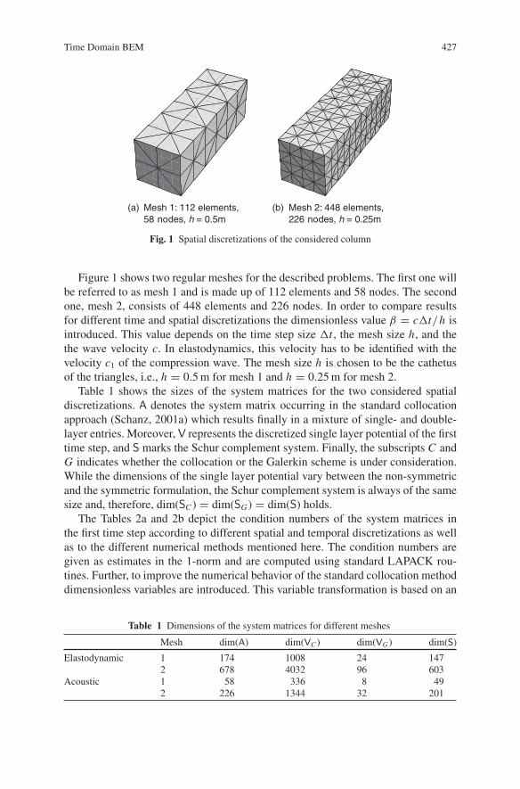
(a) Mesh 1: 112 elements,58 nodes, h = 0.5m

(b) Mesh 2: 448 elements,226 nodes, h = 0.25m

Fig. 1 Spatial discretizations of the considered column

Figure 1 shows two regular meshes for the described problems. The first one willbe referred to as mesh 1 and is made up of 112 elements and 58 nodes. The secondone, mesh 2, consists of 448 elements and 226 nodes. In order to compare resultsfor different time and spatial discretizations the dimensionless value β = cΔt/h isintroduced. This value depends on the time step size Δt , the mesh size h, and thethe wave velocity c. In elastodynamics, this velocity has to be identified with thevelocity c1 of the compression wave. The mesh size h is chosen to be the cathetusof the triangles, i.e., h = 0.5 m for mesh 1 and h = 0.25 m for mesh 2.

Table 1 shows the sizes of the system matrices for the two considered spatialdiscretizations. A denotes the system matrix occurring in the standard collocationapproach (Schanz, 2001a) which results finally in a mixture of single- and double-layer entries. Moreover, V represents the discretized single layer potential of the firsttime step, and S marks the Schur complement system. Finally, the subscripts C andG indicates whether the collocation or the Galerkin scheme is under consideration.While the dimensions of the single layer potential vary between the non-symmetricand the symmetric formulation, the Schur complement system is always of the samesize and, therefore, dim(SC ) = dim(SG) = dim(S) holds.

The Tables 2a and 2b depict the condition numbers of the system matrices inthe first time step according to different spatial and temporal discretizations as wellas to the different numerical methods mentioned here. The condition numbers aregiven as estimates in the 1-norm and are computed using standard LAPACK rou-tines. Further, to improve the numerical behavior of the standard collocation methoddimensionless variables are introduced. This variable transformation is based on an

Table 1 Dimensions of the system matrices for different meshes

Mesh dim(A) dim(VC ) dim(VG ) dim(S)

Elastodynamic 1 174 1008 24 1472 678 4032 96 603

Acoustic 1 58 336 8 492 226 1344 32 201

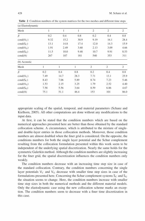
428 M. Schanz et al.

Table 2 Condition numbers of the system matrices for the two meshes and different time steps

(a) Elastodynamic

Mesh 1 1 1 2 2 2

β 0.2 0.4 0.8 0.2 0.4 0.8

cond(VC) 9.32 15.2 30.9 9.19 16.1 28.4

cond(SC) 13.1 14.8 17.4 12.0 14.3 15.9

cond(VG) 1.91 2.49 3.60 2.13 3.09 4.66

cond(SG) 11.5 10.0 9.48 10.7 9.91 8.53

cond(A) 267 187 181 540 353 311

(b) Acoustic

Mesh 1 1 1 2 2 2

β 0.2 0.4 0.8 0.2 0.4 0.8

cond(VC) 7.49 14.7 28.3 7.71 13.1 25.9

cond(SC) 8.43 7.06 5.89 8.74 7.23 5.46

cond(VG) 1.53 2.15 3.25 1.79 2.52 4.40

cond(SG) 7.58 5.56 3.64 8.59 6.86 4.67

cond(A) 75.1 51.1 46.4 153 101 86.0

appropriate scaling of the spatial, temporal, and material parameters (Schanz andKielhorn, 2005). All other computations are done without any modifications to theinput data.

At first, it can be stated that the condition numbers which are based on thenumerical approaches presented here are better than those obtained by the standardcollocation scheme. A circumstance, which is attributed to the mixture of single-and double-layer entries in those collocation methods. Moreover, those conditionnumbers are almost doubled when the finer grid is considered. On the opposite, theconditions numbers for both the single layer potential and the Schur complementresulting from the collocation formulation presented within this work seem to beindependent of the underlying spatial discretization. Nearly the same holds for thesymmetric Galerkin method. Although the condition numbers are slightly increasingfor the finer grid, the spatial discretization influences the condition numbers onlyweakly.

The condition numbers decrease with an increasing time step size in case ofthe standard collocation. Contrary, the condition numbers concerning the singlelayer potentials VC and VG decrease with smaller time step sizes in case of theformulations presented here. Concerning the Schur complement systems SC and SG

the situation seems to change. Here, the condition numbers increase with smallertime step sizes in both the numerical methods and the different material models.Only the elastodynamic case using the new collocation scheme marks an excep-tion. The condition numbers seem to decrease with a finer time discretization inthis case.

Time Domain BEM 429

Next, only elastodynamic results are reported because the acoustic results arecomparable. Figure 2 depicts the displacement and traction solution with respect toall numerical methods mentioned here. Moreover, those solutions are based on mesh1 and vary in the temporal discretizations.

(a) Displacement solution at the free end

(b) Traction solution at the fixed end

Fig. 2 Elastodynamic solutions for different time step sizes (Mesh 1)

First of all, it can be stated that, in general, a finer time discretization yieldsbetter results for all considered numerical methods. Nevertheless, there are somedifferences between them. For instance, considering the displacement solution in

430 M. Schanz et al.

(a) Displacement solution at the free end

(b) Traction solution at the fixed end

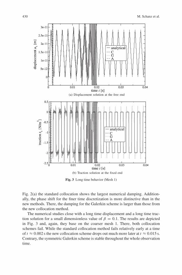
Fig. 3 Long time behavior (Mesh 1)

Fig. 2(a) the standard collocation shows the largest numerical damping. Addition-ally, the phase shift for the finer time discretization is more distinctive than in thenew methods. There, the damping for the Galerkin scheme is larger than those fromthe new collocation method.

The numerical studies close with a long time displacement and a long time trac-tion solution for a small dimensionless value of β = 0.1. The results are depictedin Fig. 3 and, again, they base on the coarser mesh 1. There, both collocationschemes fail. While the standard collocation method fails relatively early at a timeof t ≈ 0.002 s the new collocation scheme drops out much more later at t ≈ 0.015 s.Contrary, the symmetric Galerkin scheme is stable throughout the whole observationtime.

Time Domain BEM 431

5 Conclusions

To summarize the results, it can be concluded that due to the well structured sys-tem matrices the numerical methods presented here yield better stability propertiesthan the standard collocation scheme does. Nevertheless, those both methods havetheir drawbacks. For instance, the new collocation scheme results in quite largesystem matrices while the symmetric Galerkin scheme requires the evaluation ofthe hypersingular integral kernel and involves more costly double integrations. Butin the future, these additional computational costs should be reduced by, e.g., theapplication of some fast methods like adaptive cross approximation (Bebendorf andRjasanow, 2003). Fast methods are known to be much more efficient if well struc-tured systems are considered. Therefore, the new Collocation method as well as thesymmetric Galerkin scheme exhibit good optimization capabilities.

References

S. Ahmad and G.D. Manolis. Dynamic analysis of 3-D structures by a transformed boundaryelement method. Comput. Mech., 2:185–196, 1987.

H. Antes. A boundary element procedure for transient wave propagations in two-dimensionalisotropic elastic media. Finite Elem. Anal. Des., 1:313–322, 1985.

H. Antes and M. Jager. On stability and efficiency of 3d acoustic BE procedures for moving noisesources. In S.N. Atluri, G. Yagawa, and T.A. Cruse, editors, Computational Mechanics, Theoryand Applications, vol. 2, 3056–3061, Heidelberg, 1995. Springer-Verlag.

M. Bebendorf and S. Rjasanow. Adaptive low-rank approximation of collocation matrices.Computing, 70:1–24, 2003.

D.E. Beskos. Boundary element methods in dynamic analysis. AMR, 40(1):1–23, 1987.D.E. Beskos. Boundary element methods in dynamic analysis: Part II (1986–1996). AMR, 50(3):

149–197, 1997.M. Bonnet, G. Maier, and C. Polizzotto. Symmetric galerkin boundary element methods. AMR,

51(11):669–704, 1998.T.A. Cruse and F.J. Rizzo. A direct formulation and numerical solution of the general transient

elastodynamic problem, I. Aust. J. Math. Anal. Appl., 22(1):244–259, 1968.J. Domınguez. Dynamic stiffness of rectangular foundations. Report no. R78-20, Department of

Civil Engineering, MIT, Cambridge MA, 1978.J. Domınguez. Boundary Elements in Dynamics. Computational Mechanics Publication,

Southampton, 1993.A. Frangi and G. Novati. Regularized symmetric Galerkin BIE formulations in the Laplace

transform domain for 2D problems. Comput. Mech., 22:50–60, 1998.K.F. Graff. Wave Motion in Elastic Solids. Oxford University Press, 1975.E. Kausel. Fundamental Solutions in Elastodynamics. Cambridge University Press, 2006.L. Kielhorn and M. Schanz. Convolution Quadrature Method based symmetric Galerkin Boundary

Element Method for 3-d elastodynamics. Int. J. Numer. Methods. Engrg., 76(11):1724–1746,2008.

V.D. Kupradze, T.G. Gegelia, M.O. Basheleishvili, and T.V. Burchuladze. Three-DimensionalProblems of the Mathematical Theory of Elasticity and Thermoelasticity, vol 25 of AppliedMathematics and Mechanics. North-Holland, Amsterdam, New York, Oxford, 1979.

C. Lubich. Convolution quadrature and discretized operational calculus. I/II. Numer. Math., 52:129–145/413–425, 1988.

G.D. Manolis. A comparative study on three boundary element method approaches to problems inelastodynamics. Int. J. Numer. Methods. Engrg., 19:73–91, 1983.

432 M. Schanz et al.

W.J. Mansur. A Time-Stepping Technique to Solve Wave Propagation Problems Using theBoundary Element Method. Phd thesis, University of Southampton, 1983.

W.J. Mansur, J.A.M. Carrer, and E.F.N. Siqueira. Time discontinuous linear traction approximationin time-domain BEM scalar wave propagation. Int. J. Numer. Methods. Engrg., 42(4):667–683,1998.

G.V. Narayanan and D.E. Beskos. Numerical operational methods for time-dependent linearproblems. Int. J. Numer. Methods. Engrg., 18:1829–1854, 1982.

D. Nardini and C.A. Brebbia. A new approach to free vibration analysis using boundary elements.In C.A. Brebbia, editor, Boundary Element Methods, 312–326. Springer-Verlag, Berlin, 1982.

J.C. Nedelec. Integral equations with non integrable kernels. Integr. Equ. Oper. Theory, 5:563–672,1982.

P.W. Partridge, C.A. Brebbia, and L.C. Wrobel. The Dual Reciprocity Boundary Element Method.Computational Mechanics Publication, Southampton, 1992.

A. Peirce and E. Siebrits. Stability analysis and design of time-stepping schemes for generalelastodynamic boundary element models. Int. J. Numer. Methods. Engrg., 40(2):319–342,1997.

D.C. Rizos and D.L. Karabalis. An advanced direct time domain BEM formulation for general3-D elastodynamic problems. Comput. Mech., 15:249–269, 1994.

M. Schanz. Application of 3-d Boundary Element formulation to wave propagation in poroelasticsolids. Eng. Anal. Bound. Elem., 25(4–5):363–376, 2001a.

M. Schanz. Wave Propagation in Viscoelastic and Poroelastic Continua: A Boundary ElementApproach, vol 2 of Lecture Notes in Applied Mechanics. Springer-Verlag, Berlin, Heidelberg,New York, 2001b.

M. Schanz and H. Antes. Application of ‘operational quadrature methods’ in time domainboundary element methods. Meccanica, 32(3):179–186, 1997.

M. Schanz and L. Kielhorn. Dimensionless variables in a poroelastodynamic time domainboundary element formulation. Build. Res. J., 53(2–3):175–189, 2005.

O. Steinbach. Numerical Approximation Methods for Elliptic Boundary Value Problems, vol 54of Texts in Applied Mathematics. Springer, 2008.

L.T. Wheeler and E. Sternberg. Some theorems in classical elastodynamics. Arch. Rational Mech.Anal., 31:51–90, 1968.

G. Yu, W.J. Mansur, J.A.M. Carrer, and L. Gong. Time weighting in time domain BEM. Eng.Anal. Bound. Elem., 22(3):175–181, 1998.

G. Yu, W.J. Mansur, J.A.M. Carrer, and L. Gong. Stability of Galerkin and Collocation timedomain boundary element methods as applied to the scalar wave equation. Comput. Struct., 74(4):495–506, 2000.