Time Series Classification from Scratch with DeepNeural Networks: A Strong Baseline

Zhiguang Wang, Weizhong YanGE Global Research

{zhiguang.wang, yan}@ge.com

Tim OatesComputer Science and Electric EngineeringUniversity of Maryland Baltimore County

oates@umbc.edu

Abstract—We propose a simple but strong baseline for timeseries classification from scratch with deep neural networks. Ourproposed baseline models are pure end-to-end without any heavypreprocessing on the raw data or feature crafting. The proposedFully Convolutional Network (FCN) achieves premium perfor-mance to other state-of-the-art approaches and our explorationof the very deep neural networks with the ResNet structure isalso competitive. The global average pooling in our convolutionalmodel enables the exploitation of the Class Activation Map(CAM) to find out the contributing region in the raw data forthe specific labels. Our models provides a simple choice forthe real world application and a good starting point for thefuture research. An overall analysis is provided to discuss thegeneralization capability of our models, learned features, networkstructures and the classification semantics.

I. INTRODUCTION

Time series data is ubiquitous. Both human activities andnature produces time series everyday and everywhere, likeweather readings, financial recordings, physiological signalsand industrial observations. As the simplest type of time seriesdata, univariate time series provides a reasonably good start-ing point to study such temporal signals. The representationlearning and classification research has found many potentialapplication in the fields like finance, industry, and health care.

However, learning representations and classifying time se-ries are still attracting much attention. As the earliest baseline,distance-based methods work directly on raw time serieswith some pre-defined similarity measures such as Euclideandistance or Dynamic time warping (DTW) [1] to performclassification. The combination of DTW and the k-nearest-neighbors classifier is known to be a very efficient approachas a golden standard in the last decade.

Feature-based methods suppose to extract a set of featuresthat are able to represent the global/local time series patterns.Commonly, these features are quantized to form a Bag-of-Words (BoW), then given to the classifiers [2]. Feature-basedapproaches mostly differ in the extracted features. To namea few recent benchmarks, The bag-of-features framework(TSBF) [3] extracts the interval features with different scalesfrom each interval to form an instance, and each time seriesforms a bag. A supervised codebook is built with the randomforest for classifying the time series. Bag-of-SFA-Symbols(BOSS) [4] proposes a distance based on the histogramsof symbolic Fourier approximation words. Its extension, theBOSSVS method [5] combines the BOSS model with the

vector space model to reduce the time complexity and improvethe performance by ensembling the models with differencewindow size. The final classification is performed with theOne-Nearest-Neighbor classifier.

Ensemble based approaches combine different classifierstogether to achieve a higher accuracy. Different ensembleparadigms integrate various feature sets or classifiers. TheElastic Ensemble (PROP) [6] combines 11 classifiers based onelastic distance measures with a weighted ensemble scheme.Shapelet ensemble (SE) [7] produces the classifiers throughthe shapelet transform in conjunction with a heterogeneousensemble. The flat collective of transform-based ensembles(COTE) is an ensemble of 35 different classifiers based on thefeatures extracted from both the time and frequency domains.

All the above approaches need heavy crafting on datapreprocessing and feature engineering. Recently, some efforthas been spent to exploit the deep neural network, especiallyconvolutional neural networks (CNN) for end-to-end timeseries classification. In [8], a multi-channel CNN (MC-CNN)is proposed for multivariate time series classification. Thefilters are applied on each single channel and the features areflattened across channels as the input to a fully connectedlayer. The authors applied sliding windows to enhance thedata. They only evaluate this approach on two multivariatetime series datasets, where there is no published benchmarkfor comparison. In [9], the author proposed a multi-scale CNNapproach (MCNN) for univariate time series classification.Down sampling, skip sampling and sliding windows are usedfor preprocessing the data to manually prepare for the multi-scale settings. Although this approach claims the state-of-the-art performance on 44 UCR time series datasets [10], the heavypreprocessing efforts and a large set of hyperparameters makeit complicated to deploy. The proposed window slicing methodfor data augmentation seems to be ad-hoc.

We provide a standard baseline to exploit deep neuralnetworks for end-to-end time series classification without anycrafting in feature engineering and data preprocessing. Thedeep multilayer perceptrons (MLP), fully convolutional net-works (FCN) and the residual networks (ResNet) are evaluatedon the same 44 benchmark datasets with other benchmarks.Through a pure end-to-end training on the raw time seriesdata , the ResNet and FCN achieve comparable or betterperformance than COTE and MCNN. The global averagepooling in our convolutional model enables the exploitation of

arX

iv:1

611.

0645

5v4

[cs

.LG

] 1

4 D

ec 2

016

50

0

Inp

ut

50

0

50

0

Soft

max

Inp

ut

Soft

max

0.1 0.2 0.2 0.3

ReL

U

ReL

U

ReL

U

128

BN

+ R

eLU

256

BN

+ R

eLU

128

BN

+ R

eLU

Inp

ut

64

BN

+ R

eLU

64

BN

+ R

eLU

64

BN

+ R

eLU

Glo

bal

Po

olin

g

128B

N +

ReL

U128

BN

+ R

eLU

128

BN

+ R

eLU

128

BN

+ R

eLU

128

BN

+ R

eLU

128

BN

+ R

eLU

Soft

max

Glo

bal

Po

olin

g

+ + +

(a)MLP

(b)FCN

(C)ResNet

Fig. 1. The network structure of three tested neural networks. Dash line indicates the operation of dropout.

the Class Activation Map (CAM) to find out the contributingregion in the raw data for the specific labels.

II. NETWORK ARCHITECTURES

We tested three deep neural network architectures to providea fully comprehensive baseline.

A. Multilayer Perceptrons

Our plain baselines are basic MLP by stacking three fully-connected layers. The fully-connected layers each has 500neurons following two design rules: (i) using dropout [11]at each layer’s input to improve the generalization capability ;and (ii) the non-linearity is fulfilled by the rectified linear unit(ReLU)[12] as the activation function to prevent saturation ofthe gradient when the network is deep. The network ends witha softmax layer. A basic layer block is formalized as

x = fdropout,p(x)

y = W · x+ b

h = ReLU(y) (1)

This architecture is mostly distinguished from the seminalMLP decades ago by the utilization of ReLU and dropout.ReLU helps to stack the networks deeper and dropout largelyprevent the co-adaption of the neurons to help the modelgeneralizes well especially on some small datasets. However,if the network is too deep, most neuron will hibernate as theReLU totally halve the negative part. The Leaky ReLU [13]might help, but we only use three layers MLP with the ReLUto provide a fundamental baselines. The dropout rates at the

input layer, hidden layers and the softmax layer are {0.1, 0.2,0.3}, respectively (Figure 1(a)).

B. Fully Convolutional Networks

FCN has shown compelling quality and efficiency for se-mantic segmentation on images [14]. Each output pixel is aclassifier corresponding to the receptive field and the networkscan thus be trained pixel-to-pixel given the category-wisesemantic segmentation annotation.

In our problem settings, the FCN is performed as a featureextractor. Its final output still comes from the softmax layer.The basic block is a convolutional layer followed by a batchnormalization layer [15] and a ReLU activation layer. Theconvolution operation is fulfilled by three 1-D kernels with thesizes {8, 5, 3} without striding. The basic convolution blockis

y = W ⊗ x+ b

s = BN(y)

h = ReLU(s) (2)

⊗ is the convolution operator. We build the final networksby stacking three convolution blocks with the filter sizes {128,256, 128} in each block. Unlike the MCNN and MC-CNN, Weexclude any pooling operation. This strategy is also adopted inthe ResNet [16] as to prevent overfitting. Batch normalizationis applied to speed up the convergence speed and help improvegeneralization. After the convolution blocks, the features arefed into a global average pooling layer [17] instead of a fully

connected layer, which largely reduces the number of weights.The final label is produced by a softmax layer (Figure 1(b)).

C. Residual Network

ResNet extends the neural networks to a very deep structuresby adding the shortcut connection in each residual block toenable the gradient flow directly through the bottom layers.It achieves the state-of-the-art performance in object detectionand other vision related tasks [16]. We explore the ResNetstructure since we are really interested to see how the verydeep neural networks perform on the time series data. Ob-viously, the ResNet overfits the training data much easierbecause the datasets in UCR is comparatively small and lackof enough variants to learn the complex structures with suchdeep networks, but it is still a good practice to import themuch deeper model and analyze the pros and cons.

We reuse the convolutional blocks in Equation 2 to buildeach residual block. Let Blockk denotes the convolutionalblock with the number of filters k, the residual block isformalized as

h1 = Blockk1(x)

h2 = Blockk2(h1)

h3 = Blockk3(h2)

y = h3 + x

h = ReLU(y) (3)

The number of filters ki = {64, 128, 128}. The final ResNetstacks three residual blocks and followed by a global averagepooling layer and a softmax layer. As this setting simply reusesthe structures of the FCN, certainly there are better structuresfor the problem, but our given structures are adequate toprovide a qualified demonstration as a baseline (Figure 1(c)).

III. EXPERIMENTS AND RESULTS

A. Experiment Settings

We test our proposed neural networks on the same subsetof the UCR time series repository, which includes 44 distincttime series datasets, to compare with other benchmarks. Allthe dataset has been split into training and testing by default.The only preprocessing in our experiment is z-normalizationon both training and test split with the mean and standarddeviation of the training part for each dataset. The MLP istrained with Adadelta [18] with learning rate 0.1, ρ = 0.95and ε = 1e− 8. The FCN and ResNet are trained with Adam[19] with the learning rate 0.001, β1 = 0.9, β2 = 0.999 andε = 1e−8. The loss function for all tested model is categoricalcross entropy. We choose the best model that achieves thelowest training loss and report its performance on the testset. While this training setting tends to give us a overfittedconfiguration and most likely to generalize poorly on thetest set, we can see that our proposed networks generalizequite well. Unlike other benchmarks, our experiment excludesthe hyperparameter tuning and cross validation to providea most unbiased baseline. Such settings also largely reduce

the complexity for training and deploying the deep learningmodels. 1

B. Evaluation

Table I shows the results and a comprehensive comparisonwith eight other best benchmark methods. We report the testerror rate from the best model trained with the minimum cross-entropy loss and the number of dataset on which it achievedthe best performance. Some literature (like [9], [5]) also reportthe ranks and other ranking-based statistics to evaluate theperformance and make the comparison, so we also providethe average rankings.

However, neither the number of best-performed datasetor the ranking based statistics is an unbiased measurementto compare the performance. The number of best-performeddataset focuses on the top performance and is highly skewed.The ranking based statistics is highly sensitive to the modelpools. ”Better than” as a comparative measurement is alsoskewed as the input models might arbitrarily changed. Allthose evaluation measures wipe out the factor of number ofclasses.

We propose a simple evaluation measure, Mean Per-ClassError (MPCE) to evaluate the classification performance ofthe specific models on multiple datasets. For a given modelM = {mi}, a dataset pool D = {dk} with the number of classlabel C = {ck} and the corresponding error rate E = {ek},

PCEk =ekck

MPCEi =1

K

∑PCEk (4)

k refers to each dataset and i denotes to each model. Theintuition behind MPCE is simple: the expected error rate for asingle class across all the datasets. By considering the numberof classes, MPCE is more robust as a baseline criterion. Apaired T-test on PCE identifies if the differences of the MPCEare significant across different models.

C. Results and Analysis

We select seven existing best methods2 that claim the state-of-the-art results and published within recent three years: timeseries based on a bag-offeatures (TSBF), Elastic Ensemble(PROP), 1-NN Bag-Of-SFA-Symbols (BOSS) in Vector Space(BOSSVS), the Shapelet Ensemble (SE1) model, flat-COTE(COTE) and multi-scale CNN (MCNN). Note that COTE isan ensemble model which combines the weighted votes over35 different classifiers. BOSSVS is an ensemble of multipleBOSS models with different window length. 1NN-DTW isalso included as a simple standard baseline. The training anddeploying complexity of our models are small like 1NN-DTW

1The codes are available at https://github.com/cauchyturing/UCR Time Series Classification Deep Learning Baseline [20].

2’Best’ means the overall performance is competitive and the model shouldachieve the best performance on at least 4 datasets (10% of the all the 44datasets).

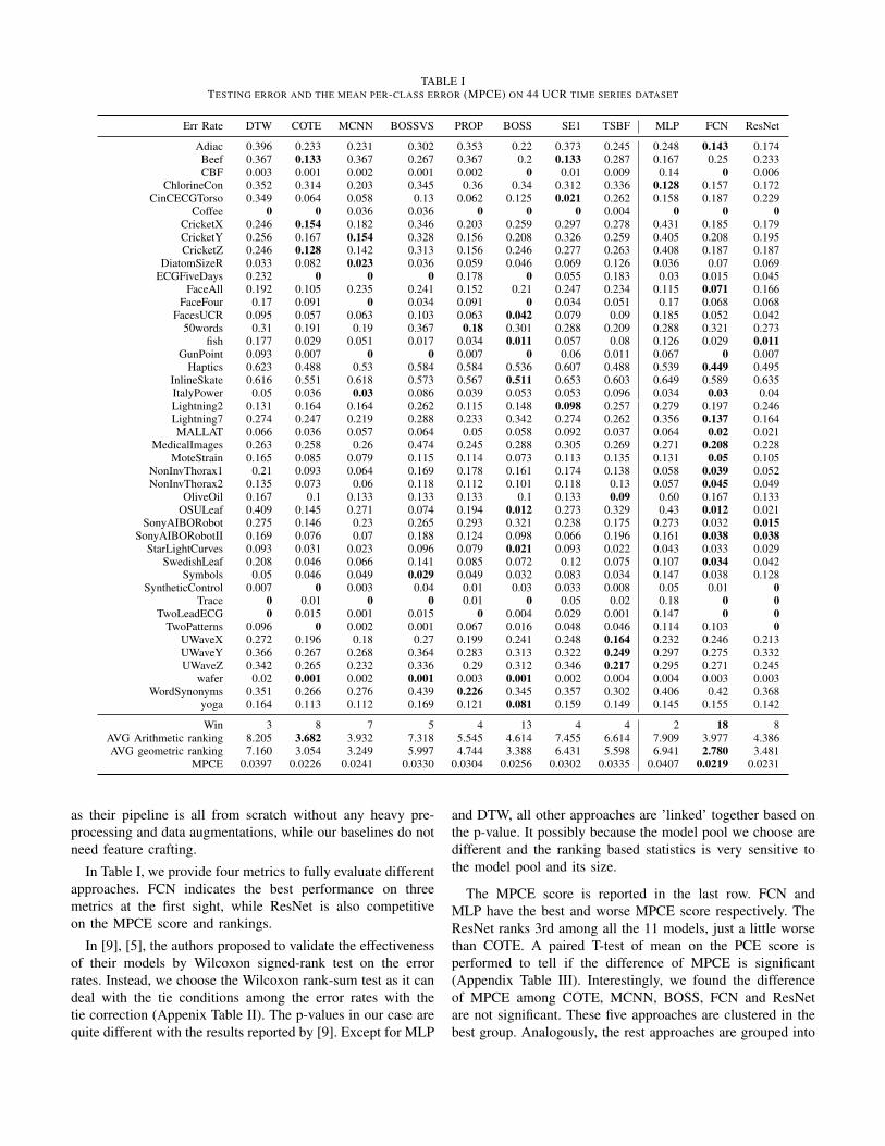
TABLE ITESTING ERROR AND THE MEAN PER-CLASS ERROR (MPCE) ON 44 UCR TIME SERIES DATASET

Err Rate DTW COTE MCNN BOSSVS PROP BOSS SE1 TSBF MLP FCN ResNet

Adiac 0.396 0.233 0.231 0.302 0.353 0.22 0.373 0.245 0.248 0.143 0.174Beef 0.367 0.133 0.367 0.267 0.367 0.2 0.133 0.287 0.167 0.25 0.233CBF 0.003 0.001 0.002 0.001 0.002 0 0.01 0.009 0.14 0 0.006

ChlorineCon 0.352 0.314 0.203 0.345 0.36 0.34 0.312 0.336 0.128 0.157 0.172CinCECGTorso 0.349 0.064 0.058 0.13 0.062 0.125 0.021 0.262 0.158 0.187 0.229

Coffee 0 0 0.036 0.036 0 0 0 0.004 0 0 0CricketX 0.246 0.154 0.182 0.346 0.203 0.259 0.297 0.278 0.431 0.185 0.179CricketY 0.256 0.167 0.154 0.328 0.156 0.208 0.326 0.259 0.405 0.208 0.195CricketZ 0.246 0.128 0.142 0.313 0.156 0.246 0.277 0.263 0.408 0.187 0.187

DiatomSizeR 0.033 0.082 0.023 0.036 0.059 0.046 0.069 0.126 0.036 0.07 0.069ECGFiveDays 0.232 0 0 0 0.178 0 0.055 0.183 0.03 0.015 0.045

FaceAll 0.192 0.105 0.235 0.241 0.152 0.21 0.247 0.234 0.115 0.071 0.166FaceFour 0.17 0.091 0 0.034 0.091 0 0.034 0.051 0.17 0.068 0.068

FacesUCR 0.095 0.057 0.063 0.103 0.063 0.042 0.079 0.09 0.185 0.052 0.04250words 0.31 0.191 0.19 0.367 0.18 0.301 0.288 0.209 0.288 0.321 0.273

fish 0.177 0.029 0.051 0.017 0.034 0.011 0.057 0.08 0.126 0.029 0.011GunPoint 0.093 0.007 0 0 0.007 0 0.06 0.011 0.067 0 0.007

Haptics 0.623 0.488 0.53 0.584 0.584 0.536 0.607 0.488 0.539 0.449 0.495InlineSkate 0.616 0.551 0.618 0.573 0.567 0.511 0.653 0.603 0.649 0.589 0.635ItalyPower 0.05 0.036 0.03 0.086 0.039 0.053 0.053 0.096 0.034 0.03 0.04Lightning2 0.131 0.164 0.164 0.262 0.115 0.148 0.098 0.257 0.279 0.197 0.246Lightning7 0.274 0.247 0.219 0.288 0.233 0.342 0.274 0.262 0.356 0.137 0.164MALLAT 0.066 0.036 0.057 0.064 0.05 0.058 0.092 0.037 0.064 0.02 0.021

MedicalImages 0.263 0.258 0.26 0.474 0.245 0.288 0.305 0.269 0.271 0.208 0.228MoteStrain 0.165 0.085 0.079 0.115 0.114 0.073 0.113 0.135 0.131 0.05 0.105

NonInvThorax1 0.21 0.093 0.064 0.169 0.178 0.161 0.174 0.138 0.058 0.039 0.052NonInvThorax2 0.135 0.073 0.06 0.118 0.112 0.101 0.118 0.13 0.057 0.045 0.049

OliveOil 0.167 0.1 0.133 0.133 0.133 0.1 0.133 0.09 0.60 0.167 0.133OSULeaf 0.409 0.145 0.271 0.074 0.194 0.012 0.273 0.329 0.43 0.012 0.021

SonyAIBORobot 0.275 0.146 0.23 0.265 0.293 0.321 0.238 0.175 0.273 0.032 0.015SonyAIBORobotII 0.169 0.076 0.07 0.188 0.124 0.098 0.066 0.196 0.161 0.038 0.038

StarLightCurves 0.093 0.031 0.023 0.096 0.079 0.021 0.093 0.022 0.043 0.033 0.029SwedishLeaf 0.208 0.046 0.066 0.141 0.085 0.072 0.12 0.075 0.107 0.034 0.042

Symbols 0.05 0.046 0.049 0.029 0.049 0.032 0.083 0.034 0.147 0.038 0.128SyntheticControl 0.007 0 0.003 0.04 0.01 0.03 0.033 0.008 0.05 0.01 0

Trace 0 0.01 0 0 0.01 0 0.05 0.02 0.18 0 0TwoLeadECG 0 0.015 0.001 0.015 0 0.004 0.029 0.001 0.147 0 0

TwoPatterns 0.096 0 0.002 0.001 0.067 0.016 0.048 0.046 0.114 0.103 0UWaveX 0.272 0.196 0.18 0.27 0.199 0.241 0.248 0.164 0.232 0.246 0.213UWaveY 0.366 0.267 0.268 0.364 0.283 0.313 0.322 0.249 0.297 0.275 0.332UWaveZ 0.342 0.265 0.232 0.336 0.29 0.312 0.346 0.217 0.295 0.271 0.245

wafer 0.02 0.001 0.002 0.001 0.003 0.001 0.002 0.004 0.004 0.003 0.003WordSynonyms 0.351 0.266 0.276 0.439 0.226 0.345 0.357 0.302 0.406 0.42 0.368

yoga 0.164 0.113 0.112 0.169 0.121 0.081 0.159 0.149 0.145 0.155 0.142

Win 3 8 7 5 4 13 4 4 2 18 8AVG Arithmetic ranking 8.205 3.682 3.932 7.318 5.545 4.614 7.455 6.614 7.909 3.977 4.386AVG geometric ranking 7.160 3.054 3.249 5.997 4.744 3.388 6.431 5.598 6.941 2.780 3.481

MPCE 0.0397 0.0226 0.0241 0.0330 0.0304 0.0256 0.0302 0.0335 0.0407 0.0219 0.0231

as their pipeline is all from scratch without any heavy pre-processing and data augmentations, while our baselines do notneed feature crafting.

In Table I, we provide four metrics to fully evaluate differentapproaches. FCN indicates the best performance on threemetrics at the first sight, while ResNet is also competitiveon the MPCE score and rankings.

In [9], [5], the authors proposed to validate the effectivenessof their models by Wilcoxon signed-rank test on the errorrates. Instead, we choose the Wilcoxon rank-sum test as it candeal with the tie conditions among the error rates with thetie correction (Appenix Table II). The p-values in our case arequite different with the results reported by [9]. Except for MLP

and DTW, all other approaches are ’linked’ together based onthe p-value. It possibly because the model pool we choose aredifferent and the ranking based statistics is very sensitive tothe model pool and its size.

The MPCE score is reported in the last row. FCN andMLP have the best and worse MPCE score respectively. TheResNet ranks 3rd among all the 11 models, just a little worsethan COTE. A paired T-test of mean on the PCE score isperformed to tell if the difference of MPCE is significant(Appendix Table III). Interestingly, we found the differenceof MPCE among COTE, MCNN, BOSS, FCN and ResNetare not significant. These five approaches are clustered in thebest group. Analogously, the rest approaches are grouped into

Fig. 2. Models grouping by the paired T-test of means on the normalized PCE scores.

two clusters based on the T-test results of the MPCE scores(Figure 2).

In the best group, BOSS and COTE are all ensemble basedmodels. MCNN exploit convolutional networks but requiresheavy preprocessing in data transformation, downsampling andwindow slicing. Our proposed FCN and ResNet are able toclassify time series from scratch and achieves the premiumperformance. Compared to FCN, ResNet tends to overfit thedata much easier, but is still clustered in the first group withoutsignificant difference to other four best models. We also notethat the proposed three-layer MLP achieves comparable resultsto 1NN-DTW without significant difference. Recent advanceson ReLU and dropout work quite well in our experiments tohelp the MLP gain the similar performance with the previousbaseline.

IV. LOCALIZE THE CONTRIBUTING REGIONS WITH CLASSACTIVATION MAP

Another benefit of FCN with the global average poolinglayer is its natural extension, the class activation map (CAM)to interpret the class-specific region in the data [23].

For a given time series, let Sk(x) represent the activation offilter k in the last convolutional layer at temporal location x.For filter k, the output of the following global average poolinglayer is fk =

∑x Sk(x). Let wc

k indicate the weight of thefinal softmax function for the output from filter k and the classc, then the input of the final softmax function is

gc =∑k

wck

∑x

Sk(x)

=∑k

∑x

wckSk(x)

We can define Mc as the class activation map for class c,where each temporal element is given by

Mc =∑k

wckSk(x)

Hence Mc(x, y) directly indicates the importance of theactivation at temporal location xi leading to the classificationof a sequence of time series to class c. If the output of the lastconvolutional layer is not the same as the input, we can stillidentify the contributing regions most relevant to the particularcategory by simply upsampling the class activation map to thelength of the input time series.

In Figure 3, we show two examples of the CAMs outputusing the above approach. We can see that the discriminativeregions of the time series for the right classes are highlighted.We also highlight the differences in the CAMs for the differentlabels. The contributing regions for different categories aredifferent.

On the ’CBF’ dataset, label 0 is determined mostly by theregion where the sharp drop occurs. Sequences with label1 have the signature pattern of a sharp rise followed by asmoothly down trending. For label 2, the neural network isaddress more attention on the long plateau occurs around themiddle. The similar analysis is also applied to the contributingregion on the ’StarLightCurve’ dataset. However, the label 0and label 1 are quite similar in shapes, so the contributingmap of label 1 focus less on the smooth trends of drop downwhile label 0 attract the uniform attention as the signal is muchsmoother.

The CAM provides a natural way to find out the contributingregion in the raw data for the specific labels. This enablesclassification-trained convolutional networks to learn to local-ize without any extra effort. Class activation maps also allowus to visualize the predicted class scores on any given timeseries, highlighting the discriminative subsequences detectedby the convolutional networks. CAM also provide a way tofind a possible explanation on how the convolutional networkswork for the setting of classification.

V. DISCUSSION

A. Overfitting and Generalization

Neural networks is a strong universal approximator whichis known to overfit easily due to the large number of param-eters. In our experiments, the overfitting was expected to besignificant since the UCR time series data is small and wehave no validation/test settings, only choose the model withthe lowest training loss for test.

However, our models generalize quite well given that thetraining accuracy are almost all 100%. Dropout improvesthe generalization capability of MLP by a large margin.For the family of convolutional networks, batch normaliza-tion is known to help improve both the training speed andgeneralization. Another important reason is we replace thefully-connected layer by the global average pooling layerbefore the softmax layer, which greatly reduces the amount ofparameters. Thus, starting with the basic network structureswithout any data transformation and ensemble, our three

Label 0: 0.984 Label 1: 0.999 Label 2: 0.985

Label 0: 0.822 Label 1: 0.987 Label 2: 0.999

high

Low

Fig. 3. The class activation mapping (CAM) technique allows the classification-trained FCN to both classify the time series and localize class-specificregions in a single forward-pass. The plots give examples of the contributing regions of the ground truth label in the raw data on the ’CBF’ (above) and’StarLightCurve’ (below) dataset. The number indicates the likelihood of the corresponding label.

models provide very simple but strong baseline for time seriesclassification with the state-of-the-art performance.

Another nuance of our results is that, deep neural networkswork potentially quite well on small dataset as we expand theirgeneralization by recent advances in the network structures andother technical tricks.

B. Feature Visualization and Analysis

We adopt the Gramian Angular Summation Field (GASF)[21] to visualize the filters/weights in the neural networks.Given a series X = {x1, x2, ..., xn}, we rescale X so that allvalues fall in the interval [0, 1]

xi0 =xi −min(X)

max(X)−min(X)(5)

Then we can easily exploit the angular perspective byconsidering the trigonometric summation between each pointto identify the correlation within different time intervals. TheGASF are defined as

G =[cos(φi + φj)

](6)

= X ′ · X −√I − X2

′·√I − X2 (7)

I is the unit row vector [1, 1, ..., 1]. By defining the innerproduct < x, y >= x · y−

√1− x2 ·

√1− y2 and < x, y >=√

1− x2 · y − x ·√1− y2,GASF are actually quasi-Gramian

matrices [< x1, x1 >].

We choose GASF because it provides an intuitive way to in-terpret the multi-scale correlation in 1-D space. G(i,j||i−j|=k)

encodes the cosine summation over the points with the stridingstep k . The main diagonal Gi,i is the special case when k = 0which contains the original values.

Figure 4 provides a visual demonstration of the filters inthree tested models. The weights from the second and thelast layer in MLP are very similar with clear structures andvery little degradation occurring. The weights in the first layer,generally, have the higher values than the following layers.

The filters in FCN and ResNet are very similar. Theconvolution extracts the local features in the temporal axis,essentially like a weighted moving average that enhancesseveral receptive fields with the nonlinear transformations bythe ReLU. The sliding filters consider the dependencies amongdifferent time intervals and frequencies. The filters learnedin the deeper layers are similar with their preceding layers.This suggests the local patterns across multiple convolutionallayers are seemingly homogeneous. Both the visualization andclassification performance indicates the effectiveness of the 1-D convolution.

C. Deep and Shallow

The exploration on the very deep architecture is interestingand informative. The ResNet model has 11 layers but stillholds the premium performance. There are two factors thatimpact the performance of the ResNet. With shortcut con-nections, the gradients can flow directly through the bottom

(a)MLP

(b)FCN

(C)ResNet

Fig. 4. Visualization of the filters learned in MLP, FCN and ResNet on the Adiac dataset. For ResNet, the three visualized filters are from the first, secondand third convolution layers in each residual blocks.

layers in the ResNet, which largely improve the interpretabilityof the model to learn some highly complex patterns in thedata. Meanwhile, the much deeper models tend to overfitmuch easier, requiring more effort in regularizing the modelto improve its generalization ability.

In our experiments, the batch normalization and globalaverage pooling have largely improved the performance intest data but still tend to overfit, as the patterns in the UCRdataset are comparably not so complex to catch. As a result,the test performance of the ResNet is not as good as FCN.When the data is larger and more complex, we encourage theexploration of the ResNet structure since it is more likely tofind a good trade-off between the strong interpretability andgeneralization.

D. Classification SemanticsThe benchmark approaches for time series classification

could be categorized into three groups: distance based, featurebased and neural neural network based. The combination ofdistance and feature based approaches are also commonlyexplored to improve the performance. We are curious aboutthe classification behavior of different models as if they all

perform similarly on the same dataset, or their feature spaceand learned classifier are diverged.

The semantics of different models are evaluated based ontheir PCE scores. We choose PCA to reduce the dimensionbecause this simple linear transformation is able to preserveslarge pairwise distances. In Figure 5, the distance betweenthree baseline models with other benchmarks are compar-atively large. which indicates the feature and classificationcriterion learned in our models are good complement to othermodels.

It is natural to see that FCN and ResNet are quite close witheach other. The embedding of MLP is isolated into a singlecategory, meaning its classification behavior is quite differentwith other approaches. This inspires us that a synthesis of thefeature learned by MLP and convolutional networks througha deep-and-wide model [22] might also improve the perfor-mance.

VI. CONCLUSIONS

We provide a simple and strong baseline for time seriesclassification from scratch with deep neural networks. Ourproposed baseline models are pure end-to-end without any

Fig. 5. The PCE distribution of different approaches after dimension reduction through PCA.

heavy preprocessing on the raw data or feature crafting. TheFCN achieves premium performance to other state-of-the-art approaches. Our exploration on the much deeper neuralnetworks with the ResNet structure also gets competitiveperformance under the same experiment settings. The globalaverage pooling in our convolutional model enables the ex-ploitation of the Class Activation Map (CAM) to find out thecontributing region in the raw data for the specific labels. Asimple MLP is found to be identical to the 1NN-DTW asthe previous golden baseline. An overall analysis is providedto discuss the generalization of our models, learned features,network structures and the classification semantics. Ratherthan ranking based criterion, MPCE is proposed as an unbiasedmeasurement to evaluate the performance of multiple modelson multiple datasets. Many research focus on time seriesclassification and recent effort is more and more lying on thedeep learning approach for the related tasks. Our baseline, withsimple protocol and small complexity for building and deploy-ing, provides a default choice for the real world applicationand a good starting point for the future research.

REFERENCES

[1] E. Keogh and C. A. Ratanamahatana, “Exact indexing of dynamic timewarping,” Knowledge and information systems, vol. 7, no. 3, pp. 358–386, 2005.

[2] J. Lin, E. Keogh, L. Wei, and S. Lonardi, “Experiencing sax: a novelsymbolic representation of time series,” Data Mining and knowledgediscovery, vol. 15, no. 2, pp. 107–144, 2007.

TABLE IIAPPENDIX: THE P-VALUES OF WILCOXON RANK-SUM TEST BETWEEN

OUR BASELINE MODELS WITH OTHER APPROACHES.

MLP FCN ResNet

DTW 0.7575 0.0203 0.0245COTE 0.0040 0.8445 0.8347

MCNN 0.0049 0.9834 0.9468BOSSVS 0.1385 0.1660 0.1887

PROP 0.0616 0.2529 0.2360BOSS 0.0076 0.8905 0.8740

SE1 0.1299 0.0604 0.0576TSBF 0.1634 0.0715 0.0811MLP / 0.0051 0.0049FCN 0.0051 / 0.9169

ResNet 0.0049 0.9169 /

[3] M. G. Baydogan, G. Runger, and E. Tuv, “A bag-of-features frameworkto classify time series,” IEEE transactions on pattern analysis andmachine intelligence, vol. 35, no. 11, pp. 2796–2802, 2013.

[4] P. Schafer, “The boss is concerned with time series classification in thepresence of noise,” Data Mining and Knowledge Discovery, vol. 29,no. 6, pp. 1505–1530, 2015.

[5] P. Schafer, “Scalable time series classification,” Data Mining andKnowledge Discovery, pp. 1–26, 2015.

[6] J. Lines and A. Bagnall, “Time series classification with ensemblesof elastic distance measures,” Data Mining and Knowledge Discovery,vol. 29, no. 3, pp. 565–592, 2015.

[7] A. Bagnall, J. Lines, J. Hills, and A. Bostrom, “Time-series classificationwith cote: the collective of transformation-based ensembles,” IEEETransactions on Knowledge and Data Engineering, vol. 27, no. 9, pp.2522–2535, 2015.

[8] Y. Zheng, Q. Liu, E. Chen, Y. Ge, and J. L. Zhao, “Exploiting multi-channels deep convolutional neural networks for multivariate time series

TABLE IIIAPPENDIX: THE P-VALUES OF THE PAIRED T-TEST OF THE MEANS FOR THE MPCE SCORE ON 11 BENCHMARK MODELS.

DTW COTE MCNN BOSSVS PROP BOSS SE1 TSBF MLP FCN ResNet

DTW 2.056E-05 5.699E-05 5.141E-02 4.832E-05 2.760E-04 3.040E-03 1.311E-02 4.234E-01 1.451E-04 3.427E-04COTE 2.287E-01 3.721E-05 5.911E-03 1.033E-01 1.208E-04 3.528E-04 5.240E-05 3.978E-01 4.351E-01

MCNN 3.652E-04 1.354E-02 2.497E-01 3.634E-03 3.360E-03 8.023E-05 2.495E-01 3.757E-01BOSSVS 2.140E-01 6.404E-04 1.763E-01 4.335E-01 4.628E-02 2.983E-03 5.067E-03

PROP 3.739E-02 4.654E-01 1.440E-01 2.061E-02 2.673E-02 4.241E-02BOSS 2.871E-02 1.759E-02 1.049E-03 1.879E-01 2.751E-01

SE1 1.770E-01 9.901E-03 1.208E-02 3.251E-02TSBF 7.088E-02 1.510E-03 1.640E-03MLP 6.832E-05 3.045E-04FCN 2.508E-01

ResNet

classification,” Frontiers of Computer Science, vol. 10, no. 1, pp. 96–112, 2016.

[9] Z. Cui, W. Chen, and Y. Chen, “Multi-scale convolutional neural net-works for time series classification,” arXiv preprint arXiv:1603.06995,2016.

[10] Y. Chen, E. Keogh, B. Hu, N. Begum, A. Bagnall, A. Mueen, andG. Batista, “The ucr time series classification archive (2015),” 2016.

[11] N. Srivastava, G. E. Hinton, A. Krizhevsky, I. Sutskever, andR. Salakhutdinov, “Dropout: a simple way to prevent neural networksfrom overfitting.” Journal of Machine Learning Research, vol. 15, no. 1,pp. 1929–1958, 2014.

[12] V. Nair and G. E. Hinton, “Rectified linear units improve restricted boltz-mann machines,” in Proceedings of the 27th International Conferenceon Machine Learning (ICML-10), 2010, pp. 807–814.

[13] B. Xu, N. Wang, T. Chen, and M. Li, “Empirical evaluation of rectifiedactivations in convolutional network,” arXiv preprint arXiv:1505.00853,2015.

[14] J. Long, E. Shelhamer, and T. Darrell, “Fully convolutional networksfor semantic segmentation,” in Proceedings of the IEEE Conference onComputer Vision and Pattern Recognition, 2015, pp. 3431–3440.

[15] S. Ioffe and C. Szegedy, “Batch normalization: Accelerating deepnetwork training by reducing internal covariate shift,” arXiv preprintarXiv:1502.03167, 2015.

[16] K. He, X. Zhang, S. Ren, and J. Sun, “Deep residual learning for imagerecognition,” arXiv preprint arXiv:1512.03385, 2015.

[17] M. Lin, Q. Chen, and S. Yan, “Network in network,” arXiv preprintarXiv:1312.4400, 2013.

[18] M. D. Zeiler, “Adadelta: an adaptive learning rate method,” arXivpreprint arXiv:1212.5701, 2012.

[19] D. Kingma and J. Ba, “Adam: A method for stochastic optimization,”arXiv preprint arXiv:1412.6980, 2014.

[20] F. Chollet, “Keras,” https://github.com/fchollet/keras, 2015.[21] Z. Wang and T. Oates, “Imaging time-series to improve classification

and imputation,” arXiv preprint arXiv:1506.00327, 2015.[22] H.-T. Cheng, L. Koc, J. Harmsen, T. Shaked, T. Chandra, H. Aradhye,

G. Anderson, G. Corrado, W. Chai, M. Ispir et al., “Wide & deeplearning for recommender systems,” in Proceedings of the 1st Workshopon Deep Learning for Recommender Systems. ACM, 2016, pp. 7–10.

[23] B. Zhou, A. Khosla, A. Lapedriza, A. Oliva, and A. Torralba,“Learning deep features for discriminative localization,” arXiv preprintarXiv:1512.04150, 2015.