NBER WORKING PAPER SERIES

TIME VARYING RISK AVERSION

Luigi GuisoPaola SapienzaLuigi Zingales

Working Paper 19284http://www.nber.org/papers/w19284

NATIONAL BUREAU OF ECONOMIC RESEARCH1050 Massachusetts Avenue

Cambridge, MA 02138August 2013

We thank Nick Barberis, John Campbell , James Dow, Stefan Nagel, and Ivo Welch for very helpfulcomments. We also benefited from comments from participants at seminars the University of ChicagoBooth, Boston College, University of Minnesota, University of Michigan, Hong Kong University,London Business School, Statistics Norway, The European Central Bank, University of Maastricht,the 2011 European Financial Association Meetings, the 201 2 European Economic Association Meetings,the April 2013 NBER Behavioral Finance Meeting, UCLA behavioral finance association, StanfordUniversity. Luigi Guiso gratefully acknowledges financial support from PEGGED, Paola Sapienzafrom the Zell Center for Risk and Research at Kellogg School of Management, and Luigi Zingalesfrom the Stigler Center and the Initiative on Global Markets at the University of Chicago Booth Schoolof Business. We thank Filippo Mezzanotti for excellent research assistantship, and Peggy Eppink foreditorial help. The views expressed herein are those of the authors and do not necessarily reflect theviews of the National Bureau of Economic Research.

NBER working papers are circulated for discussion and comment purposes. They have not been peer-reviewed or been subject to the review by the NBER Board of Directors that accompanies officialNBER publications.

© 2013 by Luigi Guiso, Paola Sapienza, and Luigi Zingales. All rights reserved. Short sections oftext, not to exceed two paragraphs, may be quoted without explicit permission provided that full credit,including © notice, is given to the source.

Time Varying Risk AversionLuigi Guiso, Paola Sapienza, and Luigi ZingalesNBER Working Paper No. 19284August 2013JEL No. D1,D8,G11,G12

ABSTRACT

We use a repeated survey of an Italian bank’s clients to test whether investors’ risk aversion increasesfollowing the 2008 financial crisis. We find that both a qualitative and a quantitative measure of riskaversion increases substantially after the crisis. After considering standard explanations, we investigatewhether this increase might be an emotional response (fear) triggered by a scary experience. To showthe plausibility of this conjecture, we conduct a lab experiment. We find that subjects who watcheda horror movie have a certainty equivalent that is 27% lower than the ones who did not, supportingthe fear-based explanation. Finally, we test the fear-based model with actual trading behavior andfind consistent evidence.

Luigi GuisoAxa Professor of Household FinanceEinaudi Institute for Economics and FinanceVia Sallustiana 62 - 00187Rome, Italyluigi.guiso@eief.it

Paola SapienzaKellogg School of ManagementNorthwestern University2001 Sheridan Road, Evanston, IL 60208and CEPRand also NBERpaola-sapienza@northwestern.edu

Luigi ZingalesBooth School of BusinessThe University of Chicago5807 S. Woodlawn AvenueChicago, IL 60637and NBERluigi.zingales@ChicagoBooth.edu

2

In a seminal paper, Fama (1984) shows that existing asset pricing models can explain the pattern of

exchange rate movements only by allowing for large changes in aggregate risk aversion. Since then,

many papers have shown that to fit the time series of aggregate U.S. stock prices, asset pricing

models require large fluctuations in the aggregate risk aversion.

To account for these fluctuations the literature has mainly focused on two (non-exclusive)

approaches. The first maintains the representative agent assumption, but introduces some variation

in the standard preferences to produce a higher curvature of the utility function (Campbell and

Cochrane, 1999; Barberis, Huang and Santos, 2001). The second abandons the representative agent

perspective and relies on agency problems in delegated asset management to explain the surge in

aggregate risk aversion during crises (Vayanos, 2004; He and Krishnamurthy, 2012). While the

mechanism underlying this latter literature is supported by some empirical evidence (Muir, 2013),

the basic assumption underpinning the first - that individual risk aversion surges during economic

crises - has not found much empirical support so far.

To address this gap, we analyze whether individual risk aversion increases following the

major economic crisis of the last 80 years - the 2008 financial crisis. We do so by exploiting some

survey-based measures of risk aversion elicited in a sample of clients of a large Italian bank in 2007

and repeated on the same set of people in 2009.

We find that both qualitative and quantitative measures of risk aversion exhibit large

increases following the crisis. The certainty equivalent of a risky gamble with an expected value of

5,000 euros drops from 4,000 euros to 2,500 euros, with 55% of the respondents exhibiting an

increase in this quantitative measure of risk aversion. Similarly, 46% of the respondents experience

an increase in a qualitative measure of risk aversion, which measures the individual’s willingness to

trade-off risk and return.

Having shown that individual risk aversion moves over time in a way consistent with a

change in the curvature of the utility function, we then try to see whether the existing models are

also able to explain the cross sectional variations. Neither changes in wealth (as a standard model

will predict) nor changes in total habit (as habit persistence would imply) seem to have any effect

on changes in risk aversion, regardless of the measure used. To test whether these changes are due

to variations in background risk, we look at retirees (who in Italy enjoy a public pension) and public

employees (who at the time faced little or no risk of layoffs) and find very similar results.

Subjective estimates of the expected return in the market and its expected volatility do not have any

explanatory power either.

Individuals who experience extraordinarily big losses seem to exhibit a greater increase in

the quantitative measure of risk aversion. This finding supports Barberis et al. (2001), who argue

3

that losses negatively affect investors' utility beyond the wealth implications of these losses. Yet,

our finding that risk aversion increases even among those who did not experience any loss suggests

that investors were emotionally affected by a stock market crash even if they were not financially

affected by it.

For this reason we explore whether an emotion-based framework can account for our results.

Our hypothesis draws on an influential paper by Loewenstein, et al. (2001) that distinguishes

between anticipated emotions and anticipatory emotions. Most of the economic models treat

emotions as part of the utility function: feelings are expected consequences of the outcomes and are

taken into account in decision making through a cognitive process. Alternatively, Loewenstein et al.

(2001) recognize that emotions are often experienced at the time of the decision and may lead to

action bypassing the cognitive process. In this framework, visceral factors (Loewenstein, 1996,

2000), such as fear, alter behavior rapidly with limited or no higher level cognitive deliberation

(LeDoux, 1996).

We consider the possibility that investors react to fear of large losses, even if they do not

experience them. To isolate this possible channel, we resort to a laboratory experiment based on a

fear conditioning model, where subjects are exposed to a horror movie that stimulates the emotion

of fear (Kinreich et al., 2012). The main advantage of an experiment is that it allows us to examine

the behavior of subjects while perfectly controlling for the outside environment. In so doing, it

allows us to mimic the situation of investors who are emotionally (but not financially) affected by a

stock market crash. The maintained assumption in this experiment is that the fear generated by the

horror movie in the lab acts in a similar way as the fear activated by watching the news about the

financial crisis.

We “treat” a sample of students with a five-minute excerpt from the movie, Hostel (2005,

directed by Eli Roth), characterized by stark and graphic images. It shows a young man inhumanly

tortured in a dark basement. We find that treated students exhibit a higher risk aversion (both

according to the quantitative and the qualitative measure) very similar to the one experienced by the

Italian bank’s clients in 2009. The treated subjects’ certainty equivalent is 27% lower than that of

untreated ones. Interestingly, the effect is entirely concentrated among students who dislike horror

movies. The ones who like them seem unaffected.

Since the outside environment of the treated and non-treated sample is the same, the

experiment is able to show that emotional fear (i.e. fear that is not related to changes in the outside

environment), experienced at the time of the decision, causes an increase in risk aversion. However,

we cannot directly measure whether the bank customer sample experienced fear during the financial

crisis. We can only establish whether their subsequent behavior is consistent with a fear based

4

model. While in a traditional Merton model investors facing a drop in equity prices should

rebalance their portfolio by buying more risky assets, a fear based model predicts that individuals

triggered by fear will rebalance their portfolio by selling risky assets. By using actual trades of the

bank’s clients we find evidence consistent with the latter hypothesis.

The paper closest to ours is Weber et al. (2011). In this paper, they survey online customers

of a brokerage account in England between September 2008 and June 2009. They find that while

risk taking decreases between September and March, their measures of risk attitudes do not. The

difference in the results can be due to three causes. First, their sample of online customers who

answer online surveys is likely to be biased in favor of risk takers who are less affected by negative

events. Second, their measures of risk attitudes are different and tend to mix expectations and risk

aversion. Third, the earlier measures are taken in September 2008 when the situation is already

problematic, while our measures are taken long before the inception of the crisis. Our paper is also

related to the literature on fear and risk aversion (e.g. Lerner and Keltner, 2000, 2001) and on the

effect of emotions on risk attitudes, portfolio choice, and stock returns (Kamstra et al., 2003 and

Kramer and Weber, 2012).

The rest of the paper continues as follows. Section 1 reviews how risk aversion can be

estimated. Section 2 describes the data. Section 3 presents the results about the changes in risk

aversion, while Section 4 tests for possible explanations of these changes. Section 5 discusses the

notion of fear and how fear can be induced in a lab experiment. Section 6 reports the results of this

experiment. Section 7 develops some testable implications of the trading behavior of investors

affected by fear and tests these implications on the Italian bank’s administrative data. Section 8

concludes.

1. Measuring individual risk aversion

If we want to test whether changes in risk aversion can explain movements in asset prices, we need

a way to infer risk aversion that is independent of asset prices. There exist two different approaches:

the first relies on a revealed preference strategy, the second on direct elicitation of risk attitudes

from choices in experiments or survey questions.

1.1 Revealed preferences

Friend and Blume (1975) were the first to infer an individual’s relative risk aversion from

his share of investments in risky assets. In Merton’s (1969) portfolio model, the share of wealth

invested in risky assets by individual i is

5

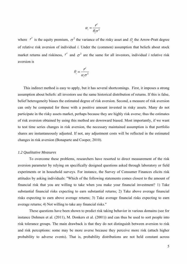
where er is the equity premium, the variance of the risky asset and the Arrow-Pratt degree

of relative risk aversion of individual i. Under the (common) assumption that beliefs about stock

market returns and riskiness, er and are the same for all investors, individual i relative risk

aversion is

This indirect method is easy to apply, but it has several shortcomings. First, it imposes a strong

assumption about beliefs: all investors use the same historical distribution of returns. If this is false,

belief heterogeneity biases the estimated degree of risk aversion. Second, a measure of risk aversion

can only be computed for those with a positive amount invested in risky assets. Many do not

participate in the risky assets market, perhaps because they are highly risk averse; thus the estimates

of risk aversion obtained by using this method are downward biased. Most importantly, if we want

to test time series changes in risk aversion, the necessary maintained assumption is that portfolio

shares are instantaneously adjusted. If not, any adjustment costs will be reflected in the estimated

changes in risk aversion (Bonaparte and Cooper, 2010).

1.2 Qualitative Measures

To overcome these problems, researchers have resorted to direct measurement of the risk

aversion parameter by relying on specifically designed questions asked through laboratory or field

experiments or in household surveys. For instance, the Survey of Consumer Finances elicits risk

attitudes by asking individuals: "Which of the following statements comes closest to the amount of

financial risk that you are willing to take when you make your financial investment? 1) Take

substantial financial risks expecting to earn substantial returns; 2) Take above average financial

risks expecting to earn above average returns; 3) Take average financial risks expecting to earn

average returns; 4) Not willing to take any financial risks."

These questions have been shown to predict risk taking behavior in various domains (see for

instance Dohmen et al. (2011), M. Donkers et al. (2001)) and can thus be used to sort people into

risk tolerance groups. The main drawback is that they do not distinguish between aversion to risk

and risk perceptions: some may be more averse because they perceive more risk (attach higher

probability to adverse events). That is, probability distributions are not held constant across

6

respondents. In addition they are hard to interpret as a preference parameter in the Arrow-Pratt

sense.

1.3 Quantitative measures

These problems can be dealt with by confronting individuals with specific risky prospects. Barsky

et al. (1997) use this approach to obtain a measure of relative risk aversion from respondents to the

Panel Study of Income Dynamics, by confronting them with the option of giving up their present

job with fixed salary for a (otherwise equivalent) job with uncertain lifetime earnings. Answers

allow them to bind the degree of relative risk aversion for the respondents into four intervals.

Guiso and Paiella (2008) recover a point estimate of an individual’s absolute risk aversion

by asking people in the SHIW (The Italian Survey of Households Income and Wealth) their

willingness to pay for a hypothetical lottery involving a gain of 5000 euros with probability ½.1

One advantage of these survey-based measures is that they are generally asked as part of a

long questionnaire, which can provide much individual-specific information. As a result, they can

be used to study the properties of the risk aversion function, in particular how it relates to an

individual's wealth, demographic characteristics, and the economic environment where he lives.

A third alternative that has been used to measure individual risk preferences and avoid

incentive effects is to rely on actual choices from such settings as people’s participation in

television games, (Beetsma and Schotman (2001), Bombardini and Trebbi (2011)), betting choices

in sports (Kopriva (2009), Andrikogiannopoulou (2010)), choices over menus of premiums and

deductibles in insurance contracts (Cohen and Einav (2007), Barseghyan et al. (2010)), and the

Lending Club (a peer-to-peer lending on the Web) investment choices (Parravicini and Ravina,

2010). Because actual money is involved, these studies are not subject to the incentive distortions of

hypothetical survey questions. This is not without cost, though. In some cases (as in television

games) relevant variables—such as people’s wealth and its composition—are not observed. Hence

measured risk preferences cannot be related to wealth. Second, these samples are not representative

of the population and can be highly selected (e.g. sport bettors), which makes it difficult to

extrapolate the findings to the general population. Third, in some of these instances measures of risk

preferences can only be obtained by restricting individuals beliefs, e.g. about the probability of an

accident (as in Cohen and Einav (2007), Barseghyan et al. (2010)) or the odds of a bet (as in

Andrikogiannopoulou (2010)).

1 Hartog and al. (2002) use a similar approach in a sample of Dutch accountants.

7

1.4 Our Choice

Our goal is to measure the risk aversion in a large sample of individual investors. Thus,

selection issues are very important and so are cost considerations. Individuals should be

approximately risk neutral over small gambles. Yet, offering large enough gambles to a large

sample is prohibitively expensive. For this reason, we resort to measuring risk aversion through a

survey. Surveys do suffer from the problem that they are pure hypothetical questions. To address

this problem we use questions that have been shown to result in reliable measures of risk aversions

and we validate them with actual data on portfolio choices.

2. Data Description

2.1 Sample

Our main data source is the second wave of the clients' survey run between June and September

2007 done by a large Italian bank. The survey is comprised of interviews with a sample of 1,686

Italian customers. The sample was stratified according to three criteria: geographical area, city size,

and financial wealth. To be included in the survey, customers must have had at least 10,000 euros

worth of assets with the bank at the end of 2006. The survey is described in greater detail in

Appendix 1 where we also compare it to the Bank of Italy survey.

Besides collecting detailed demographic information, data on investors’ financial

investments, information on beliefs, expectations, and risk perception, the survey collected data on

individual risk attitudes by asking both qualitative questions on people’s preferences regarding

risk/return combinations in financial decisions as well as their willingness to pay for a

(hypothetical) risky prospect. We describe these questions below.

For the sample of investors who participated in the 2007 survey, the bank gave us access to

the administrative records of the assets that these clients have with them. Specifically, we can

merge the survey data with administrative information on the stocks and on the net flows of 26

assets categories that investors have at the bank. We describe in detail this dataset and its content in

the Appendix. These data are available at monthly frequency for 35 months beginning in December

2006 and we use them to obtain measures of variation in wealth and portfolio investments over

time. Since some households left the bank after the interview, the administrative data are available

for 1,541 households instead of the 1,686 in the 2007 survey.

In order to study time variations in risk attitudes, in the spring of 2009 we asked the same

company that ran the 2007 survey to run a telephone survey on the sample of 1,686 investors

interviewed in 2007. The telephone survey was fielded in June 2009 and asked a much more

8

limited set of questions in a short 12-minute interview.2 Specifically, investors were asked two risk

aversion questions, a generalized trust question, a question about trust in their bank, and a question

about stock market expectations using exactly the same wording that was used to ask these

questions in the 2007 survey. Before asking the questions the interviewer made sure that the

respondent was the same person who answered the 2007 survey by collecting a number of

demographic characteristics and matching them with those from the 2007 survey.

Of the 1,686 who were contacted, roughly one third agreed to be re-interviewed so that we

end up with a two-year panel of 666 investors. Table I compares the characteristics of respondents

and non-respondents to the 2009 survey along several dimensions. In the first part of the table, we

compare the two samples according to the demographic characteristics collected in the 2007 survey

such as age, gender, marital status, geographical location, and education. The differences are small

and not statistically significant, with the exception of education where we cannot statistically reject

the hypothesis that the two samples differ. Still the economic magnitude of the difference is small

(less than a year of education).

In the middle part of the table, we compare the two samples according to their risk attitudes,

as measured in 2007. Along this dimension, which is the most important one for our analysis,

participants in the 2009 survey do not differ from non-participants. For instance, the average 2007

certainty equivalent for the hypothetical risky prospect (described below) is 3,278 euros among

non-respondents and 3,266 euros among respondents in the 2009 telephone survey.

While the two samples do not differ in observable characteristics in 2007, they might differ

in time-varying characteristics. For example, the crisis might have affected the two groups

differentially, in a way that is correlated with their willingness to be re-interviewed. Fortunately, we

have the administrative data (and hence the portfolio choices) of both the respondents and the non-

respondents both in 2007 and in 2009. Hence, the last part of Table I compares these choices. The

stock of financial assets, before and after the crisis, does not differ between the two groups, nor

does the fraction of wealth invested in stock. Similarly, there are no differences in the percentage

of people who own stock. From this we conclude that there does not seem to be any systematic

selection in the investors’ decisions to be re-interviewed in June 2009.

2.2. Measuring attitudes towards risk

The 2007 survey has two measures of risk attitudes. The first, patterned after a question in US

Survey of Consumer Finance, is a qualitative indicator of risk tolerance. Each participant is asked: 2 Since the second survey was filled during the same season as the first, the differences in risk aversion cannot be due to season variations in the length of day (see Kamstra et al. (2003)).

9

"Which of the following statements comes closest to the amount of financial risk that you are

willing to take when you make your financial investment: (1) a very high return, with a very high

risk of losing money; (2) high return and high risk; (3) moderate return and moderate risk; (4) low

return and no risk."

Only 18.6 percent of the sample chooses “low return and no risk,” so most are willing to

accept some risk if compensated by a higher return, but very few (1.8 percent) are ready to choose

very high risk and very high return. From this question we construct a categorical variable ranging

from 1 to 4 with larger values corresponding to greater dislike for risk.

In a world where people face the same risk-return tradeoffs and make portfolio decisions

according to Merton’s formula, their risk/return choice reflects their degree of relative risk aversion.

In such a world, the answers to the above questions can fully characterize people’s risk preferences.

However, if people differ in beliefs about stock market returns and/or volatility these differences

will contaminate their answers to the above question. This bias would affect not only cross-

sectional comparisons, but also inter-temporal ones, possibly revealing a change in risk preferences

when none is present.

The second measure of risk aversion contained in the 2007 survey helped us to deal with this

problem. Each respondent was presented with several choices between a risky prospect, which paid

10,000 euros or zero with equal probability and a sequence of certain sums of money. These sums

were progressively increasing between 100 euros and 9,000 euros. Since more risk averse people

will give up the risky prospect for lower certain sums, the first certain sum at which an investor

switches from the risky to the certain prospect identifies (an upper bound for) his/her certainty

equivalent. The question was framed so as to resemble a popular TV game (Affari Tuoi, the Italian

version of the TV game Deal or no Deal), analyzed by Bombardini and Trebbi (2010). Incidentally,

it is similar to the Holt and Laury (2002) strategy which has proved particularly successful in

overcoming the under/over-report bias implied when asking willingness to pay/accept.

Specifically, respondents were asked: “Imagine being in a room. To get out you have two

doors. Behind one of the two doors there is a 10,000 euro prize, behind the other nothing.

Alternatively, you can get out from the service door and win a known amount. If you were offered

100 euros, would you choose the service door? “

If he accepted 100 euros the interviewer moved on to the next question, otherwise he asked

whether the investor would accept 500 euros to exit the service door and if not 1500 and if not…,

3000, 4000, 5000, 5500, 7000, 9000, more than 9000 euros.

We code answers to this question both as the certainty equivalent value required by the

investor to give up the risky prospect as well as integers from 1 to 10 where 1 corresponds to a

10

certainty equivalent of 100 euros and 10 to a certainty equivalent larger than 9000 euros: the first is

decreasing in risk aversion, the second increasing.

We will refer to the measure based on preferences for risk-return combinations as the

qualitative indicator and to the one based on the lottery as the quantitative indicator. The first is a

measure of relative risk aversion measure, while the second is a measure of absolute risk aversion.

These two questions were asked both in the 2007 and the 2009 survey. Since the

hypothetical lottery faces each respondent with the same probabilities for the risky prospect,

differences in the certainty equivalent will reflect differences in risk preferences either across

individuals or over time for the same individual when we compare them across the 2007 and 2009

surveys.

The measure of risk aversion that is obtained should be thought of as a measure of the risk

aversion for the respondent’s value function and as such is potentially affected by any variable that

impacts people’s willingness to take risk, such as their wealth level or any background risk they

face. The summary statistics for these measures and all the other variables are contained in Table II.

2.3 Validating the risk aversion measures

A large and increasing literature shows that questions like the ones above predict risk taking

behavior in various domains (see for instance Dohmen et al. (2011), Donkers et al. (2001), Barsky

et al. (1997), Guiso and Paiella (2006, 2008)). They are also robust to the specific domain of risk:

using a panel of 20,000 German consumers Dohmen et al. (2011) show that indicators of risk

attitudes over different domains tend all to be correlated, with correlation coefficients of around 0.5

- a feature that is consistent with the idea that risk aversion is a personal trait.

To validate our measures, we run various tests. First, in Table III we document that our

qualitative and quantitative measures are positively correlated either when using the 2007 cross,

section (correlation coefficient 0.12) or the 2009 cross section (correlation 0.16) or when looking at

the correlation between the changes in the two measures between 2007 and 2009 (correlation

coefficient 0.12). Furthermore, in the 2009 survey we ask “After the stock market crash did you

become more cautious and prudent in your investment decisions?” The possible answers are: “More

or less like before,” “A bit more cautious,” or “Much more cautious.” Thirty-five percent of the

respondents declare to have become much more cautious, while 18% a bit more. If we create a

variable cautiousness equal to zero if the response is no change, 1 if the response is a bit more, and

2 if it is much more, we find that this variable has a 12% correlation (p-value 0.002) with the

changes in the qualitative measure of risk aversion and a 7.4% correlation (p-value 0.056) with

changes in the quantitative measure of risk aversion.

11

Second, we document that our measures tend to be correlated in expected ways with

classical covariates of risk attitudes.3 As Table IV shows, risk aversion is lower for men and more

educated people. As expected, risk aversion decreases with wealth levels in both the 2007 and the

2009 cross sections.

Third, we document that our measures have predictive power on investors’ financial

choices. Table V shows that the qualitative indicator of risk aversion is strongly negatively

correlated with ownership of risky financial assets (a dummy variable equal 1 if an individual owns

more than bonds in her portfolio). The correlation with the lottery-based measure is negative but

weaker. This is partly due to some investors providing noisy answers in the two questions. When

we drop inconsistent answers - those who are highly risk averse according to the first indicator (a

value greater than 2), but a risk lover on the basis of the lottery question (a certainty equivalent

greater or equal to 9000 euros) - we also find that the quantitative measure significantly predicts

risky asset ownership and portfolio shares. Furthermore, the change in risk aversion predicts the

change in assets ownership: those whose risk aversion increased more between 2007 and 2009 are

more likely to become non-stockholder over the same period (Table VI). In the Appendix (Table

A.3 and Table A.4), we also document a similar pattern for the level and in the change in the share

of wealth held in risky assets.

2.4 Changes in wealth

For all the participants in the survey, we have access to the administrative data, which include the

amount of deposits at the bank, the amount and composition (by broad categories) of their

brokerage account at the bank, the proportion of financial wealth represented by their holdings at

bank, and the value of their house. Thanks to these data we can infer the changes in respondents’

wealth. The latter are computed as the sum of the actual changes in their financial wealth held at the

bank (divided by the proportion of financial wealth held at the bank to obtain an estimate of total

household assets) and the imputed changes in home equity. To impute these changes we look at the

variation in local indexes of real estate prices.

3 Changes in Risk Aversion

Figure 1A compares the distribution of the qualitative measure of risk aversion before and after the

crisis. Before the crisis the average response was 2.87, after the crisis it has jumped to 3.28 (recall, a

higher number indicates higher risk aversion). This change is statistically different from zero at the 3 These patterns of correlations have been documented in several studies, either using surveys or experiments (e.g. Croson and Gneezy (2009) for gender; Barsky et al. (1997), Guiso and Paiella (2006, 2008), Hartog et al. (2002)).

12

1% level. In 2007, only 16% of the respondents chose the most conservative option “low return and

no risk;” in 2009, 43% did. In the Appendix (Table A.5) we show the transition matrix of the

responses. There is a homogenous shift toward more conservative combinations of risk and return.

Albeit the numbers are low, 83% of the people who chose the most aggressive “Very high returns,

even at the risk of a high probability of losing part of the principal” change toward a more

conservative one. 74% of those who had chosen the second more risky combination (“high return

and high risk”) move to more conservative options, while only 2% move to the more aggressive

one. Forty-four percent of those who chose “moderate return and moderate risk” move to “low

return and no risk,” while only 9.5% move to more aggressive options.

Figure 1B compares the distribution of the discrete quantitative measure of risk aversion before

and after the crisis and Figure 1C the underlying value of the certainty equivalent (the transition

matrix is in Table A.6). As Figure 1C shows, before the crisis the average certainty equivalent to

avoid a gamble offering 10,000 euros and zero with equal probability was 4,027 euros. In 2009, the

same certainty equivalent for the same group of people dropped to 2,785 euros. The median

dropped from 4,000 to 1,500. All these changes are statistically different from zero. Interestingly,

the severe drop in the certainty equivalent is driven by a much higher number of people who

choose the lowest certainty equivalent.

Given that the expected value of the lottery is 5,000 euros these changes in the certainty

equivalent imply an increase in the average risk premium from 1,000 to around 2,200 euros and in

median risk premium from 1000 to 3500 euros. Since the risk premium is proportional to the

investor risk aversion, these estimates imply that the average (absolute) risk aversion has increased

by a factor of 2 and that of the median investor by a factor of 3.5! Needless to say, all these changes

are statistically different from zero.

One benign reason why risk aversion might have increased is that from the first to the second

survey our respondents became older. While true, this effect is likely to be small, since only two

years went by. Nevertheless, we computed the average risk aversion by age and then took the

difference of risk aversion between the first and the second survey keeping the age constant (i.e.

between the average of people who were thirty in 2009 and the people who were thirty in 2007).

The results are unchanged.

Overall, there is a clear sharp increase in individual risk aversion. This increase cannot be

attributed solely to a worsening of expectations about the distribution of future investments since it

manifests itself also in the quantitative measure, which is unrelated to the stock market. In fact, the

probability distribution underlying the gamble in the quantitative measure is objective, not

subjective. These results beg the question of why aversion to risk has changed.

13

4 Cross-Sectional Determinants of Risk Aversion

4.1 Basic Specification

Why is risk aversion moving so much? If investors have a standard utility function, risk aversion

changes only with wealth. But since wealth does not change rapidly, it is difficult to account for

sharp variations in risk aversion with the standard utility. For this reason many researchers have

introduced a form of habit persistence (e.g., Costantinides (1990); Campbell and Cochrane (1999)):

where itW is the stock of wealth of individual i at time t, iX his stock of habits, and his risk

aversion parameter. Since we focus on a two period model we assume that this stock of habit is

constant over time, while we allow it to vary across individuals.

The degree of absolute risk aversion of this utility function is

.

Assuming X/W is “small” the log of absolute risk aversion is approximately

Taking first differences we obtain

(1)

Equation (1) provides the basic specification, where changes in the log of the absolute risk aversion

are related to changes in log wealth and changes in the stock of habits.

To allow the risk aversion parameter to change over time we assume that it depends on a set

of variables itZ as . Thus, we can rewrite (1) in regression format as:

(2) .

This model does not consider that labor income risk can affect the value function (e.g. Heaton and

Lucas (1999)). Following Guiso and Paiella (2008), we can insert the variance of log earnings ( )

to obtain:

(3) . The parameter reflects the initial degree of prudence of the investor as well as the exposure to

background risk measured by the ratio of labor income to accumulated wealth.

14

Influenced by Prospect Theory, Barberis et al. (2001) insert investment performance directly

in the investors’ utility function. This insertion makes the investor more sensitive to reductions in

the financial wealth than to increases: a concept known as loss aversion. In our context, this factor

is indistinguishable from changes in wealth, since during these periods almost all the changes in

wealth are due to investment performance and most of it is in the negative domain.

4.2 Empirical Proxies

Changes in wealth are the first determinant of changes in risk aversion. Fortunately, we have

a pretty good measure of individual changes in wealth. The administrative data provide the

information to compute the actual changes in financial wealth held at the bank directly. We also

have the proportion of total financial wealth represented by the financial wealth held at the bank in

2007. Assuming that this proportion has remained unchanged, we can use this to project the total

change in financial assets. To arrive at the total change in wealth, we add the change in the value of

home equity. In 2007, each respondent reported his estimate of the market value of his house and

the value of his mortgage. We estimate the 2009 value of the house, multiplying the 2007 price by

the change in the provincial-level house price index. We then use the difference between the two as

a measure of the difference in the value of the house. To determine the change in home equity we

subtract from this estimate the 2007 mortgage value.

Unfortunately, we do not have a similarly good measure of consumption habits. The bank

survey does not have any information on consumption. For this reason, we rely on an Italian version

of the Survey of Consumer Finances, where there is information on consumption, income, wealth,

and other standard demographics. We use this alternative dataset to impute consumption based on

the level of income, wealth, and other demographics for the respondents of the bank survey. We

then divide this flow by the level of wealth (computed as above) in 2007 and 2009 to determine

over this period.

As an alternative measure of habit, we rely on Chetty and Szeidl (2007) and compute the

ratio of housing value divided by the stock of financial assets for each individual. We call it the

house consumption commitment.

We do not have a direct measure of income volatility. As a proxy, we use two dummy

variables: for retired people and public employees. All retirees in Italy receive a pension from the

Government, in an amount which is proportional to their past salary. Therefore, as of 2009 these

people suffered no change in their future income. Recall that in 2009 the fiscal crisis in the euro

area had not exploded yet (it started with Greece at the end of 2010) and thus the public pension

15

was perceived as safe by retirees. Any subsequent reform affected the new stock of retirees, leaving

the pension of the people who had already retired untouched.

The same argument applies to government employees, who - at the time - faced little or no

risk of becoming unemployed and, thus, had very small fluctuations in their income.

4.2 Empirical Results

Since both the qualitative and the quantitative measures of risk aversion are bounded, the

magnitude of the possible change is censored. For this reason, in all of the specifications we control

for the initial starting level of the corresponding measure of risk aversion

(4)

The results of this regression are reported in Table VII. In Panel A the dependent variable is

the change in the qualitative measure of risk aversion. As the main explanatory variable we use the

change in logarithm of wealth during the crisis, i.e. from the end of the second quarter 2008 to the

end of second quarter of 2009 (column 1). Contrary to expectation, this variable has a positive

coefficient, but it is not statistically significant (results are the same if we use the variation in wealth

since the beginning of 2007, when risk aversion was first elicited). In column 2, we insert our first

proxy for habit. As expected, this proxy has a positive coefficient, albeit not statistically significant.

In column 3, we substitute our second measure of habit for the first one. The effect is still positive

and insignificant. Finally, in column 4 we restrict the sample to those who hold all their financial

assets at this bank, i.e. the sample where we can measure the changes in wealth without any error.

The results do not change. Similarly, the results do not change if we insert squared changes in

wealth (Table A.7).

In Panel B, we repeat the same analysis by using the change in the quantitative measure of

risk aversion as the dependent variable. Since this is a measure of absolute risk aversion, the

prediction that it should be negatively related with wealth is less controversial. Indeed, we find here

that the coefficient of the changes in wealth is negative, but not statistically significant. We still find

that habit measures have no statistically significant impact on the changes in our measure of risk

aversion.

According to Barberis et al. (2001), individuals who experience extraordinarily big losses in

financial investments should exhibit a greater change in risk aversion. We do not find any evidence

of this in the qualitative measure of risk aversion, though we find some evidence in the quantitative

measure of risk aversion as shown in Figure 3. Interestingly, the figure shows that the effect is

16

highly non-linear and concentrated on those investors who experienced very large losses. Yet, the

figure also shows that even those who did not experience any losses become more risk averse as

well.

In Table VIII, we explore the possible effect of background risk. The income from financial

assets is generally small relative to labor income. If there is a significant change in the expected

labor income, this might have an effect on changes in risk aversion. Yet, retirees (whose income is

fixed) do not exhibit any smaller change in the qualitative measure of risk aversion (column 1) or in

the quantitative one (column 3) as the background risk hypothesis would suggest.

The same is true for government employees, who face little or no risk of becoming

unemployed and have very small fluctuations in their income (columns 2 and 4). Hence, these large

changes in risk aversion do not seem to be explainable with changes in background risk.

The increase in risk aversion, especially for the qualitative measure that is context-specific,

might reflect a worsening of the expectations about future stock market returns. If the notion of

“good” return drops, the willingness to take risks to achieve these returns might go down.

Fortunately, the survey contains measures of expectations. Specifically, in 2007 depositors were

asked to state what (in their view) the minimum and maximum value of a 10,000 euro investment in

a fully diversified stock mutual fund would be 12 months later. Next, they were asked to report the

probability that the value of the stock by the end of the 12 months was above the mid-point of the

reported support. Under very simple assumptions about the shape of the distribution, this

parsimonious information allows for the computing of the subjective mean and the variance of stock

market returns. We have computed these moments assuming the distribution is uniform, but results

are the same assuming it is triangular. In 2009, we re-ask the same questions, thus the change in

stock market expectation is the difference in the expected return in the two surveys and the change

in the range is the difference between the ranges (measured as the maximum value of the

investment minus the minimum value) as computed in 2009 and in 2007. In Table IX, we insert

these two measures of changes in expectations into our standard specification: columns 1 and 2 for

the qualitative measure and 3 and 4 for the quantitative ones. Neither one is significant in either

specification.

To try to capture the worsening of the subjective beliefs, in 2009 we asked a more direct

question: “How is your trust towards the stock market changed between September 2008 and

today?” The possible answers were “a) increased a lot; b) increased a bit; c) unchanged; d)

decreased a bit; e) decreased a lot." We coded the answers with integers between 1 and 5, where

higher numbers reflect an increase in trust.

17

We explore the effect of this variable in Table X. Not surprisingly, people whose trust

increased (or decreased less) exhibit a lower increase in the qualitative measure of risk aversion.

The effect is not only statistically, but also economically significant. For the 22 people who

experienced an increase in trust, the qualitative measure of risk aversion increased by only 3%. For

the 216 people who experienced a large decrease in trust, the qualitative measure of risk aversion

increased by 22%.

More surprisingly (and interestingly), this variable has predictive power also with respect to

changes in the quantitative measure of risk aversion, a measure that has nothing to do with stock

market performance. For people who did not change their level of trust, the quantitative measure of

risk aversion increased by 15%, for people whose trust dropped a lot, the quantitative measure

dropped by 30%.

Since this is an ex-post measure, it might reflect the emotional state of a person more, than

his subjective probability. To test whether this trust measure captures the feeling of uncertainty, we

exploit the fact that many more people (29%) refused to respond to the question on the distribution

of stock returns in 2009 than in 2007. We take this unwillingness/inability to state an expectation

about a future distribution as a measure of the Knightian uncertainty. Thus, we create a dummy

variable equal to one if in 2007 the investor is able to answer the question about the probability

distribution of stock prices but is unable in 2009. This variable captures changes in the level of

Knightian uncertainty.

When we insert this variable in the standard specification for the changes in the qualitative

measure of risk aversion, we find it to have a positive and highly statistically significant effect.

(Table X, column 1). The average change in risk aversion is almost double (0.64 vs. 0.33) among

those who experience an increase in Knightian uncertainty.

Interestingly, this variable has no effect on the quantitative measure of risk aversion (Table

X, column 2). This is reasonable since the question has very objective probabilities; thus there is no

uncertainty in the Knightian sense.

4.3 Summing up

The above evidence supports the idea that some events can alter the curvature of investors’ utility

function, but it does not support the main explanations for why these changes occur (i.e., habit

persistence and prospect theory). It is entirely possible that this lack of evidence is simply due to

noisy proxies. Yet, one result seems to suggest this is not the only reason. The average increase in

risk aversion among investors who did not lose any money, nor had any chance to do so (since they

were fully invested in government bonds and other safe assets) is equal to the average increase

18

among those who were invested in equity. Thus, this surge in risk aversion seems to be directly

from the event to the utility function, not mediated through wealth or consumption. It looks more

like old-fashioned “panic.”

5 The Notion of Fear

To better understand whether fear could be responsible for the change in risk aversion, we

rely on the Loewenstein et al. (2001) framework. This theory distinguishes between anticipated

emotions and anticipatory emotions. Anticipated emotions are modeled by economists as expected

utility. These emotions lead to decisions through a cognitive process elaborated by the frontal part

of the brain. Besides this decision system, neurological evidence shows that there is an alternative

mechanism through which emotions affect behavior. Loewenstein et al (2001) defines anticipatory

emotions which are experienced at the time of the decision. These visceral factors or emotions

(Loewenstein, 2000) may alter behavior with limited or no involvement of higher cognitive

processes. LeDoux (1996) suggests that fear stimuli can elicit responses without the aid of the

“higher processing systems of the brain, systems believed to be involved in thinking, reasoning, and

consciousness” (p. 161). People’s emotional reactions to fear may diverge from their cognitive

evaluation of probabilities causing withdrawal behavior unrelated to the cognitive evaluations of the

situation.

As for the classical Pavlov (1927) experiment, the fear response can be triggered by

conditioning factors, which have little or nothing to do with the experience itself. As Pavlov’s dog

salivates when a bell rings, the fear response arises in the presence of stimuli associated to past

traumatic events. This evidence suggests that a fear-based response can be triggered by fear stimuli

in an unrelated domain. For example, an individual fully invested in government bonds can be made

fearful by watching a severe stock market crash if this triggers memories of severe losses she had in

the past. This is consistent with our finding that investors with no risky assets experienced an

increase in risk aversion similar to investors exposed to the stock market.

The experimental approach also sheds light on some additional questions. With actual data,

it is impossible to separate fully the emotional response to a trigger from the Bayesian response,

which is based on an updated probability of a large disaster (a revolution, a Great Depression, etc.).

Indeed, individuals might be reluctant to take risks because they believe that the realization of

extreme events (a Great Depression or a revolution) is now more likely (e.g., Caballero and

Krishnamurthy, 2009) or because they overestimate the realization of negative outcomes. To

identify the emotional channel and show that it can deliver a response similar in size to the one

19

observed in the data, we need to rely on a laboratory experiment where the outside environment is

controlled for and the probability of an extreme event is ruled out.

To trigger an emotional response in the lab, we use the fear conditioning model. According

to this model, the existence of unconscious memories connects trigger events to specific emotional

responses. For example, watching a horror movie triggers emotional and physical responses similar

to those produced by a severe financial loss. This model opens up the possibility for a laboratory

test of an emotional effect on risk aversion. Since we want to trigger fear in subjects without

communicating any information about the surrounding economic environment, we resort to a horror

movie. As Kinreich et al. (2012) show, watching a horror movie stimulates the amygdala in a way

consistent with the arousal of fear.

We wanted a brief horrifying scene from a movie that was sufficiently recent to be really

scary for undergraduates used to the scariest videogames (Psycho would not cut it), but sufficiently

old to minimize the chance they had already seen it. We chose a five-minute excerpt from the 2005

movie, Hostel, directed by Eli Roth, which is characterized by stark and graphic images and that

show a young man inhumanly tortured in a dark basement. This movie won "Best Horror" at the

Empire Awards in 2007.4

6 Fear-Inducing Experiment

Our experiment was run at Northwestern University in March 2011 in three different

sessions. A total number of 249 students took part. The participants were recruited through an

internal mailing list service that is normally employed for experiments at Northwestern.5 A

compensation of $5 was paid in cash to each subject taking part in the experiment, which in general

takes around 10-15 minutes.

All the participants were asked to complete a questionnaire of approximately 40 questions.

The main scope of this is to construct some measures of risk aversion, as well as to provide other

controls. In order to identify the effect of fear on the subjects, we decide to rely on a simple

treatment and control framework. In particular, around half of the participants were asked to watch

a short video before completing the questionnaire. Since the subjects were randomly assigned to

watch the video, the idea is that the difference in risk aversion between the two groups should be

completely driven by this difference in the treatment.

4 The Youtube excerpt we use is http://www.youtube.com/watch?v=Jk0qeqAvdQo&feature=related. 5 The students can freely enroll to the mailing list and, after they have completed an introductory demographic survey, they receive periodic communications on the experiments that are going on at the University.

20

Given the nature of the video, which potentially disturbs some of the subjects, we had to

give them the option to skip the video at any moment. We dropped the observations of the subjects

(27) who decided to skip the video in the first minute of the five minute presentation, since they did

not really experience much horror. This choice might underestimate the effect of the treatment,

since those most sensitive to the treatment dropped out.

Another possible concern is that, if a subject has already watched the video, its perceived

effect would be different from the true effect. We therefore decide to drop those 13 subjects who

declared to have already watched it.

In order to guarantee the reliability of the results, the experiment was designed in such a

way that the participants were not aware that the treatment was not identical for everyone. As

measures of risk aversion, we use answers to the very same questions that were used in the bank

survey, where we translated euro into dollars at a 1:1 ratio.

As Table XI shows, the random assignment assumption cannot be rejected: none of the main

personal characteristics and demographic information has been found to be statistically different

between treatment and control groups. Furthermore, around 40% of the participants were female

and the average age is 20, which is not surprising given that the sample is selected from

undergraduate students.

When we look at the risk aversion measure, we find that there is a large and statistically

significant increase in the quantitative measure of risk aversion. Among the treated students the

certainty equivalent of the risky lottery is $672 (i.e., 27%) lower. This holds true without controls

and controlling for observables (Table A.8).

In the qualitative measure we observe a drop, but this drop is not statistically significant at

the conventional level (p-value =0.111). In part, this phenomenon is due to the fact that students

bunched their choices in the two central values: 96% of the responses are either 2 or 3. Hence, the

scale 1-4 is probably better reduced to a dichotomist choice: low risk aversion (1 and 2) and high

risk (3 and 4). When we look at the proportion of people choosing the low risk option, this

proportion increases by 13.5 percentage points (30% of the sample mean) among the treated group.

This difference is statistically significant at the 5% level.

In the second half of the sample, we asked people how much they liked horror movies on a scale

from 0 to 100. Roughly a third of the sample declared they do not like it at all (i.e., like=0) and 50%

report a value of liking below 20. In Figure 2 we split the sample on this basis. In the first group,

there are students who do not like horror movies (liking indicator below median). Their certainty

equivalent drops from $2,876 to $1,744 as a result of the treatment (Panel A). This difference is

statistically significant at the 1% level.

21

The second group is formed by those subjects who moderately like horror movies ((liking

indicator above 20). Here the treatment has a no effect (the certainty equivalent drops from 2,565 to

2,563) and this difference is not statistically significant.

We get a similar result when we look at the qualitative measure of risk aversion, where we

bunched the responses into two groups. Among people who dislike horror movies the treatment

effect increases the probability of buying risky assets by 25 percentage points. Among those who

moderately like horror movies the increase is significantly smaller by 7 percentage points.

7. Fear and trade

The above experiment shows that the emotion of fear can cause an increase in risk aversion as large

as the one we observed in the actual data during the crisis. Most strikingly, this result is obtained

even if the emotion is not triggered by any real phenomenon and, thus, it should not have generated

any updating in the riskiness of the outside environment. Obviously, the experiment does not tell us

(and will never be able to tell us) whether the observed changes after the financial crisis were

caused by the emotion of fear. It does, however, tell us that if we want to explain the experimental

data we have to posit that fear does alter the utility function directly, not via wealth or consumption.

While we cannot test directly whether the bank customers in our sample experienced fear,

we can test indirectly what a fear model will imply in terms of desired re-allocation of their

portfolios. In a general equilibrium model, this willingness to trade will affect prices that will in

turn affect willingness to trade. For simplicity, here we limit ourselves to compute the partial

equilibrium propensity to trade.

7.1. Optimal Rebalancing

Let and denote, respectively, the optimal and the actual share invested in stocks by an

individual after the stock market collapsed. The desired rebalancing is then given by ,

where if R > 0 the investor wants to purchase risky assets and if R < 0 she wants to sell them.

In a model, where the risk aversion parameter of the utility function does not change and

the expectations do not change, the only reason why that is an individual has incurred a loss

in the risky component of her portfolio. It follows that if she wants to keep constant the share of

risky assets in her portfolio, this investor will have to buy more risky assets. To see it formally, let

fR be the amount invested in safe assets, S denote the amount invested in stocks prior to the

shock, and p the decrease in the value of stocks after the shock ( p < 1), then

22

while

.

Thus, the active rebalancing an investor should have to do is

(5)

i.e. an investor will have to buy stock. When we look at our data, we observe that bank’s clients

selling risky assets outnumber those buying them. Thus, this model is inconsistent with the

evidence.

If we introduce the possibility that a fearful experience in some individuals can alter

(temporarily?) the risk aversion parameter , then not only can we have that some investors will

sell risky assets, but we will also be able to determine which investors are more likely to do so. Let

be the investor relative risk aversion after the shock and the level prior to it. The value of

rebalancing in a standard model where we add fear will be given by

.

Under this model an investor sells stocks if . This is more likely the larger

the initial share in stocks for given loss in wealth.

To test this model we need to build empirical counterparts of the terms on the right hand

side of (5). To do so we first need to define the shock and identify the period over which we

measure the rebalancing. To define the shock, we use data on stock price volatility; after Lehman's

collapse there is an unprecedented sharp increase in stock market volatility followed by a fall in

stock prices that continues up until February 2009. Accordingly we define August 2008 as the pre-

shock and subsequent months from September until February 2009 as the shock interval.

Since prices continue to fall until February 2009, the time interval over which the shock has

occurred can be defined over several months from September 2008 until February 2009. We

construct an investor specific measure of p by taking portfolio-weighted means of the drop in

different components of the risky portfolio by using the risky portfolio compositions of each

23

individual as of August 2008 as weights.6 Of course this measure is only defined for individuals

who held risky assets at that time. To obtain an undistorted measure of we take the mean risky

asset share over the 12 months of 2007. In fact, during 2007 stock prices were fairly stable. Hence

any deviation from the optimal share induced by movements in stock market prices had enough

time to be corrected through rebalancing. To estimate the ratio between pre-crisis and post-crisis

risk aversion, we take the ratio between the qualitative indicator in 2007 and the one measured in

June 2009.

Using these values we obtain empirical counterparts of the following terms:

,

Notice that 2 ( )tZ p depends on the time interval t over which the fall in prices is computed. Finally,

allowing variables to differ across individuals indexed by i we run the regression estimating:

(6) where ( )iR t is the value of rebalancing by individual i over the interval t, iY a set of individual

investors controls discussed below and an error term. The null that the fear model is true entails

.

To operationalize (6) we need an estimate of the left-hand side. We obtain this measure by

using the information on trades available at the monthly frequency from the administrative records

of the bank. We compute the net flow of risky assets (positive for net purchases and negative for net

sales) and scale it by the value of total financial assets in August 2008. Since individuals are

unlikely to rebalance continuously in response to a shock, we compute the asset sales/purchases

over a period of three months. Thus, for example, when we look at the reaction to the fall in stock

6 We group assets in the risky portfolio into stocks, corporate bonds, mutual funds and bank bonds. The change in the price of the risky portfolio is computed by taking the weighted mean of the percentage change in the price of its components. For stock prices we use the StoXX Europe TMI index, for corporate bonds the FTSE Euro Corporate bonds index and for bank bonds Unicredit bonds index. Mutual funds price is computed taking into account the stock and bond weights and then using the stock and bond index. .

24

prices in September 2008 relative to August 2008, we compute asset sales over the three months

after the shock, i.e. October, November and December.

7.2. Estimation results

Table XII shows the results. Each column reports estimates where the shock that triggered fear is

computed over time intervals of different lengths. Risky assets may be purchased or sold for reasons

other than rebalancing – e.g. to buy goods or because the household has generated savings. For this

reason, in the regression we control for the total flow of financial wealth over the same period the

left-hand side variable is computed. In addition, since our proxy for the ratio in risk preferences is

meant to reflect variation in curvature rather than in endowments, we control for the rate of growth

in wealth between 2007 (when the first measure of risk aversion was elicited) and the second

quarter of 2009 (when the second was obtained).

In column 1, the shock is assumed to have occurred at the time of Lehman’s collapse

(September 2008). The risk aversion ratio has a positive and statistically significant effect,

implying that people whose risk aversion increased after the shock sell risky assets more. As

predicted, the post-shock share has a negative effect: the bigger the loss, the smaller the ex post

share of risky assets and the more likely the investor will buy risky assets after the shock. These

results are consistent with the predictions of a model based on fear.

The subsequent columns repeat the exercise by varying the period over which we compute

the shock. The results are very similar, with the only difference being that the magnitude of the

coefficients rises. This is not surprising, since we give more time for people to react.

7. Conclusions

It is broadly believed that aggregate risk aversion fluctuates over the business cycle, rising in

recessions and dropping in expansions. These fluctuations, however, tend to be larger than what can

be explained by the changes in the aggregate wealth. Is there a possibility that psychological factors

such as fear might drive these fluctuations?

In this paper we provide some evidence consistent with this possibility. We use a repeated

questionnaire to document that individual risk aversion increases substantially following the 2008

financial crisis. This increase cannot be explained on the basis of standard reasons (such as changes

in wealth, habits, or background risk). More importantly, this increase is present even among

individuals who did not hold any risky assets. Thus, it looks more like an episode of diffuse panic

than a Bayesian updating to changes in the environment.

25

To test whether the emotion of fear can create such large increases in risk aversion, we

conduct a lab experiment where we treat a random sample of students with a very scary movie. We

find that the students treated exhibit a significant increase in risk aversion, similar to the one

observed in the data.

This result motivates us to look at the trading implications of a model based on fear. Unlike

the standard expected utility model, a fear–based model predicts that individuals will sell stocks

following a sharp drop in stock prices. By looking at actual trading data, we find support for this

prediction.

In sum, our results suggest that risk aversion does indeed fluctuate in a major way. Hence it

is possible that fluctuations in risk aversion can explain those movements in asset prices not

accounted for by changes in expected cash flow. These changes in risk aversion, however, cannot

be easily explained on the basis of existing models: they seem more consistent with emotional fear.

A question we are unable to answer in this paper is how persistent this change in risk

aversion is. The evidence of Malmendier and Nagel (2011), who find a cohort effect of “Depression

era babies” in the risk aversion measure of the Survey of Consumer Finances, suggests it might be

long-lasting. Indeed, consistent with our approach of emotions (Lowenstein, 2000) negative

emotions may induce individuals to avoid some situations in the long run to mitigate the negative

visceral factor. Our sample is unable to answer whether fear provokes long term consequences

because of the subsequent events in the Eurozone, which made the 2008 shock an un-isolated crisis.

However, our paper opens the possibility that emotions play an important role on economic

behavior with relevant long term real effects.

26

References

Barberis Nicholas, Ming Huang, and Tano Santos (2001) "Prospect Theory and Asset Prices," Quarterly Journal of Economics 116, 1-53,

Barsky, Robert. B., Thomas F. Juster, Miles S. Kimball, and Mathew D. Shapiro (1997): “Preference Parameters and Individual Heterogeneity: An Experimental Approach in the Health and Retirement Study,” Quarterly Journal of Economics, 112(2), 537–579.

Bombardini, Matilde and Francesco Trebbi, (2011), “Risk aversion and expected utility theory: A field experiment with large and small stakes”, Journal of the European Economic Association, forthcoming.

Bonaparte, Yosef and Russel Cooper (2010), “Costly Portfolio Adjustment," NBER Working paper 15227.

Brunnermeir, Markus and Stefan Nagel (2008), “” American Economic Review, 2008, 98(3), 713-736

Campbell, John (2006), “Household Finance” Journal of Finance, LXI (5), 1553-1604 Campbell, John and John Cochrane, 1999, “By Force of Habit: A Consumption-Based Explanation

of Aggregate Stock Market Behavior,” Journal of Political Economy, 107, 205-251 (April 1999).

Campbell, John Y., Stefano Giglio, and Christopher Polk, 2011, “Hard Times” Harvard University

working paper.

Constantinides, George, 1990, "Habit Formation: A Resolution of the Equity Premium Puzzle," Journal of Political Economy 98 (June 1990), 519-43.

Croson, Rachel and Uri Gneezy (2009), "Gender Differences in Preferences", Journal of Economic Literature, 47:2, 1{27}.

De Martino, Benedetto, Colin F. Camerer, and Ralph Adolphs, 2010, “Amygdala damage eliminates monetary loss aversion,” Proceeding of the National Academy of Science February 23, 2010 vol. 107 no. 8 3788-3792.

Dohmen, Thomas Armin Falk, David Huffman, Uwe Sunde, Jürgen Schupp, Gert G. Wagner (2011),” Individual Risk Attitudes: New Evidence from a Large, Representative, Experimentally-Validated Survey”, Journal of the European Economic Association, forthcoming

Donkers, B., B. Melenberg, and A. V. Soest (2001): “Estimating Risk Attitudes Using Lotteries: A Large Sample Approach,” Journal of Risk and Uncertainty, 22(2), 165–195.

Guiso, Luigi and Tullio Jappelli (2009), “Financial Literacy and Portfolio Diversification”. EIF discussion paper.

27

Guiso, Luigi and Monica Paiella (2006), “The Role of Risk Aversion in Predicting Individual Behavior”, in Pierre-André Chiappori and Christian Gollier (editors), Insurance: Theoretical Analysis and Policy Implications, MIT Press, Boston.

Guiso, Luigi and Monica Paiella (2008), “Risk Aversion, Wealth and background Risk”, Journal of the European Economic Association, 6(6):1109–1150

Hartog, Joop, Ada Ferrer-i-Carbonell, and Nicole Jonker, (2002), "Linking Measured Risk Aversion to Individual Characteristics." Kyklos, 55(1): 3-26.

Heaton John and Deborah Lucas, 2000, "Portfolio Choice in the Presence of Background Risk," Economic Journal, 2000, 110(460), pp. 1-26.

Holt, Charles A. and S.K. Laury, (2002), “Risk aversion and incentive effects”, American Economic Review 92 (5), 1644-1655.

Kamstra, Mark J., Lisa A. Kramer, And Maurice D. Levi, 2003,“Winter Blues: A SAD Stock Market Cycle”, American Economic Review, Vol. 93 No. 1

Knutson, B., E. Wimmer, C. M. Kuhnen, and P. Winkielman, ”Nucleus Accumbens Activation Mediates Reward Cues’ Influence on Financial Risk-Taking,” NeuroReport, 19 (2008), 509-513.

Kramer Lisa A. and J. Mark Weber, 2012, “This is Your Portfolio on Winter: Seasonal Affective Disorder and Risk Aversion in Financial Decision Making,” Social Psychological and Personality Science 3(2) 193-199.

Kuhnen, Camelia M. and Brian Knutson, 2005, “The Neural Basis of Financial Risk Taking,” Neuron, Volume 47, Issue 5, 763-770, 1 September 2005.

Kuhnen, Camelia M. and Brian Knutson, (2011), “The Impact of Affect on Beliefs, Preferences and Financial Decisions.” Journal of Financial and Quantitative Analysis. Forthcoming.

Kinreich, Sivan, Nathan Intrator, and Talma Hendler, 2012, “Functional Cliques in the Amygdala and Related Brain Networks Driven by Fear Assessment Acquired During Movie Viewing” Brain Connectivity.

LeDoux, Joseph (1996), The emotional brain. New York: Simon and Schuster. Lerner, Jennifer S. and Dacher Keltner, D. (2000). Beyond valence: Toward a model of emotion-specific influences on judgment and choice. Cognition and Emotion, 14, 473-494. Lerner, Jennifer S. and Dacher Keltner, (2001), “Fear, Anger, and Risk,” Journal of Personality and Social Psychology, 2001. Vol. 81. No. 1, 146-159 Loewenstein, George (1996), Out of Control: Visceral Influences on Behavior, Organizational Behavior and Human Decision Processes, 65(3) March, 272–292. Loewenstein, George (2000), Emotions in economic theory and economic behavior, The American Economic Review; May (90): 2, 426-432.

28

Loewenstein, G. F., Weber, E. U., Hsee, C. K., & Welch, N. (2001). “Risk as feelings,” Psychological Bulletin, 127, 267-286.

Malmendier, U., and S. Nagel, 2011, ―Depression Babies: Do Macroeconomic Experiences Affect Risk-Taking?, Quarterly Journal of Economics, 126, 373-414. Olsson, A.; Phelps, E. A. (2007). "Social learning of fear". Nature Neuroscience 10 (9): 1095–1102 Weber, Martin, Weber, Elke U. and Nosic, Alen, Who Takes Risks When and Why: Determinants of Changes in Investor Risk Taking (May 06, 2011).

29

0.2

.4.6

fract

ion

0 1 2 3 4Risk aversion qualitative 2007

Figure 1: Frequency distribution of the level of risk aversion indicators in 2007 and 2009

Panel A, reports the frequency distribution of the qualitative measure of risk aversion in 2007 and 2009. The qualitative indicator tries to elicit the investment objective of the respondent, offering them the choice among “Very high returns, even at the risk of a high probability of losing part of my principal”; “A good return, but with an ok degree of safety of my principal;” “A ok return, with good degree of safety of my principal,” “Low returns, but no chance of losing my principal.” Responses are coded with integers from 1 and 4, with a higher score indicating a higher aversion to risk. Panel B shows the frequency distribution of the risk aversion indicator based on the answers to the lottery that delivers 10,000 euros or zero with equal probability in 2007 and 2009. We code the certainty equivalent with integers between 1 and 10, increasing in risk aversion. Panel C reports the average and median certainty equivalence for this gamble in the two years. A. Qualitative measure of risk aversion B. Quantitative measure of risk aversion

C. Certainty equivalent of quantitative measure of risk aversion Mean

Median

4027

2785

0

1000

2000

3000

4000

5000

Cert

aint

y Eq

uiva

lent

:mea

n

2007 2009

4000

1500

0

1000

2000

3000

4000

5000

Cert

aint

y Eq

uiva

lent

:med

ian

2007 2009

0.1

.2.3

.4fra

ctio

n

0 1 2 3 4Risk aversion qualitative 2009

30

Figure 2: Effect of fear on risk aversion

The figure presents the difference in risk aversion for groups of subjects that differ in how much they like horror movies – a variable ranging from 0 to 100 increasing in liking. “Dislike horror movies” is the group that report less than 20 (the median value) in how much they like horror movies; “Like horror movies” includes those reporting 20 or more. The figure reports the subject “Treated” by watching the video, or not treated. Panel A shows the effect on the certainty equivalent of the gamble; Panel B presents the effect on the risk investment choice. *** indicates statistical significance at the 1% level. A. Effect on certainty equivalent of lottery

B. Effect on preference for low risk/low return investments

2876

1744

2565 2563

0

500

1000

1500

2000

2500

3000

3500

Cert

aint

y eq

uiva

lent

Dislike horror movies Like horror movies

Effect of treatment on certainty equivalent

non treated

treated

0.41

0.65

0.4

0.58

0

0.1

0.2

0.3

0.4

0.5

0.6

0.7

Frac

tion

cho

osin

g lo

w r

isk

inve

stm

ent

Dislike horror movies Like horror movies

Effect of treatment on low risk investment

non treated

treated

31

Figure 3. Financial loss and change in certainty equivalent The figure plots the relation between potential losses in the financial portfolio between September 2008 and February 2009 and the change in the qualitative indicator of risk aversion (Panel A) and in certainty equivalent of the quantitative lottery. The relation is estimated estimated using a kernel-weighted local polynomial regression. The figure shows the 95% confidence interval around the estimated polynomial. The loss is computed as loss in value of risky investments held at the end of September 2008 over the above period, scaled by the initial value of financial assets. The change in certainty equivalent is scaled by the expected value of the lottery (Euros 5,000)

A. Qualitative indicator

B. Quantitative indicator

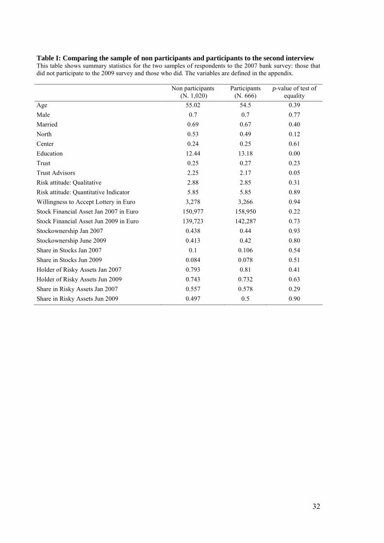
32

Table I: Comparing the sample of non participants and participants to the second interview This table shows summary statistics for the two samples of respondents to the 2007 bank survey: those that did not participate to the 2009 survey and those who did. The variables are defined in the appendix. Non participants

(N. 1,020) Participants

(N. 666) p-value of test of

equality Age 55.02 54.5 0.39 Male 0.7 0.7 0.77 Married 0.69 0.67 0.40 North 0.53 0.49 0.12 Center 0.24 0.25 0.61 Education 12.44 13.18 0.00 Trust 0.25 0.27 0.23 Trust Advisors 2.25 2.17 0.05 Risk attitude: Qualitative 2.88 2.85 0.31 Risk attitude: Quantitative Indicator 5.85 5.85 0.89 Willingness to Accept Lottery in Euro 3,278 3,266 0.94 Stock Financial Asset Jan 2007 in Euro 150,977 158,950 0.22 Stock Financial Asset Jun 2009 in Euro 139,723 142,287 0.73 Stockownership Jan 2007 0.438 0.44 0.93 Stockownership June 2009 0.413 0.42 0.80 Share in Stocks Jan 2007 0.1 0.106 0.54 Share in Stocks Jun 2009 0.084 0.078 0.51 Holder of Risky Assets Jan 2007 0.793 0.81 0.41 Holder of Risky Assets Jun 2009 0.743 0.732 0.63 Share in Risky Assets Jan 2007 0.557 0.578 0.29 Share in Risky Assets Jun 2009 0.497 0.5 0.90

33

Table II: Summary statistics of risk aversion measures, other variables and controls Panel A reports the summary statistics for the risk aversion measures. The qualitative risk aversion measure tries to elicit the investment objective of the respondent, offering them the choice among “Very high returns, even at the risk of a high probability of losing part of the principal;” A good return, but with an ok degree of safety of the principal;” “A ok return, with good degree of safety of the principal,” “Low returns, but no chance of losing the principal.” The responses are coded with integers from 1 to 4, with a higher score meaning a higher risk aversion. The quantitative risk-aversion measure tries to elicit the certainty equivalent for a gamble that delivers either 10,000 euro or zero with equal probability. We code the certainty equivalent with integers between 1 and 10, increasing in risk aversion. Change in cautiousness is obtained from answers to the following question asked in the 2009 survey: “After the stock market crash did you become more cautious and prudent in your investment decisions?” The possible answers are: “More or less like before”, “A bit more cautious”, “Much more cautious.” The variable change in cautiousness is zero if the response is “no change”, 1 if the response is “a bit more”, and 2 if it is “much more”. Panel B and C report the summary statistics for all the other variables defined in Table II and in the Appendix. Panel A. Risk aversion measures in 2007 and 2009 Quantitative measure (certainty

equivalent in euros) Qualitative measure

Mean Median Sd Mean Median Sd Level in 2007 4,027 4,000 3,254 2.87 3 0.72 Level in 2009 2,784 1,500 2,815 3.28 3 0.73 Change 2009/2007 -1,343 -1,000 3,994 0.42 0 0.81 Fraction of People with Increase in Risk Aversion 0.55 0.46

Fraction of People with Unchanged Risk Aversion 0.18 0.44

1- Fraction of People with a decrease in Risk Aversion 0.73 0.90

Panel B. Other variables: levels Mean Median Sd Male 0.70 1 0.46 Age 54.81 57 12.3 Educations (years) 12.73 13 4.25 Retired 0.33 0 0.47 Government Employee 0.33 0 0.47 Net Wealth 2007 (Log) 13.11 13.10 0.59 Net Wealth 2009 (Log) 13.05 13.03 0.64 Stock of Habits 2007 (Log) -0.07 -0.07 0.04 Stock of Habits 2009 (Log) -0.08 -0.07 0.16 Commitments 2007 (Log) 1.04 0.93 1.17 Commitments 2009 (Log) 1.43 1.19 1.66 Risky Asset Ownership 2007 0.65 1 0.48 Risky Asset Share 2007 0.27 0.20 28.5 Knightian Uncertainty 0.29 0 0.46 Trust Advisors 2007 3.78 4 0.91 Generalized Trust 2007 0.25 0 0.44

34

Panel C. Other variables: first differences Mean Median Sd Wealth 2007-2009, ΔLog -0.06 -0.051 0.27 Wealth 2008-2009, ΔLog -0.04 -0.005 0.20 Habit 2007-2009, ΔLog -0.003 -0.001 0.15 Commitments 2007-2009, ΔLog 0.40 0.16 1.16 Ownership Risky Assets -0.06 0 0.35 Share Risky Assets -0.04 0 0.24 Generalized Trust -0.08 0 0.52 Trust Advisors -0.23 0 1.11 Trust Stock Market 1.20 2 0.94 Stock Market Expected Return 819 47 6,626 Stock Market Return Uncertainty -144 50 5,674

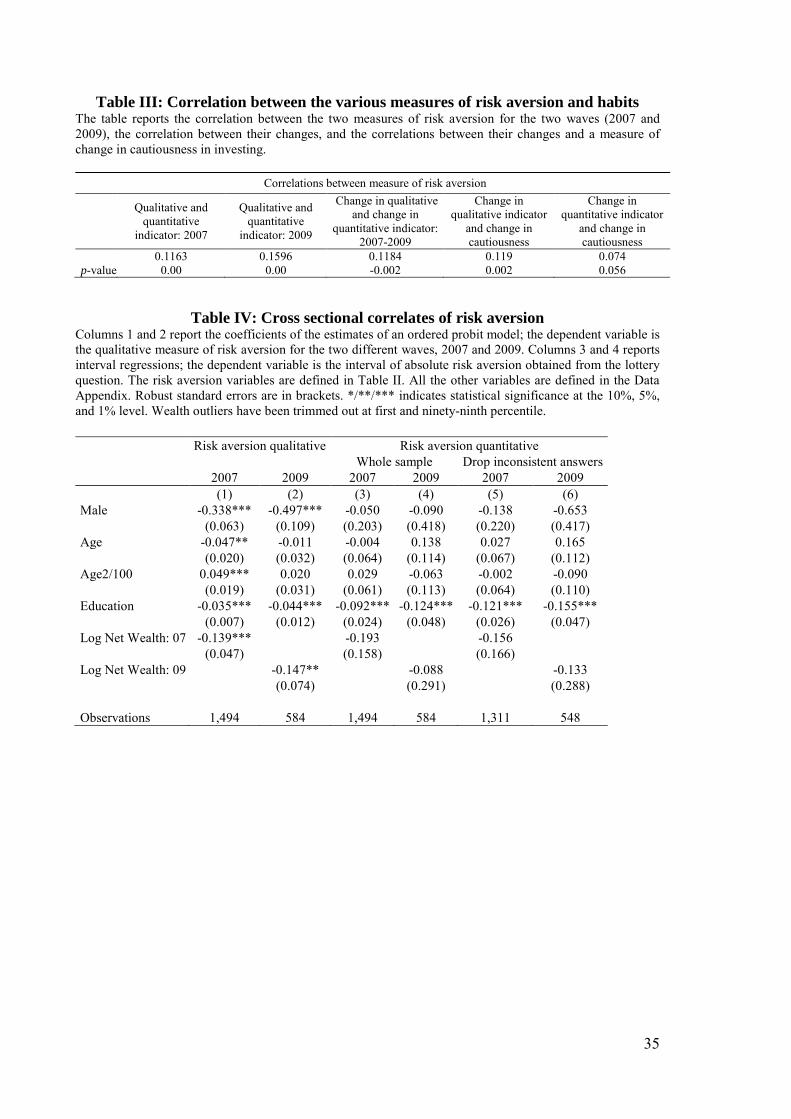
35

Table III: Correlation between the various measures of risk aversion and habits The table reports the correlation between the two measures of risk aversion for the two waves (2007 and 2009), the correlation between their changes, and the correlations between their changes and a measure of change in cautiousness in investing.

Correlations between measure of risk aversion Qualitative and

quantitative indicator: 2007

Qualitative and quantitative

indicator: 2009

Change in qualitative and change in

quantitative indicator: 2007-2009

Change in qualitative indicator

and change in cautiousness

Change in quantitative indicator

and change in cautiousness

0.1163 0.1596 0.1184 0.119 0.074 p-value 0.00 0.00 -0.002 0.002 0.056

Table IV: Cross sectional correlates of risk aversion Columns 1 and 2 report the coefficients of the estimates of an ordered probit model; the dependent variable is the qualitative measure of risk aversion for the two different waves, 2007 and 2009. Columns 3 and 4 reports interval regressions; the dependent variable is the interval of absolute risk aversion obtained from the lottery question. The risk aversion variables are defined in Table II. All the other variables are defined in the Data Appendix. Robust standard errors are in brackets. */**/*** indicates statistical significance at the 10%, 5%, and 1% level. Wealth outliers have been trimmed out at first and ninety-ninth percentile. Risk aversion qualitative Risk aversion quantitative

Whole sample Drop inconsistent answers

2007 2009 2007 2009 2007 2009

(1) (2) (3) (4) (5) (6) Male -0.338*** -0.497*** -0.050 -0.090 -0.138 -0.653

(0.063) (0.109) (0.203) (0.418) (0.220) (0.417)

Age -0.047** -0.011 -0.004 0.138 0.027 0.165

(0.020) (0.032) (0.064) (0.114) (0.067) (0.112)

Age2/100 0.049*** 0.020 0.029 -0.063 -0.002 -0.090

(0.019) (0.031) (0.061) (0.113) (0.064) (0.110)

Education -0.035*** -0.044*** -0.092*** -0.124*** -0.121*** -0.155***

(0.007) (0.012) (0.024) (0.048) (0.026) (0.047)

Log Net Wealth: 07 -0.139***

-0.193

-0.156

(0.047)

(0.158)

(0.166)

Log Net Wealth: 09

-0.147**

-0.088

-0.133

(0.074)

(0.291)

(0.288)

Observations 1,494 584 1,494 584 1,311 548

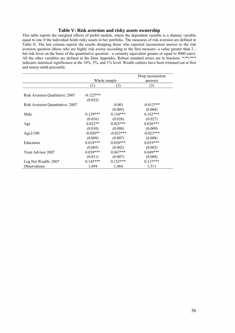
36

Table V: Risk aversion and risky assets ownership This table reports the marginal effects of probit models, where the dependent variable is a dummy variable equal to one if the individual holds risky assets in her portfolio. The measures of risk aversion are defined in Table II. The last column reports the results dropping those who reported inconsistent answer to the risk aversion question (those who are highly risk averse according to the first measure- a value greater than 2 - but risk lover on the basis of the quantitative question - a certainty equivalent greater or equal to 9000 euro). All the other variables are defined in the Data Appendix. Robust standard errors are in brackets. */**/*** indicates statistical significance at the 10%, 5%, and 1% level. Wealth outliers have been trimmed out at first and ninety-ninth percentile. Whole sample

Drop inconsistent answers

(1) (2) (3)

Risk Aversion Qualitative: 2007 -0.122***

(0.032)

Risk Aversion Quantitative: 2007

-0.001 -0.012***

(0.005) (0.004)

Male 0.129*** 0.154*** 0.162***

(0.016) (0.028) (0.027)

Age 0.022** 0.025*** 0.026***

(0.010) (0.008) (0.009)

Age2/100 -0.020** -0.023*** -0.023***

(0.009) (0.007) (0.008)

Education 0.018*** 0.020*** 0.019***

(0.005) (0.002) (0.002)

Trust Advisor 2007 0.039*** 0.047*** 0.049***

(0.011) (0.007) (0.008)

Log Net Wealth: 2007 0.145*** 0.152*** 0.137*** Observations 1,494 1,464 1,311

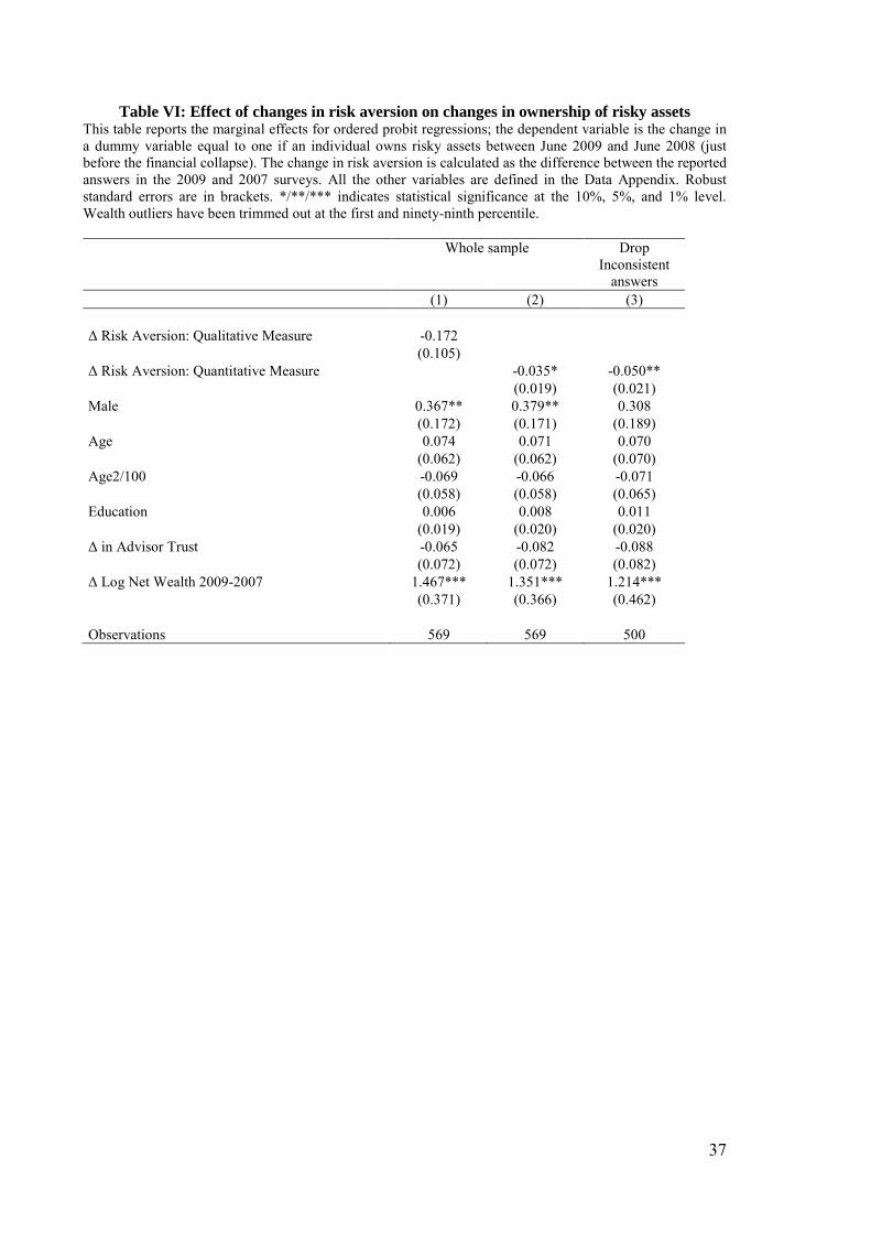
37

Table VI: Effect of changes in risk aversion on changes in ownership of risky assets This table reports the marginal effects for ordered probit regressions; the dependent variable is the change in a dummy variable equal to one if an individual owns risky assets between June 2009 and June 2008 (just before the financial collapse). The change in risk aversion is calculated as the difference between the reported answers in the 2009 and 2007 surveys. All the other variables are defined in the Data Appendix. Robust standard errors are in brackets. */**/*** indicates statistical significance at the 10%, 5%, and 1% level. Wealth outliers have been trimmed out at the first and ninety-ninth percentile.

Whole sample

Drop Inconsistent

answers (1) (2) (3)

Δ Risk Aversion: Qualitative Measure -0.172

(0.105)

Δ Risk Aversion: Quantitative Measure

-0.035* -0.050**

(0.019) (0.021)

Male 0.367** 0.379** 0.308

(0.172) (0.171) (0.189)

Age 0.074 0.071 0.070

(0.062) (0.062) (0.070)

Age2/100 -0.069 -0.066 -0.071

(0.058) (0.058) (0.065)

Education 0.006 0.008 0.011

(0.019) (0.020) (0.020)

Δ in Advisor Trust -0.065 -0.082 -0.088

(0.072) (0.072) (0.082)

Δ Log Net Wealth 2009-2007 1.467*** 1.351*** 1.214***

(0.371) (0.366) (0.462)

Observations 569 569 500

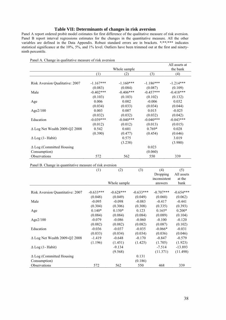
38

Table VII: Determinants of changes in risk aversion Panel A report ordered probit model estimates for first difference of the qualitative measure of risk aversion. Panel B report interval regressions estimates for the changes in the quantitative measure. All the other variables are defined in the Data Appendix. Robust standard errors are in brackets. */**/*** indicates statistical significance at the 10%, 5%, and 1% level. Outliers have been trimmed out at the first and ninety-ninth percentile.

Panel A. Change in qualitative measure of risk aversion

Whole sample

All assets at the bank

(1) (2) (3) (4)

Risk Aversion Qualitative: 2007 -1.167*** -1.160*** -1.186*** -1.214***

(0.083) (0.084) (0.087) (0.109)

Male -0.402*** -0.406*** -0.457*** -0.418***

(0.103) (0.103) (0.102) (0.132)

Age 0.006 0.002 -0.006 0.032

(0.034) (0.033) (0.034) (0.044)

Age2/100 0.003 0.007 0.015 -0.025

(0.032) (0.032) (0.032) (0.042)

Education -0.039*** -0.040*** -0.040*** -0.043***

(0.012) (0.012) (0.013) (0.015)

Δ Log Net Wealth 2009-Q2 2008 0.542 0.601 0.769* 0.028

(0.390) (0.477) (0.454) (0.646)

Δ Log (1- Habit)

0.575

3.019

(3.238)

(3.980)

Δ Log (Committed Housing

0.023 Consumption)

(0.060)

Observations 572 562 550 339

Panel B. Change in quantitative measure of risk aversion (1) (2) (3) (4) (5)

Whole sample

Dropping inconsistent

answers

All assets at the bank

Risk Aversion Quantitative: 2007 -0.633*** -0.628*** -0.633*** -0.707*** -0.654***

(0.048) (0.049) (0.049) (0.060) (0.062)

Male -0.095 -0.098 -0.083 -0.417 -0.441

(0.304) (0.306) (0.308) (0.335) (0.393)

Age 0.140* 0.150* 0.123 0.165* 0.200*

(0.084) (0.084) (0.084) (0.089) (0.104)

Age2/100 -0.079 -0.086 -0.060 -0.100 -0.120

(0.082) (0.082) (0.082) (0.087) (0.102)

Education -0.036 -0.037 -0.035 -0.066* -0.031

(0.033) (0.034) (0.034) (0.036) (0.046)

Δ Log Net Wealth 2009-Q2 2008 -1.419 -0.648 -0.170 -0.847 -0.579

(1.196) (1.451) (1.425) (1.705) (1.923)

Δ Log (1- Habit)

-9.134

-7.514 -13.893

(9.568)

(11.371) (11.498)

Δ Log (Committed Housing

0.131 Consumption)

(0.186)

Observations 572 562 550 468 339

39

Table VIII: The effect of uncertainty about future income and employment

The first column reports ordered probit model estimates; the dependent variable is the change in risk aversion measured with the answers to the qualitative question. The second column reports interval regression estimates; the dependent variable is the change in the quantitative measure of risk aversion. These measures are defined in Table II. All the other variables are defined in the Data Appendix. Robust standard errors are in brackets. */**/*** indicates statistical significance at the 10%, 5%, and 1% level. Wealth outliers have been trimmed out at the first and ninety-ninth percentile.

Change Risk Aversion: Qualitative

Change Risk Aversion: Quantitative

(1) (2) (3) (4)

Risk Aversion Qualitative: 2007 -1.163*** -1.153***

(0.084) (0.089)

Risk Aversion Quantitative: 2007

-0.630*** -0.645***

(0.049) (0.051)

Male -0.409*** -0.411*** -0.102 -0.150

(0.103) (0.113) (0.306) (0.331)

Age 0.006 -0.006 0.156* 0.153*

(0.034) (0.036) (0.089) (0.092)

Age2/100 0.001 0.015 -0.095 -0.083

(0.033) (0.035) (0.090) (0.095)

Education -0.039*** -0.042*** -0.036 -0.018

(0.012) (0.013) (0.034) (0.038)

Δ Log Net Wealth 2009-Q2 2008 0.599 0.471 -0.652 -1.631

(0.475) (0.541) (1.447) (1.576)

Δ Log (1- Habit) 0.577 0.909 -9.112 -7.267

(3.247) (3.356) (9.549) (9.799)

Retirees 0.079 -0.016 0.123 -0.048

(0.138) (0.146) (0.453) (0.484)

Government Employee

0.100

-0.302

(0.107)

(0.301)

Observations 562 525 562 525

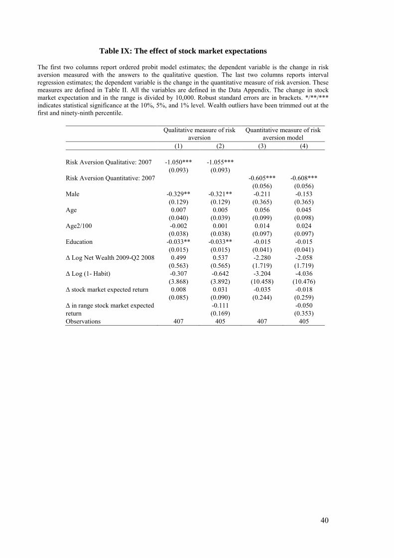
40

Table IX: The effect of stock market expectations

The first two columns report ordered probit model estimates; the dependent variable is the change in risk aversion measured with the answers to the qualitative question. The last two columns reports interval regression estimates; the dependent variable is the change in the quantitative measure of risk aversion. These measures are defined in Table II. All the variables are defined in the Data Appendix. The change in stock market expectation and in the range is divided by 10,000. Robust standard errors are in brackets. */**/*** indicates statistical significance at the 10%, 5%, and 1% level. Wealth outliers have been trimmed out at the first and ninety-ninth percentile.

Qualitative measure of risk aversion

Quantitative measure of risk aversion model

(1) (2) (3) (4) Risk Aversion Qualitative: 2007 -1.050*** -1.055***

(0.093) (0.093) Risk Aversion Quantitative: 2007

-0.605*** -0.608***

(0.056) (0.056)

Male -0.329** -0.321** -0.211 -0.153

(0.129) (0.129) (0.365) (0.365)

Age 0.007 0.005 0.056 0.045

(0.040) (0.039) (0.099) (0.098)

Age2/100 -0.002 0.001 0.014 0.024

(0.038) (0.038) (0.097) (0.097)

Education -0.033** -0.033** -0.015 -0.015

(0.015) (0.015) (0.041) (0.041)

Δ Log Net Wealth 2009-Q2 2008 0.499 0.537 -2.280 -2.058

(0.563) (0.565) (1.719) (1.719)

Δ Log (1- Habit) -0.307 -0.642 -3.204 -4.036

(3.868) (3.892) (10.458) (10.476)

Δ stock market expected return 0.008 0.031 -0.035 -0.018

(0.085) (0.090) (0.244) (0.259)

Δ in range stock market expected

-0.111

-0.050 return

(0.169)

(0.353)

Observations 407 405 407 405

41

Table X: The effect of trust and Knightian uncertainty

The first column reports ordered probit model estimates; the dependent variable is the change in risk aversion measured with the answers to the qualitative question. The second column reports interval regression estimates; the dependent variable is the change in the quantitative measure of risk aversion. These measures are defined in Table II. All the other variables are defined in the Data Appendix. Robust standard errors are in brackets. */**/*** indicates statistical significance at the 10%, 5%, and 1% level. Wealth outliers have been trimmed out at the first and ninety-ninth percentile.

Change Risk Aversion: Qualitative

Change Risk Aversion:

Quantitative (1) (2)

Risk Aversion Qualitative: 2007 -1.180***

(0.082)

Risk Aversion Quantitative: 2007

-0.625***

(0.049)

Male -0.290*** -0.017

(0.109) (0.313)

Age 0.009 0.151*

(0.033) (0.085)

Age2/100 -0.002 -0.089

(0.032) (0.083)

Education -0.035*** -0.036

(0.012) (0.034)

Δ Log Net Wealth 2009-Q2 2008 0.558 -0.664

(0.496) (1.437)

Δ Log (1- Habit) 0.848 -9.174

(3.286) (9.482)

Knightian Uncertainty 0.455*** 0.007

(0.107) (0.323)

Δ trust stock market -0.143*** -0.236*

(0.051) (0.140)

Observations 562 562

42

Table XI: Experimental evidence: comparison between the group of treated and untreated This table shows the summary statistics for treated and untreated subjects in the experiment run at Northwestern University and t-tests for the differences (last column). The risk aversion measures are elicited as described in Table II. The indicator for low risk investment is constructed from the qualitative question, setting it equal to 1 if the person chose “A OK return, with good degree of safety of my principal” or “Low returns, but no chance of losing my principal,” and zero otherwise. */**/*** indicates statistical significance at the 10%, 5%, and 1% level

Variable Obs. Tot. Mean treated Mean non-treated Difference

Risk Aversion Quantitative 207 1,802 2,474 -672** Risk Aversion Qualitative 210 2.54 2.41 0.13 Low Risk Investment 210 0.53 0.39 0.14* Sex 206 0.39 0.34 0.05 Age 203 19.77 19.83 -0.06 White 206 0.41 0.40 0.01 Income (Thousands of dollars) 210 111.68 120.96 - 9.28

43

Table XII: Fear and rebalancing The table reports the coefficients of regressions where the dependent variables is the flow of risky assets bought (positive) or sold (negative) over the period specified in each column scaled by the value of total financial assets at the end of August 2008, prior to the Lehman Brothers collapse. The risk aversion ratio is the ratio between the risk aversion before and after Lehman multiplied by the average risky share in 2007 (Z1); the post shock share is the risky share implied by the level of the risky asset price at various dates after the collapse of Lehman (Z2); its value depends on the drop in the price of risky assets between August the specified date. Total flow is the cumulative flow of total financial assets over the specified period. Robust standard errors are in brackets. */**/*** indicates statistical significance at the 10%, 5%, and 1% level. Outliers have been trimmed out at the first and ninety-ninth percentile. Rebalancing interval Oct 08 Oct 08 Oct 08 Oct 08 Oct 08 Oct 08 VARIABLES /Jan 09 /Feb 09 /Mar 09 /Apr 09 /May 09

(1) (2) (3) (4) (5) (6)

Risk aversion ratio (Z1) 0.035* 0.035* 0.025 0.056** 0.067** 0.058*

(0.018) (0.020) (0.021) (0.028) (0.030) (0.033)

Post shock share: Sep 08 (Z2) -0.057***

(0.021)

Post shock share: Oct 08 (Z2)

-0.046**

(0.023)

Post shock share: Nov 08 (Z2)

-0.041*

(0.025)

Post shock share: Dec 08 (Z2)

-0.082***

(0.030)

Post shock share: Jan 08 (Z2)

-0.104***

(0.033)

Post shock share: Feb 08 (Z2)

-0.089**

(0.036)

Male -0.005 -0.020 -0.026* -0.029* -0.036** -0.031*

(0.010) (0.013) (0.014) (0.015) (0.016) (0.017)

Age 0.007** -0.002 0.002 -0.001 -0.001 -0.003

(0.003) (0.006) (0.006) (0.006) (0.006) (0.007)

Age2/100 -0.006** 0.001 -0.002 0.001 0.001 0.004

(0.003) (0.005) (0.006) (0.006) (0.006) (0.006)

Education 0.001 0.001 0.002 0.002 0.002 0.002

(0.001) (0.001) (0.002) (0.002) (0.002) (0.002)

Δ Log Net Wealth 2009-Q2 2008 0.220*** 0.312*** 0.307*** 0.337*** 0.370*** 0.449***

(0.072) (0.087) (0.089) (0.087) (0.089) (0.100)

Tot flow Oct 08/Dec 08 -0.000

(0.000)

Tot flow Oct 08/Jan 08

0.001

(0.001)

Tot flow Oct 08/Feb 08

0.002

(0.002)

Tot flow Oct 08/Mar 09

0.005

(0.005)

Tot flow Oct 08/Apr 09

0.013

(0.008)

Tot flow Oct 08/May 09

0.000

(0.004)

Observations 502 502 502 502 502 502 R-squared 0.085 0.098 0.089 0.100 0.126 0.122

44

Data Appendix

A.1 Variables Definition

Habit stock: is the ratio of imputed non durable consumption and the stock of household total net worth, defined as the sum of housing wealth and financial assets net of total outstanding debt.

House consumption commitment: is the ratio of housing value divided by the stock of financial assets.

Change stock market expectations: investors were asked to report the distribution of stock returns one year ahead. Specifically they were asked to state what he thinks would be the value of a 10,000 euro investment in a fully diversified stock mutual after 12 months. They were asked to report the minimum value first, then the maximum. Subsequently they were asked to report the probability that the value of the stock by the end of the 12 months is above the mid-point of the reported support. Under some assumptions about the shape of the distribution, this parsimonious information allows computing the subjective mean and variance of stock market returns. Stock market expectation is the first moment of the distribution. We have computed these moments assuming the distribution is uniform but results are the same assuming it is triangular. The change in stock market expectation is the difference between the two surveys.

Range in stock market beliefs: is the difference between the maximum and minimum value of the investment reported in the answers to the previous question. The change in the range is the difference between the two surveys.

Knightian uncertainty: a dummy equal to 1 if in 2007 the investor is able to answer the question about the probability distribution of stock prices but is unable to in 2009; zero otherwise.

Change in trust in stock market: answers to the question asked in the 2009 survey: “How is the trust towards the stock market changes between September 2008 and today? a) increased a lot; increased a bit; c) unchanged; d) decreased a bit; decreased a lot. Answers are coded with integers between 1 and 5 with higher numbers reflecting increased trust. Trust advisor: answers to the question asked in both surveys: “Overall, how much trust do you have in your bank advisor or financial broker concerning your financial investments?” with the answers ranging from 1 (I trust a lot) to 5(No trust at all). We have recoded them so that the variable is increasing in trust. A.2. The 2007 survey The survey data used draw on a sample of Italian clients of a large Italian bank. The survey was conducted between June and September 2007 and elicited detailed financial and demographic information on a sample of 1,686 individuals with a checking account in one of the branches of the bank. The eligible population of customers excludes customers under 20 and over 80, and customers with assets of less than 10,000 Euros with the bank. The sampled population size is around 1.3 million customers. The survey was aimed at acquiring information on the behavior and expectations of the bank’s customers and focused on multi-banking, attitude towards saving and

45

investing, financial literacy and propensity for risk, pensions and need for insurance. The sample is stratified according to three criteria: geographical area, city size, financial wealth, and it explicitly over-samples rich clients. In particular, only clients with at least €10,000 of financial wealth at the bank at the end of 2006 are included in the sample. An important feature of the survey is that only individual retail investors at this particular bank were sampled. The survey, however, also contains detailed information on the spouse, if present. Financial variables are elicited for both respondents and households. In the paper, demographic variables refer to the household head (even if different from the respondent), and economic variables (real and financial assets) to the household, not to the individual investor. The survey contains detailed information on ownership of real and financial assets, and amounts invested. For real assets, the bank reports separate data on primary residence, investment real estate, land, business wealth, and debt (distinguished between mortgage and other debt). Real asset amounts are elicited without use of bracketing. The sampling scheme is similar to that of the Bank of Italy Survey of Household Income and Wealth (SHIW). The population is stratified along two criteria: geographical area of residence (North-East, North-West, Central and Southern Italy) and wealth held with the bank as of June 30 2006. The sample size is 1,686 customers, of whom 1,580 are from the retail bank belonging to the group, and 106 from the private bank (which targets upper tier customers). The survey was administered between May 1 and September 30 of 2007 by a leading Italian polling agency, which also conducts the SHIW for the Bank of Italy. Most interviewers had substantial experience of administering the SHIW, which is likely to increase the quality of the data. The survey was piloted in the first quarter of 2007, and the Computer Assisted Personal Interview methodology was employed for all interviews. To overcome some of the problems arising from non-responses, the sample was balanced ex-post with respect to the true distribution of assets, area of residence, city size, gender, age and education of the eligible population. The questionnaire comprises 9 sections. Sections A and B refer, respectively, to respondent and household demographic and occupation variables. Section C focuses on saving, investment and financial risk. Section D asks detailed questions about financial wealth and portfolio allocation, and Section E enquires about consumer debt and mortgages. By design, Sections A, B, D and E allow a perfect matching with the SHIW questionnaire. Questions on real estate and entrepreneurial activities are included in Section F. Section G contains questions on subjective expectations, and section H focuses on insurance and private pension funds. The last two sections ask about income and expectations and need for insurance and pension products. As shown in Table 1A, compared with the Italian population, as surveyed by the 2006 Bank of Italy SHIW, bank customers are older, more educated, less likely to work in the manufacturing sector, and more likely to live in the North.

Table A1: Bank survey – SHIW comparison Bank survey SHIW

Highest income earner SHIW

Bank account holder Gender Male 0.69 0.69 0.71 Female 0.31 0.31 0.29 Age Up to 30 0.04 0.06 0.06 31 to 40 0.18 0.19 0.20 41 to 50 0.22 0.22 0.22 51 to 65 0.36 0.24 0.24 Over 65 0.20 0.29 0.27 Education Elementary School 0.10 0.27 0.22 Middle School 0.29 0.36 0.37 High School 0.41 0.27 0.30 University Degree 0.20 0.10 0.10

46

Sector of activity Agriculture 0.03 0.03 0.03 Industry 0.13 0.21 0.23 Public Administration

0.19 0.15 0.17 Other sectors 0.30 0.19 0.20 Not employed 0.35 0.40 0.37 Household Size 1 member 0.21 0.25 0.23 2 members 0.29 0.28 0.29 3 members 0.26 0.21 0.22 4 members 0.20 0.18 0.19 5 or more members 0.04 0.07 0.06 Geographical Area Northern Italy 0.73 0.48 0.52 Central Italy 0.14 0.20 0.21 South and Islands 0.13 0.32 0.27

Note: The table compares sample means of selected demographic variables in the bank survey and 2006 SHIW. Means are computed using sample weights. A3. The administrative bank survey data We complement the 2007 survey with administrative data on assets’ stocks and net flows that we use to compute measures of wealth and changes and portfolio allocation before and after the crisis. The bank administrative dataset contains information on the stocks and on the net flows of 26 assets categories that investors have at the bank1. These data are available at monthly frequency for 35 months beginning in December 2006. The administrative data reports this information for the investors that actually participated in the 2007 survey and can indeed be matched with the 2007 bank survey data. Notice that the administrative data form a balanced panel. We use these data to obtain measures of people financial wealth and portfolio compositions at various points in time before and after the financial crisis. A4. The 2009 telephone survey In June 2009, the same company that fielded the 2007 bank survey re-contacted the respondents to the 2007 survey asking for their willingness to participate in a short telephone interview. Out of 1,686 contacts, 666 completed the telephone interview.

The questionnaire was designed to ask a set of select questions that were asked in the 2007 using exactly the same wording. In particular we asked a qualitative risk aversion question, a hypothetical risky lottery question, a generalized trust and trust in own bank question and a question eliciting the probability distribution of stock market returns. In addition, a few other questions were asked that were not asked in the 2007 survey. At the beginning of the interview the interviewer asked a number of demographic characteristics in order to make sure that the respondent was the same who participated in the 2007 interview.

1 The list includes: checking accounts, time deposits, deposit certificates, stock mutual funds, money market mutual funds, bond mutual funds, other mutual funds, ETF, linked funds, Italian stocks, foreign stocks, unit linked insurance, recurrent premium, unit linked insurance, one shot premium, stock market index, life insurance recurrent premium, life insurance one shot premium, pension funds, T-bills short term, T-bonds, indexed T-bonds, other T-bills, managed accounts, own bank bonds, corporate bonds Italy, corporate bonds foreign, other bonds.

47

0.0

5.1

.15

fract

ion

-10 -5 0 5 10change in lottery based risk aversion indicator

0.1

.2.3

.4.5

fract

ion

-2 0 2 4dproprisk

A5. Additional analysis This section complements some of the figures and Tables in text and provides additional statistics and analysis.

Figure A1. Frequency distribution of the change in risk aversion indicators 2009 and 2007 The figure shows the distribution of the first difference of the risk aversion indicators between 2009 and 2007. Panel A used the whole sample; Panel B and C reports the distribution of the change accounting for censoring (Panel B) and dropping inconsistent answers across the two questions (Panel C)

A. Whole sample

B. Accounting for censoring

C. Dropping the inconsistent and accounting for censoring

0.1

.2.3

.4.5

fra

ctio

n

-2 0 2 4dproprisk

0.0

5.1

.15

frac

tion

-10 -5 0 5 10change in lottery based risk aversion indicator

0.1

.2.3

.4fr

act

ion

-4 -2 0 2 4Change in qualitative risk aversion indicator

0.0

5.1

.15

.2fr

act

ion

-10 -5 0 5 10Change in lottery based risk aversion indicator

48

Table A.2: Correlation between the various measures of risk aversion and habits The table reports the correlation between the measures of habit in 2007 and 2009. Habit is the ratio of imputed non- durable consumption and the stock of household total net worth, the sum of housing wealth and financial assets net of total outstanding debt; house consumption commitment is the ratio of housing value divided by the stock of financial assets.

Correlation between Log (1-habit) and Log (house consumption

commitment) 2007

Correlation between Log (1-habit) and Log (house consumption

commitment) 2009 -0.310 -0.214

p-value 0.00 0.00

Table A.3: Risk aversion and share of risky assets This table presents robustness regressions corresponding to Table V in the paper. The table reports the coefficients of tobit regressions, where the dependent variable is the share of risky assets over the entire portfolio. The measures of risk aversion are defined as in Table II. The last column reports the results dropping those who reported inconsistent answer to the risk aversion question (those who are highly risk averse according to the first measure- a value greater than 2 - but risk lover on the basis of the quantitative question - a certainty equivalent greater or equal to 9000 euro). All the other variables are defined in the Data Appendix. Robust standard errors are in brackets. */**/*** indicates statistical significance at the 10%, 5%, and 1% level. Wealth outliers have been trimmed out at first and ninety-ninth percentile.

Whole sample

Drop inconsistent

answers (1) (2) (3) Risk Aversion Qualitative: 2007 -0.141***

(0.021) Risk Aversion Quantitative: 2007

-0.003 -0.013***

(0.005) (0.004)

Male 0.084*** 0.115*** 0.111***

(0.018) (0.026) (0.028)

Age 0.018** 0.022** 0.023**

(0.009) (0.009) (0.010)

Age2/100 -0.015** -0.020** -0.021**

(0.008) (0.009) (0.009)

Education 0.012*** 0.015*** 0.013***

(0.004) (0.002) (0.002)

Trust Advisor 2007 0.023** 0.032*** 0.033***

(0.011) (0.008) (0.009)

Log Net Wealth: 2007 0.107*** 0.121*** 0.109***

(0.008) (0.029) (0.025)

Observations 1,494 1,494 1,311

49

Table A.4: Effect of changes in risk aversion on the share of risky assets This table presents robustness tests corresponding to Table VI in the paper. The table reports the coefficients of OLS regressions, where the dependent variable is the change in the share of risky assets owned between June 2008 and June 2009. The change in risk aversion is calculated as the difference between the reported answers in the 2009 and 2007 surveys. All the other variables are defined in the Data Appendix. Robust standard errors are in brackets. */**/*** indicates statistical significance at the 10%, 5%, and 1% level. Wealth outliers have been trimmed out at the first and ninety-ninth percentile.

Whole sample

Drop inconsistent answers

(1) (2) (3)

Δ Risk Aversion: Qualitative Measure -0.009

(0.013)

Δ Risk Aversion: Quantitative Measure

-0.006** -0.006**

(0.002) (0.003)

Male -0.019 -0.016 -0.031

(0.023) (0.023) (0.023)

Age -0.000 0.001 -0.002

(0.009) (0.008) (0.009)

Age2/100 -0.000 -0.001 0.001

(0.008) (0.008) (0.008)

Education -0.002 -0.001 -0.001

(0.002) (0.002) (0.002)

Δ in Advisor Trust -0.007 -0.009 -0.014

(0.009) (0.009) (0.010)

Δ Log Net Wealth 2009-2007 0.133* 0.121* 0.077

(0.069) (0.068) (0.074)

Initial Share in Risky Assets -0.167*** -0.163*** -0.151***

(0.023) (0.023) (0.023)

Observations 569 569 500 R-squared 0.090 0.097 0.094

Table A.5: Transition matrix of the qualitative measure of risk aversion 2007-2009 This table reports the transition matrix of the qualitative measure of risk aversion, between 2007 and 2009. The indicator is defined in Table II.

Risk aversion: Qualitative Indicator 2009

Risk aversion: Qualitative Indicator 2007

High risk/high

return

Moderate risk/medium

return

Small risk/ some return

No risk/ low

return Total

High Risk/High Return 2 6 2 2 12 Moderate Risk/Medium Return 4 38 95 44 181

Small Risk/Some Return 2 33 172 160 367 No Risk/Low Return 1 5 22 78 106 Total 9 82 291 284 666

50

Table A.6: Transition matrix of the quantitative measure of risk aversion 2007-2009 Panel A maps absolute risk aversion (ARA) intervals and certainty equivalent into risk categories; the ARA interval is the interval of the degree of absolute risk aversion (x1, 000) implicit in the answers to the lottery questions. Panel B reports the transition matrix of the quantitative measure of risk aversion, between the 2007 and 2009. The measure is illustrated in Table II. Values for 2007 are reported in rows, while those for 2009 are displayed in columns. For the open interval of the lowest (respectively, highest) risk aversion category the lower (respectively higher) bound is not observed and is denoted with a “.” Panel A. ARA Interval and Certainty equivalent mapped into Risk categories

Risk aversion category 1 2 3 4 5 6 7 8 9 10 Certainty equivalent >9000 9000 7000 5500 5000 4000 3000 1500 500 100 ARA interval Lower bound . -0.692 0.180 0.04 0.00 0.082 0.18 0.446 1.386 6.932 Upper bound -0.692 0.180 0.04 0.00 0.082 0.18 0.446 1.386 6.932 .

Panel B. Transition matrix of the quantitative measure of risk aversion indicator between the 2007 and 2009 Risk aversion 2009 Risk aversion 2007 1 2 3 4 5 6 7 8 9 10 Total 1 5 2 3 0 8 4 8 11 3 22 66 2 6 3 5 3 14 4 10 7 4 14 70 3 4 2 2 1 11 1 5 10 4 13 53 4 1 0 0 1 1 1 4 2 1 2 13 5 5 3 3 2 18 3 21 8 3 29 95 6 4 2 0 0 4 2 9 8 3 13 45 7 4 0 2 3 16 5 21 23 6 23 103 8 4 0 1 0 8 2 11 19 8 16 69 9 4 2 1 1 5 1 6 10 8 12 50 10 5 2 5 1 6 1 13 17 11 41 102

Total 42 16 22 12 91 24 108 115 51 185 666

51

Table A.7: Determinants of changes in risk aversion: non-linear effects This table reports robustness analysis for Table VII in the text. The first two columns report ordered probit model estimates for first difference of the qualitative measure of risk aversion. The last two columns report interval regressions estimates for the changes in the quantitative measure. All the other variables are defined in the Data Appendix. Robust standard errors are in brackets. */**/*** indicates statistical significance at the 10%, 5%, and 1% level. Outliers have been trimmed out at the first and ninety-ninth percentile.

Change in Qualitative Indicator of

Risk Aversion

Change in Quantitative Indicator of

Risk Aversion

Risk Aversion Qualitative: 2007 -1.168***

(0.084)

Risk Aversion Quantitative: 2007

-0.631***

(0.049)

Male -0.405*** -0.105

(0.103) (0.304)

Age 0.005 0.134

(0.034) (0.083)

Age2/100 0.004 -0.074

(0.032) (0.081)

Education -0.039*** -0.034

(0.012) (0.033)

Δ Log Net Wealth 2009-Q2 2008 0.134 -3.078*

(0.562) (1.684)

(Δ Log Net Wealth 2009-Q2 2008) 2 -1.153 -4.588

(1.167) (3.989)

Observations 572 572

52

Table A.8: Experimental evidence The table reports estimates of the effect of the treatment on subjects risk aversion. In columns 1 and 2 the dependent variable is the quantitative measure of risk aversion measured by certainty equivalent in columns 3 and 4 the left hand side is the qualitative measure of risk aversion; and in columns 5 and 6 a dummy variable equal to 1 if low risk investments are chosen. Columns 1-4 report results from OLS regressions, while columns 5-6 marginal effects from probit estimates. The variable “Treated” is a dummy variable equal to one if the individual was treated by showing him the video, and zero otherwise. All the other variables are defined in Table II, XVI and in the Data Appendix. Robust standard errors are in brackets. */**/*** indicates statistical significance at the 10%, 5%, and 1% level

Risk Aversion Quantitative Risk Aversion Qualitative Prob. Choose Low Risk Inv.

(1) (2) (3) (4) (5) (6) Treated -671.739** -637.516** 0.128 0.120 0.135** 0.143** (300.210) (300.136) (0.080) (0.080) (0.069) (0.070) Gender 347.001 -0.185** -0.165** (313.255) (0.080) (0.071) Income (Million -980.767 -0.193 0.200 dollars) (1,032.326) (0.397) (0.303) Constant 2,473.913*** 2,415.522*** 2.409*** 2.510*** (214.947) (293.520) (0.055) (0.078) Observations 207 203 210 206 210 206 R-squared 0.023 0.028 0.012 0.036 0.013 0.031