FEDERAL RESERVE BANK OF SAN FRANCISCO

WORKING PAPER SERIES

The views in this paper are solely the responsibility of the authors and should not be interpreted as reflecting the views of the Federal Reserve Bank of San Francisco or the Board of Governors of the Federal Reserve System.

Time-Varying U.S. Inflation Dynamics and the New Keynesian Phillips Curve

Kevin J. Lansing Federal Reserve Bank of San Francisco

August 2008

Working Paper 2006-15 http://www.frbsf.org/publications/economics/papers/2006/wp06-15bk.pdf

Time-Varying U.S. In�ation Dynamicsand the New Keynesian Phillips Curve�

Kevin J. Lansingy

Federal Reserve Bank of San Francisco

August 12, 2008

Abstract

This paper introduces a form of boundedly-rational in�ation expectations in the NewKeynesian Phillips curve. The representative agent is assumed to behave as an econome-trician, employing a time series model for in�ation that allows for both permanent andtemporary shocks. The near-unity coe¢ cient on expected in�ation in the Phillips curvecauses the agent�s perception of a unit root in in�ation to become close to self-ful�lling.In a �consistent expectations equilibrium,�the value of the Kalman gain parameter in theagent�s forecast rule is pinned down using the observed autocorrelation of in�ation changes.The forecast errors observed by the agent are close to white noise, making it di¢ cult forthe agent to detect a misspeci�cation of the forecast rule. I show that this simple model ofin�ation expectations can generate time-varying persistence and volatility that is broadlysimilar to that observed in long-run U.S. data. Model-based values for expected in�ationtrack well with movements in survey-based measures of U.S. expected in�ation. In nu-merical simulations, the model can generate pronounced low-frequency swings in the levelof in�ation that are driven solely by expectational feedback, not by changes in monetarypolicy.

Keywords: In�ation Expectations, Phillips Curve, Time-Varying Persistence & Volatility.

JEL Classi�cation: E31, E37.

�Forthcoming, Review of Economic Dynamics. For helpful comments and suggestions, I thank Marc Gian-noni, Cars Hommes, John Roberts, Karl Whelan, seminar participants at the University of Amsterdam, NorgesBank, and other economic conferences. I also thank an anonymous referee and an associate editor for thoughtfulsuggestions that improved the paper.

y Research Department, Federal Reserve Bank of San Francisco, P.O. Box 7702, San Francisco,CA 94120-7702, (415) 974-2393, FAX: (415) 977-4031, email: kevin.j.lansing@sf.frb.org, homepage:www.frbsf.org/economics/economists/klansing.html

1 Introduction

1.1 Overview

The New Keynesian Phillips Curve (NKPC) is derived most straightforwardly from Calvo�s

(1983) model of sticky price adjustment. Numerous researchers have criticized the fully-

rational NKPC on grounds that a reasonably parameterized version fails to capture important

features of post-World War II U.S. data, namely, high levels of in�ation persistence and the

delayed and gradual response of in�ation to unanticipated monetary policy shocks.1 Other

researchers have argued that the appropriate inclusion of exogenous stochastic driving variables

that re�ect changes in monetary policy can improve the empirical performance of the fully-

rational NKPC.2

This paper introduces a form of boundedly-rational in�ation expectations in the NKPC for

an economy where all monetary policy variables are held constant. The representative agent

is assumed to behave as an econometrician, employing a time series model for in�ation that

allows for both permanent and temporary shocks. The agent�s perceived optimal forecast rule

is de�ned by the Kalman �lter. I show that the perceived optimal value of the Kalman gain

parameter assigned to the last observed in�ation rate is given by the �xed point of a nonlinear

map that relates the gain parameter to the observed autocorrelation of in�ation changes. By

computing the value of the autocorrelation coe¢ cient, the agent can identify the �signal-to-

noise ratio,�which measures the relative variances of the perceived permanent and temporary

shocks to in�ation. A higher signal-to-noise ratio calls for a higher Kalman gain parameter

which, in turn, places more weight on recent in�ation data in the agent�s forecast rule. In a

�consistent expectations equilibrium,� the forecast errors observed by the agent are close to

white noise, making it di¢ cult for the agent to detect a misspeci�cation of the forecast rule.3

Moreover, from the individual agent�s perspective, switching to a fundamentals-based in�ation

forecast (which makes use of the output gap or real marginal cost) would appear to reduce

forecast accuracy, so there is no incentive to switch. Intuitively, the equilibrium exploits the

fact that expected in�ation enters the NKPC with a near-unity coe¢ cient. This feature causes

the agent�s perception of a unit root in in�ation to become close to self-ful�lling.

The model allows for either a constant gain or a variable gain, depending on the length

of the sample period used by the agent to identify the signal-to-noise ratio from observed

in�ation data. As the sample period becomes in�nitely long, the equilibrium yields a constant

gain. A rolling sample period yields a variable gain. From the agent�s perspective, the use

of a variable Kalman gain is justi�ed by perceived movements in the signal-to-noise ratio.

1See, for example, Roberts (1997, 2005), Fuhrer (1997, 2006), Mankiw (2001), Estrella and Fuhrer (2002),and Rudd and Whelan (2005a, 2007).

2See, for example, Kozicki and Tinsley (2002, 2005), Ireland (2007), and Cogley and Sbordone (2008).3This boundedly-rational equilibrium concept was developed by Hommes and Sorger (1998). A closely-

related concept is the �restricted perceptions equilibrium�described by Evans and Honkopohja (2001, Chapter13).

1

In the variable-gain version of the model, the nonlinear law of motion for in�ation generates

time-varying persistence and volatility that is broadly similar to that observed in long-run

U.S. data.

The model�s methodology for identifying the signal-to-noise ratio can be applied directly

to U.S. in�ation data. The identi�ed U.S. signal-to-noise ratio exhibits an upward drift during

the 1970s, followed by downward drift from the mid-1990s onwards. The downward drifting

ratio over the last decade indicates a reduced likelihood of a permanent shift, either upwards

or downwards, in the Fed�s in�ation target. This evidence is consistent with the idea of

�well-anchored in�ation expectations�in describing the recent environment (see, for example,

Williams 2006). The identi�ed signal-to-noise ratio in U.S. data might therefore be viewed as

an inverse measure of the Fed�s credibility for maintaining a constant in�ation target. In the

consistent expectations framework, the agent�s in�ation forecast is an exponentially-weighted

moving average of past observed in�ation rates. This feature tracks well with movements in

survey-based measures of U.S. expected in�ation.

The driving variable for in�ation in the model can be interpreted as either the output gap or

real marginal cost. Monetary policy enters the model implicitly through two channels: (i) the

steady-state in�ation rate around which the NKPC is log-linearized� maintained here at zero,

or (ii) the parameters that govern the exogenous stochastic process for the driving variable.

All policy-dependent parameters are held constant throughout the analysis. Interestingly, the

model can generate pronounced low-frequency swings in the level of in�ation that are driven

solely by expectational feedback, not by changes in monetary policy. The low-frequency swings

derive from the near-random walk behavior of in�ation under consistent expectations. From

the agent�s perspective, the observed low-frequency swings justify the use of a forecast rule

that allows for permanent shocks. This aspect of the model bears similarity to the �optimal

misspeci�ed beliefs�concept described by Sargent (1999, Chapter 6).

Klein (1978) and Barsky (1987) were among the �rst to call attention to the dramatic

changes in in�ation persistence in long-run U.S. data. Barsky (p. 3) noted that �In�ation

evolved from essentially a white noise process in the pre-World War I years, to a highly

persistent, non-stationary ARIMA process in the post-1960 period.�More recently, Cogley

and Sargent (2002, 2005) employ vector autoregressions that allow for drifting coe¢ cients

and stochastic volatility to document the evolving nature of U.S. in�ation dynamics in post-

World War II data. Their methodology identi�es a positive correlation between measures of

persistence, volatility, and the level of in�ation in post-World War II data. Simple 20-year

rolling summary statistics con�rm these basic �ndings. As a caveat, it should be noted that

�ndings of time-varying in�ation persistence in recent data are not universal. Pivetta and Reis

(2007) argue that the wide con�dence intervals around measures of in�ation persistence do

not allow one to reject the hypothesis of no change in persistence since 1965. These authors

do �nd robust evidence of a change in in�ation volatility, however.

Shifts in monetary policy are one candidate for explaining changes in in�ation dynamics.

2

Both Klein (1978) and Barsky (1987) attribute the change in in�ation persistence after World

War I to the abandonment of the classical gold standard. A gold standard can be viewed as a

price-level targeting regime. Under an in�ation-targeting regime, shifts in the central bank�s

in�ation target (which determines the trend in�ation rate) can distort standard measures

of persistence and volatility. For this reason, measures of persistence and volatility should

be conditioned on an estimate of trend in�ation.4 In computing the 20-year rolling summary

statistics, I control for shifts in trend in�ation by �rst extracting the low-frequency component

of U.S. in�ation. Detrended in�ation continues to exhibit time-varying patterns of persistence

and volatility, even during periods of seemingly-unchanged monetary policy, such as the sample

period since 1995. Such observations suggest that U.S. in�ation is driven by a number of

di¤erent nonlinearities, not just those attributable to policy regime shifts.

1.2 Related Literature

The consideration of boundedly-rational in�ation expectations is motivated by empirical evi-

dence. Survey-based measures of U.S. in�ation expectations tend to systematically underpre-

dict actual in�ation in the sample period prior to October 1979 and systematically overpredict

it thereafter. Rational expectations would not give rise to a sustained sequence of one-sided

forecast errors. Roberts (1997), Carroll (2003), Mankiw, Reis, and Wolfers (2004), and Branch

(2004) all �nd evidence that survey-based measures of U.S. in�ation expectations do not make

the most e¢ cient use of available information.

The boundedly-rational form of expectations used here is similar to that explored by Evans

and Ramey (2006) in the context of the Lucas (1973) monetary policy model. In their frame-

work, the value of the gain parameter is pinned down using a Nash equilibrium concept.5

An empirical study by Ball (2000) allows for a switch between two forms of �near-rational�

forecast rules to help account for the dramatic change in U.S. in�ation persistence identi�ed

by Klein (1978) and Barsky (1987). In Ball�s framework, the switch between forecast rules is

imposed within the model; it is not an endogenous response to an actual or perceived shift in

fundamentals.

Orphanides and Williams (2005) and Milani (2005) introduce in�ation persistence in the

form of constant-gain learning in models where the underlying fundamentals do not shift. The

representative agent�s perceived law of motion for in�ation is an AR(1) process with parameters

that are perpetually re-estimated using recent data. Unlike here, the constant gain used in the

learning algorithm is a free parameter that is calibrated rather than endogenized within the

model itself. In the learning model of Erceg and Levin (2003), the value of the gain parameter

is estimated by minimizing the squared deviations between the model�s in�ation expectations

4This point has been emphasized by Kozicki and Tinsley (2002), Levin and Piger (2004), and Marques(2004), among others.

5The use of a Nash equilibrium to determine the gain was �rst demonstrated by Evans and Honkopohja(1993).

3

and survey-based U.S. in�ation expectations.

Research that examines the links between exogenous policy rule shifts and in�ation dynam-

ics includes Boivin and Giannoni (2006), Roberts (2006), and Cecchetti et al. (2007). Papers

by Kozicki and Tinsley (2002, 2005), Ireland (2007), and Cogley and Sbordone (2008) show

that the empirical performance of the fully-rational NKPC can be improved by introducing

a highly persistent, exogenous stochastic process for the central bank�s in�ation target. It

remains unclear, however, why an optimizing central bank would wish to adopt such a process

for the in�ation target.6 Moreover, in order to account for the time-varying dynamic prop-

erties of detrended U.S. in�ation, these models would need to incorporate exogenous shifts

in other parameters of the central bank�s policy rule. The approach taken here is to develop

a model that abstracts from actual shifts in the central bank�s in�ation target or any other

aspect of monetary policy. The model simulations are compared to U.S. data on the basis

of detrended in�ation behavior� analogous to the methodology employed in the real business

cycle literature. The main message of the paper is that expectational feedback can be an

important driving force for in�ation dynamics.

2 Time-Varying Persistence and Volatility in U.S. In�ation

Figure 1 provides evidence of time-varying persistence and volatility in U.S. in�ation data.

The left-side panels plot the data and 20-year rolling summary statistics for CPI in�ation

from 1871.Q1 to 2004.Q4. The right-side panels plot the same information for GDP price

in�ation from 1949.Q1 to 2004.Q4.7 The 20-year rolling summary statistics are computed for

both the raw and detrended in�ation series. Detrending is a way to control for shifts in the

central bank�s in�ation target that may have occurred over time.8

[Figure 1 about here]

Panel 1a illustrates the dramatic di¤erence in the behavior of pre- and post-World War I

in�ation noted by Klein (1978) and Barsky (1987). The simple measure of persistence used

6 In Ireland (2007), the law of motion for the in�ation target is a geometric random walk. Exogenous shockscan permanently shift the target by amounts that are determined by exogenous monetary policy coe¢ cients.

7The annualized 1-quarter in�ation rate is given by 4 log (Pt=Pt�1) ; where Pt is the relevant price in-dex. The quarterly CPI data were constructed by averaging monthly CPI data obtained from RobertShiller�s website: http://www.econ.yale.edu/~shiller/data/ie_data.htm. Shiller�s data employs the CPI-U(Consumer Price Index-All Urban Consumers) published by the U.S. Bureau of Labor Statistics from 1913onward. For prior years, Shiller�s price index is constructed by splicing to monthly price data obtainedfrom Warren and Pearson (1935, Table 1, pp. 11�14). Data on the quarterly GDP price index is fromhttp://research.stlouisfed.org/fred2/series/GDPCTPI.

8Throughout the paper, the in�ation trend is de�ned as the low-frequency component of the data (�uctua-tions longer than 32 quarters) extracted using the band pass �lter approximation of Christiano and Fitzgerald(2003). Similar results are obtained if the data are detrended using the Hodrick-Prescott �lter with a smoothingparameter of 1600.

4

here is the 20-year rolling autocorrelation coe¢ cient.9 Persistence hovers close to zero during

the pre-World War I era but then starts to increase around the year 1915 (panel 1c). There are

some notable variations in persistence over the ensuing decades, followed by a sharp drop in the

rolling autocorrelation towards the end of the sample. The end-of-sample drop in persistence

is also evident in GDP price in�ation (panel 1d).

Volatility is measured by the 20-year rolling standard deviation. The volatility of CPI

in�ation declines from the early part of the sample until about the year 1970. Volatility then

traces out a hump-shaped pattern over the next 35 years (panel 1e). The volatility of GDP

price in�ation exhibits a similar hump-shaped pattern (panel 1f).

Measures of persistence and volatility are generally lower in the detrended data, but the

basic patterns resemble those in the raw data. Notice that these measures have declined

during the sample period since 1995. During the post-World War II sample period, the most

striking feature is the similarity in the patterns observed for the rolling persistence, rolling

volatility, and rolling mean of U.S. in�ation. This result con�rms the �ndings of Cogley

and Sargent (2002, 2005) who use forward-looking Bayesian methods to identify a strong

positive correlation among summary statistics computed for post-World War II in�ation data.

Interestingly, one can identify some roughly similar patterns of comovement in the rolling

summary statistics for the earlier in�ation data plotted on the left-side of Figure 1. Overall,

the time-varying features of the data suggest the presence of nonlinearities in the law of motion

for U.S. in�ation. In later sections of the paper, a quantitative summary of U.S. in�ation

dynamics will be compared with the results of model simulations.

3 The New Keynesian Phillips Curve

The starting point for the analysis is the standard NKPC:

�t = � bEt�t+1 + yt + "t; � 2 [0; 1); > 0; "t � N�0; �2"

�; (1)

where �t is the in�ation rate de�ned as the log di¤erence of the price level, � is the represen-

tative agent�s subjective time discount factor, yt is a stationary driving variable, and "t is an

iid markup shock that is often motivated by the presence of a variable tax rate.10 The symbolbEt represents the agent�s subjective expectation conditioned on information available at timet. Under rational expectations, bEt corresponds to the mathematical expectation operator Etevaluated using the objective distributions of the driving variable and the markup shock.

The driving variable can be interpreted as either the output gap (often measured by de-

trended real GDP) or the representative �rm�s real marginal cost (often measured by labor�s

9Another commonly-used measure of persistence is the sum of the autoregressive coe¢ cients in a univariateregression. In the case of an AR(2) with coe¢ cients �1 and �2; we have Corr (�t; �t�1) = �1= (1� �2) : Bothmeasures of persistence are increasing in �1 and �2:10The rational expectations version of equation (1) is derived by Woodford (2003, Chapter 3).

5

share of income). Since yt is taken here to be exogenous, none of the paper�s theoretical results

depend on which interpretation is chosen.11 The law of motion for the driving variable is

yt = �yt�1 + ut � 2 [0; 1); ut � N�0; �2u

�; (2)

where ut is an iid demand shock that is uncorrelated with the markup shock.

Monetary policy enters implicitly in the model through two potential channels. The �rst

is the steady-state in�ation rate that is used when deriving equation (1) using a log-linear

approximation. The second is the values of � and �2u; which can be interpreted as reduced-

form parameters that depend in a complicated way on the central bank�s policy rule.12 For

both of the equilibrium concepts described below, the in�ation process remains stationary

around the zero-in�ation steady state. The parameters � and �2u are held constant throughout

the analysis.

3.1 Rational Expectations

Under rational expectations, the in�ation rate at time t is uniquely pinned down by the

agent�s forecast of discounted future values of the driving variable, plus the current realization

of the markup shock. To derive the unique rational expectations solution, �rst replace bEt inequation (1) with Et: Equation (1) can then be iterated forward to substitute out �t+1+k for

k = 0; 1; 2; ::: Applying the law of iterated expectations and imposing a transversality condition

yields the following present-value in�ation equation

�ret = Et�yt + �yt+1 + �

2yt+2 + :::+ "t; (3)

where �ret represents the equilibrium in�ation rate under rational expectations. Given that utis iid, equation (3) admits the following closed-form solution:

�ret =

�

1� ��

�yt + "t; (4)

which shows that the rational (or fundamentals-based) in�ation rate inherits its stochastic

properties from both the autoregressive driving variable and the white-noise markup shock.

11 In empirical applications, the choice of driving variable is quite important. Detrended real GDP is pro-cyclical whereas labor�s share of income is countercyclical. See Rudd and Whelan (2005b).12A simple example illustrates the point. Suppose that the IS equation is given by yt =

�h� bEtyt+1 + (1� �) yt�1i � �r �ii � bEt�t+1 � r� + &t; and the central bank�s policy rule is given by it =

r + g� bEt�t+1 + gy bEtyt+1; where it is the policy instrument, r is the steady-state real rate, and &t is an iid de-mand shock. Then, under rational expectations

� bEt = Et�, it can be shown that the equilibrium IS equation is

exactly the form of (2), where � and �2u both depend on g� and gy: If expectations are only boundedly-rational,then (2) is still likely to be reasonable approximation of an empirically-plausible equilibrium IS equation.

6

Equations (2) and (4) yield the following expressions for the unconditional moments:

V ar (�ret ) =

� 2

(1� ��)2 (1� �2)

��2u + �2"; (5)

Corr��ret ; �

ret�1�=

2�

2 + (1� ��)2 (1� �2) (�2"=�2u); (6)

Corr���ret ;��

ret�1�= �1

2

" 2 (1� �) + (1� ��)2 (1 + �)

��2"=�

2u

� 2 + (1� ��)2 (1 + �) (�2"=�2u)

#(7)

where V ar (�) denotes the unconditional variance, Corr (�; �) is the unconditional correlationcoe¢ cient, and ��ret = �

ret � �ret�1:

Equation (6) con�rms the results of Fuhrer (2006) that small values for the Phillips curve

slope parameter combined with nontrivial values for the shock variance ratio �2"=�2u (the

empirically plausible case) imply weak persistence of in�ation under rational expectations� a

result that con�icts sharply with post-World War II U.S. in�ation data. Equation (7) predicts

that the autocorrelation of in�ation changes is negative� a robust feature of U.S. data. Small

values for the Phillips curve slope parameter imply 2 � 0; such that Corr���ret ;��

ret�1��

�0:5: In the post-World War II sample period, the autocorrelation of changes in U.S. GDPprice in�ation is �0:34:

From equation (4), the one-period-ahead rational forecast is given by

Et�ret+1 =

��

1� ��

�yt; (8)

which shows that the fundamentals-based in�ation forecast is perfectly correlated with move-

ments in the driving variable. The forecast requires information about the current value of

yt; the policy-dependent parameter �; and the Phillips curve slope parameter : The discount

factor � is aspect of the agent�s preferences and does not need to be observed.

3.2 Consistent Expectations

Equation (8) shows that rational forecasts derived from the standard NKPC are built on

strong assumptions about the representative agent�s information set. In actual forecasting

applications, real-time di¢ culties in observing the driving variable, together with empirical

instabilities in the parameters and �; could lead to large and persistent forecast errors.

Numerous studies have demonstrated that forecasts of U.S. in�ation computed from empirical

Phillips curve models can frequently underperform forecasts derived from simple univariate

time series models, such as a random walk, AR, or ARMA.13 One would expect to encounter

similar forecasting di¢ culties using the standard NKPC. These ideas motivate consideration of

13See, for example, Atkeson and Ohanian (2001), Orphanides and Van Norden (2005), Stock and Watson(2007), and Ang. et al. (2007).

7

a univariate forecasting algorithm� one that requires very little computational or informational

resources. A long history in macroeconomics suggests the following error-correction approach:

bEt�t+1 = bEt�1�t + ���t � bEt�1�t� ; 0 < � � 1;

= �h�t + (1� �) �t�1 + (1� �)2 �t�2 + :::

i; (9)

where �t� bEt�1�t is the forecast error in period t: I assume that the agent�s subjective forecastmakes use of the contemporaneous realization �t: This setup avoids the introduction of an extra

lag of in�ation that might be viewed as arti�cially in�uencing the resulting dynamics.14

Equation (9) implies that the agent�s forecast at time t is an exponentially-weighted moving

average of past observed in�ation rates. By comparison, the �sticky-information�model of

Mankiw and Reis (2002) implies that the agent�s forecast at time t is based on an exponentially-

weighted moving average of past rational forecasts.15 Both arrangements bear symmetry to the

Calvo (1983) sticky-price model where the equilibrium price level at time t is an exponentially-

weighted moving average of past observed prices.

As originally shown by Muth (1960), the subjective forecast rule (9) will coincide with

rational expectations when the forecast variable follows a simple and intuitive law of motion.

That form is adopted here as the representative agent�s perceived law of motion:

��t�t

�=

�0 10 1

� ��t�1�t�1

�+

�1 10 1

� �vt�t

�;

vt � N�0; �2v

�;

�t � N�0; �2�

�;

Cov (vt; �t) = 0;(10)

where �t is the unobservable in�ation trend, vt is a transitory shock that pushes �t away

from trend, and �t is permanent shock (uncorrelated with vt) that shifts the trend over time.

The subjective forecast bEt�t+1 is set equal to the Kalman �lter estimate of �t: The randomwalk plus noise speci�cation in (10) is equivalent to an ARMA (1,1), as shown by Harvey

(1993, p. 125). From a behavioral perspective, the representative agent can be viewed as

an econometrician, employing a time series model identical to that used recently by Stock

and Watson (2007). It need not be the case that the agent literally believes that in�ation is

governed by a unit root process. Rather, the agent may simply consider (10) to be versatile and

parsimonious time series model for the purpose of constructing a real-time in�ation forecast,

say, because real-time data for the driving variable yt is subject to measurement error.

Some technical points are worth noting. First, although the perceived law of motion (10)

allows for permanent shifts in the in�ation trend, the equilibrium in�ation process (to be

de�ned below) remains stationary around the zero-in�ation steady state. For this reason, I

14A lagged information assumption is often used in learning models to avoid simultaneity in the determinationof the actual and expected values of the forecast variable. In the continuous time limit, the distinction betweencontemporaneous and lagged information disappears.15The sticky-information model is discussed further in Section 7.

8

abstract from changes in the functional form of the NKPC that arise when the Calvo pricing

equation is log-linearized around a non-zero in�ation rate, as shown by Ascari (2004) and

Sahuc (2006). Second, I abstract from �long-horizon expectations� that arise in the NKPC

when forward-looking agents employ subjective forecasts of future in�ation, as discussed by

Preston (2005). The perceived law of motion (10) implies bEt�t+j = bEt�t+1 for all futurehorizons j = 2; 3; 4::: Equation (1) can therefore be viewed as a log-linear approximation of a

more-complicated NKPC that explicitly incorporates long-horizon in�ation expectations.

The agent�s perceived optimal choice of � in equation (9) is determined by the Kalman

�lter, where the objective is to minimize the mean squared forecast error E��t+1 � bEt�t+1�2.

In steady-state, the unique solution for the perceived optimal gain parameter is

� =��+

p�2 + 4�

2; (11)

where � = �2� =�2v is the perceived signal-to-noise ratio.

16 As � ! 1; the gain parameterapproaches 1. From the agent�s perspective, the shocks themselves vt and �t are unobservable,

but the shock variances �2� and �2v can be inferred from the moments of in�ation changes ��t;

which are observable.

Proposition 1. If the representative agent�s perceived law of motion is given by equation (10),then the perceived optimal value of the Kalman gain parameter � is uniquely pinned down by

the autocorrelation of observed in�ation changes, Corr (��t;��t�1) :

Proof : From (10), we have��t = �t+vt�vt�1: Since �t and vt are perceived to be independent,we have Cov (��t;��t�1) = ��2v and V ar (��t) = �2�+2�2v: Combining these two expressionsand solving for the signal-to-noise ratio yields

� =�1

Corr (��t;��t�1)� 2;

where � = �2� =�2v and Corr (��t;��t�1) = Cov (��t;��t�1) =V ar (��t) : The above expres-

sion shows that Corr (��t;��t�1) uniquely pins down � which, in turn, uniquely pins down

� from equation (11). �

Substituting the subjective forecast rule (9) into the NKPC equation (1) yields the following

system of equations that de�ne the actual law of motion for in�ation:24 �tbEt�t+1yt

35 =264 0

�(1��)1���

�1���

0 1��1���

��1���

0 0 �

375| {z }

A

24 �t�1bEt�1�tyt�1

35+264

1���

11���

�1���

�1���

1 0

375| {z }

B

�ut"t

�; (12)

16For details of the derivation of (11), see Nerlove (1967, pp. 141-143). His results are expressed as a formulafor 1� �:

9

where � appears in numerous coe¢ cients. The variance-covariance matrix V of the left-side

variables in equation (12) can be computed using the formula:

vec (V) = [I�AA]�1 vec�BB

0�; (13)

where is the variance-covariance matrix of the fundamental shocks ut and "t. Since the

matrix A contains only �ve non-zero elements, straightforward (but tedious) computations

yield the following analytical expressions for the unconditional moments:

V ar� bEt�t+1� =

�1� ��+ � (1� �)1� ��� � (1� �)

�8<: 2�2 �2uh(1� ��)2 � (1� �)2

i(1� �2)

9=;+

�2 �2"

(1� ��)2 � (1� �)2; (14)

V ar (�t) =

�1 +

2��� (1� �)1� ��� � (1� �)

� � 2 �2u

(1� ��)2 (1� �2)

�+

�2"

(1� ��)2+

"�2 (1� �)2

(1� ��)2

#V ar

� bEt�t+1� ; (15)

Cov (�t; �t�1) =

(�+

��� (1� �)(1� ��)

�"��� (1� �) +

�1 + �2

�(1� ��)

1� ��� � (1� �)

#)

��

2 �2u

(1� ��)2 (1� �2)

�+�� (1� �) �2"(1� ��)3

+

"�2 (1� �)3

(1� ��)3

#V ar

� bEt�t+1� ; (16)

Cov� bEt�t+1; yt� =

��2u[1� ��� � (1� �)] (1� �2) ; (17)

which are all nonlinear in the gain parameter �. From equation (16), we see that in�ation

persistence is always positive, but the precise magnitude depends on the value of � and several

other parameters in a rather complicated way. Equation (17) shows that the agent�s in�ation

forecast is positively correlated with the driving variable yt, similar to the case of rational

expectations.

3.2.1 De�ning the Consistent Expectations Equilibrium

This section de�nes the concept of a �consistent expectations equilibrium� along the lines

of Hommes and Sorger (1998). By applying the results of Proposition 1, the value of the

10

Kalman gain parameter � can be pinned down using the unconditional moments of ��t: By

construction of the equilibrium, the agent�s forecast rule will be parameterized such that the

perceived law of motion (PLM) and the actual law of motion (ALM) exhibit the same �rst-

order autocorrelation for ��t:17 The following expression for ��t can be derived from the

actual law of motion:

��t =

�

1� ��

�| {z }

au

ut +

�

1� ��

� ��� (1� �)1� �� + �� 1

�| {z }

bu

ut�1

+

�1

1� ��

�| {z }

a"

"t +

�1

1� ��

� ��� (1� �)1� �� � 1

�| {z }

b"

"t�1 (18)

+

���� (1� �) (1� �)

(1� ��)2

�| {z }

a�

bEt�2�t�1 + � �

1� ��

� ��� (1� �)1� �� + �� 1

�| {z }

ay

yt�2;

where the constants ai and bi are used here to represent combinations of parameters. Equation

(18) can be used to compute the following unconditional moments:

V ar (��t) =

"a2u + b

2u +

a2y(1� �2)

#�2u +

�a2" + b

2"

��2"

+ a2� V ar� bEt�t+1� + 2a�ay Cov

� bEt�t+1; yt� ; (19)

Cov (��t;��t�1) =

�bu

�au + ay +

a� �

1� ��

�+

�

1� �2

�a2y +

a�ay �

1� ��

���2u

+ b"

�a" +

a��

1� ��

��2" +

a2� (1� �)1� �� V ar

� bEt�t+1�

+

�a2� ��

1� �� + a�ay�1� �1� �� + �

��Cov

� bEt�t+1; yt� ; (20)

where V ar� bEt�t+1� is given by equation (14) and Cov � bEt�t+1; yt� is given by equation (17).

Dividing equation (20) by equation (19) yields an expression for Corr (��t;��t�1) which

is nonlinear in the gain parameter �: This nonlinear expression is employed in the following

de�nition of equilibrium.

De�nition 1. A consistent expectations equilibrium is de�ned as a perceived law of motion

(10), an actual law of motion (12), and an associated Kalman gain parameter �; such that �

17 In Hommes and Sorger (1998), the PLM is linear, whereas the ALM is nonlinear. Here, the PLM isnonstationary, whereas the ALM is stationary but highly persistent. In both cases, the PLM and the ALMexhibit an identical autocorrelation statistic.

11

is the �xed point of the nonlinear map � = T (�) ; where

T (�) =�� (�) +

q� (�)2 + 4� (�)

2;

� (�) =�1

Corr (��t;��t�1)� 2 =

�V ar (��t)Cov (��t;��t�1)

� 2;

with V ar (��t) and Cov (��t;��t�1) computed from the actual law of motion, as given by

equations (19) and (20).

The equilibrium de�ned above is closely related to the concept of �optimal misspeci�ed

beliefs� described by Sargent (1999, Chapter 6). In Sargent�s example, the gain parameter

in the agent�s adaptive forecast rule is chosen to minimize the one-step-ahead mean squared

forecast error, given data generated by the actual law of motion. Here, the agent behaves

similarly by choosing a Kalman gain that minimizes the mean squared forecast error for the

perceived law of motion, given a signal-to-noise ratio that is inferred from data generated

by the actual law of motion. In Sargent�s example, the unit root in the agent�s forecast

rule compensates for an omitted constant. Here, the unit root in the agent�s forecast rule

compensates for the omitted driving variable yt. In both cases, the agent�s misspeci�ed forecast

rule alters the dynamics of the model in a way that tends to con�rm the agent�s belief in a

unit root.

A more-complicated version of the model would allow the agent�s subject forecast bEtyt+1to appear on the right side of equation (2), as in a micro-founded IS equation. If the agent�s

perceived law of motion for yt presumed the existence of a unit root, analogous to the form

of (10), then the actual law of motion for yt would likely be very persistent but stationary, as

assumed here. The Kalman gain parameters for the two subjective forecast rules bEtyt+1 andbEt�t+1 would then need to be determined simultaneously in equilibrium, possibly giving riseto multiple consistent expectations equilibria.

4 Numerical Solution for the Equilibrium

The complexity of the nonlinear map � = T (�) necessitates a numerical solution for the

equilibrium. To accomplish this, the model is calibrated using a set of parameter values that

are either estimated directly or based on empirical estimates reported in the literature. I

choose � = 0:90 and �u = 0:01 based on regressions using either the output gap (the deviation

of log real GDP from log potential output) or labor�s share of income (as a measure real

marginal cost) over the period 1949.Q1 to 2004.Q4.18 Estimates of the NKPC parameters

18Data on real GDP are from http://research.stlouisfed.org/fred2/series/GDPC96. The potential outputseries used in this paper is the one constructed by the U.S. Congressional Budget O¢ ce. The series isavailable from http://research.stlouisfed.org/fred2/series/GDPPOT.mm. Labor�s share of income is fromhttp://www.bls.gov/data, using series ID PRS85006173.

12

�; ; and �" are sensitive to the choice of the driving variable, the speci�cation for in�ation

expectations, the sample period, and the econometric method.19 Based on the various studies,

I choose � = 0:98; = 0:03; and �" = 0:01 as baseline values. I also examine the sensitivity

of the results to alternative parameter values.

Figure 2 plots T (�) over the range 0 < � � 1 for two di¤erent values of : Other parametercon�gurations produced similarly-shaped T (�) maps. At the baseline calibration with =

0:03, the unique �xed point occurs at �� = 0:346; which corresponds to Corr (��t;��t�1) =

�0:458: When = 0:08; the unique �xed point occurs at �� = 0:695; which corresponds to

Corr (��t;��t�1) = �0:279: Plausible values for the quarterly discount factor � imply anear-unity coe¢ cient on bEt�t+1 in the NKPC equation (1). This feature of the model causesthe agent�s perception of a unit root in in�ation to become close to self-ful�lling for most

values of �. As a result, the plot of T (�) lies very close to the 45-degree line for most values of

�. Similar results would likely obtain for any in�ation equation that places a sizeable weight

on expected in�ation. The plot of T (�) suggests that in�ation forecast accuracy is not likely

to su¤er much as long as � remains in the general vicinity of ��: This conjecture turns out to

be true, as discussed later in section 6.

[Figure 2 about here]

Table 1 shows the theoretical moments of ��t predicted by the perceived law of motion

(10) and the actual law of motion (12). By construction of the equilibrium, the standard

deviation and the �rst-order autocorrelation are identical for the two laws of motion. The

higher-order autocorrelations agree to the third decimal place, giving no obvious indication to

the agent that the perceived law of motion is misspeci�ed.

Table 1: Theoretical Moments of ��t

Statistic Perceived Law of Motion Actual Law of MotionStd: Dev: (��t) 0:018 0:018Corr (��t;��t�1) �0:458 �0:458Corr (��t;��t�2) 0 �0:00017Corr (��t;��t�3) 0 �0:00019Note: Parameter values are = 0:03; � = 0:98; � = 0:90; �" = �u = 0:01:

Table 2 shows how equilibrium outcomes change with parameter values. Experiments with

the model show that the value of �� increases with the values of ; �; �; and �2u; but decreases

with the value of �2": Roughly speaking, parameter changes that increase the persistence of

actual in�ation have the e¤ect of increasing the perceived signal-to-noise ratio and hence ��:

Parameter changes that decrease the persistence of actual in�ation have the e¤ect of decreas-

ing the perceived signal-to-noise ratio. The intuition for the e¤ects of parameter changes is19See, for example, Roberts (2005), Rudd and Whelan (2005a, 2007), Galí et al. (2005), and Fuhrer (2006).

13

straightforward. From the agent�s perspective, in�ation is comprised of a persistent signal

component �t and a transitory noise component vt: If a parameter shift causes observed in�a-

tion to become more persistent, then the agent�s inferred value of the signal-to-noise ratio �

will increase.

Table 2 also reports the numerically-computed slope of the nonlinear map at the equilib-

rium point, i.e., T 0 (��). The slope is only slightly below unity for most parameterizations of

the model, again re�ecting the fact that the map runs very close to the 45-degree line in the

vicinity of ��:

At the baseline calibration (top left of Table 2), we have Corr (�t; �t�1) = 0:90 versus

Corr��ret ; �

ret�1�= 0:23: Under rational expectations, the autocorrelation coe¢ cient shrinks

rapidly as: (1) the fundamental shock ratio �2"=�2u increases, (2) the discount factor � de-

creases, or (3) the driving variable persistence � decreases. Under consistent expectations, the

autocorrelation coe¢ cient is much less sensitive to changes in these parameter values.

Table 2: Sensitivity Analysis

Slope Parameter Persistence ParametersVarianceRatio Result

= 0:03 = 0:08 � = 0:96 � = 0:7

�2"=�2u = 1

��

��

T 0 (��)Corr (�t; �t�1)Corr

��ret ; �

ret�1�

0:180:350:980:900:23

1:580:700:900:930:64

0:080:250:980:760:18

0:100:270:990:860:01

�2"=�2u = 2

��

��

T 0 (��)Corr (�t; �t�1)Corr

��ret ; �

ret�1�

0:090:260:990:870:13

0:770:570:950:930:49

0:040:190:980:700:10

0:060:210:990:840:01

Notes: Baseline values are = 0:03; � = 0:98 � = 0:90; and �" = �u = 0:01:Changes in �2"=�

2u are accomplished by adjusting �

2" while maintaining �

2u = (0:01)

2 :

Figure 3 shows how in�ation dynamics are in�uenced by the Kalman gain. All parameters

are set to their baseline values, but other parameter con�gurations produced similarly-shaped

plots. For the parameter con�gurations examined in Table 2, we have 0:19 � �� � 0:70: Panel3a shows that in�ation persistence is generally high, but drops o¤ dramatically for � > 0:9 or

� < 0:1. Panel 3b shows that in�ation volatility increases with � in a nonlinear fashion and

always exceeds the corresponding value under rational expectations. The fact that in�ation

persistence and volatility can vary, depending on the value of �; is an important feature that

will be examined later in a �variable-gain�version of the model.

[Figure 3 about here].

14

4.1 Real-Time Learning

This section investigates the convergence properties of the consistent expectations equilibrium

under real-time learning. Recall that the �xed point of the nonlinear map � = T (�) is

computed using the population autocorrelation Corr (��t;��t�1) : This statistic presumes

a �xed Kalman gain. However, in a real-time learning environment where the Kalman gain

evolves over time, the agent will only have knowledge of the sample autocorrelation which, in

turn, is in�uenced by the trajectory of the Kalman gain. The learning algorithm is described

by a system of nonlinear stochastic di¤erence equations summarized in Appendix A.

For each 200,000 period simulation, I set �t = �� = 0:346 for the �rst 500 periods. Figure

4 plots the �rst 10,000 periods of each simulation, after which the results are not largely

changed. The end-of-simulation values of the Kalman gain are clustered in the range where

the theoretical map T (�) lies very close to the 45-degree line. Due to the shape of the map,

a small amount of sampling variation in the autocorrelation coe¢ cient can translate into

sizable shifts in the Kalman gain, thereby a¤ecting the speed of convergence and the end-of-

simulation value. For the eight learning simulations shown, the full-sample (200,000 period)

autocorrelations are: �0:484; �0:474; �0:467; �0:447; �0:441; �0:438; �0:414; and �0:405:The corresponding end-of-simulation gains are: 0.224, 0.279, 0.311, 0.383, 0.400, 0.409, 0.470,

and 0.490. Over the eight simulations, the average full-sample autocorrelation is �0:446 whichis close to the theoretical model prediction of Corr (��t;��t�1) = �0:458:

The sensitivity of the Kalman gain to the estimated autocorrelation coe¢ cient is a feature

of the nonlinear learning dynamics. This feature is incorporated into a �variable-gain�version

of the model, to be discussed in Section 8.

[Figure 4 about here].

5 Applying the Model�s Methodology to U.S. In�ation Data

Figure 5 provides a check on the reasonableness of the equilibrium values of �� and �� implied

by the model. Panel 4a plots the 20-year rolling autocorrelation coe¢ cient for the change in

U.S. GDP price in�ation. The autocorrelation coe¢ cient is negative throughout the sample.

Panel 4b plots the perceived signal-to-noise ratio computed directly from the autocorrelation

coe¢ cient using the formula in Proposition 1. The perceived signal-to-noise ratio �uctuates

from a low of 0.1 to a high of 5.7. The upward spike that occurs in the early-1990s is due to

the autocorrelation coe¢ cient becoming less negative at that time. The perceived ratio drifts

upward in the 1970s, remains high for about two decades, and then drifts downward from

the mid-1990s onwards. Stock and Watson (2007) obtain similar results when estimating an

unobserved-components model identical to (10) using data on U.S. GDP price in�ation from

1953.Q1 to 2004.Q4. Assuming that the shock variances follow independent geometric random

15

walks, Stock and Watson (2007) identify a statistically signi�cant hump-shaped pattern for the

variance of the permanent shock, but cannot reject the hypothesis of no change in the variance

of the transitory shock. Piger and Rasche (2006) report a decline in the estimated variance of

permanent shocks to U.S. in�ation in the sample period after 1994.Q1. They interpret their

results as �evidence that long-horizon in�ation expectations have become better anchored�

during this period. The foregoing results suggest that the signal-to-noise ratio identi�ed from

the data might be viewed as an inverse measure of the Fed�s credibility for maintaining a

constant in�ation target.

[Figure 5 about here]

Roberts (2006) presents evidence that the slope parameter in reduced-form Phillips curve

regressions has become smaller in recent decades. The consistent expectations model predicts

that a decline in the Phillips curve slope parameter will make actual in�ation less persistent

and therefore be accompanied by a decline in the perceived signal-to-noise ratio. The post-

1990 downward drift in the identi�ed U.S. signal-to-noise ratio shown in panel 4b could thus

be partially attributable to a decline in the Phillips curve slope parameter.

Panel 4c plots the Kalman gain computed directly from the perceived signal-to-noise ratio

using equation (11). The rolling sample period allows the Kalman gain to adjust to perceived

shifts in the signal-to-noise ratio. The Kalman gain �uctuates from a low of 0.28 to a high

of 0.87, with the high also occurring in the early 1990s. Section 8 presents a �variable-gain�

version of the model where � is pinned down using a rolling autocorrelation for ��t.

Figure 6 compares U.S. expected in�ation to the corresponding model-based values. Ex-

pected in�ation in U.S. data is measured by the 1-year ahead forecast for GDP price in�ation

from the Survey of Professional Forecasters. Comparisons with other surveys yielded similar

results. The sample period for the survey starts in 1970.Q1.20 For the rational expectations

(RE) version of the model, expected in�ation is computed from equation (8) using the baseline

parameter values. The driving variable is either the output gap or labor�s share of income

from U.S. data.21 For the consistent expectations (CE) version of the model, expected in�a-

tion is computed from equation (9) with � = 0:346; where �t is given by the realized value

of U.S. GDP price in�ation at time t: In other words, expected in�ation for the CE model

is an exponentially-weighted moving average of past realized U.S. GDP price in�ation. The

�gure also plots expected in�ation for a variable-gain version of the CE model, where the

gain sequence is taken from the bottom panel of Figure 5.22 The �gure shows that the RE20The survey is available from http://www.phil.frb.org/�les/spf/cpie1.txt. It should be noted that model-

based values of expected in�ation are annualized 1-quarter rates, whereas the survey data are 1-year aheadaverage in�ation rates.21Recall that equation (8) implies a steady-state in�ation rate of zero. For comparison with the survey, the

RE model-based values are shifted up by a constant to match the mean of U.S. in�ation over the sample period.22Both CE models employ the initial condition bEt�1�t = �t�1; where �t�1 is U.S. GDP price in�ation at

1968.Q4.

16

model performs poorly in capturing observed movements in the survey-based measure of U.S.

expected in�ation, whereas both versions of the CE model perform well. The performance of

the RE model could of course be improved by introducing a persistent exogenous process for

the Fed�s actual in�ation target which would help capture the low frequency movements in

the survey data.

[Figure 6 about here]

6 In�ation Forecast Errors

This section characterizes the unconditional moments of in�ation forecast errors. When the

actual law of motion for in�ation is given by (12), the errors associated with the subjective

forecast rule (9) exhibit near-zero autocorrelation for most values of �: Furthermore, an agent

who is concerned about minimizing forecast errors can become �locked-in� to the use of the

subjective forecast. In particular, for most values of �; the agent will perceive no accuracy

gain from switching to a fundamentals-based in�ation forecast.23

Suppose that the representative agent initially adopts the subjective forecast rule (9). The

initial choice could be justi�ed for reasons of computational or informational simplicity. The

forecast error observed by the agent is given by

errt+1 = �t+1 � bEt�t+1;=

(1� ��) ut+1 +1

(1� ��) "t+1 �(1� �)(1� ��)

bEt�t+1 + �

(1� ��) yt; (21)

where I have made use of the actual law of motion (12).

Now consider an agent who is contemplating a switch to a fundamentals-based in�ation

forecast. In deciding whether to switch forecasts, the agent keeps track of the forecast errors

associated with each forecast method. Before any switch occurs, the actual law of motion for

�t is still governed by (12). For simplicity, assume that enough time has gone by to allow the

agent to have discovered the stochastic process for the fundamental driving variable yt. Also

assume that the agent has knowledge of the Phillips curve slope parameter and the real-time

value of the driving variable. With these assumptions, a fundamentals-based in�ation forecast

can be represented by the right-side of equation (8). The associated forecast error is given by

err ft+1 = �t+1 ��

�

1� ��

�yt;

=

(1� ��) ut+1 +1

(1� ��) "t+1 +� (1� �)(1� ��)

bEt�t+1 � �� (�� �)(1� ��) (1� ��) yt;(22)

where the superscript �f�denotes the error associated with the fundamentals-based forecast.23Lansing (2006) examines the concept of forecast lock-in using a standard Lucas-type asset pricing model.

17

6.1 Forecast Lock-in

Given a su¢ ciently long time series of observations, the agent could compute the moments of

the observed forecast errors under each of the above scenarios. Appendix B provides analytical

expressions for the moments of the forecast errors. If the representative agent initially adopts

the subjective forecast rule (9), then the associated �tness measure is given by MSE �Eh(errt+1)

2i. Conditional on the same actual law of motion (12), the �tness measure for the

fundamentals-based forecast is given by MSE f � Eh�err ft+1

�2i: Forecast lock-in occurs if

MSE < MSE f:

Figure 7 plots the moments of the in�ation forecast errors for 0 < � � 1: All parametersare set to the baseline values. For ease of comparison across panels, I plot the root mean

squared error RMSE. Lower values imply a more accurate forecast. Vertical lines mark the

value �� that is consistent with the perceived law of motion (10).

[Figure 7 about here]

Panel 7a shows that the subjective forecast rule will become locked-in for 0 < � < 0:98: In

this range, the combination of in�ation persistence and volatility induced by the actual law

of motion (12) cause the subjective forecast rule to be more accurate than the fundamentals-

based forecast. As � ! 1, persistence declines and volatility rises (Figure 3), which has the

e¤ect of reducing the accuracy of the subjective forecast relative to the fundamentals-based

forecast. Notice that the plot of RMSE for the subjective forecast is relatively �at in the

vicinity of ��: This validates the conjecture put forth earlier in the discussion of Figure 2;

forecast accuracy does not change much as long as � remains in the general vicinity of ��.

The intuition for why lock-in occurs is straightforward. In computing the forecast �tness

measures, the representative agent views the evolution of �t as being determined outside of his

control. In equilibrium, of course, the chosen forecast rule does in�uence the evolution of �t:

When the agent initially adopts the subjective forecast rule (9), the resulting law of motion for

�t is such that the fundamentals-based forecast is no longer the most accurate. Similar to the

lock-in phenomena described by David (1985) and Arthur (1989), externalities that arise from

an initial choice can lead to irreversibilities that may cause agents to stick with an inferior

technology. Here, the subjective forecast rule (9) can be viewed as an inferior prediction

technology because the mean squared forecast error could be lowered if the representative

agent could be induced to switch to the fundamentals-based forecast.

7 Other Models of In�ation Expectations

Other models of in�ation expectations have been proposed to address the shortcomings of

the fully-rational NKPC. Two commonly-used setups are �hybrid expectations�and �sticky

information.�

18

Hybrid expectations can be represented as

bE het �t+1 = !Et�t+1 + (1� !)�t�1; (23)

where expected in�ation at time t is a weighted-average of a rational forward-looking com-

ponent Et�t+1 and a backward-looking component �t�1: This setup can be motivated by the

presence of some rule-of-thumb agents (Roberts 1997, Galí and Gertler 1999), alternative wage

contracts (Buiter and Jewitt 1981, Fuhrer and Moore 1995), or the use of backward-looking

price indexation by �rms (Woodford 2003). The exogenous weighting parameter ! is typically

set to a value around 0:5.

Sticky information can be represented as

bE sit �t+1 = �

hEt�t+1 + (1� �)Et�1�t + (1� �)2Et�2�t�1 + :::

i; (24)

where expected in�ation at time t is an exponentially-weighted moving average of current

and past vintages of rational forecasts. The exogenous parameter � can be interpreted as

the fraction of agents in the economy who update to the current vintage forecast Et�t+1each period. The sticky-information version of the NKPC was originally derived by Mankiw

and Reis (2002). Using survey data on household and professional in�ation forecasts, Carroll

(2003) estimates � = 0:27:

Table 3 compares theoretical moments for �t and ��t across the various expectation mod-

els.24 In each case, yt is governed by equation (2). As noted earlier, the rational expectations

(RE) model exhibits low in�ation persistence, but it does predict a strong negative autocor-

relation for the change in in�ation� a robust feature of U.S. data. The hybrid expectations

(HE) model is successful in generating more in�ation persistence, as indicated by the result

Corr (�t; �t�1) = 0:87: Counterfactually, however, the HE model predicts a weak negative

autocorrelation for the change in in�ation, with Corr (��t;��t�1) = �0:07. This de�ciencyin the HE model has been pointed out by Cecchetti et al. (2007). The sticky information

(SI) model exhibits an intermediate level of in�ation persistence, while maintaining the strong

negative autocorrelation for the change in in�ation. The consistent expectations (CE) model

generates high in�ation persistence and a strong negative autocorrelation for the change in

in�ation. At the baseline parameterization, in�ation volatility is highest for the HE and CE

models.24Details regarding the solutions of the HE and SI models are contained in Appendix C.

19

Table 3: Comparison of Theoretical In�ation Moments

Expectation Model

Statistic REHE

! = 0:5SI

� = 0:27CE

� = 0:346

Corr (�t; �t�1) 0:23 0:87 0:46 0:90Corr (��t;��t�1) �0:49 �0:07 �0:50 �0:46Std: Dev: (�t) 0:012 0:035 0:013 0:039Std: Dev: (��t) 0:014 0:018 0:014 0:018

Note: Parameter values are = 0:03; � = 0:98, � = 0:90; �" = �u = 0:01:

Numerous authors have demonstrated that U.S. in�ation exhibits a gradual, hump-shaped

response to unanticipated demand shocks. Although not plotted, the SI and the CE models

exhibit very similar hump-shaped responses when subjected to a 1-standard deviation shock to

ut in equation (2). A shift in ut can be interpreted as a surprise change in monetary policy that

causes an unexpected shift in aggregate demand.25 The SI and CE models share a common

trait. In both models, expected in�ation (and hence in�ation itself) is governed by a moving

average algorithm which delivers a hump-shaped response.

A natural extension of the CE model (discussed in the next section) allows the Kalman

gain � to vary over time, giving rise to time-varying persistence and volatility. The HE and

SI models do not lend themselves to such an extension. Since ! and � represent fractions of

agents of a particular type in the economy, these parameters would be expected to remain

fairly stable.

8 Model Simulations

Figure 8 plots simulated data for three di¤erent forms of in�ation expectations. The left-side

panels show the results for rational expectations. The middle panels show the results for

consistent expectations, where the gain parameter is held constant at the theoretical equilib-

rium value �� = 0:346 implied by De�nition 1. The right-side panels show the results for an

alternative �variable-gain�version of the CE model that is described in Appendix A.

In the variable-gain model, the signal-to-noise ratio is inferred from the autocorrelation

of ��t over a 20-year (80-quarter) rolling sample period, analogous to the procedure used to

construct Figure 5. The use of a rolling sample period allows for slowly-evolving perceptions of

the signal-to-noise ratio, where perceptions are based on each generation�s in�ation experience.

Alternatively, we may think of the representative agent as an econometrician who views 20-

year-old in�ation data as being uninformative about the current value of �. Friedman (1979,

p. 33) argues that most empirical time series analysis in economics is based on �some rough

25Mankiw and Reis (2002) demonstrate a hump-shaped impulse response to a demand shock in their versionof the SI model.

20

form of rolling sample period.�26

In the variable-gain model, the actual law of motion for in�ation is nonlinear and thus

capable of generating time-varying persistence and volatility. Recall that the model abstracts

from any changes in the actual in�ation trend; only the perceived trend is shifting. To achieve

a meaningful comparison with U.S. data (which may be in�uenced by historical changes in

the Fed�s in�ation target), I use a band pass �lter to detrend both the model-generated data

and the U.S. data.

[Figure 8 about here]

Comparing across panels 8a, 8b, and 8c, we see that the same sequence of random shocks

can lead to vastly di¤erent in�ation dynamics, depending on the form of in�ation expectations.

The RE model�s detrended in�ation data exhibits very mild variation in persistence (panel 8d)

and essentially no variation in volatility (panel 8g). Detrended in�ation from the constant-gain

CE model exhibits a fair amount of variation in persistence (panel 8e), but very little variation

in volatility (panel 8h). Detrended in�ation from the variable-gain CE model exhibits large

variations in both persistence (panel 8f) and volatility (panel 8i).

Given that the variable-gain model is nonlinear, the rolling measures of persistence and

volatility can exhibit intervals of rapid variation followed by intervals of relative stability. This

behavior can be seen clearly in panels 8f and 8i. Experiments with the model show that the

agent�s use of a shorter rolling sample period to infer the signal-to-noise ratio � contributes

to more rapid variation in persistence and volatility, but the rolling summary statistics can

still exhibit irregular intervals of rapid variation interspersed with intervals of relative stability.

Tables 4, 5, and 6 include results for the variable-gain model when the agent employs a shorter

(40-quarter) rolling sample period to infer �:

In contrast to the RE model, both versions of the CE model produce low-frequency swings

in the level of in�ation, as measured by either the band pass �lter trends (panels 8b and 8c)

or the 20-year rolling sample means (panels 8k and 81). The low-frequency swings are not

caused by changes in monetary policy. Instead, these movements derive solely from the near-

random walk behavior of in�ation under consistent expectations. To see this, note that the

constant-gain CE version of the NKPC can be written as:

�t =��

1� ��

h(1� �) �t�1 + (1� �)2 �t�2 + :::

i+

�

1� ��

�yt +

�1

1� ��

�"t; (25)

which implies that the sum of the weights on lagged in�ation is � (1� �) = (1� ��) = 0:970when � = 0:98 and � = 0:346: Given the highly persistent nature of �t observed in equilibrium,

it would be very di¢ cult for the agent to the reject the null hypothesis of a unit root in in�ation,

thus lending support for the perceived law of motion (10).26Another approach would be to adopt one of the many variable-gain algorithms that have been developed

in the vast literature on exponential smoothing. See, for example, Gardner (1985, p. 19).

21

Figure 9 provides some additional justi�cation for the variable-gain model. Panel 9a plots

the signal-to-noise ratios inferred from the rolling autocorrelation of ��t for both a constant-

gain and a variable-gain simulation. The inferred value of � from the constant-gain simulation

exhibits a fair amount of variation. Like Stock and Watson (2007), the agent may be inclined to

view the shock variances �2� and �2v in equation (10) as stochastic variables. From the agent�s

perspective, the presence of stochastic volatility would justify a switch to a variable-gain

forecasting algorithm. Once the switch occurs, the volatility of the perceived signal-to-noise

ratio becomes magni�ed. The perception of stochastic volatility is thus self-con�rming.

At times during the variable-gain simulation, the rolling sample autocorrelation of ��tmay yield the result that �t < 0; which is infeasible for a ratio of two variances. When this

occurs, �t is set equal to �t�1; i.e., the agent sticks with the previous estimate of the signal-

to-noise ratio if the most recent estimate is not economically reasonable.27 Similar results

are obtained if the agent sets �t = 0 whenever the sample autocorrelation statistic yields the

result �t < 0: Panel 9a shows that the sample autocorrelation statistic can imply �t < 0 for

sustained intervals during the simulation. Low values of the signal-to-noise ratio imply a low

value of the Kalman gain parameter which, in turn, serves to reduce in�ation persistence and

volatility as shown earlier in Figure 3. Consequently, a regime of low signal-to-noise ratios

tends to be self-perpetuating.

[Figure 9 about here]

Panel 9b plots the time-path of the variable Kalman gain for one simulation. The average

value of the gain over 200 simulations (each 2000 quarters in length) is 0.430. As noted

earlier in reference to the real-time learning algorithm, the shape of the map T (�) implies

that a small amount of sampling variation in the autocorrelation of ��t can translate into

sizable shifts in the Kalman gain. The gain rises sharply in response to upward spikes in

the perceived signal-to-noise ratio. These recurring episodes might interpreted as �credibility

crises�or �in�ation scares,�which cause the agent to heavily discount the central bank�s past

track record on in�ation. De�ation scares are also possible. Lastly, panel 9c shows that when

in�ation is actually generated using the variable-gain forecast, the agent perceives no accuracy

gain from switching to the fundamentals-based in�ation forecast. The RMSE for each forecast

is computed over a 20-year rolling sample period.

Table 4 provides a quantitative comparison of the forecast errors across the three forms

of in�ation expectations. The RE model delivers the most-accurate forecasts (as indicated

by the lowest RMSE value), whereas the variable-gain model delivers the least-accurate fore-

casts. However, as shown earlier, if the representative agent initially adopts the subjective

forecast rule (9), then the agent is unlikely to perceive any accuracy gain from switching to

27Timmerman (1996, p. 538) adopts a similar projection facility when introducing learning in an asset pricingmodel.

22

the fundamentals-based forecast. In the constant-gain model, the forecast errors are close to

white noise. In the variable-gain model, the forecasts errors exhibit some weak negative auto-

correlation, but it would take a large amount of data for the agent to reject the null hypothesis

of white noise errors, especially given the sampling variation in the autocorrelation statistic.

The explanation for the weak autocorrelation of forecast errors in the variable-gain model can

be traced back to Figure 7, which shows that the autocorrelation statistic is very �at for most

values of �:

Table 4: Comparison of In�ation Forecast Errors

Model SimulationsCE-variable �

Statistic RE CE-constant � Ts = 80 Ts = 40

RMSE 0:010 0:015 0:032 0:046Corr (errt; errt�1) 0:001 0:000 �0:090 �0:156Corr (errt; errt�2) 0:000 �0:001 �0:037 �0:059Corr (errt; errt�3) �0:002 �0:004 �0:029 �0:036Notes: Statistics above refer to raw data averaged over 200 simulations, where eachsimulation runs for 2000 quarters after dropping 200 quarters. Ts = length of rollingsample period (in quarters) for computing the perceived signal-to-noise ratio �:Parameter values: = 0:03; � = 0:98; � = 0:90; �" = �u = 0:01:

Table 5: Unconditional Moments, Raw and Detrended Data

U.S. Data Model Simulations

StatisticCPI

1871-2004GDP-PI1949-2004 RE CE-constant �

CE-variable �Ts = 80 Ts = 40

Corr (�t; �t�1)0:470:29

0:810:49

0:230:01

0:880:12

0:870:42

0:850:44

Corr (�t; �t�2)0:22�0:02

0:740:32

0:20�0:02

0:870:06

0:820:23

0:780:23

Corr (�t; �t�3)0:240:01

0:690:19

0:18�0:04

0:860:01

0:770:09

0:730:08

Std: Dev: (�t)0:0840:073

0:0260:016

0:0120:010

0:0380:014

0:0660:032

0:0880:045

Corr (��t;��t�1) �0:27 �0:34 �0:48 �0:46 �0:31 �0:28Notes: Statistics for �t are based on raw data (top number) and detrended data (bottom number).Statistics for ��t are based on raw data. Model statistics are averaged over 200 simulations,where each simulation runs for 2000 quarters after dropping 200 quarters. Ts = length of rollingsample (in quarters) for computing the perceived signal-to-noise ratio �: Parameter values: = 0:03;� = 0:98; � = 0:90; �" = �u = 0:01:

Table 5 compares the moments of U.S. data with the corresponding moments from model

simulations. Statistics are presented for both raw and detrended data. Again, I focus on

the behavior of the detrended data. The persistence of detrended in�ation is highest for the

23

variable-gain model which yields a �rst-order autocorrelation of around 0:4; thus providing the

best match with detrended U.S. in�ation data. The standard deviation of detrended in�ation

in the variable-gain model is 0.032 when Ts = 80 and 0.045 when Ts = 40: These are the

largest values among the di¤erent models. The corresponding �gure for long-run U.S. CPI

in�ation is 0.073, whereas the �gure for post-World War II GDP price in�ation is 0.016.

Table 6: Average Amplitude of Variation in 20-Year Rolling Summary Statistics

U.S. Data Model Simulations

StatisticCPI

1871-2004GDP-PI1949-2004 RE CE-constant �

CE-variable �Ts = 80 Ts = 40

Corr (�t; �t�1)

Max.Min.

0:710:07

0:650:15

0:31�0:30

0:43�0:21

0:75�0:26

0:83�0:27

Std: Dev: (�t)

Max.Min.

0:1250:013

0:0200:007

0:0130:008

0:0170:011

0:0960:009

0:1410:010

Mean (�t)

Max.Min.

0:062�0:031

0:0560:021

0:007�0:007

0:068�0:067

0:107�0:102

0:140�0:142

Notes: Statistics are the average maximum and average minimum values recorded over 200 simulations,where each simulation runs for 2000 quarters after dropping 200 quarters. Persistence and volatilitystatistics are based on detrended data. Mean statistics are based on raw data. Ts = length of rollingsample period (in quarters) for computing the perceived signal-to-noise ratio �: Parameter values: � = 0:98; = 0:03; � = 0:90; �" = �u = 0:01:

To provide a better sense of the invariant distributions generated by the di¤erent expec-

tation models, Table 6 reports the average amplitude of variation of selected 20-year rolling

summary statistics. The statistics for persistence and volatility are based on detrended data,

whereas the statistics for the mean are based on raw data (since the mean of detrended data is

zero by construction). The U.S. data exhibits large swings in the rolling summary statistics,

as shown earlier in Figure 1. On average, the variable-gain model exhibits the largest swings

in the rolling summary statistics. When the agent uses a shorter sample period (Ts = 40) to

infer � from past data, the amplitude of variation in the rolling summary statistics becomes

somewhat larger.

An informal visual comparison between Figure 1 and Figure 8 shows that the variable-

gain model can generate time-varying persistence and volatility that is broadly similar to that

observed in long-run U.S. data. The performance of the RE model on this front could of

course be improved by introducing a heteroskedastic process for the driving variable yt; or

by introducing a persistent exogenous process for the central bank�s actual in�ation target.

The results presented here suggest that complicated exogenous driving processes may not be

24

needed to account for many features of U.S. in�ation dynamics, if one is willing to entertain

the idea of bounded rationality.

9 Was the Great In�ation Caused by Bad Luck?

An enormous literature has explored explanations for the �Great In�ation�of the 1970s and

the subsequent �Volcker disin�ation�of the early 1980s. Theories about the rise and fall of

U.S. in�ation fall roughly into one of three categories: (i) bad luck theories, (ii) policy mistake

theories, and (iii) combination theories (where chance and policy discretion both play a role).

One bad-luck theory is that U.S. in�ation is governed by a unit-root process or something

close to a unit root. This means that a sequence of white-noise shocks can generate large

excursions in the in�ation rate without any fundamental change in the underlying economy.

According to this theory, there is nothing special about the 1970s and 1980s and similar events

can happen again, given enough time. King and Watson (1994) present evidence that post-war

U.S. in�ation is indeed governed by a unit-root process.

The variable-gain CE model produces some episodes where the 20-year rolling measures

of persistence, volatility, and mean of raw in�ation all trace out hump-shaped patterns.28

The patterns are somewhat similar to those in post-World War II U.S. data. The simulation

results suggest that white-noise fundamental shocks, propagated via the expectations feedback

mechanism, could have played a role in producing the historical pattern of U.S. in�ation. Along

these lines, Blinder (1982) argues that oil and food price shocks, coupled with pent-up in�ation

from the release of the Nixon wage-price controls in 1974, can account for most of the rise in

in�ation during the 1970s. He also argues that the absence of these same factors can account

for most of the fall in in�ation during the early 1980s. More recently, Sims and Zha (2006)

argue that the primary source of the rise and fall of U.S. in�ation was a �changing array of

major disturbances�that occurred during a relatively stable monetary policy regime.

Detailed historical studies by Hetzel (1998), Mayer (1999), and Nelson (2005) all emphasize

the idea that monetary policymakers of the 1970s believed that much of the observed in�ation

was being driven by factors outside of the Fed�s control. At the peak of the Great In�ation, Fed

Chairman Volcker (1979, pp. 888-889) acknowledged the importance of in�ation expectations

as an independent driving force for realized in�ation. He said: �In�ation feeds in part on

itself, so part of the job of returning to a more stable and more productive economy must be

to break the grip of in�ationary expectations.�

Notwithstanding the above discussion, changes in monetary policy do appear to have played

a role in shaping the pattern of U.S. in�ation� with the Volcker disin�ation serving as the

prime example. Research discussing this episode typically emphasizes the role of central bank

28When Ts = 80; the average raw data correlation between the 20-year rolling persistence measure and the20-year rolling volatility measure in the simulations is 0.64. The average raw data correlation between the20-year rolling persistence measure and the 20-year rolling mean is 0.01.

25

credibility, noting that the rate at which credibility accumulates depends on the nature of

in�ation expectations.29 This idea connects well with the interpretation of the perceived

signal-to-noise ratio as an inverse measure of central bank credibility.

A comprehensive study of the Great In�ation and the subsequent �Great Moderation�pe-

riod of reduced macroeconomic volatility would require a fully-articulated model that includes

both a micro-founded IS equation and a speci�cation for shifts in monetary policy. The results

presented here suggest that boundedly-rational in�ation expectations may be a useful element

of such a study.

10 Concluding Remarks

Evolving theories about in�ation expectations, led by the contributions of Phelps (1967), Fried-

man (1968), Sargent (1971), and Lucas (1972, 1973) have played an important role in shaping

the modern view of the Phillips curve. The current workhorse version for macroeconomics is

the New Keynesian Phillips curve with rational expectations. The advantages of the NKPC

are its tractability and its link to microfoundations that assume optimizing behavior on the

part of agents and �rms. The biggest disadvantage of the NKPC is its inability to account

endogenously for some important quantitative features of U.S. in�ation dynamics.

Rational expectations are sometimes called �model consistent expectations.�A more pre-

cise term would be �actual-model consistent expectations,�because the maintained assumption

is that the agent knows the actual model. In contrast, the concept explored in this paper could

be described as �perceived-model consistent expectations,�because the agent�s forecast rule

is optimized for a perceived law of motion for in�ation, given the observed moments of the

in�ation time series.

In the boundedly-rational NKPC examined here, expected in�ation is an exponentially-

weighted moving average of past observed in�ation rates. The observed autocorrelation of

in�ation changes is used to pin down the value of the Kalman gain parameter that governs

the weights assigned to past rates of in�ation in the agent�s forecast rule. This result harkens

back to the �accelerationist controversy� identi�ed by Sargent (1971, p. 35) who argued

persuasively that any forecast weighting scheme involving past rates of in�ation should �be

compatible with the observed evolution of the rate of in�ation.�

In the variable Kalman gain version of the model, endogenous shifts in the agent�s perceived

signal-to-noise ratio (which might be viewed as an inverse-measure of central bank credibility)

give rise to changes in in�ation persistence and volatility. These changes can take place in

the absence of any underlying shifts in monetary policy. This feature of the model o¤ers a

possible explanation for the end-of-sample changes in U.S. in�ation dynamics shown in Figure

1, which have occurred during a period of seemingly-unchanged monetary policy.

29For references to this large literature, see Huh and Lansing (2000) and Erceg and Levin (2003).

26

A Appendix: Real-Time Learning and Variable-Gain Model

Real-time learning is discussed in Section 4 of the text. The learning algorithm is describedby the following system of nonlinear equations

�t = � bEt�t+1 + yt + "t; (A.1)

bEt�t+1 = bEt�1�t + �t�1��t � bEt�1�t� ; (A.2)

Avet =htt+1

iAvet�1 +

h1t+1

i��t; (A.3)

nt = nt�1 +htt+1

i(��t �Avet�1)2 (A.4)

mt = mt�1 + (��t �Avet�1)"��t�1 �

��t

(t+ 1)2��t2 + 3t+ 1

�Avet�1

(t+ 1)2

#; (A.5)

�t = � ntmt

� 2; (A.6)

�t =�t�1 + �t

1 + �t�1 + �t; (A.7)

where yt is governed by equation (2). Equations (A.1) and (A.2) de�ne the actual law ofmotion for in�ation when the Kalman gain is evolving over time. Equations (A.3) through(A.5) are used to recursively estimate the autocorrelation of in�ation changes using all pastdata.30 Equation (A.6) is the full-sample estimate of the signal-to-noise ratio. Equation (A.7)is the out-of-steady state version of the Kalman gain formula (11).31

To obtain the �variable-gain� version of the model that is discussed in Section 8 of thetext, equations (A.3) through (A.5) are modi�ed to compute the autocorrelation of in�ationchanges over a 20-year rolling sample period rather than over the full sample period. Both thereal-time learning algorithm and the variable-gain model employ a �projection facility,�whichsets �t = �t�1 whenever the sample autocorrelation of ��t yields the result that �t < 0:

B Appendix: Moments of In�ation Forecast Errors

This appendix provides analytical expressions for the moments used in plotting Figure 7.Consider the case when the representative agent initially adopts the subjective forecast rule(9). In equilibrium, the actual law of motion is given by equation (12). Both the subjectiveforecast and the fundamentals-based forecast are unbiased, i.e., E (errt+1) = E

�err ft+1

�= 0:

Starting from (21), the �tness measure for the subject forecast is given by

MSE = 2 �2u

(1� ��)2 (1� �2)+

�2"

(1� ��)2+

(1� �)2

(1� ��)2V ar

� bEt�t+1�� 2 (1� �) �

(1� ��)2Cov

� bEt�t+1; yt� ; (B.1)

30These formulas are adapted from Hommes and Sorger (1998, pp. 320-321).31For the derivation of equation (A.7), see McCulloch (2005). Use of the steady-state Kalman gain formula

(11) with � = �t produced very similar results.

27

where V ar� bEt�t+1� and Cov � bEt�t+1; yt� are given by (14) and (17).

Again starting from (21), it can be shown that the covariance of sequential forecast errorsis given by

Cov (errt+1; errt) =[�� �+ �� (1� �)] 2�2u

(1� ��)3 (1� �2)� (1� �)��

2"

(1� ��)3+(1� �)2 (1� �)(1� ��)3

V ar� bEt�t+1�

� (1� �) � [1 + �+ �� (1� �)� 2�](1� ��)3

Cov� bEt�t+1; yt� : (B.2)

Dividing the above equation by MSE = V ar (errt+1) from (B.1) yields a complicatedexpression for Corr (errt+1; errt) : However, the following simpli�ed version can be obtainedby letting � ! 1

Corr (errt+1; errt)�!1 = 2�

2 + (1� �2) (�2"=�2u); (B.3)

which bears a striking resemblance to the autocorrelation of in�ation under rational expecta-tions, as given by (6) A comparison of (6) and (B.3) reveals that parameter con�gurationswhich give rise to low autocorrelation of in�ation under rational expectations will imply aneven lower autocorrelation of forecast errors under the subjective forecast rule (9).

Next, we start from (22). The �tness measure for the fundamentals-based forecast is givenby

MSE f = 2 �2u(1���)2

"1 +

�2�2 (�� �)2

(1� ��)2 (1� �2)

#+

�2"

(1� ��)2+�2 (1� �)2

(1� ��)2V ar

� bEt�t+1�� 2 ��2 (�� �) (1� �)

(1� ��)2 (1� ��)Cov

� bEt�t+1; yt� ; (B.4)

where V ar� bEt�t+1� and Cov � bEt�t+1; yt� continue to be given by (14) and (17).

Proceeding as before, the covariance of sequential forecast errors is given by

Cov�err ft+1; err

ft

�=

� 2 �2u

(1� ��)3

�1� �2� (�� �)

(1� ��) (1� �2)

� �� (1� �)� � (�� �) (1� ��)

(1� ��)

�+ ��2 (1� �)(1� ��)3

�� (1� �)� (�� �) [� (1� ��) + 1� �]

(1� ��)

�Cov

� bEt�t+1; yt�+�� (1� �) �2"(1� ��)3

+�2 (1� �)3

(1� ��)3V ar

� bEt�t+1� ; (B.5)

which can be divided by equation (B.4) to obtain an expression for Corr�err ft+1; err

ft

�:

C Appendix: Other Models of In�ation Expectations

This appendix outlines the model solutions discussed in Section 7 of the text.

28

C.1 Hybrid Expectations

Substituting equation (23) into the NKPC (1) and then solving for the equilibrium law ofmotion using the method of undetermined coe¢ cients yields

�t = d��t�1 +

�

1� (�+ d�)�!

�yt +

�1

1� (�+ d�)�!

�"t; (C.1)

where d� is the smaller root of the quadratic equation �! (d�)2 � d� + � (1� !) = 0: At

the baseline parameter values with ! = 0:5; we have d� = 0:82: From (C.1), the rationalforward-looking component in (23) is given by

Et�t+1 = d��t +

��

1� (�+ d�)�!

�yt; (C.2)

which reduces to the RE model forecast (8) when ! = 1 such that d� = 0:

C.2 Sticky Information

Equation (24) can be written in recursive form as bE sit �t+1 = �Et�t+1 + (1� �) bE si

t�1�t:Substituting the recursive form into the NKPC (1) and then solving for the equilibrium law ofmotion using the method of undetermined coe¢ cients yields the following system of equations

�t = d� bE sit�1�t +

� (1� �d�)

1� (�� + d�)�

�yt + "t; (C.3)

bE sit �t+1 =

�1� �1� �d�

� bE sit�1�t +

�� �

1� (�� + d�)�

�yt; (C.4)

where d� is the smaller root of the quadratic equation � (d�)2 � d� + � (1� �) = 0: At the

baseline parameter values with � = 0:27; we have d� = 0:97: From (C.3), the current vintagerational forecast is given by

Et�t+1 = d� bE sit �t+1 +

�� (1� �d�)1� (�� + d�)�

�yt; (C.5)

which reduces to the RE model forecast (8) when � = 1 such that d� = 0:

29

ReferencesAng, A., G. Bekaert, and M. Wei (2007). �Do Macro variables, asset markets, or surveysforecast in�ation better?�Journal of Monetary Economics, 54, 1163-1212.Arthur, W.B. (1989). �Competing technologies, increasing returns, and lock-in by historicalsmall events,�Economic Journal, 99, 116-131.Ascari, G. (2004). �Staggered prices and trend in�ation: some nuisances�Review of EconomicDynamics, 7, 642-667.Atkeson, A. and L.E. Ohanian (2001). �Are Phillips curves useful for forecasting in�ation?�FRB Minneapolis Quarterly Review, Winter, 2-11.Ball, L. (2000). �Near-rationality and in�ation in two monetary regimes,�National Bureau ofEconomic Research, Working Paper 7988.Barsky, R.B. (1987). �The Fisher hypothesis and the forecastability and persistence of in�a-tion,�Journal of Monetary Economics, 19, 3-24.Blinder, A.S. (1982). �The anatomy of double-digit in�ation in the 1970s�, in R. Hall, ed.,In�ation: Causes and E¤ects. Chicago: University of Chicago Press, pp. 261-282.Boivin, J. and M. Giannoni (2006). �Has monetary policy become more e¤ective?�Review ofEconomics and Statistics, 88, 445-462.Branch, W.A. (2004). �Theory of rationally heterogeneous expectations: evidence from surveydata on in�ation expectations,�Economic Journal, 114, 592-621.Buiter, W.H., and I. Jewitt (1981). �Staggered wage setting with real wage relativities: Vari-ations on a theme of Taylor,�The Manchester School, 49, 211-228.Calvo, G.A. (1983). �Staggered prices in a utility maximizing framework,�Journal of Mone-tary Economics, 12, 383-398.Carroll, C. (2003). �Macroeconomic expectations of households and professional forecasters,�Quarterly Journal of Economics, 118, 269-298.Cecchetti, S.G., P. Hooper, B.C. Kasman, K.L. Schoenholtz, and M. Watson (2007). �Under-standing the evolving in�ation process,�Paper presented at the U.S. Monetary Policy Forum2007.Christiano, L.J. and T.J. Fitzgerald (2003). �The band pass �lter,� International EconomicReview, 44, 435-465.Cogley, T. and T.J. Sargent (2002). �Evolving post-World War II U.S. in�ation dynamics,�in B. Bernanke and K. Rogo¤, eds., NBER Macroeconomics Annual 2001. Cambridge MA:MIT Press, pp. 331-373.Cogley, T. and T.J. Sargent (2005). �Drifts and volatilities: monetary policies and outcomesin the post WWII U.S.,�Review of Economic Dynamics, 8, 262-302.Cogley, T. and A.M. Sbordone (2008). �Trend in�ation, indexation, and in�ation persistencein the new Keynesian Phillips curve,�American Economic Review, forthcoming.David, P. (1985). �Clio and the economics of QWERTY.�American Economic Review, Papersand Proceedings, 75, 332-337.Erceg, C.J. and A.T. Levin (2003). �Imperfect credibility and in�ation persistence,�Journalof Monetary Economics, 50,915-944.Estrella, A. and J.C. Fuhrer (2002). �Dynamic inconsistencies: Counterfactual implicationsof a class of rational-expectations models,�American Economic Review, 92, 1013-1028.Evans, G.W. and S. Honkapohja (1993). �Adaptive forecasts, hysteresis, and endogenous�uctuations,�Federal Reserve Bank of San Francisco, Economic Review, No. 1, pp. 3-13.Evans, G.W. and S. Honkapohja (2001). Learning and expectations in economics. Princeton:Princeton University Press.

30

Evans, G.W. and G. Ramey (2006). �Adaptive expectations, underparameterization, and theLucas critique,�Journal of Monetary Economics, 53, 249-264.Fuhrer J.C. (1997). �The (un)importance of forward-looking behavior in price speci�cations,�Journal of Money Credit and Banking, 29, 338-350.Fuhrer J.C. (2006). �Intrinsic and inherited in�ation persistence,� International Journal ofCentral Banking, 2, 49-86.Fuhrer J.C. and G. Moore (1995). �In�ation persistence,�Quarterly Journal of Economics,110, 127-160.Friedman, M. (1968). �The role of monetary policy,�American Economic Review, 58, 1-17.Friedman, B.M. (1979). �Optimal expectations and the extreme information assumptions ofrational expectations models,�Journal of Monetary Economics, 5, 23-41.Galí, J. and M. Gertler (1999). �In�ation dynamics: A structural econometric analysis,�Journal of Monetary Economics, 44, 195-222.Galí, J., M. Gertler, and J. D. López-Salido (2005). �Robustness of the estimates of the hybridNew Keynesian Phillips curve,�Journal of Monetary Economics, 52, 1107-1118.Gardner, E.S., Jr. (1985). �Exponential smoothing: The state of the art,�Journal of Fore-casting, 4, 1-28.Harvey, A.C. (1993). Time Series Models. MIT Press.Hetzel, R.L. (1998). �Arthur Burns and in�ation,�Federal Reserve Bank of Richmond, Eco-nomic Quarterly, 84, 21-44.Hommes, C. and G. Sorger (1998). �Consistent expectations equilibria,�Macroeconomic Dy-namics, 2, 287-321.Huh, C.G. and K.J. Lansing (2000). �Expectations, credibility, and disin�ation in a smallmacroeconomic model,�Journal of Economics and Business, 51, 51-86.Ireland. P.N. (2007). �Changes in the Federal Reserve�s in�ation target: Causes and conse-quences,�Journal of Money, Credit, and Banking, 39, 1851-1882.King, R.G. and M.W. Watson (1994). �The post-war U.S. Phillips curve: A revisionist econo-metric history,�Carnegie-Rochester Conference Series on Public Policy, 41, 157-219.Klein, B. (1978). �The measurement on long- and short-term price uncertainty: A movingregression time series analysis,�Economic Inquiry, 16, 438-452.Kozicki, S. and P.A. Tinsley (2002). �Alternative sources of the lag dynamics of in�ation,�Price Adjustment and Monetary Policy Conference Proceedings, Bank of Canada.Kozicki, S. and P.A. Tinsley (2005). �Permanent and transitory policy shocks in an empiricalmacro model with asymmetric information,�Journal of Economic Dynamics and Control, 29,1985-2015.Lansing, K.J. (2006). �Lock-in of extrapolative expectations in an asset pricing model,�Macroeconomic Dynamics, 10, 317-348.Levin, A.T. and J.M. Piger. (2004). �Is in�ation persistence intrinsic in industrial economies?�European Central Bank, Working Paper No. 334.Lucas, R.E., Jr. (1972). �Expectations and the neutrality of money,� Journal of EconomicTheory, 4, 103-124.Lucas, R.E., Jr. (1973). �Some international evidence on output-in�ation trade-o¤s,�Ameri-can Economic Review, 63, 326-334.Mankiw, N.G. (2001). �The inexorable and mysterious tradeo¤ between in�ation and unem-ployment,�Economic Journal, 111, C45-C61.Mankiw, N.G. and R. Reis. (2002). �Sticky information versus sticky prices: A proposal toreplace the New Keynesian Phillips curve,�Quarterly Journal of Economics, 117, 1295-1328.

31

Mankiw, N.G., R. Reis, and J. Wolfers (2004). �Disagreement about in�ation expectations,�in M. Gertler and K. Rogo¤, eds., NBER Macroeconomics Annual 2003. Cambridge MA: MITPress, pp. 209-248.Marques, C.R. (2004). �In�ation persistence: Facts or artefacts?�European Central Bank,Working Paper No. 371.Mayer, T. (1999). Monetary Policy and the Great In�ation in the United States. Cheltanham,UK: Edward Elgar.McCulloch, J.H. (2005). �The Kalman foundations of adaptive least squares, with applicationto U.S. in�ation,�Ohio State University, Working Paper.Milani, F. (2005). �Adaptive learning and in�ation persistence,�Princeton University, Work-ing Paper.Muth, J.F. (1960). �Optimal properties of exponentially weighted forecasts,�Journal of theAmerican Statistical Association, 55, 299-306.Nelson, E. (2005). �The great in�ation of the seventies: What really happened?�Advances inMacroeconomics, 5(1).Nerlove, M. (1967). �Distributed lags and unobserved components in economic time series,�in W. Fellner, ed., Ten Economic Studies in the Tradition of Irving Fischer. New York: JohnWiley & Sons, pp. 127-169.Orphanides, A. and S. Van Norden (2005). �The reliability of in�ation forecasts based onoutput gap estimates in real time,�Journal of Money Credit and Banking, 37, 583-601.Orphanides, A. and J.C. Williams (2005). �Imperfect knowledge, in�ation expectations, andmonetary policy,� in B. Bernanke and M. Woodford, eds., The In�ation Targeting Debate.Chicago: University of Chicago Press, pp. 201-234.Phelps, E.S. (1967). �Phillips curves, expectations of in�ation and optimal unemploymentover time,�Economica, 34, 254-281.Piger, J.M. and R.H. Rasche (2006). �In�ation: Do expectations trump the gap?�FederalReserve Bank of St. Louis, Working Paper 2006-013A.Pivetta, F. and R. Reis (2007). �The persistence of in�ation in the United States,�Journalof Economic Dynamics and Control, 31, 1326-1358.Preston, B. (2005). �Learning about monetary policy rules when long-horizon expectationsmatter,�International Journal of Central Banking, 1, 81-126.Roberts, J. (1997). �Is in�ation sticky?�Journal of Monetary Economics, 39, 173-196.Roberts, J. (2005). �How well does the New Keynesian sticky-price model �t the data?�Contributions to Macroeconomics, 5(1).Roberts, J. (2006). �Monetary policy and in�ation dynamics,�International Journal of Cen-tral Banking, 2, 193-230.Rudd, J.B. and K. Whelan (2005a). �New tests of the New-Keynesian Phillips curve,�Journalof Monetary Economics, 53, 1167-1181.Rudd, J.B. and K. Whelan (2005b). �Does labor�s share drive in�ation?�Journal of Money,Credit, and Banking, 37, 297-312.Rudd, J.B. and K. Whelan (2007). �Modeling in�ation dynamics: A critical review of recentresearch,�Journal of Money, Credit, and Banking, 39, 155-170.Sahuc, J.-G. (2006). �Partial indexation, trend in�ation, and the hybrid Phillips curve,�Economics Letters, 90, 42-50.Sargent, T. (1971). �A note on the �accelerationist�controversy,�Journal of Money, Credit,and Banking, 3, 721-725.Sargent, T.J. (1999). The Conquest of American In�ation. Princeton: Princeton UniversityPress.

32

Sims, C.A. and T. Zha (2006). �Were there regime switches in U.S. monetary policy?�Amer-ican Economic Review, 96, 54-81.Stock, J.H. and M.W. Watson (2007). �Why has in�ation become harder to forecast?�Journalof Money, Credit, and Banking, 39, 3-34.Timmerman, A. (1996) �Excess volatility and predictability of stock prices in autoregressivedividend models with learning,�Review of Economic Studies 63, 523-557.Volcker, P.A. (1979). �Statement� before the Joint Economic Committee, Federal ReserveBulletin, 65 (November), 888-890.Warren, G.F. and F.A. Pearson (1935). Gold and Prices. New York: John Wiley & Sons..Williams, J.C. (2006). �In�ation Persistence in an Era of Well-Anchored In�ation Expecta-tions,�FRBSF Economic Letter 2006-27, October 13.Woodford, M. (2003). Interest and prices: Foundations of a theory of monetary policy. Prince-ton: Princeton University Press.

33

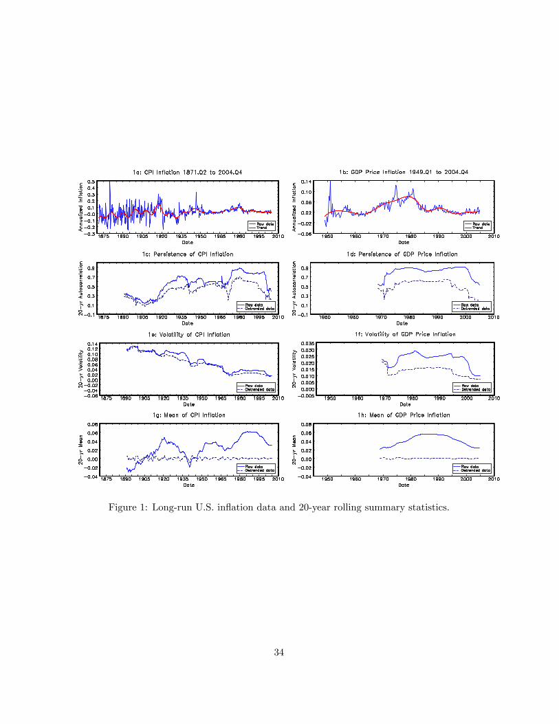
Figure 1: Long-run U.S. in�ation data and 20-year rolling summary statistics.

34

Figure 2: Determination of �� for consistent expectations equilibrium.

35

Figure 3: E¤ect of Kalman gain parameter on in�ation persistence and volatility.

36

Figure 4: Sampling variation in the autocorrelation of ��t a¤ects real-time learning paths.

37

Figure 5: Identifying the signal-to-noise ratio and the Kalman gain parameter from U.S. data.

38

Figure 6: Comparing survey-based U.S. expected in�ation to model-based values.

39

Figure 7: Properties of forecast errors when �t is generated using subjective forecast rule (9).

40

Figure 8: Simulated in�ation dynamics for three di¤erent forms of expectations.

41

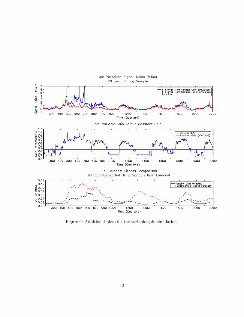
Figure 9: Additional plots for the variable-gain simulation.

42