time varying volatilities of output growth and inflation...
TRANSCRIPT

1
Preliminary and Incomplete Do Not Quote
Time Varying Volatilities of Output Growth and Inflation: A Multi-Country Investigation
John W. Keating♠ Victor J. Valcarcel
July 22, 2011
Abstract
Changes in volatility of output growth and inflation are documented for 8 countries with at least 140 years of uninterrupted source data. Time-varying parameter vector autoregressions are used to estimate standard deviations. We find that volatilities are typically lower after World War II than in the entire period preceding the war, with the primary exception being for the Classical Gold Standard period. Both volatilities rise quickly with World War I and its aftermath, stay relatively high until the end of World War II and drop rapidly until the mid to late-1960s. This Postwar Moderation provides the largest decline in volatilities for each country, or one of the very largest declines. Volatilities typically reach their lowest levels during or after the Great Moderation. For most countries, the financial crisis has eliminated the gains associated with the Great Moderation, and in many gains from the Postwar Moderation have been eroded. We also find that permanent shocks to output account for nearly all of the fluctuations in the volatility of output growth while shocks that have only a temporary effect on output account for most of the fluctuations in the volatility of inflation. JEL Classification: E30, E31, E65
Keywords: The Great Moderation; stochastic volatility; permanent-transitory decompositions;
Markov Chain Monte Carlo; structural vector autoregressions.
We thank Tim Cogley and Luca Gambetti for helpful correspondence and sharing Matlab code. This paper was presented July 1 at the 2011 Western Economic Association Meetings in San Diego. Thanks to participants in that session for constructive comments. The customary disclaimer applies. ♠ Department of Economics, The University of Kansas, 334 Snow Hall, Lawrence, KS 66045 E-mail: [email protected] Department of Economics, Texas Tech University, 257 Holden Hall, Lubbock, TX 79409 E-mail: [email protected]

2
1. Introduction
There is growing evidence that economic activity is not well-characterized by constant
volatility. Empirical research has found a substantial decline in the volatility of macroeconomic
aggregates beginning between the late-1970s to the mid-1980s.1 This period has been identified
as the Great Moderation, and a large literature has developed to explain this event. Many of
these empirical studies have focused on the United States.2 And the vast majority of
investigations focus solely on post-World War II experience. This paper examines evidence on
the volatilities of output growth and inflation using a set of 8 countries for which very long
uninterrupted time series are available. We take a multi-country approach to determine if there
is robust evidence on variation over time in volatilities. Our goal is to determine if any
important implications about the structure of the economy or about the role of policy emerge
from this study.
This research is motivated by a number of important questions. The initial question is:
How have volatilities behaved over this long span of time? Given the finding that both variables
exhibit trends and fluctuations in volatility, with particularly large fluctuations in inflation’s
volatility, we next ask: Do these patterns of variation share any similarities across countries? A
remarkable number of patterns are found to be robust across different economies. These robust
tendencies raise the question: Can observed movements in volatility be associated with changes
in policy or with non-policy events?
To address these questions, we use recently developed techniques for vector
autoregression (VAR) modeling that allow for time-varying parameters. Our specification
allows VAR coefficients to potentially change at each point in time and for possible stochastic
1 See Blanchard & Simon (2001); McConnell & Perez-Quiros (2002); Stock & Watson (2002); Davis &Khan (2008); and Nason & Smith (2008) among others. 2 With some notable exceptions. See Summers (2005) for an investigation of the G7 countries and Cecchetti et al (2006) who conclude that a great moderation in the mid 1980s can be found in the majority of OECD countries.
3
volatility in the errors.3 We use this model to estimate volatilities for real output growth and
inflation for countries that have uninterrupted annual source data spanning 140 years or more.
Our study is motivated in part by the common wisdom that the Great Moderation was
unprecedented. In contrast to that view, we present evidence of periods in which even greater
moderations have occurred. Following World War II, the volatilities of output growth and
inflation typically fell by as much as during the Great Moderation, and typically by even more.
This period has been labeled the Postwar Moderation.4 In many cases, much of the
improvement associated with the Great Moderation merely corrects the rise in volatility that
occurred during the 1970s. We also find that volatilities of inflation and output growth are
relatively low during the Classical Gold Standard period. Evidence of other moderations
provides a better understanding of the scale and the significance of the so-called Great
Moderation. We also find that volatilities are nearly always lower after the Postwar Moderation
than in the preceding period, excluding the Classical Gold Standard period.
An immediately relevant question is then addressed: Has the recent financial crisis cut
into stability gains achieved during the Great Moderation or the Postwar Moderation? In nearly
all countries, the gains from the Great Moderation have been completely eroded. In fact, in
many cases, the volatilities are now higher than the lowest levels reached during the Postwar
Moderation. This does not mean policymakers are incapable of bringing the economy back to
relative stability, but it does suggest that will take a long time for many countries to achieve.
It would be very interesting to determine the structural factors behind these robust
cross-country patterns in volatilities. One approach is to identify structural shocks from the
reduced-form and use these shocks to interpret the data. Clearly this road is subject to a host of
3 It seems particularly reasonable to allow shock variances to change when studying an economy over a long period of time. 4 Keating and Valcarcel (2011a)
4
well-known difficulties (outline them?…). And so there is no generally accepted framework for
performing investigations of this nature. Perhaps the most widely accepted identification
scheme in the literature comes from Blanchard and Quah (1989); though even this approach is
fraught with a host of potential concerns (list them? …). Blanchard and Quah decompose
output into permanent and transitory shocks, and if their identifying assumptions are valid
structural assumptions, the permanent shock to output is an aggregate supply (real) shock and
the transitory shock is an aggregate demand (nominal) shock.
In contrast to Blanchard and Quah (1989) and most of the literature that builds on their
work, we identify the permanent and transitory shocks using a time-varying VAR model. We
find that changes in volatility for output growth are primarily associated with the permanent
shocks to output while most changes in inflation volatility are associated with the temporary
shocks.
While most of the previous research has omitted data from earlier periods we are not the
first to examine changes in volatility from a historical perspective. For example, Romer (1999),
Nason and Smith (2008) and others (???) have also considered the historical evidence. An
important difference from these other papers is that we econometrically estimate when and
how volatilities change. Previous researchers assumed volatilities were constant over arbitrary
subsamples. Our approach is to let the data speak for itself by remaining agnostic about dates in
which standard errors may have changed. Another advantage of our model, relative to a more
traditional fixed-parameter approach, is that it allows us to determine if moderations take place
gradually or very rapidly.
The paper is organized as follows. Section 2 constructs the time-varying parameter
model, specifies the identification strategy, and describes the analysis of second moments.
Section 3 discusses data issues and sources. Section 4 describes our results for time-varying

5
volatilities of output growth and inflation. Section 5 examines the role of permanent and
transitory shocks to output in explaining movements in volatilities. We conclude by discussing
our main findings, examining the implications of those findings and outlining potentially
worthwhile avenues for future research.
2. The Time-Varying VAR and the Decomposition of Permanent and Transitory Shocks
We model the time series using a VAR that allows for time variation in the
autoregressive coefficients and shock covariance matrix. This framework does not require any a
priori assumptions about the timing, frequency, or size of possible changes in parameters. An
important advantage of using a time-varying parameter approach is that it allows us to estimate
a model that combines data from periods when an economy behaved quite differently. It used
to be common for economists to estimate fixed parameter models using sample periods that
excluded potentially extreme events such as World War I, The Great Depression and World
War II. Many believed that the economy operated in a fundamentally different way during
periods of global warfare or world-wide depression and, thus, the parameters would take on
different values. A time-varying parameter model allows us to include these unusual periods of
time in the estimation and to formally address the hypothesis that the parameters are different.
Our approach is similar to those of Cogley and Sargent (2001, 2005), Primiceri (2005),
and Galí and Gambetti (2009). Consider an l -th order VAR process
(L)x =t t te (2.1)
where xt is an n-vector of endogenous variables determined at time t, each jt in
1(L)=I ... lt t ltL L is a matrix of time-varying coefficients, and et is an n-vector of mean-

6
zero VAR innovations with the time-varying covariance matrix tR . The coefficients in (2.1)
evolve according to5
1t t tu (2.2)
where ut is Gaussian white noise with zero mean and constant covariance matrix Q,
independent of et at all leads and lags.6 The model reduces to a VAR with fixed coefficients and
stochastic volatility if 0tu for all t. For convenience we omit means from this exposition, but
in the estimation we allow the means to be time-varying following a process analogous to the
autoregressive parameters in (2.2). We use a variant of the Jaquier et al. (1994) stochastic
volatility framework that decomposes the covariance matrix of the reduced-form VAR as
follows:
Let ( )t t t t t tE e e R FH F¢ ¢º = where F is given by 2,1,
,1, , 1,
1 0 0
1
0
1
tt
n t n n t
fF
f f -
æ ö÷ç ÷ç ÷ç ÷ç ÷ç ÷= ç ÷÷ç ÷ç ÷ç ÷ç ÷ç ÷çè ø
and
1,
2,
,
0 0
0
0
0 0
t
tt
n t
h
hH
h
æ ö÷ç ÷ç ÷ç ÷ç ÷ç ÷= ç ÷÷ç ÷ç ÷ç ÷ç ÷ç ÷çè ø
The diagonal elements of tH are independent univariate stochastic processes that evolve
according to the following:
1ln ln 1,2,jt jt th h j nx-= + = (2.3)
where (0, )t iidx X . This random walk specification allows us to focus on permanent shifts in
the innovation variance —such as those that are emphasized on the U.S. economic stabilization
5 This is a parameterization of a more general law of motion 1 1
| , | ,t t t t t
p Q I f Q
for the posterior densities of the
states where tI is an indicator function that carries out the rejection sampling mechanism necessary to rule out explosive paths
of x. 6 According to Primiceri (2005), this assumption is not necessary but it allows for more efficient computations.
7
literature (Cogley and Sargent 2005)—while reducing the dimensionality of the estimation
procedure (Primiceri 2005.)7
We stack all the off-diagonal elements of 1tF- into a vector tg and, following Primiceri
(2005), we assume that this vector evolves according to the following drift-less random walk
1t t tg g z-= + (2.4)
where (0, )t iidz Y . All innovations are assumed to be jointly normally distributed, and our
bivariate application assumes the following covariance matrix of the system:
0 0 0
0 0 0var
0 0 0
0 0 0
t
t
t
t
I
u Q
e
xz
æ é ù ö é ù÷ç ê ú ê ú÷ç ÷ç ê ú ê ú÷ç ÷ê ú ê úç ÷ =ç ÷ê ú ê ú÷ç X÷ç ê ú ê ú÷ç ÷ç ê ú ê ú÷ç Y÷ç ê ú ê úè øë û ë û .
where each vector of shocks ( , , ,t t t tue x z ) consists of two elements.
te is a vector of uncorrelated
structural shocks with unit variance, Q ,X , and Y are positive definite 2x2 matrices, I is a 2x2
identity matrix and 0 is a 2x2 matrix of zeros. None of the off-diagonal zero restrictions are
required for estimation.8 However, allowing for an entirely unrestricted correlation structure
among the different sources of uncertainty would negate any structural interpretation of the
innovations.
Following Galí and Gambetti (2009), we assume that the innovations ( )te of the reduced–
form system (2.1) are a time-varying transformation of ( )et that satisfy ( )e e¢ = "t tE I t . Thus,
we have the following
t t te tj e= " (2.5)
7 This presents an alternative to ARCH models where the variances are generated by an unobserved components (UC) approach. 8 Primiceri (2005) outlines a minor modification to the estimation scheme to allow for non-zero off-diagonal blocks.
8
where tj is a nonsingular matrix that satisfies t t tRj j¢ = . Given this normalization
scheme, changes in the contributions of different structural shocks to the volatility in
innovations in the underlying variables of interest are captured by changes in tj .9 The
identification of shocks has nothing to do with the unconditional volatilities that will be the
major focus of the discussion that follows. These volatilities are derived directly from the
reduced form and do not depend on the identification of permanent and transitory effects on
the level of output. Conditional volatilities are the only ones that depend on these shocks.
Let the companion form of (2.1) be given by
1X = Xt t t tDe-Q + (2.6)
where 1 1X ( , ,..., )t t t tx x x , ( ,0,..., 0)D I , both of these matrices have the same
dimensions, and tQ is the companion-form matrix derived from the autoregressive coefficients
in (2.1). A standard local projection of (2.6) yields
2,2( ) , 0,1,2,t k kt
t
xs t k
e
+¶= Q " =
¢¶ (2.7)
where 2,2( )s · is the appropriate selector function.10 Application of the chain rule yields the
following impulse responses at an arbitrary k-th horizon
2,2( ) , 0,1,2,t k t k t kt t
t t t
x x es t k
ej
e e+ +¶ ¶ ¶
= = Q " =¢ ¢ ¢¶ ¶ ¶
(2.8)
Our model is based on ty , the logarithm of real output, and tp , the logarithm of the price
level, and both variables are first differenced: =t t tx y p . For the identification of shocks,
the effects on the levels of p and y are of interest. That requires the use of cumulative impulse
9 This model is general enough to allow for feedback between disturbances in drift and the covariance of the system even under more restricted scenarios than what we pose here. 10 Technically, the selector function is given by 2,2( )k k
t ts D D¢Q = Q which selects the upper left 2-by-2 matrix from the larger
matrix.
9
responses which are obtained as follows. First, we define 0
kk jt t
j=
Q = Qå . The level response of each
variable to each shock after k periods is the accumulated response of the differenced series from
period zero to period k. Then, following equation (2.8), the accumulated responses are given by
, 2,20
( )k
jt k t t
j
M s j=
º Qå . Finally, from the properties of the selector function, we obtain
, 2,2( )kt k t tM s j= Q . Furthermore, letting k ¥ allows us to define 2,2( )t t tM s j¥º Q as a time-
varying matrix of cumulative multipliers which measure the long-run effect of each shock on
output and the price level.
The underlying structural shocks, ( )P Tt t te e e ¢= , are identified by the assumption that a
transitory shock does not affect the output level in the long run. This implies that our matrix of
cumulative long-run multipliers is lower triangular. Thus, from the definition of tM
2,2 2,2( ) [ ( )]t t t t tM M s R s¥ ¥¢ ¢= Q Q .
(2.9)
tM is obtained as the Cholesky factor of the right-hand-side of (2.9). Given tM , we can solve for
tj as a function of the parameters in the VAR and obtain the structural impulse responses of
each shock occurring at time t: (Do we really need or want to have transposes on εin the
following equation or 2.7 or 2.8???)
1
2,2 2,2( ) ( ) , 0,1,2t k kt t t
t
xs s M t k
e
-+ ¥¶ é ù= Q Q " =ê úë û¢¶
With the exception of the long-run output response to a transitory output shock, every response
of each variable to each disturbance may evolve over time.
Note that tM is calculated in essentially the same way as Blanchard and Quah (1989),
except for two important differences: First, we allow for time variation in the coefficients and
10
the covariance matrix of residuals. And secondly, inflation is used as the second variable in the
model, in contrast to Blanchard and Quah (1989) who used the unemployment rate.
Each variable in our model has a time-varying moving average representation that is
driven by the two underlying “structural” disturbances, the permanent and transitory shocks to
output. Letting xit represent each variable, recursive substitution yields the following time
varying moving average representation:
, ,, ,
0 0
x [ ] [ ] ,P T
i P Tit t t k t k t k t k t t
k ki i
N N for i y pm e e¥ ¥
- -= =
= + + = D Då å (2.10)
(why do we need these N’s when we have Mt,k which has already been defined and seems to be
the same thing????) where , 2,2( )kt k t tN s jº Q applies the selector function, 2,2s , to the matrix of
autoregressive coefficients tQ from the companion form of the VAR, raised to the power k.
From (2.11) we determine how the time-varying unconditional variance of xit is decomposed
into the contribution from each shock:
, ,
2 2t 2,2 2,2
0 0
var (x ) [ ( ) ] [ ( ) ] i ,P Ti i
k kit t t t t t t
k k
s s for y pj j¥ ¥
= =
= Q + Q = D Då å (2.11)
It is important to stress that while this permanent-transitory shock decomposition serves as a
means of identifying orthogonal shocks that may be given structural interpretations, is has no
effect on the unconditional variances.
3. Data and Sources
11
We selected countries for which uninterrupted annual time series of inflation and real
output growth are available going well back into the 19th century. In almost all cases, these
series were computed on the basis of aggregate output measured in nominal and real terms.
The only exception is Canada in the 1870 to 1960 period for which variables are constructed
from nominal GDP and the GDP deflator. One advantage of a relatively long data sample is that
it permits examination of how volatilities evolved over extremely different economic
conditions. We allow for potentially different estimates in the nineteenth century, the periods of
world-wide warfare, the Great Depression and the post-World War II period, and don’t
constrain estimates to be constant within a period. The long series requirement does, however,
limit our study to 8 countries - the United States, the United Kingdom, Sweden, Italy, Finland,
Denmark, Canada and Australia. Most countries do not have reliable series of comparable
length. There are a number of other countries that do have data of similar quality and length,
but have breaks in the series, typically around a world war. Another advantage of using a long
sample period is that it facilitates a comparison between the results of this paper and those of
previous papers that draw from two different samples of historical US data.11,12
Table 1 describes in detail the data used in our analysis. In all cases, we needed to splice
output growth and inflation rates obtained from different sources. Details on the various
measures (GNP, GDP, Chain-Weighted or not), sources, splice dates, and base years for
calculating real output are found in Table 1. It is important to point out that despite various
differences in available data, our key results are very robust.
11 Keating and Valcarcel (2011a, 2011b) 12 We used the data from Romer (1989). It has been suggested by Romer (1986) and others that the volatility reduction in output growth during the 1940s could be due to measurement error. In a related paper, Romer (1989) constructs a new GNP series from relatively more accurate pre-1909 data on commodity output. She finds that the interwar period stands out as a time of "immoderation" flanked by periods of similar volatility in output growth. Balke and Gordon's (1989) method does not yield this result, however. Our results are quantitatively robust whether we employ the Balke-Gordon or Romer data sets. We find that since 1960 volatilities are virtually always smaller than they were in the pre-World War I period.12 Allowing for time-variation apparently can have a significant effect on how volatilities compare across time.
12
Splicing data that differ in terms of quality or method for computing real output would
cause major concern if we used a fixed parameter model. But splicing is less problematic in our
case because changes in data quality may be handled by changes in shock variances and/or
changes in VAR coefficients. Also, note that we experimented with alternative data and various
splice dates and obtained remarkably similar findings.13 (Vic, maybe we should do one more
experiment using longest span of Mitchell series – and/or possibly stopping in 1960 - for
splicing to US NIPA. And if possible we may think of alternative splicing dates for other
countries)
Each series is plotted in the Appendix. Henceforth, all references to output pertain to the
real measure of output unless stated otherwise.
4. Evidence on Time Varying Volatilities
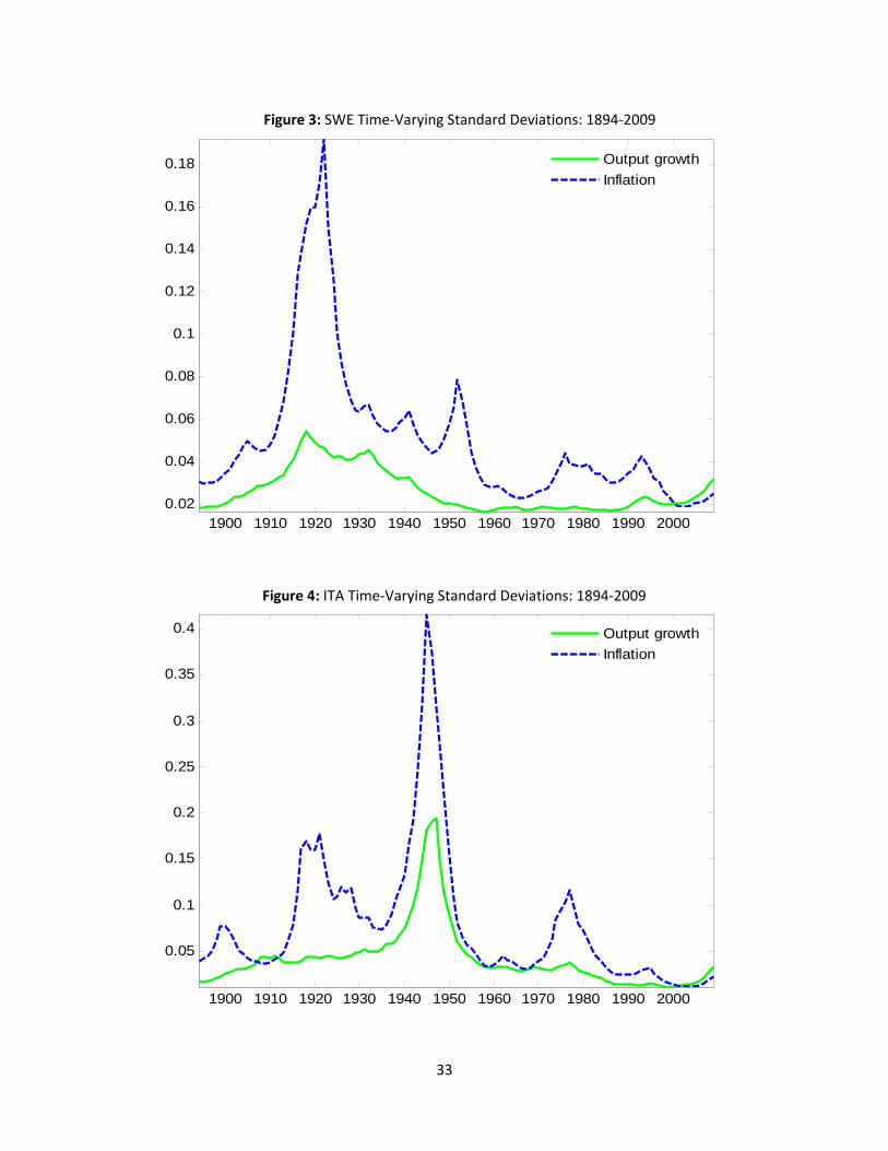
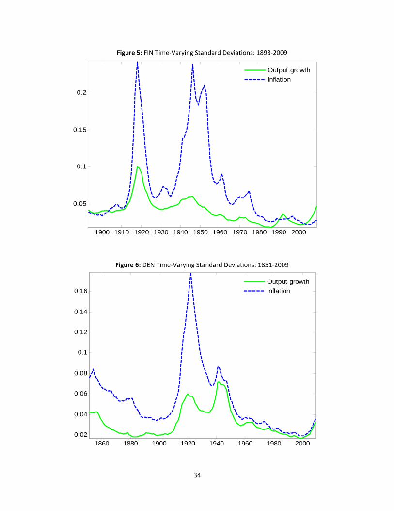
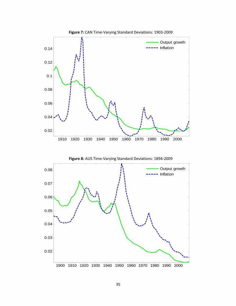
Figure 1 reports time‐varying standard deviations of output growth and inflation for the United
States. Figures 2 through 8 report standard deviations for the other 7 countries. Solid lines denote
volatilities of output growth while dashed lines denote inflation volatilities.
4.1 Output Growth Volatilities
Focusing initially on the United States, we find that the results here is qualitatively the same as
in Keating and Valcarcel (2011a,2011b), who estimated the model using different measures of pre‐1930
United States output data. Output volatility is relatively low before World War I. From the
beginning of World War I to shortly after the Korean War, output volatility is virtually always
13 Mitchell provides an alternative data source. And this made possible alternative dates for splicing and allowed for output to be measured in GDP or GNP. We also used Romer (1989) data from 1869 to 1929 in place of the series from Balke and Gordon. All findings in this paper are robust to these alternatives.
13
higher than at any other period in the sample. But starting shortly after World War II, output
volatility began to fall dramatically until the mid- to late-1960s. During this Postwar
Moderation, output’s standard deviation fell by roughly 60(???) percent. Volatility stabilized
for some time, and then in the early 1980s it began falling again reaching its minimum in the
mid-1990s. This most recent decline is known as the Great Moderation, but it pales in
comparison to the decline in output growth volatility during the Postwar Moderation. At the
end of the sample period, output growth volatility rises back to the level it had just before the
Great Moderation began.
Adding the other 7 countries to this discussion, we see that in all cases output growth volatility
declines rapidly shortly after World War II. This period yields the largest decline in volatility for 6 of the
countries in our study. (Calculate percentage declines from the peak to ????). For the other two
countries, Finland and Sweden, the largest decline in output volatility occurs after World War I.
However, the second largest reduction in output growth volatility for these countries starts shortly after
World War II.
Following this decline, output growth volatility tends to be lower than the preceding period. This
always holds for the United States, Australia and Canada and nearly always holds for the United
Kingdom. For Sweden, Italy and Finland, output volatilities in the post‐WWII period are smaller than the
pre‐World War II volatilities in the vast majority of cases.
The moderations in output volatility that follow World War II are impressive for two reasons.
One reason is that this period yields the most rapid, or nearly most rapid, reduction in volatility for each
country. Secondly, the volatilities achieved at the end of this moderation are typically not too far from
the lowest levels reached up to that point in the sample for each country.
14
While output growth volatility tends to be lower in the post‐World War II period, there are three
exceptions to tendency that are interesting in their own right. The first one is the Classical Gold Standard
period (1880‐1913) where output growth volatility is unusually low for Italy, Sweden and Denmark. In
fact, if we exclude the Classical Gold Standard period for each country, output growth volatility is
almost always lower following the rapid post‐World War II decline in output volatility than any
preceding time.14 In nearly all cases, output volatility fell even to a lower level during the Great
Moderation which followed the Postwar Moderation. However, there are also periods following the
Postwar Moderation when output volatility reached unusually high levels . One example of this occurred
in the 1970s. In fact, volatility of output growth for the United Kingdom exceeds the lowest levels found
in the pre‐World War II period. More generally, output growth volatility tends to rise somewhat in the
1970s for most of the countries.
Finland and Sweden provide another example of relatively high volatilities for output growth in
the postwar. Both countries saw sizable increases during the early‐1990s. This period of increased
volatility coincides with a local (Scandinavian) financial crisis that began ??? and focused most
intensively on these two countries and Norway.
Another interesting finding is that output growth volatilities are rising and relatively high at the
end of the sample for the United Kingdom, Sweden, Italy, Finland, and Denmark. In fact, volatility is
rising at the end of the sample for all countries except Australia. This suggests that Australia’s economy
has been less sensitive to the world financial crisis. Consistent with that view is that during the Great
Recession, Australia’s output fell less than the other countries in our analysis.
14 United States output growth volatility tends to rise during the Classical Gold Standard, using Mitchell (2003b). While the volatility associated with temporary shocks is relatively low during that period the volatility associated with permanent shocks is rising. This implies that if it weren’t for the rising volatility from permanent shocks, output volatility would have been lower during the Gold Standard. The rise in volatility of output growth for the United States during that period might be explained by the US being particularly well-suited to taking advantage of the innovations that came about during the Second Industrial Revolution. As we know, the US jumped ahead of the United Kingdom. One could expect that the innovations in the US contributed to both relatively rapid growth in output and relatively high variance from greater risk taking.
15
4.1 Inflation Volatilities
Figures 1 through 8 also report the volatility of inflation for each country. Looking first
at the US results we see that initially this volatility was low and falling. But it begins to rise
about the time of the Panic of 1907. Inflation volatility rises even faster during World War I
reaching the highest level in this sample a few years after the war has ended. Following a
smaller post-World War II spike, inflation volatility fell more in percentage terms than in any
other period. The steepest decline in inflation volatility occurs shortly after the 1951 Accord
between the Treasury and the Federal Reserve. The Fed’s obligation to peg the long-term
nominal bond rate was rescinded by this accord. By the mid-1960s it had fallen by roughly
76%???. Inflation volatility also experiences a Postwar Moderation. But, then inflation volatility
started to rise, slowly at first, and more rapidly as it spikes in the mid-1970s. Volatility stays
relatively high in the early 1980s, then falls reaching its lowest in-sample estimate in the 1990s.
Since then, it has increased a small amount and lies in the narrow range between the all-time
low from the 1990s and the low level it reached in the mid-1960s. At the end of the sample,
inflation volatility stays relatively low. In contrast, output growth volatility has risen roughly
back to the level it had just prior to the Great Moderation.
Adding the other 7 countries to the discussion yields a number of robust results, many
resembling the results for output growth volatility. For example, the lowest inflation volatility prior to
the end of World War II occurs during the Classical Gold Standard period. Inflation volatility falls rapidly
starting sometime after World War II, although in all cases, inflation volatility actually rises for a period
of time immediately following the war’s end. For Sweden, Finland, Canada and Australia this decline
doesn’t even begin until the 1950s, long after the war is over. But, by the 1960s inflation volatility
16
reaches its lowest level up to that point in the sample period for all countries except Finland which had
particularly low inflation volatility during the Classical Gold Standard. While inflation volatility shows a
strong tendency to be lower in the postwar period compared with the preceding period, there are
notable exceptions.
One exception is the 1970s during which inflation volatility for the United Kingdom, Sweden,
Finland, Italy, Australia and Canada often exceeds the low levels experienced during the Classical Gold
Standard period. This period contains world oil price shocks which caused spikes in inflation particularly
for oil importers.
Another important exception is that inflation volatility is rising at the end of the sample for
every country, except again Australia. This is particularly the case for the United Kingdom, Denmark and
Canada. Inflation volatility for the United States is also rising substantially at that time.
Inflation volatility rises to a local, if not global, maximum around the time of major wars. It
spikes for all countries after World War I and often reaches the highest level for a country.15 Inflation
volatility also tends to elevate during and after World War II, reaching maximum values at that time in
our samples for Italy and Finland.
It is interesting that these two velocities tend to be moving in opposite directions at the end of
World War II. In almost every case inflation volatility continues to rise for a number of years after the
war has ended while output growth volatility falls shortly after the war is over.
A large and rapid reduction almost always follows war‐related spikes in inflation volatility. Often
the largest decline occurs in the early 1920s. But this outcome is, in part, the result of the enormous rise
in inflation volatility that is associated with World War I and its aftermath. And while the decline in
15 The maximum US inflation volatility occurs shortly after World War I. However, using Mitchell’s (2003) data which provides a much longer time series, Keating and Valcarcel (2011a) find that peak inflation volatility occurs during the Civil War.

17
volatility is rapid, the level is not as low as the inflation volatility reached during Classical God Standard
period
5. Accounting for Changes in Volatility of Output Growth and Inflation
Equation (2.12) is used to calculate the standard errors conditioned on the permanent shocks or
the transitory shocks. By examining the contribution made by each shock we may provide a more
informative picture of the behavior of volatilities over time. Accounting for output growth and inflation
volatilities tends to yields much the same result across countries in our sample.
The Blanchard and Quah (1989) model may provide a structural means of assessing the sources
of changes in volatilities. If their assumptions characterize the actual structure implies that the
permanent output shocks are associated with aggregate supply and transitory shocks with aggregate
demand. Figure 9 illustrates how output growth volatility is decomposed into components associated
with these shocks to output at each point in time for each country. The contribution from temporary
shocks never exceeds and almost never comes close to the contribution made by permanent shocks.
The only times aggregate demand approaches aggregate supply’s contribution to output growth
volatility is a few cases in the period after World War I and a few from the mid‐1970s to the early 1980s.
The most striking feature in these graphs is how movements in output volatility are so closely mirrored
by changes in the contribution from permanent shocks. This result, interpreted in the context of
Blanchard and Quah’s model, suggests that fluctuations in the contribution from aggregate supply are
the primary factor explaining changes in output growth volatility.
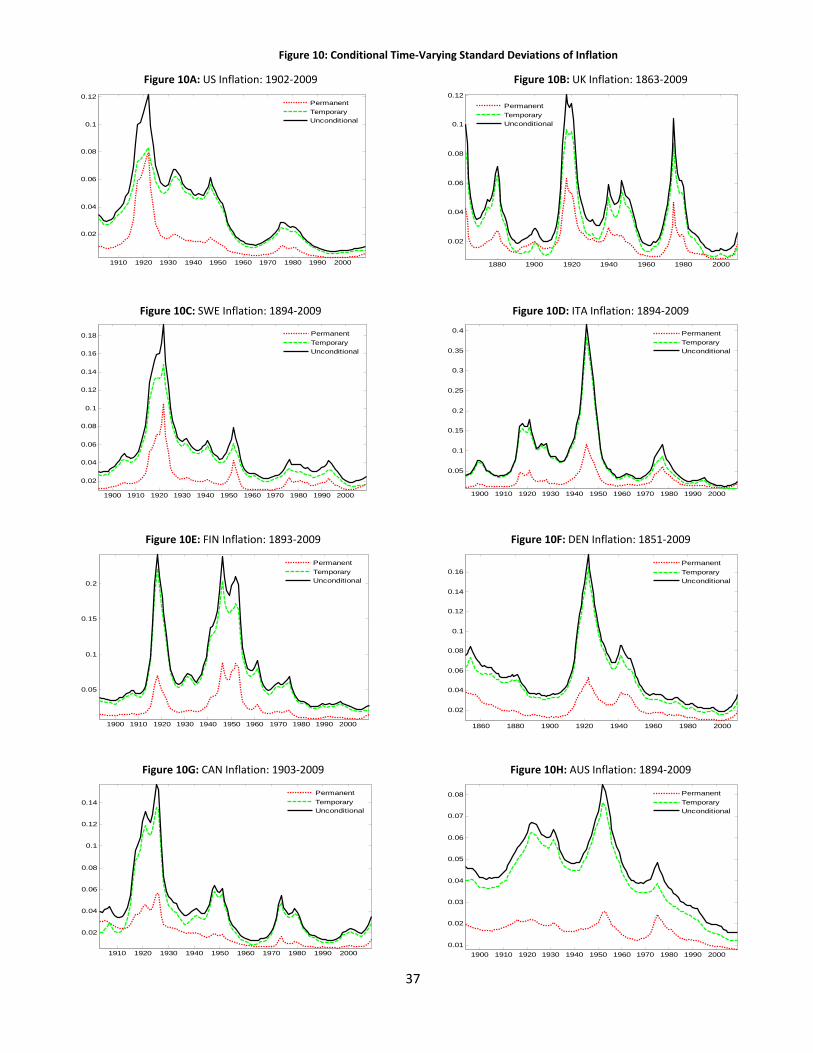
Figure 10 plots the volatility for inflation at each point in time for each country along with the
contribution from each of our two different shocks. For all countries we see that the fluctuations in
inflation volatility are usually mimicked by the contribution made by temporary shocks to output, and in
18
most countries it tracks quite closely. However, there are periods for some of the countries in which the
permanent shock accounts for nearly as much ‐ sometimes even more ‐ inflation volatility than the
temporary shocks. These exceptions occur during World Wars, the mid‐1970s to early‐1980s and the
latter part of the sample. The Blanchard and Quah model implies that aggregate demand is the major
force behind changes in inflation volatility, but there were some periods when aggregate supply was
also important. For example, inflation volatility has tended to be quite low during the latter part of the
sample. The model suggests that policymakers somehow lowered aggregate demand’s contribution to
inflation volatility, and that this change elevated the relative contribution of permanent shocks.
Blanchard and Quah’s (1989) model is able to give structural interpretations if the identifying
assumptions are consistent with the economic structure. However, the assumption that aggregate
supply shocks are the only type that may have a permanent effect on output is not universally accepted.
A number of different economic theories (list them?) exist for which aggregate demand shocks, along
with supply, may have permanent output effects. In that case, the effects of these shocks would not be
directly applicable to one type of structural disturbance – instead, the shocks in the model would end up
being some combination of the structural disturbances.16
6. Conclusions not well organized and incomplete at this time
We find that volatilities rise quickly with World War I and its aftermath, stay relatively
high until the end of World War II or afterwards, and drop rapidly until the mid to late-1960s.
Volatilities are typically lower after World War II than in the entire period preceding the war,
except primarily for the Classical Gold Standard period. This result suggests that a greater
16 But, Keating (2010) shows how one may still infer qualitative information about the underlying structure from impulse responses and variance decompositions from permanent and transitory shocks even if demand shocks may also permanently affect the level of output.
19
emphasis of policymakers on stabilization policy during this period has yielded some success.
Policy discussions and procedures implemented during the post-World War II period have
expressed considerable concern about stabilization. For example, passage of the Employment
Act of 1946 in the US occurs just before the volatilities of output growth and inflation began
rapid descents. That timing suggests the Federal government’s intent “to promote maximum
employment, production and purchasing power” (15 USC, §1021) led it to adopt policies that
played a major role in the Postwar Moderation.
The lowest volatilities in the mid to late-1960s are typically larger than the lows achieved
during the Great Moderation, though they are sometimes very close in magnitude. And during
the post-WWII moderation, the reduction in both volatilities is similar to or greater than the
Great Moderation (both in terms of the change in the level and the percentage change). In most
cases, the Postwar Moderation is more substantial than the Great Moderation.
Volatilities tend to rise in the 1970s, particularly for inflation. Both volatilities tend to
rise in the late 1960s or early 1970s. In part, these increases in volatilities help make the Great
Moderation look more impressive than it really was, particularly for the US, the UK, Italy and
Canada.
During the 1970s inflation volatility rises, usually reaching a postwar high and output growth
volatility often increases though to a lesser extent. Part of the Great Moderation consists of bringing
volatilities back down toward levels achieved during the Postwar Moderation, gains that were lost as a
result of the events of the 1970s. One possible explanation for the 1970s would be if the variance of
supply shocks increased. Another possibility could be that monetary policy was not functioning properly.
Specifically, central banks may not have obeyed the Taylor Principle. In most theoretical models such
20
behavior yields an indeterminate equilibrium solution. Indeterminacy would raise the level of
uncertainty in the economy and thus volatilities would likely increase
Our results are much in the spirit of Blanchard and Simon (2001) who, based on U.S. data from 1952 to ???, argue that there has been a "steady decline in output volatility interrupted in the 1970s and early 1980s, with a return to trend in the late 1980s and the 1990s." Our own estimates suggest that the postwar moderation is characterized by a steady decline taking place over the better part of a decade for inflation and even longer for output growth. Our estimates of stability gains associated with the Great Moderation are also more gradual than what much of the literature suggests and more in line with the process described by Blanchard and Simon.
The financial crisis threatens to eliminate gains associated with the Great Moderation, in
nearly all countries, and for a number of countries it puts the gains from the Postwar
Moderation in jeopardy.
Both volatilities rise at the end of the sample for every country except Australia.
In nearly all cases, volatilities rise to levels not seen since the 1980s and sometimes even earlier.
This evidence suggests the Great Moderation may well be over for most countries. Furthermore,
recent volatilities now exceed lows reached in the 1960s (during the post-WWII moderation) for
the UK, Sweden, Denmark, Finland and Canada. This evidence suggests that most of the
countries in our sample are in jeopardy of losing some of the gains made during the post-WWII
moderation
However, the longer sample also shows that the Great Moderation may be over for most of the countries in our study. … We show that output volatility has been rising over the last few years. This has been observed by others using different methods and has caused some to question whether the Great Moderation has ended (Clark 2009). This recent rise in output volatility has cut into the gains made during the Postwar Moderation for most of the countries.
21
We also find that permanent shocks to output account for nearly all of the fluctuations in
the volatility of output growth while shocks that have only a temporary effect on output
account for most of the fluctuations in the volatility of inflation. The structure that motivates
Blanchard and Quah’s (1989) model suggests that fluctuations in output growth volatility are
largely attributable to aggregate supply. Of course, one may doubt that interpretation given that
there are a number of different economic models for which aggregate demand may have a
permanent effect on output. But even if the model is not valid in a structural sense, it does
provide empirical regularities that can be used to judge the validity of theoretical structural
models. For example, whatever the model’s source of permanent movements in output, this
must be the primary source of fluctuation in the volatility of output growth for the model to be
consistent with the evidence.
Explanations for reduced volatility fall under three main categories - structural
changes,17 changes in the design or implementation of policy18 or a reduction in the underlying
heteroskedasticity of the exogenous shocks themselves.19 It is interesting that while we find
volatilities for output growth and inflation both declined during the Great Moderation and the
Postwar Moderation, changes in volatility for each variable are primarily driven by a different
type of structural disturbance. This finding seems at odds with the good luck hypothesis.
“Good luck” would require a coordinated decline in variances of the two different structural
17 Better inventory management, for example, has been proposed by McConnell and Perez-Quiros (2000) and Davis and Kahn (2008) as one structural explanation. A second perspective is that policymakers have developed better procedures for stabilization. Clarida et al. (2000), Taylor (1993) and others have suggested that monetary policy became more forward looking in the 1980s and, with foresighted policy, was therefore able to reduce fluctuations in output and inflation. Clarida et al. (2000), Taylor (1993) and others have suggested that monetary policy became more forward looking in the 1980s and, with foresighted policy, was therefore able to reduce fluctuations in output and inflation. 18 Clarida, Gali, and Gertler (2000) argue that monetary policy was a major factor in the Great Moderation, while Sims and Zha (2006) find that the change in shock variances is most important. Stock and Watson (2002) find evidence that monetary policy plays some role, but one that is fairly modest. 19 As one example, Justiniano and Primiceri (2008) point to reductions in the variance of investment shocks as an important factor in stabilization. This third option has been dubbed the “good luck” explanation, suggesting that the nature of the shocks has been intrinsically ameliorated since the 1980s.
22
shocks, but they are uncorrelated by construction. Also, the fact that these moderations coincide
with actual policy changes—that can, in the context of many economic models, help stabilize an
economy—argues against that hypothesis.
For the United Kingdom and Denmark, inflation volatility during the Classical Gold
Standard period falls below levels reached in the preceding period and for a long time
afterwards.20 For the other countries, the first volatility calculations begin in the Classical Gold
Standard period, and lower estimates are not typically achieved until after World War II.
Output growth volatility during this period is also typically declining or at a relatively low level
that will not be eclipsed until decades later, except for Canada.21 There are also dramatic
declines in postwar output growth and inflation volatilities during the Breton Woods exchange
rate regime. Therefore, two of the most substantial declines in inflation volatility occurred when
the US had a fixed exchange rate policy.
While fixed exchange rate systems are associated with the largest reductions in
volatility, our results show that standard errors of inflation and output growth have been at or
near historic lows for the last two decades, a time when exchange rates were permitted to float.
(Or did some have fixed exchange rates at some times?)
One implication of these findings is that a fixed Exchange Rate can be conducive to economic
stability. The Classical Gold Standard is typically associated with the lowest volatilities for inflation and
output growth in the pre‐WWII period. And the Postwar Moderation coincides with exchanges rates
20 And Keating and Valcarcel (2011a) find a similar result using United States data from Mitchell (2003b) which provides a longer sample that begins in the late-1700s. 21 It is interesting that during the Classical Gold Standard, the Second Industrial Revolution largely took place. It is also interesting that output volatility increased for the United States, in contrast to the behavior observed for most of the other economies in our study under a fixed exchange rate system. Increased output volatility seems a natural concomitant with an industrial revolution for a country that is benefiting greatly from the revolution. Creative destruction would have been on a greater scale than usual. This is what helped propel the United States, which benefitted as much as any other country during the Second Industrial Revolution, past the United Kingdom and into the position of dominant world power.

23
being governed by the Bretton Woods System. However, a fixed exchange rate system is not necessary
to maintain or achieve low volatilities. In nearly all cases, the lowest volatility is achieved after Bretton
Woods when exchange rates were subject to greater flexibility
The Classical Gold Standard periods seems to be a natural experiment that shows how fixed
exchange rates serve to stabilize fluctuations in output growth and inflation, an outcome predicted by
many different macroeconomic models and theories.
While both volatilities peak around the time of major wars, output growth volatility tends to
peak closer to the end of the war while inflation volatility tends to peak afterwards. The volatility of
output growth is accentuated by war as each combatant is trying to produce enough output to sustain
victory while at the same time trying to destroy the opponent’s productive capacity. These dynamics
may explain the wider swings in production as the war progresses.
The delayed decline of inflation volatility is also interesting and likely the result of many
different factors. After war is over, a government will gradually unwind the controls placed on prices,
wages, production and the allocation of goods and resources. As controls are gradually lifted prices are
prone to unusually large adjustments. Another factor is that wars produce large deficits that are
typically monetized to some extent. This monetary stimulus may combine with the release of market
controls to cause inflation to rise at an accelerated rate which would lead to greater volatility. But
inflation doesn’t rise forever. At some point the first two factors will usually lessen. The controls are
finally all released and in most cases the need to finance debt by the printing press is abated. However,
another factor is that economies tend to fall into recession following a war. In part this is a consequence
of an economy undergoing a costly adjustment of going from being a military economy back to normal
production. Recession puts downward pressure on inflation, and that may cause a rapid reversal of the
initial upward movement in inflation which could create even more volatility.
24
There are a number of important topics for future research. One is to determine why
moderations occur. How well can economic factors account for variation in volatilities? This is an old
question that seems to boil down to 3 possible explanations: Policy changes, structural changes or good
luck. Another is to obtain data from additional countries that would allow us to investigate whether or
not the Postwar Moderation is a feature of more economies or to determine if the Classical Gold
Standard had similar effects on other countries.
One of our interesting findings is the relatively large reduction in volatilities for output
growth and inflation during the Postwar Moderation. Why did each of these volatilities
undergo its most impressive reduction starting shortly after World War II? When trying to
account for the Great Moderation, economists have focused on two general sources: policy
reaction or structural change. The more substantial Postwar Moderation may also be a
consequence of these potential sources of moderation. 22
Policy changes that coincide with the beginning of the Postwar Moderation are clearly
evident. For example, the volatilities of output growth and inflation begin their most rapid
descents about the same time as passage of the Full Employment Act of 1946. This act states
“Congress hereby declares that it is the continuing policy and responsibility of the Federal
Government … to promote maximum employment, production and purchasing power.” (15
22 And failing to find support for either of these, good luck (i.e. an exogenous reduction in shock variances) is another possibility.
25
USC, §1021). The government’s concern for achieving these objectives may have caused it to
take actions that helped to stabilize fluctuations in output growth and inflation.23
Another policy change that occurred near the end of the war is the establishment of the
Bretton Woods system that fixed the exchange rates of other countries to the dollar and tied the
dollar to gold. The system was motivated by a belief that stable currencies would add stability
to both the real economy and prices. Some believed Bretton Woods would return economies to
the levels of stability not seen since the Classical Gold Standard, which describes the period
from 1880 to 1913. Our estimates provide some support for this idea. Volatilities for inflation
and output growth were smaller during the Classical Gold Standard than at any other time
before 1945, and frequently much smaller. And both volatilities fell dramatically at the time the
Bretton Woods system was implemented.24
The scale of government spending may also affect volatility. Measured in terms of
outlays as a share of output, government appears to be permanently larger after World War II
compared to the period before World War I. Over the business cycle, government spending is
less volatile than private spending. Hence, if government accounts for a larger share of the
economy, it is quite possible the aggregate economy will become more stable.25
23 Clarida, Gali, and Gertler (2000) argue that monetary policy was a major factor in the Great Moderation, while Sims and Zha (2006) find that the change in shock variances is most important. Stock and Watson (2002) find evidence that monetary policy plays some role, but one that is fairly modest. 24 While fixed exchange rate systems are associated with low and sometimes rapidly falling inflation volatility, our results indicate that fixed rates are not necessary for maintaining very low levels of volatility. The standard errors of both inflation and output growth have been at or near their historic lows over the last two decades, a time when the U.S. let its exchange rate float. 25 See Andrés, Doménech, and Fatás (2008) for a recent look at some of the evidence and a DSGE model that can account for some of that evidence.
26
The role of government programs known as automatic stabilizers has also expanded in
the postwar period. Automatic stabilizers respond endogenously to the state of the economy,
requiring no modification to policies already in place. They serve to passively moderate income
fluctuations. Income taxes are one example of an automatic stabilizer. Since World War II, taxes
as a share of income in the U.S. have been persistently higher than they were in the pre-World
War I period. Higher taxes can make after-tax income less volatile, and that would tend to make
consumer spending less volatile. Consequently, aggregate output should also be more stable.26
Income support from unemployment benefits and Medicaid reduce output fluctuations for
similar reasons. And both of these programs became increasingly important in the post-World
War II period. Thus a greater role of automatic stabilizers in the postwar period may have
contributed to the Postwar Moderation.
Alternatively, the Postwar Moderation may have resulted from structural change that is
unrelated to government policies. The Great Moderation, for example, has been attributed to
innovations in inventory management by a number of authors.27 Whether or not inventories are
an important contributor to the Postwar Moderation is an empirical question. And other
changes in private spending behavior might also be critical factors. For example, consumption
accounts for about 70% of GDP in 2009, and consumer services account for roughly 47% of
GDP. Both GDP shares have risen at times during the postwar period. Services have increased
in part as a result of increased spending on healthcare and financial services, for example. Since
total consumption is less volatile than the rest of output and consumer services less volatile than
total consumption, it is plausible that a rise in consumption—or its services component—as a
26 Of course, higher tax rates may also have adverse consequences for economic growth. 27 See, McConnell and Perez-Quirós, (2000) and Davis and Kahn, (2008) for examples.
27
share of GDP would make output less volatile. This mechanism may be an important factor,
even after controlling for the effects automatic stabilizers have on consumption. 28
The time variation in volatility is often associated with policy (fixed exchange rates, the postwar decision to put more emphasis on stabilizing business cycles, possible failure to follow the Taylor Principle) and non-policy events (WWI , WWII, 1970s supply shocks)
28 An interesting question is how much of a change in aggregate output volatility can be attributable to different spending components. While Blanchard and Simon (2001) made some progress on this issue, future research may develop new methods to better account for variation in volatility and share of spending for each spending component.
28
References Andrés, J.; Doménech, R.; Fatás, A. (2008) “The Stabilizing Role of Government Size” Journal of Economic Dynamics and Control 32: 571–593 Benati, L; Surico, P. (2009) “VAR Analysis and the Great Moderation” American Economic Review 99(4), 1636-1652 Balke, N.; Gordon, R. (1989) ”The Estimation of Prewar Gross National Product: Methodology and New Evidence” Journal of Political Economy 97(1):38-92. Bayoumi, T.; Eichengreen, B. (1994) ”Macroeconomic Adjustment under Bretton Woods and the Post-Bretton Woods Float: An Impulse Response Analysis” The Economic Journal 104: 813-827. Bayoumi, T.; Taylor, M.P. (1995) “Macroeconomic shocks, the ERM and Tri-Polarity” Review of Economics and Statistics 77: 321-331. Blanchard, O.J.; Quah, D. (1989) “The Dynamic Effects of Aggregate Demand and Supply Disturbances” The American Economic Review 79(4):655-673. Blanchard, O.J.; Simon, J. (2001) “The Long and Large Decline in U.S. Output Volatility” Brooking Papers on Economic Activity 2001-1:187-207. Bordo, M.D. (1993) “The Gold Standard, Bretton Woods and Other Monetary Regimes: A Historical Appraisal,” in M.T. Belongia ed. Dimensions of Monetary Policy: Essays in Honor of Anatol B. Balbach, Federal Reserve Bank of St. Louis, 123-191. Cecchetti, S., Flores-Lagunes, A., & Krause, S. (2006) “Assessing the sources of changes in the volatility of real growth. ” NBER Working Paper No. 11946. Clarida, R.; Galí, J.; Gertler, M. (2000) “Monetary Policy Rules and Macroeconomic Stability: Evidence and Some Theory” Quarterly Journal of Economics 115:147-180. Clark, T.E. (2009) “Is the Great Moderation Over?: An Empirical Analysis” Economic Review, Federal Reserve Bank of Kansas City (4):5-42. Cogley, T.; Sargent, T.J. (2001) “Evolving post World War II U.S. Inflation Dynamics” NBER Macroeconomics Annual 16:331-373. Cogley, T.; Sargent, T.J. (2005) “Drifts and Volatilities: Monetary Policies and Outcomes in the Post WWII U.S.” Review of Economic Dynamics 8:262-302. Cover, J.P. Enders, W., Hueng, C.J. (2006) “Using the Aggregate Demand-Aggregate Supply Model to Identify Structural Demand-Side and Supply-Side Shocks: Results Using a Bivariate VAR” Journal of Money, Credit, and Banking 38, April,777-790
29
Davis, S.J.; Kahn, J.A. (2008) “Interpreting the Great Moderation: Changes in the Volatility of Economic Activity at the Macro and Micro Levels” Journal of Economic Perspectives 22(4):155–180. Fernández-Villaverde, J.; Rubio-Ramírez, J.F.; Sargent, T.J.; Watson, M.W. (2007) “ABCs (and Ds) of Understanding VARs” American Economic Review 97(3):1021–1026. Galí, J.; Gambetti, L. (2009) “On the Sources of the Great Moderation” American Economic Journal: Macroeconomics 1(1):26-57. Gambetti, L. Pappa, E. Canova, F. (2008) “The Structural Dynamics of U.S. Output and Inflation: What Explains the Changes?” Journal of Money, Credit and Banking 40: 369-388 Jacquier, E.; Polson, N.G.; Rossi, P.E. (1994) “Bayesian Analysis of Stochastic Volatility Models” Journal of Business and Economic Statistics 12:371-389. Justiniano, A.; Primiceri, G. (2008) “The Time-Varying Volatility of Macroeconomic Fluctuations” American Economic Review 98(3):604-41. Karras, G. (1994) "Aggregate Demand and Supply Shocks in Europe: 1860-1987," The Journal of European Economic History 22:79-98. Keating, J.W. (2010) “Interpreting Permanent and Transitory Shocks to Output When Aggregate Demand May Not Be Neutral in the Long Run” University of Kansas Working Paper Keating, J.W.; Nye, J.V. (1998) “Permanent and Transitory Shocks in Real Output: Estimates from Nineteenth-Century and Postwar Economies” Journal of Money Credit and Banking 30(2): 231-251.
Keating, J.W.; Valcarcel, V. (2011a) “Greater Moderations” Texas Tech University Working Papers and University of Kansas Working Paper series.
Keating, J.W.; Valcarcel, V. (2011b) “The Time Varying Effects of Permanent and Transitory Shocks to Output” Texas Tech University Working Papers and University of Kansas Working Paper series Maddock, R.; McLean, I. (1987) The Australian Economy in the Long Run, Cambridge U.Press McConnell, M. M.; Perez-Quiros, G.P. (2000) “Output Fluctuations in the United States: What has changed since the Early 1980s? American Economic Review 90, 1464-1476. Mitchell, B.R. (2003a) International Historical Statistics: Europe, 1750-2000 5th ed. Houndmills, Basingstoke, Hampshire ; New York : Palgrave Macmillan. Mitchell, B.R. (2003b) International Historical Statistics: The Americas, 1750-2000 5th ed. Houndmills, Basingstoke, Hampshire ; New York : Palgrave Macmillan.
30
Nason, J.M.; Smith, G.W. (2008) "Great Moderation(s) and U.S. Interest Rates: Unconditional Evidence" The B.E. Journal of Macroeconomics 8(1) (Contributions), Article 30 Primiceri, G.E. (2005) “Time Varying Structural Vector Autoregressions and Monetary Policy” Review of Economic Studies 72(3), 821-852. Romer, C.D. (1986) “Is the Stabilization of the Postwar Economy a Figment of the Data” American Economic Review 76:314-334. Romer, C.D. (1989) “The Prewar Business Cycle Reconsidered: New Estimates of Gross National Product, 1869-1908” Journal of Political Economy 97:1-37. Romer, C.D. (1999) “Changes in Business Cycles: Evidence and Explanations” Journal of Economic Perspectives 13(2):23-44. Sims, C.; Zha, T. (2006) “Were There Regime Switches in Monetary Policy?” American Economic Review 96(1), 54-81. Stock, J.; Watson, M. (2002) ”Has the Business Cycle Changed and Why?” NBER Macroeconomics Annual (Cambridge, Mass.: MIT Press) 159-218. Summers, P. (2005) “What Caused the Great Moderation?: Some Cross Country Evidence” Economic Review, Federal Reserve Bank of Kansas City (3):5-32. Taylor, J. (1993) “Discretion versus Policy Rules in Practice” Carnegie-Rochester Conference Series on Public Policy 39:195-214. The Employment Act, Act of Feb. 20, 1946, ch. 33, section 2, 60 Stat. 23, 15 USC, §1021 Urquhart, M.C. (1988) "Canadian Economic Growth 1870-1980” Institute for Economic Research, Discussion Paper No.734, Queen's University World Bank’s World Development Indicator (WDI) Statistics collected through HAVER ANALYTICS 60 E 42nd St., Ste. 3310, New York, NY 10165-3310, United States (212)986-9300, (212)986-5857 fax, http://www.haver.com

31
TABLE 1: Data Sources
Current Output Real Output or Deflator
United States
GNP 1869-1929 (USD) Source: Romer (1989)
GNP 1929-2009 (USD)
Source: NIPA
GNP 1869-1929 (1982 USD) Source: Romer (1989)
GNP 1929-2009 (chain-wtd 2005 USD)
Source: NIPA
United Kingdom
GDP 1830-1960 (GBP) Source: Mitchell (2003a)
GDP 1960-2009 (GBP)
Source: WDI
GDP 1830-1912 (1900 GBP) GDP 1912-1948 (1938 GBP) GDP 1948-1960 (1958 GBP)
Source: Mitchell (2003a) GDP 1960-2009 (2000 GBP)
Source: WDI
Sweden
GDP 1861-1960 (SEK) Source: Mitchell (2003a)
GDP 1960-2009 (SEK)
Source: WDI
GDP 1861-1950 (1908 SEK) GDP 1950-1960 (1970 SEK)
Source: Mitchell (2003a) GDP 1960-2009 (chain-wtd 2000 SEK)
Source: WDI
Italy
GNP 1861-1960 (Lira) Source: Mitchell (2003a)
GDP 1960-2009 (Euro)
Source: WDI
GNP 1861-1951 (1938 Lira) GNP 1951-1960 (1963 Lira)
Source: Mitchell (2003a) GDP 1960-2009 (chain-wtd 2000 Euro)
Source: WDI
Finland
GDP 1860-1960 (Markaa) Source: Mitchell (2003a)
GDP 1960-2009 (Euro)
Source: WDI
GDP 1860-1960 (1985 Markaa) Source: Mitchell (2003a)
GDP 1960-2009 (2000 Euro)
Source: WDI
Denmark
GDP 1818-1960 (DKK) Source: Mitchell (2003a)
GDP 1960-2009 (DKK)
Source: WDI
GDP 1818-1960 (1929 DKK) Source: Mitchell (2003a)
GDP 1960-2009 (2000 DKK)
Source: WDI
Canada
GDP 1870-1960 (CAD) Source: Urquhart (1988)
GDP 1960-2009 (CAD)
Source: WDI
PGDP 1870-1960 (1981 GDP deflator) Source: Urquhart (1988)
GDP 1960-2009 (2000 CAD)
Source: WDI
Australia
GDP 1861-1965 (AUD) Source: Maddock &McLean (1987)
GDP 1965-2009 (AUD)
Source: WDI
GDP 1861-1965 (1911 AUD) Source: Maddock &McLean (1987)
GDP 1965-2009 (chain-wtd 2007 AUD)
Source: WDI Sources: See the paper for the complete references to historical sources.
WDI refers to World Development Indicator issue by the World Bank. NIPA refers to National Income and Product Accounts issued by the Bureau of Economic Analysis.

32
1910 1920 1930 1940 1950 1960 1970 1980 1990 2000
0.02
0.04
0.06
0.08
0.1
0.12
Figure 3: Time Varying Standard Deviations: 1902-2009
Output growth
Inflation
1880 1900 1920 1940 1960 1980 2000
0.02
0.03
0.04
0.05
0.06
0.07
0.08
0.09
0.1
0.11
0.12Figure 3: UK Time Varying Standard Deviations: 1863-2009
Output growth
Inflation
Figure 1: US Time‐Varying Standard Deviations: 1902‐2009
Figure 2: UK Time‐Varying Standard Deviations: 1863‐2009
33
1900 1910 1920 1930 1940 1950 1960 1970 1980 1990 20000.02
0.04
0.06
0.08
0.1
0.12
0.14
0.16
0.18
Figure 3: SWE Time Varying Standard Deviations: 1894-2009
Output growth
Inflation
1900 1910 1920 1930 1940 1950 1960 1970 1980 1990 2000
0.05
0.1
0.15
0.2
0.25
0.3
0.35
0.4
Figure 3: ITA Time Varying Standard Deviations: 1894-2009
Output growth
Inflation
Figure 3: SWE Time‐Varying Standard Deviations: 1894‐2009
Figure 4: ITA Time‐Varying Standard Deviations: 1894‐2009
34
1900 1910 1920 1930 1940 1950 1960 1970 1980 1990 2000
0.05
0.1
0.15
0.2
Figure 3: FIN Time Varying Standard Deviations: 1893-2009
Output growth
Inflation
1860 1880 1900 1920 1940 1960 1980 20000.02
0.04
0.06
0.08
0.1
0.12
0.14
0.16
Figure 3: DEN Time Varying Standard Deviations: 1851-2009
Output growth
Inflation
Figure 5: FIN Time‐Varying Standard Deviations: 1893‐2009
Figure 6: DEN Time‐Varying Standard Deviations: 1851‐2009
35
1910 1920 1930 1940 1950 1960 1970 1980 1990 2000
0.02
0.04
0.06
0.08
0.1
0.12
0.14
Figure 3: CAN Time Varying Standard Deviations: 1903-2009
Output growth
Inflation
1900 1910 1920 1930 1940 1950 1960 1970 1980 1990 2000
0.02
0.03
0.04
0.05
0.06
0.07
0.08
Figure 3: AUS Time Varying Standard Deviations: 1894-2009
Output growth
Inflation
Figure 7: CAN Time‐Varying Standard Deviations: 1903‐2009
Figure 8: AUS Time‐Varying Standard Deviations: 1894‐2009

36
1910 1920 1930 1940 1950 1960 1970 1980 1990 2000
0.01
0.02
0.03
0.04
0.05
0.06
0.07
0.08
Figure 5: Conditional Standard Deviations for U.S. Real GNP growth: 1902-2009
Permanent
TemporaryUnconditional
1880 1900 1920 1940 1960 1980 2000
0.01
0.02
0.03
0.04
0.05
0.06
Figure 5: Conditional Standard Deviations for UK Real GDP growth: 1863-2009
Permanent
TemporaryUnconditional
1900 1910 1920 1930 1940 1950 1960 1970 1980 1990 20000.005
0.01
0.015
0.02
0.025
0.03
0.035
0.04
0.045
0.05
Figure 5: Conditional Standard Deviations for SWE Real GDP growth: 1894-2009
Permanent
TemporaryUnconditional
1900 1910 1920 1930 1940 1950 1960 1970 1980 1990 2000
0.02
0.04
0.06
0.08
0.1
0.12
0.14
0.16
0.18
Figure 5: Conditional Standard Deviations for ITA Real GDP growth: 1894-2009
Permanent
TemporaryUnconditional
1900 1910 1920 1930 1940 1950 1960 1970 1980 1990 2000
0.01
0.02
0.03
0.04
0.05
0.06
0.07
0.08
0.09
0.1Figure 5: Conditional Standard Deviations for FIN Real GDP growth: 1893-2009
Permanent
TemporaryUnconditional
1860 1880 1900 1920 1940 1960 1980 2000
0.01
0.02
0.03
0.04
0.05
0.06
0.07
Figure 5: Conditional Standard Deviations for DEN Real GDP growth: 1851-2009
Permanent
TemporaryUnconditional
1910 1920 1930 1940 1950 1960 1970 1980 1990 2000
0.01
0.02
0.03
0.04
0.05
0.06
0.07
0.08
0.09
0.1
0.11
Figure 5: Conditional Standard Deviations for CAN Real GDP growth: 1903-2009
Permanent
TemporaryUnconditional
1900 1910 1920 1930 1940 1950 1960 1970 1980 1990 2000
0.01
0.02
0.03
0.04
0.05
0.06
0.07
Figure 5: Conditional Standard Deviations for AUS Real GDP growth: 1894-2009
Permanent
TemporaryUnconditional
Figure 9: Conditional Time‐Varying Standard Deviations of Output Growth
Figure 9A: US Real GNP Growth: 1902‐2009 Figure 9B: UK Real GDP Growth: 1863‐2009
Figure 9C: SWE Real GDP Growth: 1894‐2009 Figure 9D: ITA Real GNP Growth: 1894‐2009
Figure 9E: FIN Real GDP Growth: 1893‐2009 Figure 9F: DEN Real GDP Growth: 1851‐2009
Figure 9G: CAN Real GDP Growth: 1903‐2009 Figure 9H: AUS Real GDP Growth: 1894‐2009
37
1910 1920 1930 1940 1950 1960 1970 1980 1990 2000
0.02
0.04
0.06
0.08
0.1
0.12
Figure 6: Conditional Standard Deviations for U.S. Inflation: 1902-2009
Permanent
TemporaryUnconditional
1880 1900 1920 1940 1960 1980 2000
0.02
0.04
0.06
0.08
0.1
0.12Figure 6: Conditional Standard Deviations for UK Inflation: 1863-2009
Permanent
TemporaryUnconditional
1900 1910 1920 1930 1940 1950 1960 1970 1980 1990 2000
0.02
0.04
0.06
0.08
0.1
0.12
0.14
0.16
0.18
Figure 6: Conditional Standard Deviations for SWE Inflation: 1894-2009
Permanent
TemporaryUnconditional
1900 1910 1920 1930 1940 1950 1960 1970 1980 1990 2000
0.05
0.1
0.15
0.2
0.25
0.3
0.35
0.4
Figure 6: Conditional Standard Deviations for ITA Inflation: 1894-2009
Permanent
TemporaryUnconditional
1900 1910 1920 1930 1940 1950 1960 1970 1980 1990 2000
0.05
0.1
0.15
0.2
Figure 6: Conditional Standard Deviations for FIN Inflation: 1893-2009
Permanent
TemporaryUnconditional
1860 1880 1900 1920 1940 1960 1980 2000
0.02
0.04
0.06
0.08
0.1
0.12
0.14
0.16
Figure 6: Conditional Standard Deviations for DEN Inflation: 1851-2009
Permanent
TemporaryUnconditional
1910 1920 1930 1940 1950 1960 1970 1980 1990 2000
0.02
0.04
0.06
0.08
0.1
0.12
0.14
Figure 6: Conditional Standard Deviations for CAN Inflation: 1903-2009
Permanent
TemporaryUnconditional
1900 1910 1920 1930 1940 1950 1960 1970 1980 1990 2000
0.01
0.02
0.03
0.04
0.05
0.06
0.07
0.08
Figure 6: Conditional Standard Deviations for AUS Inflation: 1894-2009
Permanent
TemporaryUnconditional
Figure 10A: US Inflation: 1902‐2009
Figure 10: Conditional Time‐Varying Standard Deviations of Inflation
Figure 10B: UK Inflation: 1863‐2009
Figure 10C: SWE Inflation: 1894‐2009 Figure 10D: ITA Inflation: 1894‐2009
Figure 10E: FIN Inflation: 1893‐2009 Figure 10F: DEN Inflation: 1851‐2009
Figure 10G: CAN Inflation: 1903‐2009 Figure 10H: AUS Inflation: 1894‐2009

38
1880 1900 1920 1940 1960 1980 2000
-0.1
0
0.1
U.S. Real GNP Growth: 1871-2009
1880 1900 1920 1940 1960 1980 2000
-0.1
0
0.1
0.2U.S. Inflation: 1871-2009
1840 1860 1880 1900 1920 1940 1960 1980 2000
-0.1
0
0.1
Figure 1: UK Log Real GDP growth: 1831-2009
1840 1860 1880 1900 1920 1940 1960 1980 2000
-0.1
0
0.1
0.2
Figure 2: UK Inflation rate: 1831-2009
1880 1900 1920 1940 1960 1980 2000-0.1
0
0.1
Figure 1: SWE Log Real GDP growth: 1862-2009
1880 1900 1920 1940 1960 1980 2000
-0.2
0
0.2
Figure 2: SWE Inflation rate: 1862-2009
1880 1900 1920 1940 1960 1980 2000
-0.2
0
0.2
0.4
Figure 1: ITA Real GDP growth: 1862-2009
1880 1900 1920 1940 1960 1980 2000
0
0.5
1
Figure 2: ITA Inflation rate: 1862-2009
Figure A1: US Real GNP Growth: 1871‐2009
Figure A2: US Inflation Rate: 1871‐2009
Figure A3: UK Real GDP Growth: 1831‐2009
Figure A4: UK Inflation Rate: 1831‐2009
Figure A5: SWE Real GDP Growth: 1862‐2009
Figure A6: SWE Inflation Rate: 1862‐2009
Figure A7: ITA Real GNP Growth: 1862‐2009
Figure A8: ITA Inflation Rate: 1862‐2009
Appendix : Real Output Growth Rate and Inflation Rate for Eight Countries

39
1880 1900 1920 1940 1960 1980 2000
-0.1
0
0.1
0.2Figure 1: FIN Log Real GDP growth: 1861-2009
1880 1900 1920 1940 1960 1980 2000
0
0.2
0.4
0.6
Figure 2: FIN Inflation rate: 1861-2009
1820 1840 1860 1880 1900 1920 1940 1960 1980 2000
-0.1
0
0.1
Figure 1: DEN Real GDP growth: 1819-2009
1820 1840 1860 1880 1900 1920 1940 1960 1980 2000-0.2
0
0.2
Figure 2: DEN Inflation rate: 1819-2009
1880 1900 1920 1940 1960 1980 2000-0.1
0
0.1
0.2
0.3
Figure 1: CAN Real GDP growth: 1871-2009
1880 1900 1920 1940 1960 1980 2000
-0.1
0
0.1
0.2
Figure 2: CAN Inflation rate: 1871-2009
1880 1900 1920 1940 1960 1980 2000
-0.1
0
0.1
Figure 1: AUS Real GDP growth: 1862-2009
1880 1900 1920 1940 1960 1980 2000-0.1
0
0.1
0.2
Figure 2: AUS Inflation rate: 1862-2009
Figure A9: FIN Real GDP Growth: 1861‐2009
Figure A10: FIN Inflation Rate: 1861‐2009
Figure A11: DEN Real GDP Growth: 1819‐2009
Figure A12: DEN Inflation Rate: 1819‐2009
Figure A14: CAN Inflation Rate: 1871‐2009 Figure A16: AUS Inflation Rate: 1862‐2009
Figure A13: CAN Real GDP Growth: 1871‐2009 Figure A15: AUS Real GDP Growth: 1862‐2009