Timing Pulse Measurement and Detector

Calibration for the OsteoQuant®

Advisor: Dr. Thomas N. Hangartner

By: Binu Enchakalody1

The OsteoQuant®

• pQCT scanner which can provide precise density assessment of the

trabecular and cortical regions of bone.

• Currently being upgraded to a x-ray tube source and a CZT

semiconductor detector.

2Ref: http://www.wright.edu/academics/bmil/bmil1.htm

1. Implement a system capable of registering the motor- and

detector timing-pulses of the Osteoquant® using a common time-

base in microsecond resolution.

2a. Correct the photon-count loss due to dead time to an error level of

less than 0.5% of the maximum expected photon counts.

2b. Correct the non-linearity of the projection values due to beam

hardening to an error level of less than 1% of the expected

maximum projection value.

Objective

3

Timing-Pulse Measurement

for the OsteoQuant®

4

Need for Timing-Pulse Measurement

• Data collected is only useful if there is synchronization between the

motor- and detector-timing pulses.

• The motor- and detector timing-pulses have to be well synchronized to

assure correlation between the data collected and the measurement

interval.

Aim

Each detector frame should be accurately related to a motor position.

Solution

Measure time stamps using a common time base to relate a motor

position to a detector frame.

5

Sample Detector Timing-Pulse

Sample Motor Timing-Pulse

Common Time-Base (1/1000 resolution)

0 3 6 9 12 ms

0 2 4 6 8 10 12 ms

1

µs

3000 6000 8000 10000 12000 9000 0 2000 4000 µs

Timing-Pulse Measurement: Analyzing the problem

6

• Requires counters working at clock frequencies of 1 MHz or above.

• High data transfer speed

• Fast event notification

Solution

• The USB-4301 is a low-power USB-2.0-compliant, 16-bit, 5

channel, up-down binary counter, capable of operating at frequencies

as high as 5 MHz can be used in event counting and pulse generating

applications.

Timing-Pulse Measurement: Requirement

7

Setup

• Motor- and detector-timing pulses are assigned to separate modules

• Modules are daisy chained to form 32-bit counters

• Terminal count is achieved in ~72 minutes

8

External Circuit Components

Synchronization Circuit

9

External Circuit Components

10

Timing Diagram

11

Flow chart

External Circuitry

• Pulse Shaping Circuit

• Start Pulse

• Synchronization Circuit

• Interrupt Mask

• Combined Circuit

Counter Programming

• Initialization

• Configuration

• Counter Save

• Time Stamp

12

Error Range of Measured Time Periods

• Interrupt signal of 2.22 ± 0.003 ms

• Relative error : 0.13%

13

Sample Spreadsheet

14

Detector Calibration for the

OsteoQuant®

15

Detector Calibration: Dead Time

Dead Time

• An event occurs at the detector is converted into an electrical signal

depending on the intensity and duration of the event.

• The time required to collect this charge depends on certain

characteristics (mobility, distance to collection electrodes, etc.) of the

detector itself and on the subsequent electronics.

• Due to the random nature governed by Poisson statistics, there is

always a probability that the detector misses a true event that follows a

recorded event.

• The missed true events are called dead-time losses

16

Need for Dead-Time Correction

The measured non-linear and the expected

linear photon counts for varying tube currents

of one detector element from a sample data set

Operating Parameters:

Tube Voltage : 45 kVp

Tube Current: 0 – 1 mA

Photon accumulation time : 50 ms

Aim:

Correct the photon-count loss

due an error level of less than

0.5% of the maximum

expected photon counts

(0.5% of 72,000) ± 350

counts.

The photon counts-vs.-tube

current response plot is

mathematically modeled and

then linearized.

CountsSlope

Current

17

Detector Calibration: Beam Hardening

Beam Hardening

• X-ray beams used in CT are usually polychromatic

• When the photon beam passes through material, it tends to

preferentially loose its lower energy photons, hardening the beam in the

process.

• Lower-energy x-rays are more prone to attenuation, and the average

energy of a polychromatic beam varies with increasing thickness of the

material, thereby making the beam harder.

18

Beam Hardening

Aim:

Correct the non-linearity of the

projection values due to beam

hardening to an error level of

less than 1% of the expected

maximum projection value (1%

of 5 projection value units) ±

0.05.

The projections-vs.-thickness

plot is mathematically modeled

and then linearized. The measured non-linear and

expected linear projection values for

varying absorber thicknesses.

Operating Parameters:

Tube Voltage : 45 kVp

Tube Current: 1 mA

Photon accumulation time : 50 ms

Pr ojectionSlope

Thickness

19

Experimental Setup

• Source : The tube can operate at a maximum anode voltage of 50 kVp

and a maximum anode current of 1 mA, at a maximum operating

temperature of 55oC.

• Detector : The detector is a CZT semi-conductor cuboid of 64 pixilated

elements composed of 50% tellurium, 5% zinc and 45% cadmium.

• Slabs : Slabs are used in the beam hardening experiment as a substitute

for the bone and soft-tissue in human-body (aluminum and Plexiglas). A

total on 19 pairs of these slabs were used.

• Data was collected on 22 dates over a span of nine months.

20

Dead-Time Correction: Steps

1. Modeling using the fourth-degree polynomial function

2. Linearization of the model

3. Drift and stability analysis of the correctioni. Same-date Correction

ii. Different-date Correction

21

Dead-Time Correction: Modeling and linearization

For dead-time correction

22

Stability of the Dead-Time Correction

• Fit-coefficient vectors were collected

• Corrections applied to the data collected at the same date (same-date

corrections) and a different-date (different-date corrections).

• The stability was analyzed by comparing the residuals

• The corrections were declared stable if their residuals < 350.

• The least expected residuals are those from the same-date corrections

23

Beam-Hardening Correction: Steps

1. Fifth-Degree Polynomial Modeli. Modeling using the polynomial function for 10- and 19-plate data sets

ii. Linearizing the mathematical model

iii. Corrections applied on the 10- and 19-plate data sets

2. Bimodal-Energy Modeli. Modeling using the bimodal-energy model for 10- and 19-plate data sets

ii. Linearizing the mathematical model

iii. Corrections applied on the10- and 19-plate data sets

3. Compare the stability analysis between both models

24

Beam-Hardening Correction

i : 1, 2, 3, ... 19 for the number of slab pairs used

I0 : counts collected with no object in the beam path

Ii : counts collected with i number of slab pairs

µeff : linear attenuation coefficient for Al and Pl

di : thickness of i number of slab pairs

The projection values are generally

linearized to a linear line.

According to Beer’s Law, the projection values of the x-ray beam passing

through an object are linearly proportional to μ(E).

25

Linearization Using the Polynomial Model

• Based on the projection value-vs.-slab thickness plots, it was decided that

an 5th-degree polynomial fit can model these data.

• Each detector element’s data was fitted using a second to a sixth-degree

polynomial function.

26

Bimodal-Energy Model

• The bimodal energy model* suggests that the attenuation is a function

of predominantly two energies, a dominant energy (E2) and a lower

energy (E1).

• The projection values can be modeled using μ1, μ2 and α.

• μ2 is the slope by E2 for large thicknesses

• μ1 is the slope by E1 for smaller thicknesses.

• To solve for the unknowns, the non-linear least squares method is

used.

• The equation system was iteratively solved using a Matlab script by

assuming initial values for the unknown fitting parameters.Ref: de Casteele, E. V., Dyck, D. V., Sijbers, J., and Raman, E. 2002. An energy-based beam hardening model

in tomography. Phys Med Biol 47, 23–30.27

Bimodal-Energy Model

Linear attenuation coefficient (μ(E)) vs. energy for the

Al/Pl slabs.

• The slab pairs were treated as a

homogenous material by calculating

the thickness ratio for a slab pair.

• Energies E2 and E1 are not

predetermined.

• Estimate of the expected lower and

upper bound for μ1 and μ2.

• E2 proved to be greater than E1

28

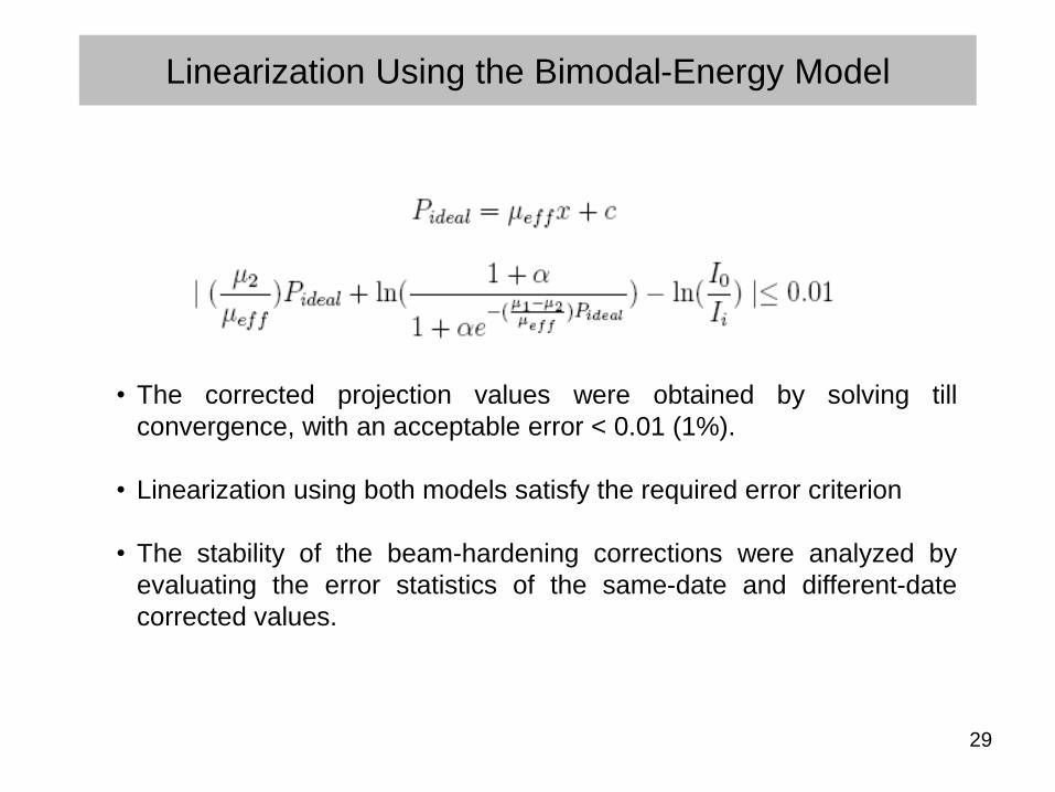
Linearization Using the Bimodal-Energy Model

• The corrected projection values were obtained by solving till

convergence, with an acceptable error < 0.01 (1%).

• Linearization using both models satisfy the required error criterion

• The stability of the beam-hardening corrections were analyzed by

evaluating the error statistics of the same-date and different-date

corrected values.

29

Secondary Correction

• Primary correction every day is a tedious process.

• Apply primary corrections from one particular date to the data sets

collected from other dates and following this with a secondary correction

(3rd degree polynomial) based only on a few plates (0, 6, 14, 19 or

0, 3, 7, 9) measured on the specific date.

Without Secondary Correction With Secondary Correction 30

Stability analysis for beam-hardening corrections

• Same-date and different-date corrections.– Same-date primary

– Different-date primary

– Different-date-primary followed by secondary

• Data collected on 22 dates, during nine months.

• 134 coefficient matrices for the 10-plate data sets.

• 5 coefficient matrices for the 19-plate data sets.

• Stability for the correction method is assumed if the residuals of the

same-date and different-date corrections are less than 0.05.

31

Results: Dead-Time Correction

Linearization using the fourth-degree model for a data set. Histogram of the individual residuals using

a fourth-degree polynomial correction for a data set

32

Same-Date Corrections: 10 plate data-set

33Corrected projection values and their histograms for the polynomial and

the bimodal-energy model

Different-date corrections: 10 plate data-set

Corrected projection values and their histograms for the polynomial and the

bimodal-energy model

34

Different-date primary followed by secondary correction:

10 plate data-set

35Corrected projection values and their histograms for the polynomial and

the bimodal-energy model

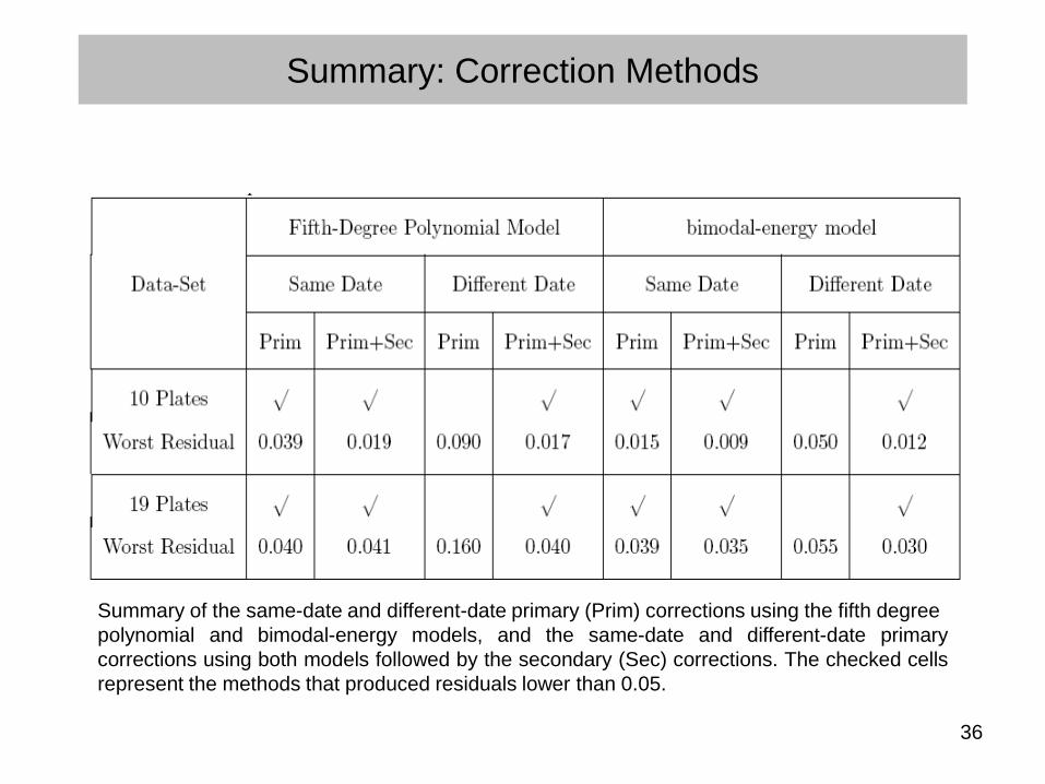
Summary: Correction Methods

Summary of the same-date and different-date primary (Prim) corrections using the fifth degree

polynomial and bimodal-energy models, and the same-date and different-date primary

corrections using both models followed by the secondary (Sec) corrections. The checked cells

represent the methods that produced residuals lower than 0.05.

36

Detector Calibration: Summary

• The same-date dead-time corrections were all within the expected

residual value.

• The data collection required for the dead-time corrections can be

automated.

• Same-date primary corrections consistently produced corrected projection

values that were well within the expected residual of 0.05.

• Most of the residuals for the different-date bimodal corrections were

below 0.05, whereas the residual values for the different-date polynomial

corrections were above 0.05.

Future Work

• Using the non-paralyzable dead-time model.

• Beam hardening corrections should be studied with different tube

voltages.

• Stability of the corrections over a shorter time period can be studied

37