tire contact patch characterization through finite …...abstract tire contact patch...
TRANSCRIPT

Tire Contact Patch Characterization through Finite Element Modeling and
Experimental Testing
Thomas Mathews Vayalat
Thesis submitted to the faculty of the Virginia Polytechnic Institute and State
University in partial fulfillment of the requirements for the degree of
Master of Science
In
Mechanical Engineering
Saied Taheri, Chair
Corina Sandu
Robert L. West
September 28th, 2016
Blacksburg, VA
Keywords: Tire, finite element modeling, footprint phenomena, contact patch,
steady state rolling, Fujifilm Prescale
Copyright © 2016, Thomas Mathews Vayalat

ABSTRACT
Tire Contact Patch Characterization through Finite Element Modeling and
Experimental Testing
Thomas Mathews Vayalat
The objective of this research is to provide an in-depth analysis of the contact patch behavior of a
specific passenger car tire. A Michelin P205/60R15 tire was used for this study. Understanding
the way the tire interacts with the road at various loads, inflation pressures and driving conditions
is essential to optimizing tire and vehicle performance. The footprint shape and stress
distribution pattern are very important factors that go into assessing the tire’s rate of wear, the
vehicle’s fuel economy and has a major effect on the vehicle stability and control, especially
under severe maneuvers.
In order to study the contact patch phenomena and analyze these stresses more closely, a finite
element (FE) tire model which includes detailed tread pattern geometry has been developed,
using a novel reverse engineering process. In order to validate this model, an experimental
process has been developed to obtain the footprint shape and contact pressure distribution. The
differences between the experimental and the simulation results are discussed and compared. The
validated finite element model is then used for predicting the 3D stress distribution fields at the
contact patch. The predictive capabilities of the finite element tire model are also explored in
order to predict the handling characteristics of the test tire under different maneuvers such as
pure cornering and pure braking.
GENERAL AUDIENCE ABSTRACT
Tire Contact Patch Characterization through Finite Element Modeling and
Experimental Testing
Thomas Mathews Vayalat
The objective of this research is to study how the tire interacts with the road and how this
“interaction” affects vehicle and tire performance. When the tire is in contact with the ground,
the region of the tire that is in contact with the surface is referred to as the “tire contact patch” or
the “tire footprint”. A Michelin tire was used in order to study this “footprint phenomena”. The
effects of weight, tire pressure and different driving conditions (such as braking and cornering)
have a very significant impact on the footprint phenomena. The footprint shape, size and
pressure distribution pattern are very important factors that go into assessing the tire’s rate of
wear, the vehicle’s fuel economy and has a major effect on the vehicle stability, especially under
severe maneuvers.
As conducting large scale experiments to study this phenomenon is expensive and difficult,
simulation methods (such as the finite element method) are used to create tire simulation models
as it is provides a way for tire engineers to study the contact patch and make design changes
much more quickly and efficiently. In order to check the veracity of the simulation results, a
simple and cost effective experimental process has been developed to obtain the footprint shape
and contact pressure distribution. The differences between the experimental and the simulation
results are discussed and compared. The validated finite element tire model is then explored to
see how well it predicts this “footprint phenomena’ at different driving conditions such as
cornering and braking.

iv
ACKNOWLEDGEMENTS
Firstly, I’d like to thank my Lord and savior Jesus Christ for being with me every step of the
way through all the hard times and being my strength. This year has been a struggle for me
personally, but with Him all things are possible.
Words cannot express how indebted and grateful I am to my awesome advisor, Dr. Saied
Taheri, for all the opportunities and for being there when I needed him. He has been an
absolutely amazing mentor and advisor; I don’t think one can meet such a caring and nice
person on the face of this planet! This project has indeed been a challenge. Validating my
simulation results against experimental data has been a very difficult task. I’m extremely
grateful and thankful to Dr. Ronald Kennedy for his guidance and support throughout this
entire project. His encouragement motivated me to keep pushing through in spite of all the
difficulties. Without his guidance I don’t think, I would have successfully been able to build
and validate this finite element tire model. I would also like to thank my other committee
members, Dr. Corina Sandu and Dr. Bob West for all their advice and words of wisdom.
I’d also like to thank Sankar Mahadevan for his initial help in getting me acquainted with the
tire modeling process. As my thesis involved a lot of experimental work, I needed all the help I
could get to run my tests. I’d like to thank Anup Cherukuri, Savio Pereira, Arash Nouri, and
Nathan Martinez for helping me set-up and run my experimental tests. I’d also like to thank
Darrell Simmons from the ESM machine shop, for always obliging to my needs for the
machining work needed for my project.
I’m so grateful to my family: my sweet mom, dad and my amazing brother Joseph (the best big
brother in the whole wide world!) for all their support and encouragement. They laid the path
for me; because their hard work, sacrifices and struggles I’m in the position I am today!

v
DEDICATION
I would like to dedicate this thesis to my beloved family and in loving memory of my dearest
friend Nikhil Narayanan (late).
To my family, words cannot express how grateful I am to each one of you. If it wasn’t for all
your sacrifices and struggles, I wouldn’t be here.
Dearest Nikhil, Ankush, Jinni and I miss you dearly. You were a brother to all of us. You will
forever live in our hearts. This is for you!

vi
TABLE OF CONTENTS
ABSTRACT .................................................................................................................................... ii
GENERAL AUDIENCE ABSTRACT.......................................................................................... iii
ACKNOWLEDGEMENTS ........................................................................................................... iv
DEDICATION ................................................................................................................................ v
LIST OF FIGURES ....................................................................................................................... xi
LIST OF TABLES ...................................................................................................................... xvii
1. INTRODUCTION ...................................................................................................................... 1
1.1. Introduction .......................................................................................................................... 1
1.2. Motivation ............................................................................................................................ 2
1.3. Contributions ........................................................................................................................ 2
1.4. Limitations: .......................................................................................................................... 3
1.5. Thesis Outline ...................................................................................................................... 4
2. LITERATURE SURVEY ........................................................................................................... 5
2.1. Introduction .......................................................................................................................... 5
2.2. The Pneumatic Tire .............................................................................................................. 5
2.2.1. Typical radial tire components: ..................................................................................... 6
2.3. Tire Nomenclature................................................................................................................ 9
2.4. Tire performance evaluation and modeling ....................................................................... 13
2.5. The footprint phenomena ................................................................................................... 15

vii
2.6. Pure visualization techniques for footprint measurement .................................................. 16
2.6.1. Glass plate photography .............................................................................................. 16
2.7. Techniques used for footprint stress measurement ............................................................ 17
2.7.1. Normal stress measurement techniques ....................................................................... 18
2.7.2. 3D-stress Measurement Technique ............................................................................. 21
3. THE TIRE FINITE ELEMENT MODELING PROCESS ....................................................... 23
3.1. Introduction ........................................................................................................................ 23
3.2. Challenges in the finite element tire modeling process...................................................... 24
3.3. Finite Element Analysis Methods for Tires ....................................................................... 25
3.3.1. Implicit dynamic method ............................................................................................. 25
3.3.2. Arbitrary Lagrangian-Eulerian method ....................................................................... 25
3.3.3. Dynamic Explicit Analysis: ......................................................................................... 26
3.4. Steady State Transport Capabilities using ABAQUS ........................................................ 26
3.5. Tire Finite Element Modeling Procedure ........................................................................... 27
3.5.1. Creation of the 2D Cross Section of the Tire Model in ABAQUS ............................. 27
3.5.2. Tire reinforcements geometric and material characterization ..................................... 33
3.6. Tire Material Model Selection ........................................................................................... 35
3.7. Method used for obtaining the tire material properties ...................................................... 38
3.8. Tire reinforcement modeling in ABAQUS ........................................................................ 41
3.9. Creation of the various tire sections/partitions ................................................................... 43

viii
3.10. Element types used and Meshing Techniques for tire geometry ..................................... 43
3.11. Tire Tread Modeling ........................................................................................................ 44
3.12. Creation of a 3D tire profile sector................................................................................... 47
3.13. Development of the complete 3D finite element tire model ............................................ 48
3.14. Tire finite element modeling process flow ....................................................................... 49
3.15. Contact modeling problem in ABAQUS during steady state rolling ............................... 50
3.15.1. Coulomb’s classical friction model ........................................................................... 50
3.15.2. Pressure dependent friction model ............................................................................ 51
4. TIRE-ROAD CONTACT PRESSURE MEASUREMENT ..................................................... 55
4.1. Introduction ........................................................................................................................ 55
4.2. The Fujifilm Prescale pressure sensitive film .................................................................... 55
4.2.1. Fujifilm Prescale Pressure Sensitive Film Structure ................................................... 55
4.2.2. Working Principle........................................................................................................ 57
4.2.3. Conditions for applying pressure to Prescale Film ...................................................... 59
4.3. Experimental procedure developed to characterize the tire footprint ................................ 60
4.4. Using the Prescale film for contact pressure measurement ................................................ 62
4.4.1. Experimental Settings .................................................................................................. 63
4.4.2. Fujifilm Prescale Post-processing Techniques ............................................................ 63
4.4.3. Determining the normal pressure level using the Fujifilm Prescale ............................ 63
4.5. Using the Topaq Pressure analysis system for post-processing: ........................................ 65

ix
4.6. Important Precautions to be taken while using the Prescale film ...................................... 67
5. FINITE ELEMENT MODEL VALIDATION ......................................................................... 68
5.1. Introduction ........................................................................................................................ 68
5.2. General Footprint Physics .................................................................................................. 68
5.2.1. Footprint Coordinate System ....................................................................................... 69
5.2.2. Footprint Stress Definition .......................................................................................... 70
5.2.3. Footprint Position Definitions ..................................................................................... 71
5.3. Static Footprint Results ...................................................................................................... 72
5.3.1. Footprint results and studies at 35PSI ......................................................................... 72
5.3.2. Footprint results and studies at 30 PSI ........................................................................ 80
5.3.3. Footprint results and studies at 40 PSI ........................................................................ 86
5.4. Slow rolling footprint studies ............................................................................................. 92
5.4.1. Footprint at 4200N, 35PSI (Front-Left Tire of Jetta) .................................................. 93
5.4.2. Footprint at 3100N, 35PSI (Right-Rear tire of Jetta) .................................................. 96
5.5. 3D Steady –State free rolling footprint stress analysis ...................................................... 97
5.5.1. Normal Stress Distribution: ......................................................................................... 98
5.5.2. Longitudinal stress distribution ................................................................................... 99
5.5.3. Lateral stress distribution........................................................................................... 100
5.6. Effect on cornering on the 3D-Stress distribution ............................................................ 101
5.6.1. Normal stress distribution .......................................................................................... 102

x
5.6.2. Longitudinal stress distribution ................................................................................. 103
5.6.3. Lateral stress distribution........................................................................................... 104
5.7. Effect of Camber/inclination angle .................................................................................. 105
6. PREDICTION OF TIRE STEADY STATE HANDLING CHARACTERISTICS ............... 107
6.1. Introduction ...................................................................................................................... 107
6.2. Simulation Procedures to compute the Handling Characteristics in ABAQUS............... 108
6.2.1. Braking Characteristics.............................................................................................. 108
6.2.2. Pure Cornering Characteristics .................................................................................. 108
6.3. Handling Characteristics Predictions and Results ............................................................ 110
6.3.1. Pure Braking Characteristics ..................................................................................... 110
6.3.2. Pure Cornering Characteristics .................................................................................. 112
7. CONCLUSION ....................................................................................................................... 118
7.1. Conclusions: ..................................................................................................................... 118
7.2. Scope for future work:...................................................................................................... 119
REFERENCES ........................................................................................................................... 121

xi
LIST OF FIGURES
Figure 2.1: Bias (diagonal) Ply tires and Radial Ply Tires [4] ........................................................ 6
Figure 2.2: Typical components of a radial passenger tire [5] ....................................................... 6
Figure 2.3: Tire Nomenclature [7] .................................................................................................. 9
Figure 2.4: Overview of the tire design process [7] ...................................................................... 10
Figure 2.5: Tread pattern design parameters [7] ........................................................................... 11
Figure 2.6: Mold contour effects [7] ............................................................................................. 12
Figure 2.7: Tire construction selection [7] .................................................................................... 13
Figure 2.8: Spider Diagram showing the effect of increasing belt widths [7] .............................. 14
Figure 2.9: Glass plate photography footprint example in (a) dry and (b) wet conditions [9] ..... 17
Figure 2.10: Fujifilm Prescale used for contact pressure and footprint shape measurement ....... 18
Figure 2.11: Footprint contact pressure analysis using the TekScan system [11] ........................ 19
Figure 2.12: Frustrated Total Internal Reflectance [12] ............................................................... 20
Figure 2.13: Contact Pressure Footprint using Frustrated Total Internal Reflectance [12] .......... 21
Figure 2.14: Miniature force transducer installed in a test surface [9] ......................................... 22
Figure 2.15: 3D Force transducer arrays [9] ................................................................................. 22
Figure 3.1: Tannnewitz table band saw at CenTiRe ..................................................................... 28
Figure 3.2: Tire Section mounted on rim to obtain end to end distance ....................................... 29
Figure 3.3: Contour gauge used for tire profile measurement ...................................................... 30
Figure 3.4: Tread profile measurement (one-half of tread) using the contour gauge ................... 30
Figure 3.5: Sidewall profile measurement using the contour gauge ............................................. 31
Figure 3.6: Processed high resolution tire cross section image .................................................... 32
Figure 3.7: Tire cross-section (one-half) ABAQUS sketch created from processed image ......... 33
Figure 3.8: Sliced tire samples: Steel belts (a), carcass plies (b) and cap plies (c) ...................... 33

xii
Figure 3.9: Fowler Shore-A durometer ......................................................................................... 39
Figure 3.10: Shore-A durometer used to measure hardness value for the apex compound .......... 40
Figure 3.11: Reinforcement elements modeled in ABAQUS ....................................................... 41
Figure 3.12: Reinforcement element details ................................................................................. 41
Figure 3.13: Reinforced rubber modeling used rebar elements [22] ............................................ 42
Figure 3.14: The different rubber compounds/sections of test tire ............................................... 43
Figure 3.15: Meshed 2D tire model (without tread) ..................................................................... 44
Figure 3.16: Tread Pattern Sketch created in ABAQUS .............................................................. 45
Figure 3.17: Pattern-less tread created in ABAQUS .................................................................... 45
Figure 3.18: Complete tread pattern sector created in NX ........................................................... 46
Figure 3.19: Meshed Tread geometry using element type CD38R .............................................. 46
Figure 3.20: Creation of the 3D tire profile Sector in ABAQUS ................................................. 47
Figure 3.21: Complete 3D finite element tire model .................................................................... 48
Figure 3.22: Finite element modeling process flow chart............................................................. 49
Figure 3.23: Classic Coulomb’s law (a) and regularized functions of Coulombs law (b) [23] .... 51
Figure 3.24: Friction model proposed by Savkoor [23] ................................................................ 52
Figure 3.25: Comparison between Savkoor’s and pressure dependent friction model at constant
pressure (a) & variation of frictional coefficient with pressure (b) .............................................. 53
Figure 4.1: Mono-sheet Film Type structure [28] ........................................................................ 56
Figure 4.2: Two-sheet film type structure [28] ............................................................................. 56
Figure 4.3: Pressure Applied causing the micro-capsules to burst open [28] ............................... 57
Figure 4.4: The color developing color changes to magenta by a chemical reaction [28] ........... 57
Figure 4.5: Magenta Color densities at varying pressure levels [28] ........................................... 58

xiii
Figure 4.6: Pressure Ranges for the Fuji-Film Prescale [27] ........................................................ 59
Figure 4.7: Quarter Car rig setup at CenTiRe ............................................................................... 60
Figure 4.8: Adapter plate mounted on wheel hub ......................................................................... 61
Figure 4.9: Tire in contact with the film at a normal load of 3400N ............................................ 62
Figure 4.10: Fujifilm Prescale “C” film after application of load of 3400N at 35 PSI ................ 63
Figure 4.11: Graph of Humidity vs Temperature [28] .................................................................. 64
Figure 4.12: Graph of pressure vs density for momentary pressure measurements [28] ............. 65
Figure 4.13: Topaq system: Specially calibrated Scanner (a) and software system (b) ............... 66
Figure 4.14: Topaq Software capabilities ..................................................................................... 66
Figure 4.15: Post-processed normal pressure distribution across the contact patch ..................... 67
Figure 5.1: The Footprint Coordinate System [9] ......................................................................... 69
Figure 5.2: Footprint Stress Definition [9] ................................................................................... 70
Figure 5.3: Top View Direction of Rolling Tire ........................................................................... 71
Figure 5.4: Resulting Footprint Image .......................................................................................... 71
Figure 5.5: Experimental Footprint at 35 PSI, 3400N .................................................................. 72
Figure 5.6: FE Simulation Footprint at 35 PSI, 3400N ................................................................ 73
Figure 5.7: Relaxation of the cord loads under a static load of 3400N ........................................ 74
Figure 5.8: Average contact stress distribution across the center rib at 35PSI, 3400N ................ 76
Figure 5.9: Experimental Footprint at 35 PSI, 4000N .................................................................. 77
Figure 5.10: Simulation Footprint at 35 PSI, 4000N .................................................................... 77
Figure 5.11: Average pressure distribution across the center rib at 35PSI, 4000N ...................... 78
Figure 5.12: Experimental Footprint at 35 PSI, 4800N ................................................................ 79
Figure 5.13: FE Simulation Footprint at 35 PSI, 4800N .............................................................. 79

xiv
Figure 5.14: Average pressure distribution across the center rib at 35PSI, 4800N ...................... 79
Figure 5.15: Experimental Footprint at 30 PSI, 3400N ................................................................ 81
Figure 5.16: Simulation Footprint at 30 PSI, 3400N .................................................................... 81
Figure 5.17: Average pressure distribution across the center rib at 30PSI, 3400N ...................... 82
Figure 5.18: Experimental Footprint at 30 PSI, 4000N ................................................................ 82
Figure 5.19: Simulation Footprint at 30 PSI, 4000N .................................................................... 83
Figure 5.20: Average pressure distribution across the center rib at 30PSI, 4000N ...................... 83
Figure 5.21: Experimental Footprint at 30 PSI, 4800N ................................................................ 84
Figure 5.22: Simulation Footprint at 30 PSI, 4800N .................................................................... 84
Figure 5.23: Average pressure distribution across the center rib at 30PSI, 4800N ...................... 85
Figure 5.24: Experimental Footprint at 40 PSI, 3400N ................................................................ 86
Figure 5.25: Simulation Footprint at 40 PSI, 3400N .................................................................... 87
Figure 5.26: Average pressure distribution across the center rib at 40PSI, 3400N ...................... 88
Figure 5.27: Experimental Footprint at 40 PSI, 4000N ................................................................ 88
Figure 5.28: Simulation Footprint at 40 PSI, 4000N .................................................................... 89
Figure 5.29: Average pressure distribution across the center rib at 40PSI, 4000N ...................... 89
Figure 5.30: Experimental Footprint at 40 PSI, 4800N ................................................................ 90
Figure 5.31: Simulation Footprint at 40 PSI, 4800N .................................................................... 90
Figure 5.32: Average pressure distribution across the center rib at 40PSI, 4800N ...................... 91
Figure 5.33: Slow-rolling footprint test using the Jetta at approx. 2mph ..................................... 93
Figure 5.34: Experimental Slow-Rolling Footprint at 35 PSI, 4200N ......................................... 93
Figure 5.35: Changes in normal stress distribution from the static to slow-rolling [9] ................ 94
Figure 5.36: Changes in lateral stress distribution from the static to slow-rolling [9] ................. 95

xv
Figure 5.37: Changes in lateral and normal stresses from static to rolling ................................... 95
Figure 5.38: Simulation Slow-Rolling Footprint at 35 PSI, 4200N at 2mph ............................... 96
Figure 5.39: Experimental Slow-Rolling Footprint at 35 PSI, 3100N ......................................... 96
Figure 5.40: Simulation Slow-Rolling Footprint at 35 PSI, 3100N ............................................. 97
Figure 5.41: Normal Pressure Distribution at 35PSI, 4800N and 40mph .................................... 98
Figure 5.42: Normal stress distribution for a general passenger tire [9] ...................................... 99
Figure 5.43: Longitudinal stress distribution .............................................................................. 100
Figure 5.44: Longitudinal stress distribution for a general passenger tire [9] ............................ 100
Figure 5.45: Lateral stress distribution at 4800N, 35PSI and 40mph ......................................... 101
Figure 5.46: Longitudinal stress distribution for a general passenger tire [9] ............................ 101
Figure 5.47: Normal pressure distribution at −30 slip angle, 40mph, 4800N, 35PSI ................ 102
Figure 5.48: Normal stress distribution at a −10 slip angle [9] .................................................. 103
Figure 5.49: Longitudinal stress distribution at a −30 slip angle ............................................... 103
Figure 5.50: Longitudinal stress distribution at a −10 slip angle [9] ......................................... 104
Figure 5.51: Lateral stress distribution at a −30 slip angle ........................................................ 104
Figure 5.52: Lateral stress distribution at a −10 slip angle [9]................................................... 105
Figure 5.53: Effect of 20 camber on the normal stress (a) and lateral stress (b) ........................ 105
Figure 5.54: +10 camber effect on the normal (left) and lateral (right) stress pattern [9] ......... 106
Figure 6.1: Top View of a tire with an included slip angle ........................................................ 109
Figure 6.2: Longitudinal Force vs Slip Ratio.............................................................................. 111
Figure 6.3: Lateral force vs Slip Angle ....................................................................................... 112
Figure 6.4: Cornering Stiffness vs Normal Load ........................................................................ 113
Figure 6.5: Aligning moment vs Slip Angle at 40mph ............................................................... 115

xvi
Figure 6.6: Close-up view of the lateral force vs small slip angle .............................................. 115
Figure 6.7: Close-up view of the aligning moment vs small slip angle ...................................... 116

xvii
LIST OF TABLES
Table 3.1: Measured geometric properties for reinforcement elements ....................................... 34
Table 3.2: Material properties for reinforcement elements used .................................................. 35
Table 3.3: Material properties determined from Shore-A hardness test ....................................... 40
Table 5.1: Static footprint overall dimensions summary at 35 PSI at varying normal loads ....... 80
Table 5.2: Static footprint area & actual load summary at 35 PSI at varying normal loads ......... 80
Table 5.3: Static footprint overall dimensions summary at 30 PSI at varying normal loads ....... 85
Table 5.4: Static footprint area & actual load summary at 30 PSI at varying normal loads ......... 86
Table 5.5: Static footprint overall dimensions summary at 40 PSI at varying normal loads ....... 91
Table 5.6: Static footprint area & actual load summary at 40 PSI at varying normal loads ......... 92
Table 6.1: Summary of the steady state rolling steps to compute handling characteristics ........ 110

1
1.
INTRODUCTION
1.1. Introduction
Understanding the manner in which the tire interacts with the road is a very important factor that
goes into assessing vehicle performance. The tires generate the forces and moments necessary to
control the vehicle. Given that the tire is the only means of contact between the road and vehicle,
it is essentially the heart of vehicle handling and performance [1]. Having estimates of these
forces and moments generated are essential to predict tire performance. For this purpose, tire
modeling tools have been utilized by all tire companies to develop models that can predict these
forces.
To name a few, all customers want better performance, less wear, less noise and a lower rolling
resistance. Finite element techniques are adopted as part of the design process of new tires in
order to cope with these often conflicting demands. Finite element tire modeling can increase the
insight on specific properties of a tire, decrease the development time and reduce development
costs of new tires. However, generally most finite element models are still not able to match
experimental results [2]. The footprint shape, stress distribution and dynamic response of the tire
rolling on the road should be accurately predicted. The cornering, braking and traction abilities
of a tire depend on the generated friction forces. Friction depends not only on the tread properties
of the tire, but also on the road surface and environmental conditions. The friction of the road or
test surface affects the deformation of the tire and hence, the tire’s footprint. A lot of information
can be learnt about the tire just by understanding the tire footprint. By learning about the

2
footprint, properties such as traction, noise, ride, handling, and wear, can be understood more
effectively. There are several ways utilized by the industry today to determine a tire’s footprint
shape and pressure distribution. This will be discussed in greater detail in chapter 2. The main
goal of this thesis is to come up with an experimental technique to determine a specific tire’s
footprint and to develop a finite element model that would be able to predict the same, using a
developed reverse engineering process.
1.2. Motivation
Studying the tire footprint is a very complex phenomenon. Not too many studies are done related
to the footprint phenomena. Studying the 3D stress distribution field at the contact patch
experimentally is indeed a very difficult and a time consuming process. The use of finite element
techniques to predict this 3D stress distribution field is very common in the tire industry today,
as it saves time in the tire development process. However, at research institutes, getting accurate
data from the tire companies to build a finite element model to study the characteristics of the
tire is very difficult due to confidentiality issues. This primarily motivated our research center,
the Center for Tire Research (CenTiRe), to work on this project: To develop a procedure using
reverse engineering principles to create an accurate finite element model for any particular tire of
choice and to check its veracity from experimental results.
1.3. Contributions
The main contributions and objectives of this thesis are outlined as follows:
1. To develop an experimental procedure in order to obtain a high-resolution image of a
specific tire’s footprint and study the characteristics of the footprint in static and slow
rolling conditions.

3
2. To develop a reverse engineering process to create an accurate 3-dimensional finite
element model of the same test tire used for the experiment.
3. To compare and validate the footprint results obtained from the simulation with the
experimental results at different normal loads and inflation pressures.
4. To use the finite element model as a basis to predict the performance of the tire
1.4. Limitations:
Some of the key limitations of this thesis are outlined as follows:
1. Obtaining accurate data for the development of the finite element tire model was one of
the biggest limiting factors in this thesis. The developed and validated finite element
model provides only an approximate solution of the tire’s footprint in the static condition
and at slow rolling speeds, in comparison with the experimental results. This is primarily
because of the lack of accurate data. The developed reverse engineering process uses
techniques that would help represent the tire’s geometry and material properties as
accurately as possible. However, in order check the veracity of this in-house procedure,
obtaining the actual layout drawings and key material properties would be very important
in order to fully implement this procedure in future.
2. The developed experimental procedure also has a few limitations as well. Using this
method only the peak normal stresses (contact pressure) across the footprint and the
footprint shape can be accurately studied. This procedure does not provide a way to
predict the shear stress distribution at the contact patch. This can be utilized only in the
static condition and at straight-line slow rolling speeds. It does not give an indication
about the cornering, braking or combined slip characteristics. The finite element model is
used to get an approximate understanding of these characteristics.

4
1.5. Thesis Outline
In Chapter 2, a brief literature survey is presented. The pneumatic tire is studied in detail along
with the footprint phenomena. The tire design process is outlined and the factors that go into
evaluating the tire performance are also presented.
In Chapter 3, the tire finite element modeling process is outlined. The methodology and the in-
house reverse engineering process used to create the 3D finite element model of the test tire are
discussed in detail. The material model utilized, the pressure dependent friction model
implemented and the boundary conditions are elaborated in detail.
In chapter 4, the in-house experimental procedure developed in order to obtain to obtain a high
resolution image of the pressure distribution at the contact patch of the test tire is discussed.
In chapter 5, the footprint results obtained from the finite element simulations are compared
against the experimental results obtained from the procedure outlined in chapter 4. The footprint
results are compared in the static condition and at slow rolling straight line speeds, at various
loads and inflation pressures. The 3D stress distribution at the contact patch at various conditions
is obtained from the finite element steady state simulation results and the footprint phenomena
are studied in detail.
In chapter 6, the finite element model is then explored to predict the steady-state handling
characteristics of the test tire, which include pure braking and pure cornering.
Finally in chapter 7, the main conclusions are summarized and the scope for the future work is
discussed.

5
2.
LITERATURE SURVEY
2.1. Introduction
In this chapter, a brief literature survey will be presented focusing on the pneumatic tire
construction, the tire design process, and the footprint phenomena.
2.2. The Pneumatic Tire
In 1839 Charles Goodyear discovered the vulcanization process; the process of heating rubber
with Sulphur, in order to transform this sticky raw rubber into a firm and pliable material that is
perfect for tires. In 1888, John Boyd Dunlop invented a practical concept of the pneumatic tire
[3]. These pneumatic tires consisted of an inner tube that contained compressed air and an outer
casing. The casing protected the inner tube and provided the tire with traction. The plies were
made of rubberized fabric cords that were embedded in rubber. These tires were known as bias-
ply tires. They were named “bias-ply” because the cords in a single ply ran diagonally from the
beads on one end of the rim to the beads on the other end. However, the orientation of the cords
is reversed from ply to ply so that the cords crisscross each other. In the early 1950’s, tubeless
tires were introduced and the bias tires were replaced with “radial” ply tires, as it improved the
wear and handling properties of tires significantly. The first introduced steel-belted radial tires
appeared in 1948. Radial tires are so named because the plies radiate at a 90 degree angle from
the wheel rim, and the casing is strengthened by a belt of steel fabric that runs around the
circumference of the tire. Radial tire ply cords are made of nylon, rayon, or polyester. Radial
body cords deflect more easily under load, thus they generate less heat, give lower rolling

6
resistance and better high-speed performance. It also provides increased tread stiffness from the
belt significantly improves wear and handling [2]. Figure 2.1 shows the differences between
radial and bias tires.
Figure 2.1: Bias (diagonal) Ply tires and Radial Ply Tires [4]
"Revzilla," [Online]. Available: http://www.revzilla.com/common-tread/why-things-are-
bias-ply-and-radial-tires. [Accessed 28 09 2016]. Used under fair use 2016.
2.2.1. Typical radial tire components:
Figure 2.2, shows a layout of a radial tire, which is typical in standard passenger vehicles.
Figure 2.2: Typical components of a radial passenger tire [5]
M. Ghorieshy, "A state of the art review of the finite element modelling of rolling tyres,"
Iranian Polymer Journal, vol. 17, no. 8, p. 571–597, 2008. Used under fair use 2016.

7
The tire is a very complicated structure. There are many components that make up its geometry.
A very detailed description of these components has given by Schroeder [6] and Lindenmuth [7].
Some of the key components are discussed below.
i. Tread: The tread compound and the tread pattern geometry are very important tire
design parameters. The tread compound needs to be specifically formulated to provide a
good balance between tire wear, traction, handling and rolling resistance [7]. The tread
pattern’s primary function is to channel water out, on slippery or wet surfaces. It should
also be designed to minimize pattern noise on a variety of road surfaces. Both the tread
compound and the tread design must perform effectively in a multitude of driving
conditions, including wet, dry or snow covered surfaces, all while meeting customer
expectations for the right wear properties, noise, ride and handling characteristics.
ii. Sidewall: Tire sidewall serves to protect the body plies from abrasion, impact and flex
fatigue. The rubber compound is formulated to resist cracking due to environmental
hazards such as ozone, oxygen, UV radiation and heat. The overall tire sidewall stiffness
is also a very important design parameter as it provides the lateral stability to the tire and
affects the footprint shape [7].
iii. Bead filler/Apex: Bead filler or the apex is located just above the bead bundle to fill the
void between the inner body plies and the other body ply ends on the outside. This is
probably one of the stiffest rubber compounds in the tire. The apex stiffness has very
significant impact on the tire’s footprint characteristics which in turn has an impact on the
tire’s performance.
iv. Under-tread: The under-tread is a thin layer of rubber right under the tread, which
basically holds the steel belts, carcass plies and cap plies. The primary function of the

8
under-tread is to boost adhesion of the tread to the belts during tire assembly and to cover
the ends of the belts [6].
v. Inner-liner: The inner-liner is a thin, specially formulated compound placed on the inner
surface of tubeless tires to improve air retention by lowering permeation outwards
through the tire [6]. It’s also the region which holds the carcass plies.
vi. Bead bundles: The bead bundles serve to anchor the inflated tire to the wheel rim [6].
They are made up of thick steel wires bundled together.
vii. Steel Belts: Generally, two steel belts present in most passenger tires at opposite angles
to one another; one just above the carcass plies, and the other right under the tread area,
below the nylon/polyamide cap plies. They restrict expansion of the body ply cords,
stabilize the tread area and provide impact resistance. Varying the belt widths and belt
angles again significantly impact the footprint shape and in turn affect the ride and
handling characteristics [6].
viii. Body/Carcass plies: Body plies are wrapped around the bead wire bundle, pass radially
across the tire and wrap around the bead bundle on the opposite side. They provide the
strength to contain the air pressure and provide for sidewall impact resistance [6].
ix. Nylon/polyamide cap plies: Higher speed rated tires may feature a full-width nylon cap
ply or plies, sometimes called an overlay, wrapped circumferentially on top of the
stabilizer plies (belts) to further restrict expansion from centrifugal forces during high
speed operation. Nylon cap strips are used in some constructions but cover only the belt
edges [7].

9
2.3. Tire Nomenclature
Most USA tire manufacturers are a part of an organization called “The Tire and Rim
Association”, (TRA) Inc., which establishes standards and guidelines for tire standards [2]. A lot
of information about tire construction such as the belt and ply details, the aspect ratio, speed
rating and the load carrying capacity are printed on the sidewall of every tire, e.g. P205/ 60 R15
91 H. The letter ‘P’ indicates that this is for a passenger vehicle (T for temporary, LT for light
truck). “205” indicates the nominal section width in mm. The number ‘60’ provides information
about the aspect ratio of the tire; i.e. the percentage ratio between the tire’s height to its width.
‘R15’ stands for the rim diameter in inches, ‘91’ is the load index, which is related to the load
carrying capacity of the tire, and the letter ‘H’ gives an indication of the speed rating, i.e. the
maximum allowable speed the tire can operate safely. Figure 2.3 provides a good graphic
representation of a particular tire’s details.
Figure 2.3: Tire Nomenclature [7]
B. E. Lindenmuth, "An overview of tire technology," in The Pneumatic Tire, Akron,
NHSTA, 2005, pp. 1-27. Used under fair use 2016.

10
1.4. Tire Design process
The tire design process is discussed elaborately by Lindenmuth in [7].
Figure 2.4: Overview of the tire design process [7]
B. E. Lindenmuth, "An overview of tire technology," in The Pneumatic Tire, Akron,
NHSTA, 2005, pp. 1-27. Used under fair use 2016.
TIRE DESIGN PROCESS
IDENTIFY GOALS AND REQUIREMENTS
PERFORMANCE TARGETS
MANUFACTURING
REQUIREMENTS/
PROCESSING
RESTRICTIONS
INTERCHANGEABILITY
STANDARDS T&RA,
JATMA, ETRTO
FEDERAL STANDARDS
SELECT DESIGN FEATURES
TREAD PATTERN
No. Ribs, Groove
Spacing, Void, See-
thru, Shoulder Slots,
Tie Barring, No.
Pitches, Sipes,
Element Orientation,
Noise Treatment
CONSTRUCTION
Body ply denier, body
ply EPD, Body ply tie-
in, Bead filler shape,
steel cord type, steel
cord EPD, Belt crown
angle, belt width, belt,
reinforcement
MATERIALS
Tread compound, sub-
tread compound, bead
filler compound,
sidewall compound
MOLD CONTOUR
Skid Depth, O.D,
Section Width, Tread
Arc width, Shoulder
radius, Footprint ratio,
Max. Section pt.
DESIGN FEATURES SELECTED
CONFIRM EXPECTED PERFORMANCE WITH COMPUTER MODELING
EXPERIMENTAL MOLD MANUFACTURED
EXPERIMENTAL TIRE MANUFACTURED
PERFORMANCE VERIFICATION
OUTDOOR (VEHICLE)
TESTING TECHNICAL TESTING INDOOR DRUM TESTING MODELING

11
Figure 2.4 shows the flow chart of the tire design process. Some of the key features in the tire
design process include:
i. Tread pattern design: This is a very important design parameter in the tire design
process. The number of ribs and the groove spacing affect the manner in which water is
dispersed, to avoid hydroplaning. See-thru, percent void, shoulder slot size and
orientation can contribute significantly to the traction and handling characteristics of the
tire. The number of pitches and pitch sequence as well as number of kerfs can affect
traction, noise, wear, and the tendency for the tire to wear uniformly. In addition to
meeting the performance requirements, the tread design needs to be acceptable
aesthetically and to match the customer’s perception of product performance.
Figure 2.5: Tread pattern design parameters [7]
B. E. Lindenmuth, "An overview of tire technology," in The Pneumatic Tire, Akron,
NHSTA, 2005, pp. 1-27. Used under fair use 2016.

12
ii. Mold contour effects: Mold contour features such as the tread, shoulder radii and skid
depth can significantly affect the footprint shape and pressure distribution at the contact
patch. This in turn can have a huge impact on tire performance. Figure 2.6 shows the
different footprint shapes possible due to the effect of the mold contour.
Figure 2.6: Mold contour effects [7]
B. E. Lindenmuth, "An overview of tire technology," in The Pneumatic Tire, Akron,
NHSTA, 2005, pp. 1-27. Used under fair use 2016.
iii. Belts/Cords construction selection: Body ply and steel belt diameters, EPI (Ends per
inch) number of plies and steel belts significantly affect the stiffness of the tire structure
which in turn has an impact on the footprint shape. Different belt angles change can
change the overall belt stiffness, in the lateral and longitudinal direction. This in turn can
affect cornering ability and ride. Selecting the belt width is another important design
parameter. Figure 2.7 shows the belt construction details for a clearer understanding
about the belt details. Nylon cap plies are added when the speed ratings are pretty high.
The bead and sidewall areas can also contribute to tire performance enhancements. The
bead filler volume and height, as well as the location of the end of the turned-up body

13
ply, has a big impact on the sidewall stiffness.
Figure 2.7: Tire construction selection [7]
B. E. Lindenmuth, "An overview of tire technology," in The Pneumatic Tire, Akron,
NHSTA, 2005, pp. 1-27. Used under fair use 2016.
iv. Materials selection: Tread compounds are chosen to meet a number of performance
characteristics. These include handling and traction requirements, wear, resistance to
gravel chips and tearing. Bead filler is one of the hardest compounds in the entire tire.
They are chosen for controlling sidewall stiffness to meet ride and handling expectations
[7]. Sidewall compounds are generally the softest rubber compounds in the tire and are
chosen to resist environmental effects and scuff damage.
2.4. Tire performance evaluation and modeling
All tires must meet specific performance targets. Some of these targets include the load carrying
capacity, damping, minimum noise and vibration, forces and moments generated, rolling
resistance and durability. The different components of the tire determine the tire overall
characteristics in response to the application of load, torque or steering input, resulting in the
generation of forces and deflection of the tire. Changing a specific performance factor, can affect
14
the other factors either positively or negatively [6]. Besides the engineering aspects, economical
factors, manufacturing processes and government regulations have to be taken into account. In
addition to experience, tire engineers use computer models and performance maps to help guide
their selections to predict if specific performance targets can be met. Using an iterative process
of design, construction and material choices; tire engineers can reach a balance of compromises
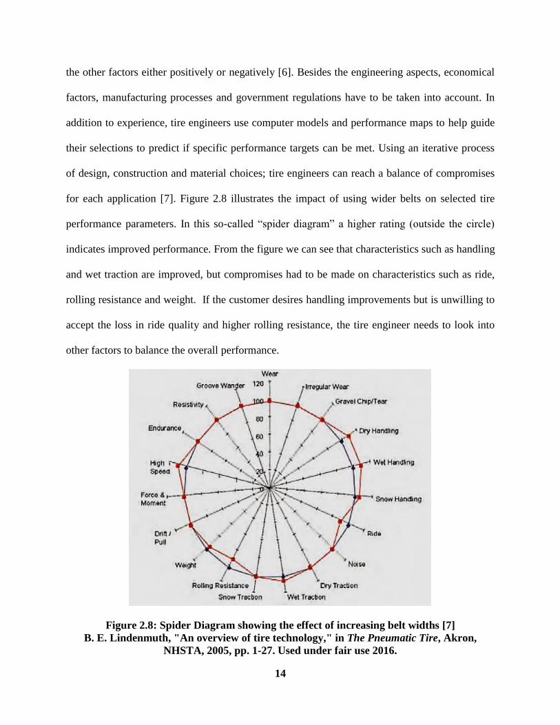
for each application [7]. Figure 2.8 illustrates the impact of using wider belts on selected tire
performance parameters. In this so-called “spider diagram” a higher rating (outside the circle)
indicates improved performance. From the figure we can see that characteristics such as handling
and wet traction are improved, but compromises had to be made on characteristics such as ride,
rolling resistance and weight. If the customer desires handling improvements but is unwilling to
accept the loss in ride quality and higher rolling resistance, the tire engineer needs to look into
other factors to balance the overall performance.
Figure 2.8: Spider Diagram showing the effect of increasing belt widths [7]
B. E. Lindenmuth, "An overview of tire technology," in The Pneumatic Tire, Akron,
NHSTA, 2005, pp. 1-27. Used under fair use 2016.
15
Developing an accurate model that would describe the tire behavior in order to optimize the
overall performance, is very important for the tire industry. For this purpose, several modeling
techniques have been developed during the past few decades. One of the most well-known and
widely used tire handling models is the Magic Formula model of Pacejka [8]. This model is very
useful to reproduce and interpolate tire forces and moments. The great advantage of this model is
the low computational cost. This is a widely used tire model for vehicle dynamics simulations,
where the tire is just one part of the total vehicle model. The main drawback of this this model is
that the parameters are experimentally determined from full scale tire tests and as such these
models cannot be used to predict the influence of tire design changes. For a detailed tire analysis,
Finite Element (FE) Method is very useful. Generally, finite element modeling is quite complex,
but this is a great technique that allows tire engineers to investigate the effects of tire design
parameters on the generated forces and moments. FE models are nowadays a standard tool in the
tire industry, and their use opens the possibility of tire virtual prototyping.
2.5. The footprint phenomena
The tire has essentially 3 contact regions: one with the road and the other two are the contact
regions between the bead areas and the rim [9]. This thesis focuses on understanding what goes
on when the tire is in contact with the road surface or commonly referred to as the footprint
phenomena. Note, that the term “footprint” and “contact patch” are used interchangeably
throughout this thesis. Understanding the tire footprint is a very complex phenomenon. The
study of the tire footprint is a very complex matter for several reasons as noted by Pottinger [10].
They are outlined below:
i. The tire is a doubly curved surface; it has curves in both the circumferential direction and
the transverse or lateral direction. A doubly curved surface is not developable and cannot

16
be conformed to a flat or round surface simply by bending parallel to the tire center
plane. The tire structure needs to be both stretched, compressed and bent as well
ii. The tire is a relatively flexible, pre-stressed structure whose behavior depends on applied
loads and operating conditions.
iii. The friction of the road or test surface, an environmental operating condition, affects the
deformation of the tire and, hence, the tire’s footprint. A deformable road surface affects
the tire footprint.
In spite of these difficulties, the reason a lot of studies have been done on the footprint
phenomena is because of the significant impact it has on functional performance parameters of
the tire such as traction, tire/road interaction noise, ride, handling, and wear. The footprint
physics will be discussed elaborately, in chapter 5 as the experimental and simulation footprint
results can be used as good examples to explain this phenomenon. The following section
discusses the methods and techniques used over the years in order to obtain the tire footprint.
2.6. Pure visualization techniques for footprint measurement
2.6.1. Glass plate photography
This is a good method that has been used over the years to study the footprint shape and
geometry. This method does not provide any information about the stress distribution field at the
contact patch. As noted earlier, the footprint shape greatly influences the tire performance and is
very dependent on its profile or the aspect ratio. Figure 2.9 (a) shows an image of the footprint
obtained when the tire is operating at a positive slip angle at slow rolling speeds in dry
conditions. Along with modern computer-enhanced imaging, this technique can be used to
measure not only basic footprint shapes, but also to determine the tread slip or surface sliding
simultaneously [9].

17
Figure 2.9: Glass plate photography footprint example in (a) dry and (b) wet conditions [9]
M. Pottinger, "Contact Patch (Footprint) Phenomena," in The Pneumatic Tire, Akron,
NHSTA, 2005, pp. 231-286. Used under fair use 2016.
This technique is also very useful for analyzing the footprint under wet conditions to study the
effect of hydroplaning as shown in figure 2.9 (b). A fluorescent dye is introduced into the water
on top of the glass plate [9] to achieve this result.
2.7. Techniques used for footprint stress measurement
Contact between the tire and road leads to a complex distribution of stresses across the footprint
area. The distribution has both a normal component and two shear components at each point in
the footprint. The manner in which these stresses are distributed across the contact patch depend
on several factors which include the normal load acting on the tire, the tire geometry, aspect
ratio, tread profile, belt and cord orientation, tire-road friction and much more. Footprint stress
measurement techniques began with normal stress or pressure determination since the early
1960’s. Since then these techniques have evolved, and can now measure stresses even the lateral
and longitudinal direction at very fine resolutions. This thesis focuses on the normal stress

18
measurement techniques which are discussed in detail in chapter 4. The normal stress and full 3D
stress measurement techniques will be discussed in detail in the following sections.
2.7.1. Normal stress measurement techniques
2.7.1.1. Pressure sensitive film: Fujifilm Prescale
Pressure sensitive films are very useful for measuring contact/normal pressure distributions. It
works on a fairly simple principle. Basically these films carry micro-capsule layers filled with
color, which burst under the application of pressure. The intensity of this color gives an
indication of the maximum pressure that exists in the footprint at a given location. Fujifilm used
this technique to come up with the first commercial product of this type, Prescale, which uses an
encapsulated dye layer on a Mylar/polyester substrate. Figure 2.10 shows the footprint shape and
contact pressure distribution obtained using this technique.
Figure 2.10: Fujifilm Prescale used for contact pressure and footprint shape measurement
Using an appropriate densitometer and software, the maximum (peak) normal pressure can be
determined at each point in the footprint with very good resolution as shown in figure 2.10. This
can be utilized in both the static condition and at slow rolling speeds. Given the simplicity and
cost-effectiveness of this technique it has been utilized for experimental studies presented in this
thesis. A more detailed and in depth explanation about this method is discussed in chapter 4.
19
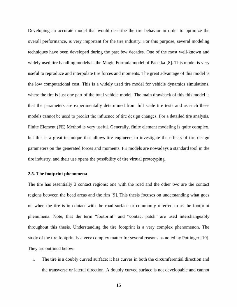
2.7.1.2. Pressure mats: TireScan (TekScan) pressure measuring system
TireScan system is a system developed by TekScan which can be used to capture a static or
dynamic tire footprint patterns using a tactile pressure sensor. Unlike the Fujifilm Prescale, the
TireScan system is capable of recording real-time normal stresses at slow rolling conditions. The
Fujifilm Prescale is only capable of recording the peak stresses as the tire rolls over the surface.
Real-time data is captured, stored, and can be analyzed using a wide range of application specific
graphs, imaging analysis tools [11].
Figure 2.11: Footprint contact pressure analysis using the TekScan system [11]
TekScan, "TireScan CrossDrive System," [Online]. Available:
https://www.tekscan.com/products-solutions/systems/tirescan-crossdrive-system. [Accessed
03 09 2016]. Used under fair use 2016.
Recent developments to the TireScan system has enabled shear stress measurements using the
TireScan Cross-drive system, which uses over 250000 sensing elements which are resistive in
nature. However, this system is very expensive in comparison with the Fujifilm Prescale system.

20
2.7.1.3. Optical method: Frustrated total internal reflectance
Another method used to obtain the normal pressure distribution is by an optical method
commonly referred to as “Frustrated Total Internal Reflectance”. Note that this method has not
been used for the experimental procedure described later on in chapter 4; this is only a review of
literature. It works on a fairly simple principle. Basically, light shines through glass plate from its
edges at particular angle such that nothing touches the surface of the plate. The light is
essentially totally reflected within the plate at that angle. The light cannot pass from the glass
back into the air except for limited leakage associated with the presence of an electrical
disturbance in the air [12].
Figure 2.12: Frustrated Total Internal Reflectance [12]
C. R. Gentle, "Optical Mapping of Pressures in the Tyre Contact Patch," Optics and Lasers
in Engineering, vol. 4, pp. 167-176, 1983. Used under fair use 2016.
If a third medium with a high optical density is introduced at the interface, the presence of the
light from this medium will be partially transmitted across the interface. The total internally
reflected light will be frustrated, and an illuminated spot would appear in the field as shown in
figure 2.12. Generally, a thin vinyl sheet or a tablecloth with small holes is introduced between

21
the test tire and the glass to achieve this purpose. The brightness of the illuminated spot at each
hole depends on the amount of contact at each location. The magnitude of contact depends on
how firmly the sheet is pressed against the glass, and thus the pressure distribution field is
interpreted as a function of the brightness level. Using a video camera and appropriate software,
high resolution pressure images can be produced as shown in figure 2.13
Figure 2.13: Contact Pressure Footprint using Frustrated Total Internal Reflectance [12]
C. R. Gentle, "Optical Mapping of Pressures in the Tyre Contact Patch," Optics and Lasers
in Engineering, vol. 4, pp. 167-176, 1983. Used under fair use 2016.
2.7.2. 3D-stress Measurement Technique
2.7.2.1. 3D Force transducer arrays
This is the only technology that allows determination of contact pressure in addition to the two
shear stresses, using 3-D force transducers. This has been elaborately discussed by Pottinger in
[9]. Note that this method has not been used for the experimental procedure described later on in
chapter 4; this is only a review of literature. Figure 2.14 shows a schematic representation of a
miniature force transducer installed in a test surface. Using a single transducer, of course has its
limitations, as it can only measure the stress data at a single point along the length of the

22
footprint. As we need to get the stress distribution across the entire footprint, data needs to be
taken at multiple tread points. This requires an array of transducers as shown in figure 2.15.
Figure 2.14: Miniature force transducer installed in a test surface [9]
M. Pottinger, "Contact Patch (Footprint) Phenomena," in The Pneumatic Tire, Akron,
NHSTA, 2005, pp. 231-286. Used under fair use 2016.
Figure 2.15: 3D Force transducer arrays [9]
M. Pottinger, "Contact Patch (Footprint) Phenomena," in The Pneumatic Tire, Akron,
NHSTA, 2005, pp. 231-286. Used under fair use 2016.
23
3.
THE TIRE FINITE ELEMENT
MODELING PROCESS
3.1. Introduction
As mentioned in chapter 1, finite element modeling is a very useful tool that is used in tire
development. Finite element tire modeling can significantly predict the influence of tire design
changes which vastly helps reduce tire development time. As stated earlier, one of objectives of
this thesis is develop a finite element tire model (of a specific tire) through an in-house reverse
engineering process, and compare the accuracy of the simulation results against experimental test
data. Numerical modeling of a tire in combination with its environment is a challenging task.
Typically the mechanical, thermal and fluid domains contribute to the tire response. This
research is restricted to the mechanical domain in which a numerical modeling framework for
steady-state rolling tire simulations is defined. In this chapter the methods, procedure and
techniques used in tire finite element modeling are presented. First a brief overview of the
challenges in the tire finite element modeling process, the methods and the steady state transport
analyses capabilities in ABAQUS are outlined. The in-house developed reverse engineering
process used to create the finite element tire model is then discussed in detail.

24
3.2. Challenges in the finite element tire modeling process
As mentioned earlier, numerical modeling of a tire in combination with its environment is a
difficult task. Some of the challenges in the FE modeling process specific to the scope of this
thesis has been outlined below:
i. Material modeling: Properly characterizing the materials used in the tire is critical in the
finite element tire modeling process. As the tire is highly non-linear in nature, the type of
material model used has a significant impact on the simulation results. Large
deformations and large strains, as well as the near-incompressibility of rubber compounds
should be accounted for. An accurate description of the various rubber compounds in the
tire, details about the plies, belts and cords are very important as well.
ii. Contact/friction modeling: The type of contact model used between the tire and road
has a significant impact on the contact patch phenomena. There are several different
contact models that have been developed over the years, and this will be looked in much
greater detail in later sections in this chapter.
iii. Geometric modeling: As this entire thesis is based on the contact patch phenomena,
getting an accurate depiction of the 2D-cross sectional geometry details of the tire are
very crucial as well. Especially since the 2D layout of the test tire has not been provided,
accurately representing the 2D profile of the tire has been very challenging.

25
3.3. Finite Element Analysis Methods for Tires
There are three types of finite element methods generally used in tire modeling. They are briefly
outlined below:
3.3.1. Implicit dynamic method
An implicit analysis is solved using an incremental-iterative procedure, which requires matrix
inversion [13]. These types of analyses are generally used when inertia effects can be neglected
and time-dependent material effects are not included. In this case the time increments are then
simply fractions of the total period of the step, which are used as increments in the analysis. If
time dependent material effects are taken into account, such as viscoelastic materials, the
approach is called “quasi-static”. An implicit dynamical analysis is not often used for rolling
tires, since it is well-known that this type of analysis is not efficient in solving changing contact
conditions. The nonlinear equation solving process is expensive due to the Newton iterations,
and if the equations are very nonlinear, as in the case of changing contact, it may be difficult to
obtain a solution [13].
3.3.2. Arbitrary Lagrangian-Eulerian method
The arbitrary Lagrangian-Eulerian (ALE) method is developed for numerical analysis of rolling
contact problems [14]. This method converts the steady state moving contact problem into a pure
spatially dependent simulation, where the mesh is fixed in space and the material flows trough
the mesh. Thus the mesh needs to be refined only in the contact region, which leads to a
computational time reduction. This will be discussed further in section 3.4.
26
3.3.3. Dynamic Explicit Analysis:
In an explicit analysis the dynamic response problems are solved using an explicit direct
integration procedure. The displacements and velocities are calculated in terms of quantities that
are known at the beginning of an increment. No iterations and no tangent stiffness matrices are
required, which is an advantage compared to the implicit method. However due to the explicit
time integration, a very small time-step which depends on the highest frequency present in the
model, is usually required. Explicit dynamic analysis in ABAQUS is quite useful for the
analysis of rolling and sliding contact between a tire and a road surface. In this approach the
reference frame is associated with the material. Explicit dynamic analysis is a pure Lagrangian
finite element method in which steady-state rolling of a tire is a time dependent process [15]. It is
a computationally expensive method, considering that a small time increment may be necessary
in the analysis. Costs increase with tire rolling speed. Therefore this approach is ideal to simulate
transient behavior in a short time span, such as impact of a tire with a cleat. It can also be used to
compute handling characteristics, but longer time spans are required to reach the steady-state
situation. Furthermore for these longer time spans the risk of error accumulation is present as
shown by Rao in [16].
3.4. Steady State Transport Capabilities using ABAQUS
Steady-state transport analysis in ABAQUS is used for analysis of rolling and sliding contact
between a tire and a flat, convex or concave road. This is very elaborately discussed in the
ABAQUS documentation [13]. A very brief overview is summarized in this section. In this
approach the reference frame is attached to the axle. An observer in this reference frame
perceives points on the tire to be stationary; the tire material moves through the points. Thus, the
tire finite element model does not undergo large rigid body rotation. Deformation is calculated

27
relative to rotation using steady-state transport analysis that is a mixed Lagrangian / Eulerian
finite element method. Rigid body motion is analyzed using an Eulerian approach and
deformation is analyzed using a Lagrangian approach. It is an inexpensive method, especially
considering that its costs are independent of tire rolling speed. Koishi [17] made a comparison
between the steady-state transport method, ABAQUS/Explicit method and experimental tests for
steady-state cornering maneuvers. Although the results of both FE methods are closer to each
other than to the experiments, the steady-state transport method is significantly faster, 6 hours
and 8 days respectively. This, together with the possibility to reduce the number of elements
outside the contact area, clearly shows the benefits of the steady-state transport analysis and
therefore this method is chosen to compute the steady-state characteristics of a rolling tire.
3.5. Tire Finite Element Modeling Procedure
The tire finite element model was created and solved in ABAQUS version 6.14-3. This section
discusses the methods, techniques and reverse engineering principles followed to create this
finite element tire model.
3.5.1. Creation of the 2D Cross Section of the Tire Model in ABAQUS
The first step is perhaps the most crucial and important step in the entire tire modeling process.
Every single feature geometric feature such as the tread radii, sidewall radii, belt and cord
positions, their orientation, bead geometry and the like, have a significant impact on the overall
shape of the footprint and pressure distribution. The tire modeled is a Michelin P205/60 R15
91H. Without an accurate representation of the 2-D cross section of the tire, it would be
impossible for the experimental and simulation footprints results to concur with each other.
Unfortunately most tire companies keep this data confidential, so an in-house reverse
28
engineering process had to be developed in order to create an accurate 2D-geometric model. The
following section describes the reverse engineering process.
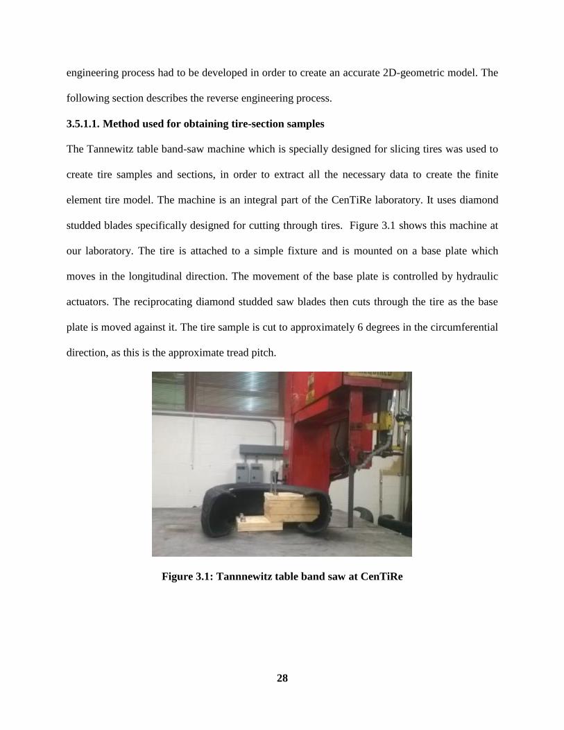
3.5.1.1. Method used for obtaining tire-section samples
The Tannewitz table band-saw machine which is specially designed for slicing tires was used to
create tire samples and sections, in order to extract all the necessary data to create the finite
element tire model. The machine is an integral part of the CenTiRe laboratory. It uses diamond
studded blades specifically designed for cutting through tires. Figure 3.1 shows this machine at
our laboratory. The tire is attached to a simple fixture and is mounted on a base plate which
moves in the longitudinal direction. The movement of the base plate is controlled by hydraulic
actuators. The reciprocating diamond studded saw blades then cuts through the tire as the base
plate is moved against it. The tire sample is cut to approximately 6 degrees in the circumferential
direction, as this is the approximate tread pitch.
Figure 3.1: Tannnewitz table band saw at CenTiRe

29
3.5.1.2. Determining the tire mounting position on rim
Once the tire section has been obtained, it is very important to determine the exact mounting
position of the tire on the rim. The distance from each end of the rim was measured precisely.
Figure 3.2: Tire Section mounted on rim to obtain end to end distance
Figure 3.2 shows the cut tire section mounted on the rim. Using this information, the distance
from each end of the tire was measured accurately using measuring tape. In this case a 15 inch
rim of a Volkswagen Jetta was used as this is the same rim that is used in the experimental setup
as well.
3.5.1.3. Tire profile measurement techniques
As mentioned earlier, it is very important to obtain precise geometry details of each feature of
the tire profile. This includes the sidewall dimensions, carcass dimensions and the tread
dimensions including the tread radii, shoulder radii and tread depth to name a few. In order to
measure entire outer profile of the tire accurately, a special profile measuring tool known as a
“contour gauge” is used. Figure 3.3 shows the contour gauge that was used for this purpose. It
typically consists of steel “bristles”, which can conform to the silhouette of a complex shape of
an object, with the application of pressure. It is to be noted that as the 2D finite element model is

30
created in the uninflated state initially, it is critical to ensure that the dimensions of the profile
obtained are also in the uninflated state.
Figure 3.3: Contour gauge used for tire profile measurement
For this reason the tire was inflated to about 3 PSI, so that tire bead ends have just enough
pressure to just stick to the surface of the rim. Figures 3.4 and 3.5 show the measured tread
profile and the sidewall profile of the tire in the uninflated state respectively.
Figure 3.4: Tread profile measurement (one-half of tread) using the contour gauge

31
Figure 3.5: Sidewall profile measurement using the contour gauge
Using the contour gauge as a reference for the tire outer profile, the sample tire section was
accurately positioned on a flat polycarbonate sheet using strong duct tape (gorilla tape) to
constrain the tire boundary such that it represents actual mounting position of the tire on the rim
in the uninflated state. Note that this tire section was finely ground, to ensure that both surfaces
of the tire section were as flat as possible. Figure 3.6 shows the processed image of the tire cross
section using the specially calibrated Topaq scanner in order to get a high resolution image of the
tire cross section.

32
Figure 3.6: Processed high resolution tire cross section image
3.5.1.4. Converting the processed image into in 2-D ABAQUS tire model
Once the high resolution image of the tire cross section with its exact location, orientation and
position on the rim is obtained as described in section 3.5.1.3, it can then be imported in into
ABAQUS, where it can be used as a reference to create the 2D tire model. Figure 3.7 shows the
sketched tire cross section using the processed image as a reference. The processed image had to
be scaled accordingly in ABAQUS in order to make sure that the dimensions of the tire profile
corresponded to the actual dimensions. Care had to be taken to ensure that every radius and
curvature was measured as accurately as possible. This 2D- cross section is the foundation on
which the entire finite element model is built.

33
Figure 3.7: Tire cross-section (one-half) ABAQUS sketch created from processed image
3.5.2. Tire reinforcements geometric and material characterization
The test tire is essentially a 4 ply tire, which includes a carcass ply, 2 steel belts and a polyamide
cap ply. Small tire samples were sliced in order to analyze reinforcement elements more closely.
Figure 3.8 show few of the sliced tire samples. From left to right, figure 3.8 (a) shows the steel
belts; figure 3.8 (b) shows the carcass plies and figure 3.8 (c) shows the polyamide cap plies.
These sections were analyzed closely under a microscope to get accurate values for geometric
properties of the reinforcement elements.
Figure 3.8: Sliced tire samples: Steel belts (a), carcass plies (b) and cap plies (c)

34
Some of the key parameters to be measured include the spacing between each belt, carcass and
polyamide (nylon) cap plies, individual spacing between each belt, carcass ply and cap ply, the
orientation of each of these elements and the diameter of each individual element. The following
table 3.1 summarizes the measured geometric properties for the reinforcement elements.
Table 3.1: Measured geometric properties for reinforcement elements
Element Measured
Diameter (mm)
Effective Area
(mm2)
Spacing
(mm)
Orientation
(degrees)
Steel Belts
(Upper &
Lower)
0.38 0.2268 1.33 66.3, -66.3
Carcass
Ply 0.5 0.1963 0.9 0
Nylon
Cap Ply 0.6 0.2827 0.98 90
Note that the orientation of these elements is taken with respect to the horizontal axis
perpendicular to the circumferential direction of the tire. Generally in order to determine the
material properties of these reinforcement elements, experimental tests are generally conducted
based on specific standards, such as ASTM standard D885/D885M. Performing simple tensile
tests using Dynamic Mechanical Analyzer (DMA) is also another way of determining the elastic
properties of the belts and cords. However obtaining clean samples for each of these
reinforcement elements was extremely difficult as they are fused along with the other rubber
compounds. After extensive research, it was found that using the elastic properties of the
reinforcement elements used by Balaramakrishna et. Al in [18] seemed to provide accurate
results in comparison with the experimental test data. The following table 3.2 summarizes the
elastic properties used.

35
Table 3.2: Material properties for reinforcement elements used
Element Poisson's Ratio Density (kg/m3) Elastic Modulus (MPa)
Steel Belt 0.33 7.62E+03 2.18E+05
Carcass Ply 0.49 1.07E+03 4.94E+03
Nylon Cap Ply 0.49 9.40E+02 2.20E+03
3.6. Tire Material Model Selection
As the tire is a composite material, it has complex characteristics due to its diverse material
properties and complex structure. As mentioned in chapter 2, the tire consists of different rubber
components with embedded reinforcements. Some of the components include the tread, under-
tread, sidewall, apex, and the inner-liner. The rubber material properties for different components
such as tread and sidewall are not identical due to the different mixed proportions of rubber and
carbon black [2]. They have different characteristics to meet the different functional
requirements. For example, the function of tread rubber is to keep the balance of tire
performance and durability, while the sidewall rubber is designed mainly for fatigue resistance
[2]. Rubber has flexible and long molecular structures, which enables it to elongate to several
times its original size. For some simple cases, the assumption of a linear stress-strain relationship
can be used to represent the rubber material property. As with other solid materials, rubber can
be considered as a linearly elastic material at small strains. This assumption can cover some
common rubber design problems. However, for analyzing rubber behavior under large
deformation, large elastic deformation theory should be considered [19]. Taking this into
consideration, various hyper-elastic models have been developed over the years to describe
rubber material behavior, based on continuum mechanics. The selection of a proper strain energy
function W is very important in the modelling process of a hyper-elastic rubber material.

36
Determining accurate material constants for the selected function is also of great importance.
Generally the strain energy functions can be represented as follows:
𝑾 = 𝒇(𝑰𝟏, 𝑰𝟐, 𝑰𝟑) (3.1)
Where:
𝑊= Strain energy potential (density) or stored energy function defined per unit volume.
𝐼1, 𝐼2, 𝐼3= Three invariants of the Cauchy-green tensor given in terms of the principal extension
ratios 𝜆1, 𝜆2, 𝜆3, where
𝑰𝟏 = 𝝀𝟏𝟐 + 𝝀𝟐
𝟐 + 𝝀𝟑𝟐 (3.2)
𝑰𝟐 = 𝝀𝟏𝟐𝝀𝟐
𝟐 + 𝝀𝟐𝟐𝝀𝟑
𝟐 + 𝝀𝟑𝟐 𝝀𝟏
𝟐 (3.3)
𝑰𝟑 = 𝝀𝟏𝟐𝝀𝟐
𝟐𝝀𝟑𝟐 (3.4)
As described from Chagnon [20] an efficient and reliable hyper-elastic model has four main
qualities:
i. It should be able to exactly reproduce the whole responses of rubber in an expected ‘S’
shape.
ii. The change of deformation modes must be reasonable. For instance, if the model operates
sufficiently in uniaxial tension, it must also be exact in simple shear or in equi-biaxial
tension without an obvious problem.
iii. The number of fitting material parameters should not be large, so the number of
experimental tests for their determination can be reduced.
iv. The mathematical formulation of the strain energy potential should also be simple and
practicable for the numerical performance of the model.

37
The Neo-Hookean hyper-elastic material model was selected as it has the ability to reasonably
depict the hyper-elastic characteristics of rubber at low strain levels. It is also a rather simple
model, which requires just two fitting parameters as inputs: the shear modulus and the bulk
modulus of the material. As performing DMA tests for the rubber components is not within the
scope of this thesis, these properties are derived from the Young’s modulus, which in turn can be
easily derived from material hardness tests.
Besides this, the Neo-Hookean model is built into ABAQUS, which makes it very convenient.
The Neo-Hookean model would have the ability to represent the non-linear nature of the rubber
at smaller strains, than say, a linear elastic model. However the problem with the Neo-Hookean
model is that it does not have the ability to predict the response of rubber at higher strain levels
(beyond the upper-knee of the “S-Curve”). The maximum strain level seen at 120 slip was found
to 19%. The neo-Hookean model may be able to predict the response at these strain levels
reasonably; however it is very important to note that in order to accurately predict the response,
full-scale material testing would need to be performed.
The strain energy function for Neo-Hookean model is given by:
𝑾 = 𝑪𝟏𝟎(𝑰�̅� − 𝟑) + 𝟏
𝑫𝟏(𝑱𝒆𝟏̅̅ ̅̅ − 𝟑)𝟐 (3.5)
Where:
𝐶10= Constant describing the shear modulus G = 𝐺
2
𝐷1 = Constant describing the bulk modulus K= 2
𝐾
𝐼1̅ = The first invariant of the deviatoric strain tensor
𝐽𝒆1̅̅̅̅ = The elastic volume ratio
The next section describes the method used to obtain the tire material properties.

38
3.7. Method used for obtaining the tire material properties
In order to obtain the constants 𝐶10 & 𝐷1 described in the previous section it is important to
determine the shear modulus and the bulk modulus for each rubber compound. The shear
modulus G and the bulk modulus K can be determined easily if the Young’s modulus E and the
Poisson’s ratio 𝜈 for the rubber compound are known. The shear modulus G is related to the
young’s modulus E by the following relation:
𝑮 (𝑴𝑷𝒂) = 𝑬𝟐(𝟏 + 𝝂)⁄ (3.6)
The bulk modulus K and the Young’s modulus for the material are related by the following
expression:
𝑲 = 𝑬𝟑(𝟏 − 𝟐𝝂)⁄ (3.7)
The Young’s modulus for the material can be easily determined through a simple Shore-A
hardness test. The following semi-empirical equation described by Gent A.N. [21], relates the
Young’s modulus to the indentation hardness value:
𝑬 (𝑴𝑷𝒂) = 𝟎. 𝟎𝟗𝟖𝟏(𝟓𝟔 + 𝟕. 𝟔𝟔𝑺)
𝟎. 𝟏𝟑𝟕𝟓𝟎𝟓(𝟐𝟓𝟒 − 𝟐. 𝟓𝟒𝑺)⁄ (3.8)
Where:
𝑆 =Shore-A hardness value
The shore-A hardness value for each individual rubber compound was determined using a Shore-
A durometer as shown in figure 3.9. It is important to note that this empirical formula is derived
using a particular tire compound. It only gives an approximate value for the Young’s modulus
for the rubber compounds listed in table 3.3. In order to actually determine the hyper-elastic
properties of the various tire compounds, DMA testing would need to be done. The various
deformation modes in tension, compression and shear of the rubber compounds would have to be

39
excited in order to accurately predict the non-linear behavior of the rubber components.
However, this type of testing is not within the scope of this thesis.
Figure 3.9: Fowler Shore-A durometer
The indenter would be pressed against each individual material compound within the sliced tire
sections, and the hardness values would be determined. Figure 3.10 shows the Shore-A
durometer pressed down against the Apex portion of the sample tire section. Multiple readings
were taken at different points within each compound and the average for each reading is noted in
table 3.3. Although multiple readings were taken at each point, this method just provides the
surface hardness for the material. The shore-A hardness test complies with the ASTM D 2240-86
standards and the test was carried out at an ambient temperature of 23𝑜 C.

40
Figure 3.10: Shore-A durometer used to measure hardness value for the apex compound
Table 3.3: Material properties determined from Shore-A hardness test
Element Shore-A
Hardness
Youngs
Modulus
(MPa)
Poisson's
Ratio
Shear
Modulus
(MPa)
Bulk
Modulus
(MPa)
C10
(MPa)
D1
(2/
MPa)
Carcass 52 2.658 0.49 0.892 44.308 0.446 0.045
Sidewall 43 1.899 0.49 0.637 31.650 0.318 0.063
Rim
Strip 70 5.545 0.49 1.860 92.408 0.930 0.021
Belt 72 6.094 0.49 2.045 101.570 1.022 0.019
Tread 63 4.088 0.49 1.371 68.141 0.685 0.029
Apex
(Filler) 90 20.936 0.49 7.025 348.943 3.512 0.006

41
3.8. Tire reinforcement modeling in ABAQUS
The processed 2D tire cross-section image (discussed in section 3.5.1.3) was used as a reference
again in order to locate and position the reinforcement elements in ABAQUS accurately. Figure
3.11 shows all the reinforcement elements modeled in ABAQUS.
Figure 3.11: Reinforcement elements modeled in ABAQUS
Figure 3.12: Reinforcement element details

42
Generally, there exist two methods for modeling reinforced-rubber composites: laminated shell
model and rebar model [22]. The rebar layer function in ABAQUS provides the support for
modelling belts and cords as rebar element which is embedded in rubber solid element as shown
in Figure 3.13
Figure 3.13: Reinforced rubber modeling used rebar elements [22]
Y. Guan, G. Zhao and G. Cheng, "Influence of Belt Cord Angle on a Radial Tire under
Different Rolling States," Journal of Reinforced Plastics and Composites, vol. 25, no. 10, pp.
1059-1077, 2006. Used under fair use 2016.
Material properties of different components obtained from table 3.3 were then applied to the
model. The reinforcement components were modeled using the SFMGAX1 element with 2
nodes, which is embedded in rubber elements in ABAQUS. While meshing, care had to be taken
to ensure that each element normal pointed in the same direction as the others. The geometric
properties of these rebar elements are defined previously in table 3.1. Element and node sets
were created in ABAQUS for different components in order to assign the necessary material
properties and boundary conditions.

43
3.9. Creation of the various tire sections/partitions
The processed 2D tire cross-section image (discussed in section 3.5.1.3), the tire was partitioned
as shown in figure 3.14 in ABAQUS. Partitioning the geometry in an efficient manner is critical
in order to get a good mesh for the model.
Figure 3.14: The different rubber compounds/sections of test tire
If elements have bad aspect ratios, this could result in distortion of elements later on when
running steady state simulations when the effect of inertia is included.
3.10. Element types used and Meshing Techniques for tire geometry
All three element types were tried, CGAX4, CGAX4R and CGAX4H and experimented with.
The hybrid element CGAX4H would generally be useful when a Poisson’s ratio of 0.5 is used,
i.e. when the rubber is considered at “fully-incompressible”. However in this case the rubber is
modeled as “nearly-incompressible” with a Poisson’s ratio of 0.49. The CGAX4H element type
allows for the extra hydrostatic pressure degree of freedom to be accounted for, which generally
results in a non-singular global stiffness matrix. It also requires a longer computational time. The
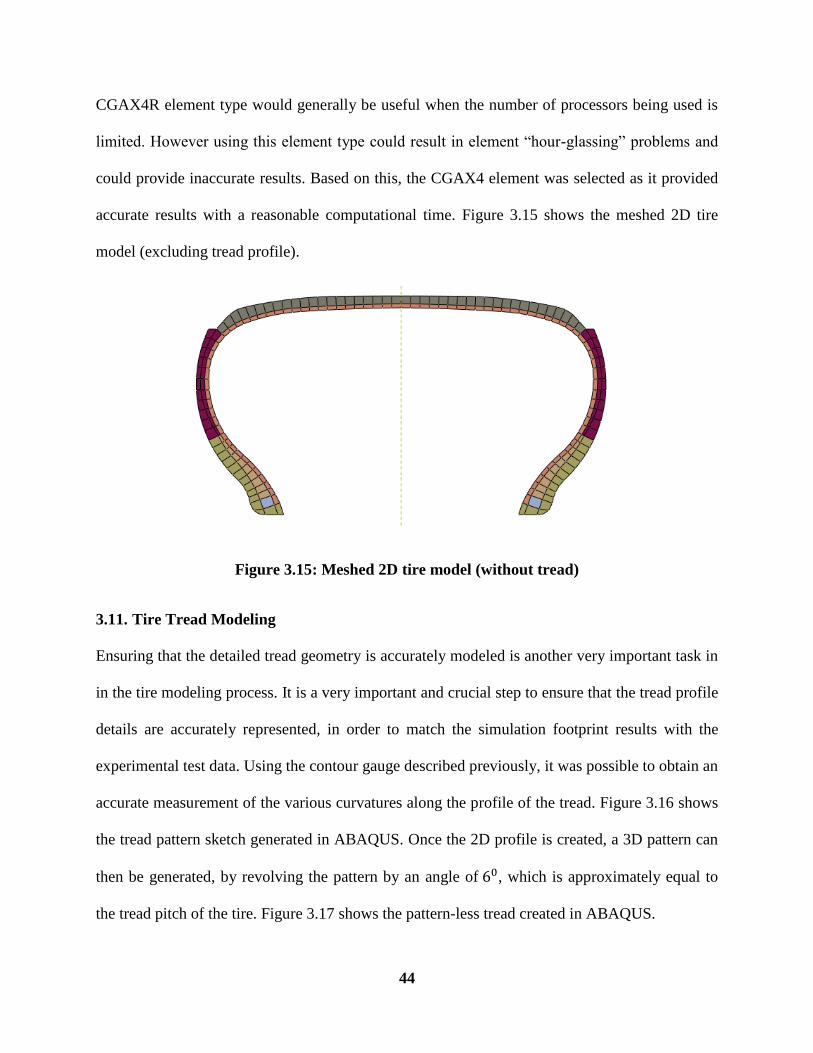
44
CGAX4R element type would generally be useful when the number of processors being used is
limited. However using this element type could result in element “hour-glassing” problems and
could provide inaccurate results. Based on this, the CGAX4 element was selected as it provided
accurate results with a reasonable computational time. Figure 3.15 shows the meshed 2D tire
model (excluding tread profile).
Figure 3.15: Meshed 2D tire model (without tread)
3.11. Tire Tread Modeling
Ensuring that the detailed tread geometry is accurately modeled is another very important task in
in the tire modeling process. It is a very important and crucial step to ensure that the tread profile
details are accurately represented, in order to match the simulation footprint results with the
experimental test data. Using the contour gauge described previously, it was possible to obtain an
accurate measurement of the various curvatures along the profile of the tread. Figure 3.16 shows
the tread pattern sketch generated in ABAQUS. Once the 2D profile is created, a 3D pattern can
then be generated, by revolving the pattern by an angle of 60, which is approximately equal to
the tread pitch of the tire. Figure 3.17 shows the pattern-less tread created in ABAQUS.
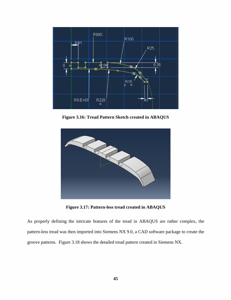
45
Figure 3.16: Tread Pattern Sketch created in ABAQUS
Figure 3.17: Pattern-less tread created in ABAQUS
As properly defining the intricate features of the tread in ABAQUS are rather complex, the
pattern-less tread was then imported into Siemens NX 9.0, a CAD software package to create the
groove patterns. Figure 3.18 shows the detailed tread pattern created in Siemens NX.

46
Figure 3.18: Complete tread pattern sector created in NX
The pattern was then imported back into ABAQUS where it is meshed using 8-noded brick
elements C3D8R, which includes enhanced hourglass control and reduced integration. It’s
important to note that the C3D8R element type was chose in order to reduce computational time.
The C3D8 (full-integration) element type would provide more accurate results especially in for
the shear stresses at the contact patch as it better describes the deformation modes of the
material. Figure 3.19 shows the completed mesh. Care had to be taken to ensure that the
geometry was appropriately partitioned, in order to get a good structured mesh.
Figure 3.19: Meshed Tread geometry using element type CD38R
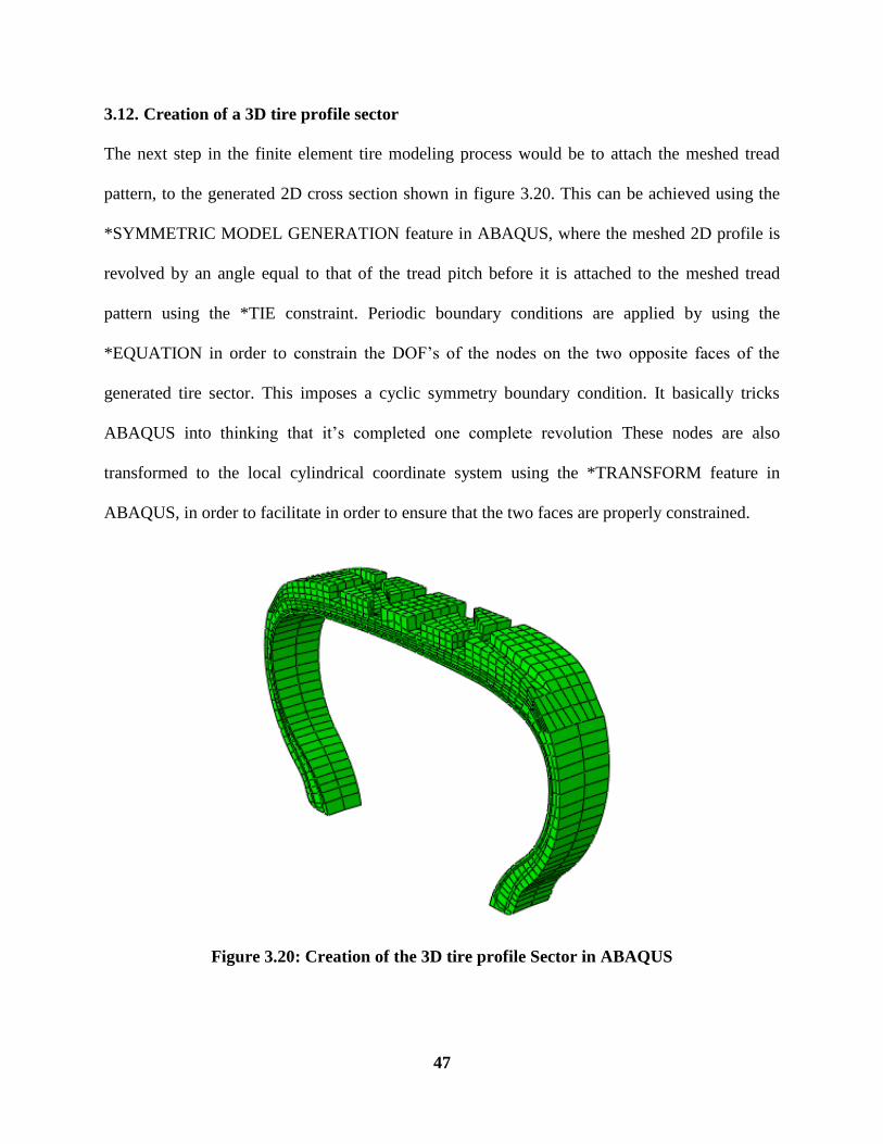
47
3.12. Creation of a 3D tire profile sector
The next step in the finite element tire modeling process would be to attach the meshed tread
pattern, to the generated 2D cross section shown in figure 3.20. This can be achieved using the
*SYMMETRIC MODEL GENERATION feature in ABAQUS, where the meshed 2D profile is
revolved by an angle equal to that of the tread pitch before it is attached to the meshed tread
pattern using the *TIE constraint. Periodic boundary conditions are applied by using the
*EQUATION in order to constrain the DOF’s of the nodes on the two opposite faces of the
generated tire sector. This imposes a cyclic symmetry boundary condition. It basically tricks
ABAQUS into thinking that it’s completed one complete revolution These nodes are also
transformed to the local cylindrical coordinate system using the *TRANSFORM feature in
ABAQUS, in order to facilitate in order to ensure that the two faces are properly constrained.
Figure 3.20: Creation of the 3D tire profile Sector in ABAQUS
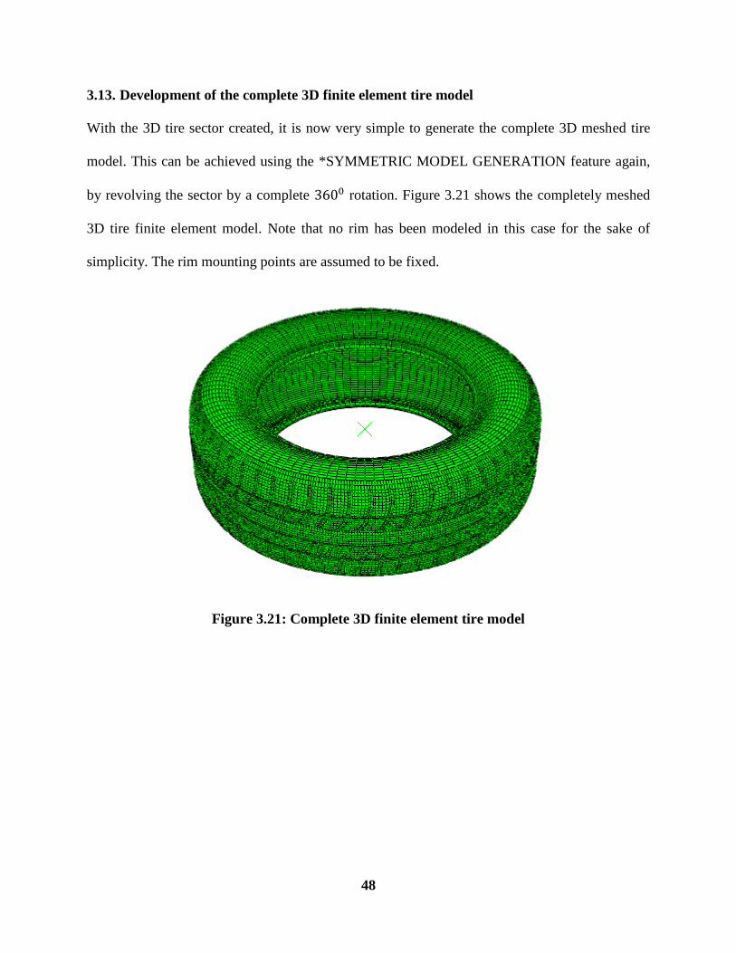
48
3.13. Development of the complete 3D finite element tire model
With the 3D tire sector created, it is now very simple to generate the complete 3D meshed tire
model. This can be achieved using the *SYMMETRIC MODEL GENERATION feature again,
by revolving the sector by a complete 3600 rotation. Figure 3.21 shows the completely meshed
3D tire finite element model. Note that no rim has been modeled in this case for the sake of
simplicity. The rim mounting points are assumed to be fixed.
Figure 3.21: Complete 3D finite element tire model
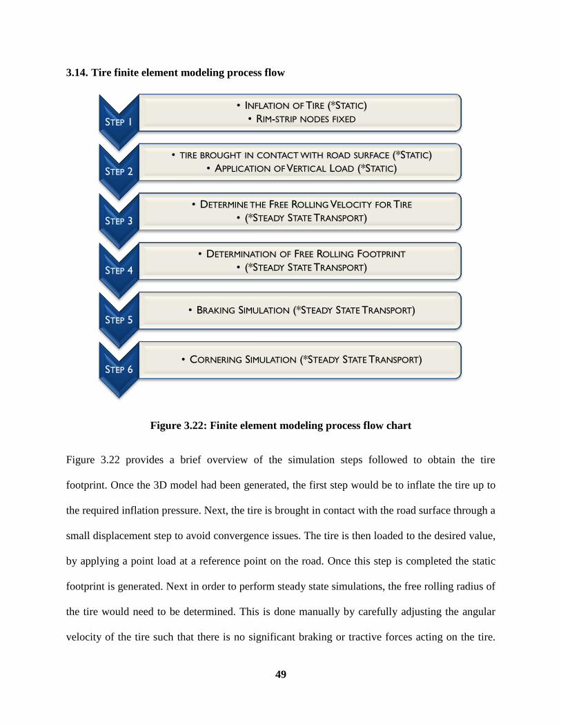
49
3.14. Tire finite element modeling process flow
Figure 3.22: Finite element modeling process flow chart
Figure 3.22 provides a brief overview of the simulation steps followed to obtain the tire
footprint. Once the 3D model had been generated, the first step would be to inflate the tire up to
the required inflation pressure. Next, the tire is brought in contact with the road surface through a
small displacement step to avoid convergence issues. The tire is then loaded to the desired value,
by applying a point load at a reference point on the road. Once this step is completed the static
footprint is generated. Next in order to perform steady state simulations, the free rolling radius of
the tire would need to be determined. This is done manually by carefully adjusting the angular
velocity of the tire such that there is no significant braking or tractive forces acting on the tire.
STEP 1
• INFLATION OF TIRE (*STATIC)
• RIM-STRIP NODES FIXED
STEP 2
• TIRE BROUGHT IN CONTACT WITH ROAD SURFACE (*STATIC)
• APPLICATION OF VERTICAL LOAD (*STATIC)
STEP 3
• DETERMINE THE FREE ROLLING VELOCITY FOR TIRE
• (*STEADY STATE TRANSPORT)
STEP 4
• DETERMINATION OF FREE ROLLING FOOTPRINT
• (*STEADY STATE TRANSPORT)
STEP 5 • BRAKING SIMULATION (*STEADY STATE TRANSPORT)
STEP 6 • CORNERING SIMULATION (*STEADY STATE TRANSPORT)

50
Ideally, the free rolling velocity would be the velocity at which the longitudinal forces are 0, but
this is very difficult to achieve. Having a longitudinal force within ±50N is reasonably
acceptable. Once the free rolling radius/velocity has been determined, the free rolling simulation
can then be run to obtain the 3D stress distribution field at the contact patch. Once this step has
been completed, it is possible to run braking, traction, cornering, combined slip or simulations
including the effect of camber. However running these simulations at high rotational speeds and
slip angles, using ABAQUS’ default friction model has not been fruitful as it has resulted in the
problem of excessive distorted elements in the contact region. This will be looked at closely in
the following section.
3.15. Contact modeling problem in ABAQUS during steady state rolling
3.15.1. Coulomb’s classical friction model
As mentioned in the previous section ABAQUS uses Coulomb’s classical friction model by
default for solving contact problems using the steady state transport capability. Figure 3.23
shows a representation of Coulombs classical friction model. There are two possible conditions:
a “slip” condition and a “stick” condition. The “stick: condition is said to exist if:
𝝉 ≤ 𝝉𝒄𝒓𝒊𝒕 (3.9)
Where:
𝜏𝑐𝑟𝑖𝑡 = Critical shear stress = 𝜇𝑝;
𝑝 = Contact pressure,
𝜏 = Shear stress at a particular node
The condition is said to be in the “slip” condition if 𝜏 exceeds the critical shear stress 𝜏𝑐𝑟𝑖𝑡.

51
This constraint can be handled in ABAQUS in two different ways, using a Lagrange multiplier or
by using a regularization step. In case of the Lagrange multiplier method, the constraint is
obeyed exactly, however the additional multipliers increase the cost of the analysis and
convergence problems may occur in areas where the contact conditions change [13]. A
regularization step is chosen in order to avoid the non-differentiability of Coulomb’s law at zero
slip velocity. The regularization function is chosen such that the transition from stick to slip is
smooth. However this regularized function has the drawback that the transition from stick to slip
is approximated.
Another important drawback of the classical Coulomb friction model is that it does not take the
relation between contact pressure and friction into account. Using a constant friction model the
problem of excessive distorted elements around the tread region in contact with the surface,
could result in convergence issues and inaccurate results.
Figure 3.23: Classic Coulomb’s law (a) and regularized functions of Coulombs law (b) [23]
R. V. D. Steen, "Tire-Road Friction Modeling," Eindhoven University of Technology ,
2007. Used under fair use 2016.
3.15.2. Pressure dependent friction model
In order to over the drawbacks of the classical Coulomb model a pressure dependent friction
model has been implemented. This friction model is an extension to Savkoor’s friction model has

52
been implemented. Savkoor [24] proposed a model where he described the friction as a function
of slip velocity 𝜇(𝑣) with an empirical relation given below:
𝝁(𝒗) = 𝝁𝒔 + (𝝁𝒎 − 𝝁𝒔)𝒆−𝒉𝟐 𝐥𝐨𝐠𝟐 𝒗/𝑽𝒎𝒂𝒙 (3.10)
Where:
𝜇𝑠= Static coefficient of friction
𝜇𝑚= peak value of friction (when 𝑣 = 𝑣𝑚𝑎𝑥)
ℎ = Dimensionless parameter reflecting the width of the speed range, in which friction varies
𝑣 = Sliding velocity of the point/block
𝑉𝑚𝑎𝑥= Sliding velocity at peak friction.
Figure 3.24: Friction model proposed by Savkoor [23]
R. V. D. Steen, "Tire-Road Friction Modeling," Eindhoven University of Technology ,
2007. Used under fair use 2016.
Savkoor’s model is chosen to describe the sliding velocity dependence, since the parameters in
this model are directly related to the shape of the friction curve. It is shown by Lupker [25], that
this model can also be used in situations with very high sliding velocities.
Although Savkoor’s model does provide a more realistic representation of how rubber friction
varies with sliding velocity, it still does not take the dependence on contact pressure into
account. Generally the friction coefficient decreases with an increase in contact pressure. In
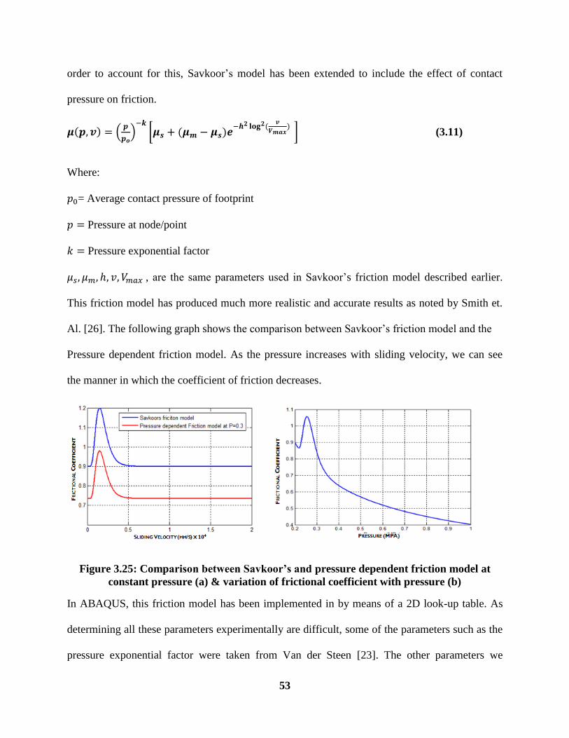
53
order to account for this, Savkoor’s model has been extended to include the effect of contact
pressure on friction.
𝝁(𝒑, 𝒗) = (𝒑
𝒑𝒐)
−𝒌
[𝝁𝒔 + (𝝁𝒎 − 𝝁𝒔)𝒆−𝒉𝟐 𝐥𝐨𝐠𝟐(
𝒗
𝑽𝒎𝒂𝒙)
] (3.11)
Where:
𝑝0= Average contact pressure of footprint
𝑝 = Pressure at node/point
𝑘 = Pressure exponential factor
𝜇𝑠, 𝜇𝑚, ℎ, 𝑣, 𝑉𝑚𝑎𝑥 , are the same parameters used in Savkoor’s friction model described earlier.
This friction model has produced much more realistic and accurate results as noted by Smith et.
Al. [26]. The following graph shows the comparison between Savkoor’s friction model and the
Pressure dependent friction model. As the pressure increases with sliding velocity, we can see
the manner in which the coefficient of friction decreases.
Figure 3.25: Comparison between Savkoor’s and pressure dependent friction model at
constant pressure (a) & variation of frictional coefficient with pressure (b)
In ABAQUS, this friction model has been implemented in by means of a 2D look-up table. As
determining all these parameters experimentally are difficult, some of the parameters such as the
pressure exponential factor were taken from Van der Steen [23]. The other parameters we

54
calculated based on the requirements for this thesis. With this model implemented, results at very
high slip angles could be achieved. It is very important to note that the implemented model just
provides an approximate prediction for the tire-road friction at the contact patch. In order to fully
understand and accurately predict the frictional coefficient, full-scale friction tests would need to
be performed in order to determine the frictional parameters used in equation 3.11. However, this
experimental determination is not within the scope of this thesis.

55
4.
TIRE-ROAD CONTACT
PRESSURE MEASUREMENT
4.1. Introduction
This chapter describes the experimental technique used to measure characteristics such as the
contact area and normal pressure distribution at the contact patch. The in-house experimental
procedure developed in order to obtain these characteristics is described in detail. The post-
processing methods and software used to accurately predict of the normal stress levels at the
contact patch are also described.
4.2. The Fujifilm Prescale pressure sensitive film
The Fujifilm Prescale film is a special type of pressure measuring film that allows the user to
visually see the variations in contact pressure levels and the contact area for a particular
application. This film is very useful for measuring contact pressure and is used multiple
industries which includes the aerospace, automotive, construction, electronic and the medical
industry. The film provides a high resolution distribution of the contact pressure levels; each
pixel is about 0.1mm x 0.1mm [27].
4.2.1. Fujifilm Prescale Pressure Sensitive Film Structure
The film structure consists of a “micro-encapsulated” color forming material and developing
material. There are two basic types of Prescale films:

56
i. Mono-sheet film type: This type of film is made from a polyester base on which a layer
of the color developing material is coated. The micro-encapsulated color-forming
material is layered over it. This type of film is generally used for higher contact
pressures. The pressure values range between 1250 PSI to 43000 PSI [27].
Figure 4.1: Mono-sheet Film Type structure [28]
"Prescale," Fujifilm, [Online]. Available:
http://www.fujifilm.com/products/prescale/prescalefilm/#See_All. [Accessed 08 30 2016].
Used under fair use 2016.
ii. Two-sheet film type: This type of film is composed of two polyester bases. One is
coated with a layer of micro-encapsulated color forming material (“A-film”) and the
other base is coated with a layer of the color-developing material (“C-Film”). The two
films each facing their respective coated sides would be sand-witched together. This type
of film is used for measuring lower pressure ranges of the order ranging from 29 PSI-
7250 PSI [27].
Figure 4.2: Two-sheet film type structure [28]
"Prescale," Fujifilm, [Online]. Available:
http://www.fujifilm.com/products/prescale/prescalefilm/#See_All. [Accessed 08 30 2016].
Used under fair use 2016.
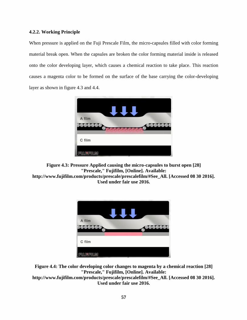
57
4.2.2. Working Principle
When pressure is applied on the Fuji Prescale Film, the micro-capsules filled with color forming
material break open. When the capsules are broken the color forming material inside is released
onto the color developing layer, which causes a chemical reaction to take place. This reaction
causes a magenta color to be formed on the surface of the base carrying the color-developing
layer as shown in figure 4.3 and 4.4.
Figure 4.3: Pressure Applied causing the micro-capsules to burst open [28]
"Prescale," Fujifilm, [Online]. Available:
http://www.fujifilm.com/products/prescale/prescalefilm/#See_All. [Accessed 08 30 2016].
Used under fair use 2016.
Figure 4.4: The color developing color changes to magenta by a chemical reaction [28]
"Prescale," Fujifilm, [Online]. Available:
http://www.fujifilm.com/products/prescale/prescalefilm/#See_All. [Accessed 08 30 2016].
Used under fair use 2016.

58
Using “Particle Size Control” technology, the micro-capsules are designed to react to various
degrees of pressures; releasing their color forming material at a density that corresponds to
specific levels of applied pressure. The size of micro-capsule and the strength of its wall have
correlation with pressure. Large micro-capsules are broken by low pressure and small micro-
capsules are broken by high pressure. Also, microcapsules with thin walls are broken by low
pressure and those with thick walls are broken by high pressure. Several tens of micro-capsules
in different sizes and wall strength are used in the Prescale film. Small micro-capsules are coated
on the Prescale to measure high pressure and large micro-capsules are coated on the Prescale to
measure low pressure. The volume of color forming material in micro-capsules and color
developing material decides the color density [29]. Figure 4.5 shows the color densities at
varying pressure levels.
Figure 4.5: Magenta Color densities at varying pressure levels [28]
"Prescale," Fujifilm, [Online]. Available:
http://www.fujifilm.com/products/prescale/prescalefilm/#See_All. [Accessed 08 30 2016].
Used under fair use 2016.
This technology also makes it possible to have films with different pressure operating ranges.
The different pressure ranges of the Fuji Prescale Films re-summarized in figure 4.6. For the
purpose of this thesis, the LLLW film type has been used which has an operating range of 0.2 to
0.8MPa.

59
Figure 4.6: Pressure Ranges for the Fuji-Film Prescale [27]
"Prescale," Fujifilm, [Online]. Available:
http://www.fujifilm.com/products/prescale/prescalefilm/#See_All. [Accessed 08 30 2016].
4.2.3. Conditions for applying pressure to Prescale Film
Extended Pressure measurement: With the extended pressure method, the applied pressure is
increasingly applied gradually up to the specified level and will be maintained continuously at
that level. In order to get the best and accurate results the pressure should be applied gradually up
to its highest value over a period of 2 minutes and it should be maintained at its highest level for
another couple of minutes [28].
Momentary Pressure Measurement: The Prescale film can also be used for momentary
pressure measurements. In this case the load should be applied gradually up to its highest
magnitude over a 5 second period, and should be maintained at the highest level for another 5
seconds. The momentary pressure measurement method has been adopted for this experimental
study as the contact pressures within the footprint vary between 0.4MPa to 0.8MPa [28].
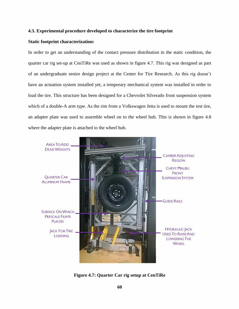
60
4.3. Experimental procedure developed to characterize the tire footprint
Static footprint characterization:
In order to get an understanding of the contact pressure distribution in the static condition, the
quarter car rig set-up at CenTiRe was used as shown in figure 4.7. This rig was designed as part
of an undergraduate senior design project at the Center for Tire Research. As this rig doesn’t
have an actuation system installed yet, a temporary mechanical system was installed in order to
load the tire. This structure has been designed for a Chevrolet Silverado front suspension system
which of a double-A arm type. As the rim from a Volkswagen Jetta is used to mount the test tire,
an adapter plate was used to assemble wheel on to the wheel hub. This is shown in figure 4.8
where the adapter plate is attached to the wheel hub.
Figure 4.7: Quarter Car rig setup at CenTiRe

61
Figure 4.8: Adapter plate mounted on wheel hub
The normal load is controlled manually by adding weights in the region shown in figure 4.7.
Three load cases were chosen for this experiment based on the maximum rated load for the tire
(load index). The maximum rated load for the tire is 615 kg. Load cases of 3400N, 4000N and
4800N were chosen, which corresponds to 55%, 67% and 80% of the rated load index. The rig
has guide rails on which the entire frame can move in the vertical direction. In order to raise and
lower the frame, a hydraulic jack is used. The suspension system is mounted on to the frame and
a provision has been included to adjust the camber for the wheel. The hydraulic frame lowers the
frame down such that the tire makes contact with the surface attached to the jack (shown in
yellow) in figure 4.7. Figure 4.9 shows the tire in contact with the Prescale©
film.
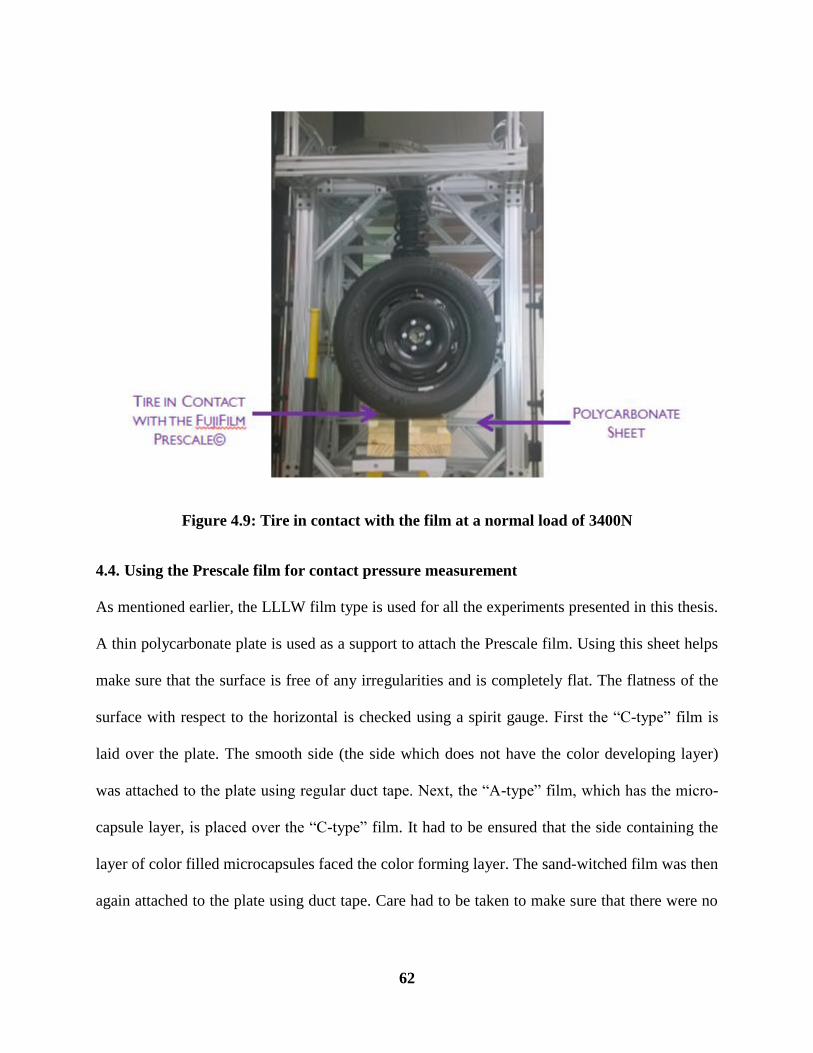
62
Figure 4.9: Tire in contact with the film at a normal load of 3400N
4.4. Using the Prescale film for contact pressure measurement
As mentioned earlier, the LLLW film type is used for all the experiments presented in this thesis.
A thin polycarbonate plate is used as a support to attach the Prescale film. Using this sheet helps
make sure that the surface is free of any irregularities and is completely flat. The flatness of the
surface with respect to the horizontal is checked using a spirit gauge. First the “C-type” film is
laid over the plate. The smooth side (the side which does not have the color developing layer)
was attached to the plate using regular duct tape. Next, the “A-type” film, which has the micro-
capsule layer, is placed over the “C-type” film. It had to be ensured that the side containing the
layer of color filled microcapsules faced the color forming layer. The sand-witched film was then
again attached to the plate using duct tape. Care had to be taken to make sure that there were no

63
air gaps between the two surfaces. The duct tape helped prevent any form of movement or
friction between the two polyester sheets.
4.4.1. Experimental Settings
It was very important to ensure that the camber was set to 00 in order to get a symmetric
footprint. This required a lot of fine tuning, adjustment and experimentation to make sure that
this was achieved.
4.4.2. Fujifilm Prescale Post-processing Techniques
Figure 4.10 shows the Prescale “C-film” (carrying the color developing layer), after a
momentary normal load of 3400N was applied at an inflation pressure of 35 PSI.
Figure 4.10: Fujifilm Prescale “C” film after application of load of 3400N at 35 PSI
4.4.3. Determining the normal pressure level using the Fujifilm Prescale
As discussed earlier, once the contact pressure is applied and released, the contact area would
have varying levels of magenta, depending on the pressure experienced in those regions. The

64
intensity of the color is directly proportional to the amount of pressure applied. The manual
process of determining the pressure level is described below:
i. The exposed “C-film” or the film carrying the color developing layer is compared against
the magenta color chart shown in figure 4.5. Each magenta sample corresponds to a
specific density so it is important to take note of it. As there would be instances where the
color lies in between the color intensities shown in figure 4.5, interpolation would need to
be followed.
ii. Using the graph of the temperature vs. humidity shown in figure 4.11, the nature of the
pressure values can be determined for the appropriate operating conditions. It is
important to note the temperature and humidity conditions accurately as these conditions
do significantly impact the contact pressure levels. Fujifilm recommends that the
operating temperature lies between 200 C to 300 C, and the humidity lies between 35%
RH – 80% RH. The accuracy of the contact pressure levels is about ±10%.
Figure 4.11: Graph of Humidity vs Temperature [28]
"Prescale," Fujifilm, [Online]. Available:
http://www.fujifilm.com/products/prescale/prescalefilm/#See_All. [Accessed 08 30 2016].
Used under fair use 2016.
iii. Once the appropriate area has been selected (A,B, C or D as shown in figure 4.11), using
the value of the density obtained in the previous step, it would be possible to determine

65
the contact pressure level, corresponding to the magenta color density as shown in the
graph in figure 4.12.
Figure 4.12: Graph of pressure vs density for momentary pressure measurements [28]
"Prescale," Fujifilm, [Online]. Available:
http://www.fujifilm.com/products/prescale/prescalefilm/#See_All. [Accessed 08 30 2016].
Used under fair use 2016.
4.5. Using the Topaq Pressure analysis system for post-processing:
Topaq is pressure analysis system that is developed by Sensor Products Inc. It consists of a
specially calibrated “densitimetric scanner” and a post-processing software. Using the Topaq
system, it is possible to achieve high resolution color calibrated images of the tire footprint. It
also can provide a wealth of statistical information about the footprint. This method easily
overcomes the difficulties of using the manual method to determine the pressure levels at the
contact patch. Results can be obtained easily and quickly. From left to right, Figure 4.13 (a)
shows the specially calibrated high resolution scanner and figure 4.13 (b) shows the laptop with
the Topaq software used for post processing the results. Figure 4.14 shows the analysis

66
capabilities of the software. Figure 4.15 shows the post-processed contact pressure distribution
across the contact patch using the Topaq pressure analysis system.
Figure 4.13: Topaq system: Specially calibrated Scanner (a) and software system (b)
Figure 4.14: Topaq Software capabilities

67
Figure 4.15: Post-processed normal pressure distribution across the contact patch
4.6. Important Precautions to be taken while using the Prescale film
The film reacts with high sensitivity to every second of pressure applied. The two films were to
be bound together at the ends using duct tape, to prevent any form of relative motion between the
A-film and the C-film. Fujifilm recommends that the operating temperature lies between 200C to
350C, and the relative humidity lies between 35% RH to 80% RH. The film is very delicate and
care has to be taken not to touch the coated side of A-film, when sand-witched with the C-film as
the color filled microcapsules can be broken with a very small application of pressure.

68
5.
FINITE ELEMENT MODEL
VALIDATION
5.1. Introduction
In this chapter, the developed finite element model is validated against the experimental footprint
results obtained from the in-house experimental procedure discussed in Chapter 4. First, a brief
overview of general footprint physics along with the standard conventions followed is discussed.
Next, footprint results and studies are presented. The experimental footprint results are compared
with the simulation results in the static condition and at slow rolling speeds. The effects of
changes in normal load and inflation pressure on the footprint shape and contact pressure
distribution are studied in detail. Possible reasons for the differences in results are also discussed.
The effects of cornering and an inclination angle on the footprint phenomena are also presented.
5.2. General Footprint Physics
The footprint is a kinematically driven boundary. Contact between the tire and road leads to a
complex distribution of stresses across the interface. At each point within the footprint, there
exists a normal component and two shear components. The precise nature of the stress
distribution field depends on the forces and kinematic conditions existing at a given instant, the
tire’s structure, and frictional coefficient between the tire and the road [9].
As mentioned in chapter 2, the tire is a doubly-curved object. It is curved in the circumferential
direction as well as the transverse direction. This attribute causes the tire structure to bend,
stretch compress in order to conform to the road surface. There are many factors that contribute
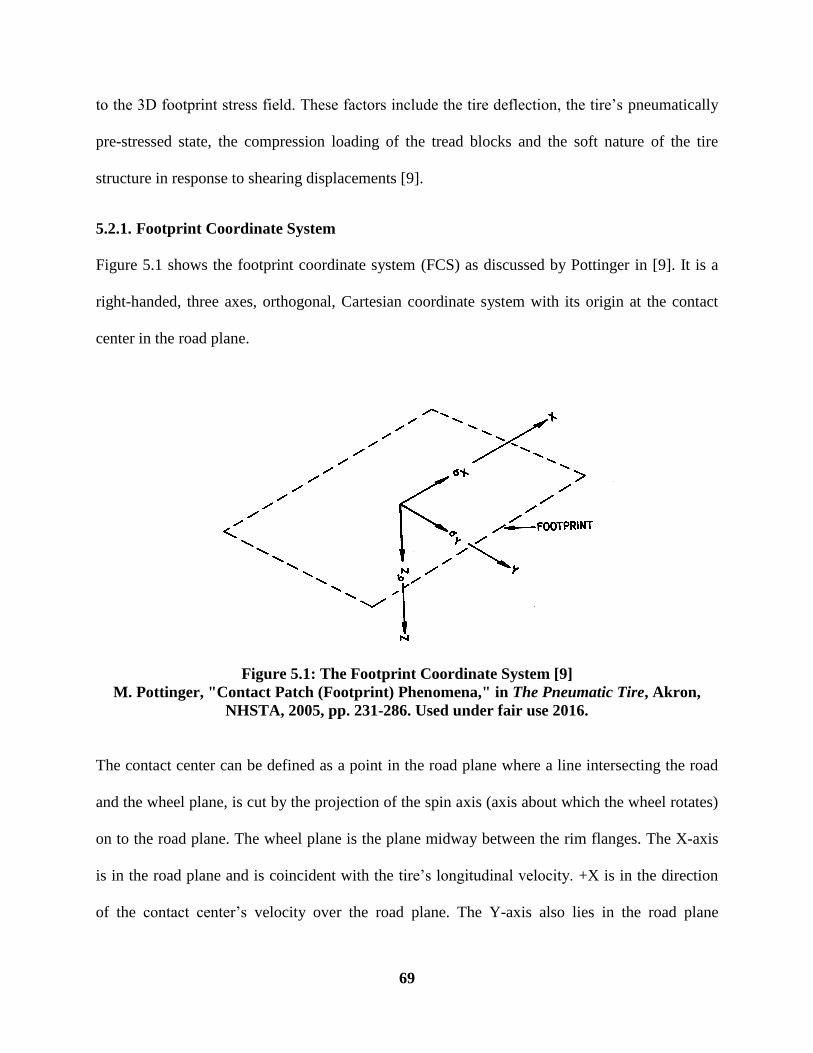
69
to the 3D footprint stress field. These factors include the tire deflection, the tire’s pneumatically
pre-stressed state, the compression loading of the tread blocks and the soft nature of the tire
structure in response to shearing displacements [9].
5.2.1. Footprint Coordinate System
Figure 5.1 shows the footprint coordinate system (FCS) as discussed by Pottinger in [9]. It is a
right-handed, three axes, orthogonal, Cartesian coordinate system with its origin at the contact
center in the road plane.
Figure 5.1: The Footprint Coordinate System [9]
M. Pottinger, "Contact Patch (Footprint) Phenomena," in The Pneumatic Tire, Akron,
NHSTA, 2005, pp. 231-286. Used under fair use 2016.
The contact center can be defined as a point in the road plane where a line intersecting the road
and the wheel plane, is cut by the projection of the spin axis (axis about which the wheel rotates)
on to the road plane. The wheel plane is the plane midway between the rim flanges. The X-axis
is in the road plane and is coincident with the tire’s longitudinal velocity. +X is in the direction
of the contact center’s velocity over the road plane. The Y-axis also lies in the road plane

70
perpendicular to the X-axis. +Y is to the right when the system is viewed from the rear looking
in the positive X-direction. The Z-axis is defined by the cross product of +X into +Y. It is
perpendicular to the road plane with its positive sense into the road plane as discussed by
Pottinger in [9].
5.2.2. Footprint Stress Definition
Figure 5.2: Footprint Stress Definition [9]
M. Pottinger, "Contact Patch (Footprint) Phenomena," in The Pneumatic Tire, Akron,
NHSTA, 2005, pp. 231-286. Used under fair use 2016.
As mentioned in section 5.2 at every point within the footprint, there exists two shear stress
components and one normal stress component. The shear stress in the X-direction is referred to
as the longitudinal shear stress 𝜎𝑥, and the shear stress in the Y direction is referred to as the
lateral shear stress 𝜎𝑦. The normal stress represented by 𝜎𝑧. Positive longitudinal stress +𝜎𝑥
pushes the tire forward and negative longitudinal stress −𝜎𝑥 causes the tire to decelerate.
Positive lateral stress +𝜎𝑦 pushes the tire to the right and the negative lateral stress −𝜎𝑦 pushes
the tire to the left. The normal stress 𝜎𝑧 generated at the contact gives an indication of the load
applied on the tire.

71
5.2.3. Footprint Position Definitions
The Figures 5.3 and 5.4 show the direction of the rolling tire and the resulting footprint image as
the tire rolls. The edge of the footprint with the most positive X-value is referred to as the
footprint leading edge. The edge with the most negative X-value is referred to as the footprint
trailing edge. For tread blocks, the first edge to enter contact with the road (block leading edge)
is referred to as the heel. The last edge to enter contact, the block trailing edge, is referred to as
the toe. Ribs are counted from left to right along the Y-axis in order of increasing Y.
Figure 5.3: Top View Direction of Rolling Tire
Figure 5.4: Resulting Footprint Image

72
5.3. Static Footprint Results
In the following sections the experimental footprint results obtained from the procedure
described in chapter 3 are compared with the finite element simulation results. Studies are done
at three different inflation pressures: 35PSI, 30PSI and 40PSI, in order to study the effect of
changes in inflation pressure on the footprint characteristics. Studies are also conducted with
three different normal load cases: 3400N, 4000N and 4800N in order to understand the effect of
the changes in normal load on the contact pressure distribution and footprint shape. These
normal load cases are chosen based on the maximum rated load index for the tire which is 615
Kg. Note that all the stress results are expressed in terms of MPa and the length units are
expressed in mm throughout this chapter. Note that above each footprint image the footprint
length and width have been indicated in mm.
5.3.1. Footprint results and studies at 35PSI
5.3.1.1. Case 1: Normal Load of 3400N
Footprint Length: 95mm, Footprint Width: 137mm
Figure 5.5: Experimental Footprint at 35 PSI, 3400N

73
From figure 5.5 we can see that the highest contact pressure zones occur relatively around the
shoulders of the tire. The center region has relatively lower contact pressures in comparison with
the shoulders. This is quite characteristic of a passenger car tire as discussed by Pottinger in [9]
Footprint Length: 97mm, Footprint Width: 141mm
Figure 5.6: FE Simulation Footprint at 35 PSI, 3400N
On comparing figures 5.5 and 5.6 we can see that the footprint shape and the peak stress levels at
the contact patch in both cases are quite comparable. However it’s quite evident from figures that
the distribution of stresses across the contact patch is not exactly the same in both cases. There
could be a number of reasons as for these differences. They are outlined below:
i. Inaccurate material characterization: As mentioned in chapter 3, hardness tests were
used to characterize the elastic properties of the rubber compounds. Although this
technique gives a reasonable estimate of the actual values, it may not provide very
accurate results. DMA testing would need to be done on green samples of each of the tire
compounds to characterize the material properties more accurately. The properties of the
apex (chaffer), sidewall, and beads significantly affect the sidewall stiffness which in turn
has a very significant impact on the pressure distribution at the contact patch. The elastic

74
properties for the belts, carcass plies and nylon cap plies have been taken from the results
published by Balaramakrishna et. Al. in [18]. However, these values could be
significantly different from the actual elastic properties of the cords used in the test tire.
These differences could result in different a pneumatic pre-stressed state, which
eventually causes different effects due to the relaxation of the loads on the belt cords
around the center of the contact region [9].
Figure 5.7: Relaxation of the cord loads under a static load of 3400N
It’s evident from that the simulation results that belt cords seem to have a higher amount
of “relaxation” going on at center of the contact patch compared to the actual case as seen
in figure 5.7.
ii. Inaccurate geometric representation: As mentioned earlier, having an accurate
representation of the geometric details of the tire is extremely important in the tire
modeling process. Small differences in profile geometries could result in vastly different
footprint shapes and contact pressure distribution patterns. Although an immense amount
of care has been taken to represent the geometry as closely as possible to the
experimental case, it still may not be a very accurate representation of the actual tire. The

75
2D geometric model would need to be compared with the actual layout of the tire to see if
there are any significant differences.
iii. Boundary conditions and friction: As mentioned earlier in chapter 3, the tire essentially
has 3 contact regions: a contact zone between the tire and road, and two contact regions
between the rim and bead regions. This finite element model does not include a rim,
which implies that the rim-strip region nodes (the region around the beads which is in
contact with the rim) are fixed in position. There is no friction value given between these
two surfaces. This again could affect the overall stiffness of the tire and thus affect the
contact pressure distribution pattern. The friction between the surface and the tread could
be another possible reason. In the experimental test, the tire is brought in contact with the
Prescale film. The coefficient of friction between these two surfaces has not been
determined experimentally. However given the smooth nature of the film, a low value of
the coefficient of friction could be expected. The finite element model uses a coefficient
of friction of zero between the tire and the surface in order to avoid convergence issues,
in the static condition. This could again affect the contact pressure distribution results.
iv. Differences in tread geometry features: This could be another potential cause for the
differences. As seen in figure 5.5, sipes are present on the tread pattern. This would result
in a significantly different tread stiffness compared to the stiffness without the presence
of sipes. Generally, the presence would decrease the tread modulus and could have an
impact on the distribution of the measured contact stresses. The tread pattern modeled in
ABAQUS does not account for the presence of sipes, as this would cause difficulties in
meshing the tread pattern.

76
Figure 5.8: Average contact stress distribution across the center rib at 35PSI, 3400N
Figure 5.8 shows a comparison between the average contact pressure distribution across the
center rib, for simulation and experimental results. Note that the average values across the entire
rib were compared in both cases. As seen from the figure, the contact pressure results are
reasonably comparable, however higher stresses are observed in the case of the experimental
result as mentioned earlier.
5.3.1.2. Case 2: Normal Load of 4000N
From figures 5.9 and 5.10 we can see that increasing the normal load, has increased the footprint
length and width significantly. The percentage increase in overall contact area was found to be
around 23%, as a result of increasing the load by 18%.

77
Footprint Length: 107mm, Footprint Width: 148mm
Figure 5.9: Experimental Footprint at 35 PSI, 4000N
Footprint Length: 110mm, Footprint Width: 152mm
Figure 5.10: Simulation Footprint at 35 PSI, 4000N
The footprint shape and size seem to be reasonably comparable to each other. The peak values of
the stresses in both cases are comparable as well. Again, as noted earlier, in the case of the
experimental results higher stresses are found around the center of the patch compared to the
simulation footprint results.

78
Figure 5.11: Average pressure distribution across the center rib at 35PSI, 4000N
Figure 5.11 shows the comparison between the average contact pressure distributions in both
cases. The results again seem to be reasonably comparable to each other, however higher stress
levels are observed in the case of the experimental result. Another point to note from looking at
the graph is that the average contact pressure distribution across the rib, in the experiment case,
is not exactly symmetrical in nature. This can be attributed due to the experimental conditions
while conducting the experiment. A very slight movement of the surface of the jack was
observed under the application of the load. This could be a reason for the non-symmetrical
contact pressure distribution.
5.3.1.3. Case 3: Normal Load of 4800N
We can again see that by increasing the normal load, the footprint length width and area have
increased significantly. By increasing the normal load by 20%, results in an increase in contact
area by 22%. The results for the overall dimensions and peak stress values are very comparable
between the finite element and experimental results.

79
Footprint Length: 112mm, Footprint Width: 151mm
Figure 5.12: Experimental Footprint at 35 PSI, 4800N
Footprint Length: 115mm, Footprint Width: 153mm
Figure 5.13: FE Simulation Footprint at 35 PSI, 4800N
Figure 5.14: Average pressure distribution across the center rib at 35PSI, 4800N

80
5.3.1.4. Footprint results summary at 35PSI
Table 5.1 gives a comparative summary of all the results related to the contact patch dimensions
at 35PSI. Table 5.2 shows the result summary for the footprint area and the actual load
(calculated) summary acting at the contact patch at the same inflation pressure. The actual load is
calculated by integrating the pressure across the entire area of the contact patch.
Load (N) Experiment FE Simulation Error
Contact Patch Length (mm)
3400 95 97 0.97%
4000 105 110 3.48%
4800 112 115 2.34%
Contact Patch Width (mm)
3400 137 141 0.71%
4000 148 152 0.00%
4800 151 153 1.31%
Table 5.1: Static footprint overall dimensions summary at 35 PSI at varying normal loads
Load (N) Experiment Contact Area
(mm2)
FE Simulation Contact
Area (mm2)
Error Actual Load
(N)
3400 6665 7057 5.88% 3382.3
4000 8075 8656 7.20% 3947.1
4800 9738 10463 7.45% 4772.5
Table 5.2: Static footprint area & actual load summary at 35 PSI at varying normal loads
5.3.2. Footprint results and studies at 30 PSI
5.3.2.1. Case 1: Normal Load of 3400N
Comparing this result shown in figure 5.15 with the same load case at 35 PSI shown in figure 5.5
we can firstly see that this has resulted in an increased footprint area by around 15%. Another
important point to note is that the distribution of stresses around the center is comparatively
lower compared to the same load case a 35 PSI. Lowering the inflation pressure would imply
that the tire’s pre-tensioned state changes. As discussed earlier, the tire is doubly-curved in
nature; a curvature exists in the circumferential direction as well as in the lateral direction.
Decreasing the inflation pressure would result in a change in the overall shape of the tire due to

81
the change in the tire’s pre-tensioned state. This implies that the overall stiffness of the tire
changes. The loaded radius for the tire would now decrease as a result of the increased deflection
and reduced sidewall stiffness.
Footprint Length: 103mm, Footprint Width: 140mm
Figure 5.15: Experimental Footprint at 30 PSI, 3400N
Footprint Length: 103mm, Footprint Width: 140mm
Figure 5.16: Simulation Footprint at 30 PSI, 3400N
On comparing figure 5.16 with figure 5.15 we can again see that the footprint length, with and
area results between the simulation and the experimental case are quite comparable. Comparing

82
this simulation result with the same simulation case at 35 PSI, shown in figure 5.6, we can see
that the contact area has increased, but at the same time the contact stresses are slightly lower,
which is typically expected as discussed in [30]. Figure 5.17 compares the average pressure
distribution across the center rib of the contact patch at 30PSI and 3400N between the simulation
and the experimental results.
Figure 5.17: Average pressure distribution across the center rib at 30PSI, 3400N
5.3.2.2. Case 2: Normal Load of 4000N
Footprint Length: 115mm, Footprint Width: 150mm
Figure 5.18: Experimental Footprint at 30 PSI, 4000N

83
On comparing the result shown figure 5.18 with experimental case shown in figure 5.15 (3400N
load case), we can again see that increasing the normal load by 18% has significantly increased
the contact patch area by about 22%. As discussed earlier, there are significantly lower stress
values around the center of the contact patch, in comparison with the load case at 4000N. Figure
5.19 shows the simulation footprint.
Footprint Length: 119mm, Footprint Width: 150mm
Figure 5.19: Simulation Footprint at 30 PSI, 4000N
Figure 5.20: Average pressure distribution across the center rib at 30PSI, 4000N
Figure 5.20 shows how the average pressure distribution across the center rib of the contact patch
at 30PSI and 4000N between the simulation and the experimental results varies.
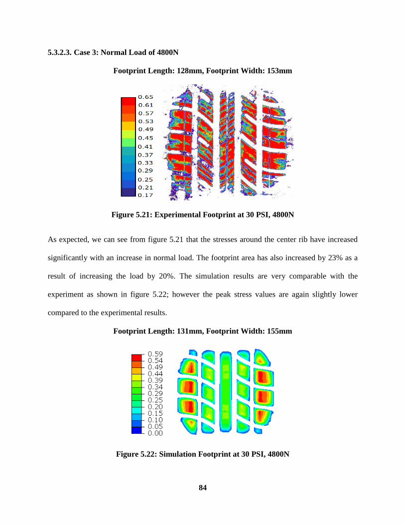
84
5.3.2.3. Case 3: Normal Load of 4800N
Footprint Length: 128mm, Footprint Width: 153mm
Figure 5.21: Experimental Footprint at 30 PSI, 4800N
As expected, we can see from figure 5.21 that the stresses around the center rib have increased
significantly with an increase in normal load. The footprint area has also increased by 23% as a
result of increasing the load by 20%. The simulation results are very comparable with the
experiment as shown in figure 5.22; however the peak stress values are again slightly lower
compared to the experimental results.
Footprint Length: 131mm, Footprint Width: 155mm
Figure 5.22: Simulation Footprint at 30 PSI, 4800N
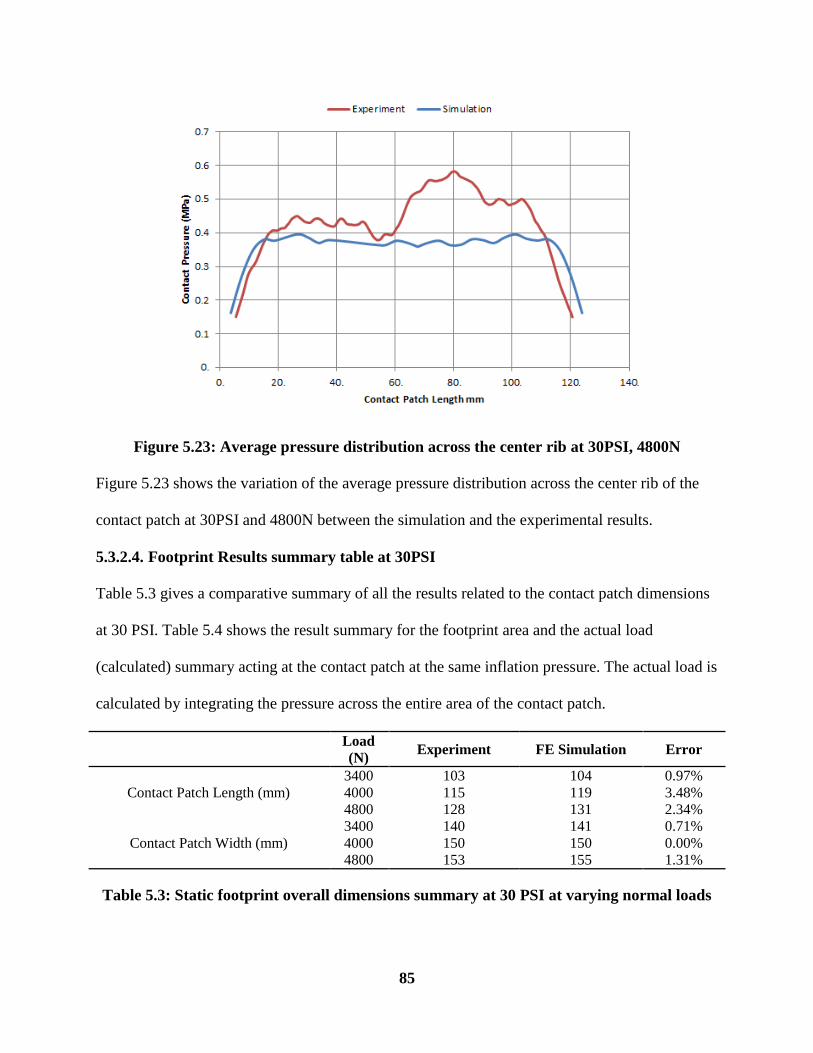
85
Figure 5.23: Average pressure distribution across the center rib at 30PSI, 4800N
Figure 5.23 shows the variation of the average pressure distribution across the center rib of the
contact patch at 30PSI and 4800N between the simulation and the experimental results.
5.3.2.4. Footprint Results summary table at 30PSI
Table 5.3 gives a comparative summary of all the results related to the contact patch dimensions
at 30 PSI. Table 5.4 shows the result summary for the footprint area and the actual load
(calculated) summary acting at the contact patch at the same inflation pressure. The actual load is
calculated by integrating the pressure across the entire area of the contact patch.
Load
(N) Experiment FE Simulation Error
Contact Patch Length (mm)
3400 103 104 0.97%
4000 115 119 3.48%
4800 128 131 2.34%
Contact Patch Width (mm)
3400 140 141 0.71%
4000 150 150 0.00%
4800 153 155 1.31%
Table 5.3: Static footprint overall dimensions summary at 30 PSI at varying normal loads
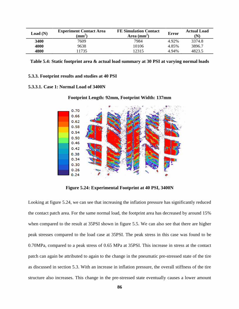
86
Load (N) Experiment Contact Area
(mm2)
FE Simulation Contact
Area (mm2)
Error Actual Load
(N)
3400 7609 7984 4.92% 3374.8
4000 9638 10106 4.85% 3896.7
4800 11735 12315 4.94% 4823.5
Table 5.4: Static footprint area & actual load summary at 30 PSI at varying normal loads
5.3.3. Footprint results and studies at 40 PSI
5.3.3.1. Case 1: Normal Load of 3400N
Footprint Length: 92mm, Footprint Width: 137mm
Figure 5.24: Experimental Footprint at 40 PSI, 3400N
Looking at figure 5.24, we can see that increasing the inflation pressure has significantly reduced
the contact patch area. For the same normal load, the footprint area has decreased by around 15%
when compared to the result at 35PSI shown in figure 5.5. We can also see that there are higher
peak stresses compared to the load case at 35PSI. The peak stress in this case was found to be
0.70MPa, compared to a peak stress of 0.65 MPa at 35PSI. This increase in stress at the contact
patch can again be attributed to again to the change in the pneumatic pre-stressed state of the tire
as discussed in section 5.3. With an increase in inflation pressure, the overall stiffness of the tire
structure also increases. This change in the pre-stressed state eventually causes a lower amount

87
of “relaxation” of the loads on the belt cords around the crown region. As a result, the contact
stresses have increased.
Footprint Length: 97mm, Footprint Width: 142mm
Figure 5.25: Simulation Footprint at 40 PSI, 3400N
Comparing the experimental and simulation results shown in figures 5.24 and 5.25 we can see
that the highest/peak stresses, footprint length, width and contact area are very similar. However,
the distribution of stresses around the crown region of the footprint is different on comparison
with each other. Figure 5.26 shows how the average pressure distribution across the center rib of
the contact patch at 40PSI and 3400N between the simulation and the experimental results
varies. Possible reasons for these differences in the distribution of stresses are cited in section
5.3.

88
Figure 5.26: Average pressure distribution across the center rib at 40PSI, 3400N
5.3.3.2. Case 2: Normal Load of 4000N
Footprint Length: 97mm, Footprint Width: 144mm
Figure 5.27: Experimental Footprint at 40 PSI, 4000N
Looking at figure 5.27, we can see that the footprint area has increased as expected. However the
percentage change obtained as a result of increasing the load by 18% is lower on comparison
with the percentage changes obtained at 35PSI and 30PSI for the same increase in normal load.
The percentage increase in footprint area in this case was found to be 12% compared to the

89
percentage increases of 23% and 22% at 35PSI and 30PSI respectively. This shows the highly
non-linear and complex nature of the tire. Comparing figures 5.27 and 5.28 we can see that the
peak stresses, footprint shape and size of the contact patch are very comparable. Figure 5.29
shows the variation of the average pressure distribution across the center rib of the contact patch
at 40PSI and 4000N between the simulation and the experimental results.
Footprint Length: 102mm, Footprint Width: 149mm
Figure 5.28: Simulation Footprint at 40 PSI, 4000N
Figure 5.29: Average pressure distribution across the center rib at 40PSI, 4000N

90
5.3.3.3. Case 3: Normal Load of 4800N
Footprint Length: 113mm, Footprint Width: 151mm
Figure 5.30: Experimental Footprint at 40 PSI, 4800N
Increasing the normal load further has increased the length and the footprint area. However the
increase in contact area is again not as prominent as the percentage increases in case of the 35PSI
and 30PSI test cases. The percentage increase in area was found to be around 13% by increasing
the load by 20%. The footprint shape, size and peak stress distribution at the contact patch are
very comparable comparing figures 5.30 and 5.31.
Footprint Length: 116mm, Footprint Width: 155mm
Figure 5.31: Simulation Footprint at 40 PSI, 4800N
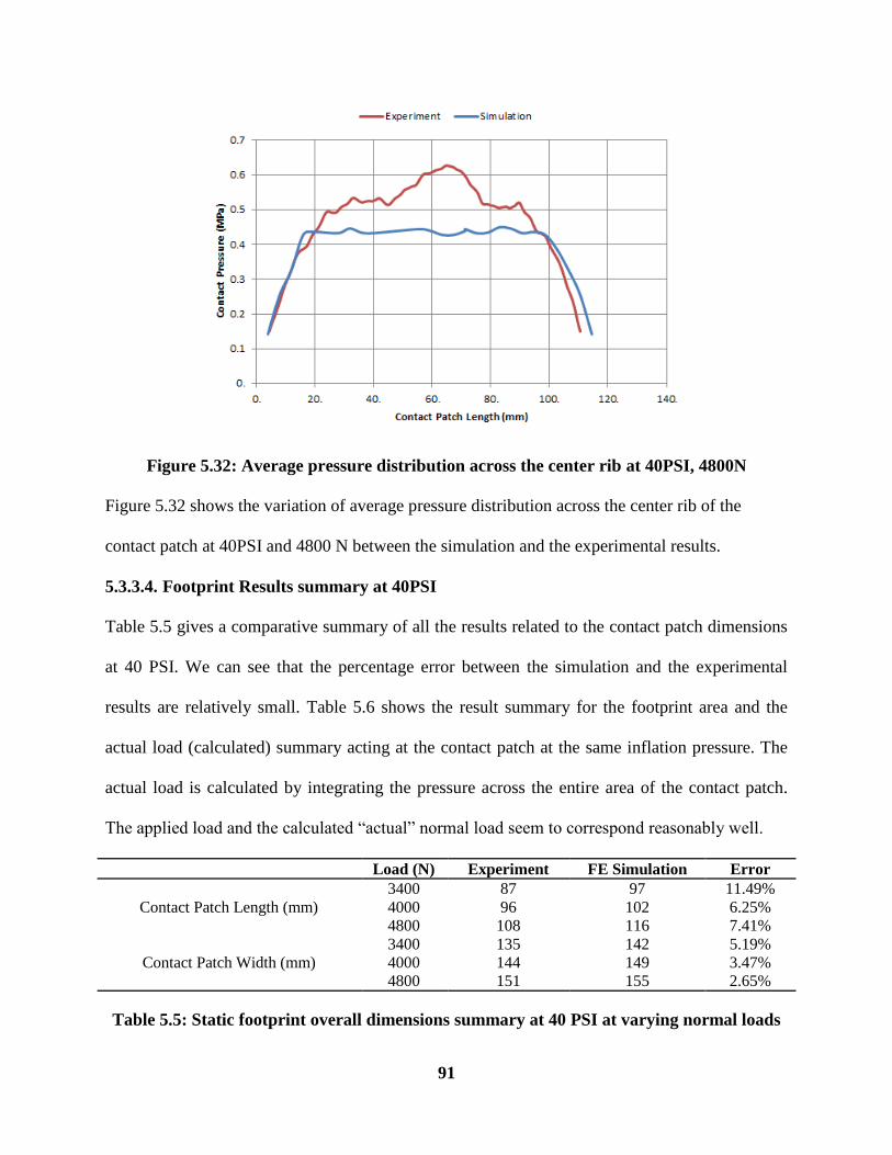
91
Figure 5.32: Average pressure distribution across the center rib at 40PSI, 4800N
Figure 5.32 shows the variation of average pressure distribution across the center rib of the
contact patch at 40PSI and 4800 N between the simulation and the experimental results.
5.3.3.4. Footprint Results summary at 40PSI
Table 5.5 gives a comparative summary of all the results related to the contact patch dimensions
at 40 PSI. We can see that the percentage error between the simulation and the experimental
results are relatively small. Table 5.6 shows the result summary for the footprint area and the
actual load (calculated) summary acting at the contact patch at the same inflation pressure. The
actual load is calculated by integrating the pressure across the entire area of the contact patch.
The applied load and the calculated “actual” normal load seem to correspond reasonably well.
Load (N) Experiment FE Simulation Error
Contact Patch Length (mm)
3400 87 97 11.49%
4000 96 102 6.25%
4800 108 116 7.41%
Contact Patch Width (mm)
3400 135 142 5.19%
4000 144 149 3.47%
4800 151 155 2.65%
Table 5.5: Static footprint overall dimensions summary at 40 PSI at varying normal loads

92
Load (N) Experiment Contact Area
(mm2)
FE Simulation Contact
Area (mm2)
Error Actual Load
(N)
3400 5799 6029 3.97% 3374.8
4000 6494 6768 4.21% 3896.7
4800 7339 7670 4.52% 4823.5
Table 5.6: Static footprint area & actual load summary at 40 PSI at varying normal loads
5.4. Slow rolling footprint studies
Although the static footprint gives us very useful information is it very important to understand
the changes in the distribution of stresses, when the condition is changed from static to a
dynamic condition. Slow rolling footprint studies were done using the lab’s Volkswagen Jetta as
shown in figure 5.33. Two tests were conducted in order to understand the difference in contact
pressure distribution due to changes in normal load in the dynamic state. For this purpose, one
test was done considering the load on the front-left tire and the other test was done considering
the load at the rear-right tire. The normal load on the front-left tire was found to be 4200N and
the normal load on the rear-right tire was found to be 3100N. In this section, the experimental
slow-rolling footprints are first compared with the static experimental results to get an
understanding and reasons for the changes in stress distribution from static to slow-rolling. It is
also important to note that a constant Coulomb’s friction model has been implemented in this
case as the speed is extremely low. These tests are performed at a speed of 2mph. A constant
friction of 0.8 was used. The simulation steady state results are then compared with the
experimental results. The reasons for the possible differences are noted and discussed.

93
Figure 5.33: Slow-rolling footprint test using the Jetta at approx. 2mph
5.4.1. Footprint at 4200N, 35PSI (Front-Left Tire of Jetta)
Figure 5.34: Experimental Slow-Rolling Footprint at 35 PSI, 4200N
Looking at figure 5.34 we can see that the result in the case of slow rolling is vastly different
from the result in the experimental case in the static condition. On comparison with the static

94
case, at the same normal load and inflation conditions, the peak normal stress levels increased
from 0.65MPa to 0.75MPa from the static to the dynamic condition respectively. The stresses
around the center of the contact patch have reduced significantly as well. From the figure we can
see that the average pressure distribution across the center rib of the contact patch is about 0.4
MPa, which is lower compared to the static case in figure 5.9. As noted by Pottinger [9], the
shoulder normal stress should significantly increase and the crown region normal stress would
decrease significantly when the condition changes from static to slow-rolling as shown in figure
5.35. The change in the normal stress pattern is associated with the change in the lateral stress
from static to rolling as shown in figure 5.36. Here, the outward directed lateral stresses are
grossly reduced in the rolling condition. The motion occurring in rolling frees the shoulders to
move in under the influence of the relaxation of belt cord tension in the footprint. Relatively, the
shoulders move in and roll under while the center region tends to deform further from the road
reducing the crown normal stress magnitude.
Figure 5.35: Changes in normal stress distribution from the static to slow-rolling [9]
M. Pottinger, "Contact Patch (Footprint) Phenomena," in The Pneumatic Tire, Akron,
NHSTA, 2005, pp. 231-286. Used under fair use 2016.

95
Figure 5.36: Changes in lateral stress distribution from the static to slow-rolling [9]
M. Pottinger, "Contact Patch (Footprint) Phenomena," in The Pneumatic Tire, Akron,
NHSTA, 2005, pp. 231-286. Used under fair use 2016.
Figure 5.37: Changes in lateral and normal stresses from static to rolling
M. Pottinger, "Contact Patch (Footprint) Phenomena," in The Pneumatic Tire, Akron,
NHSTA, 2005, pp. 231-286. Used under fair use 2016.
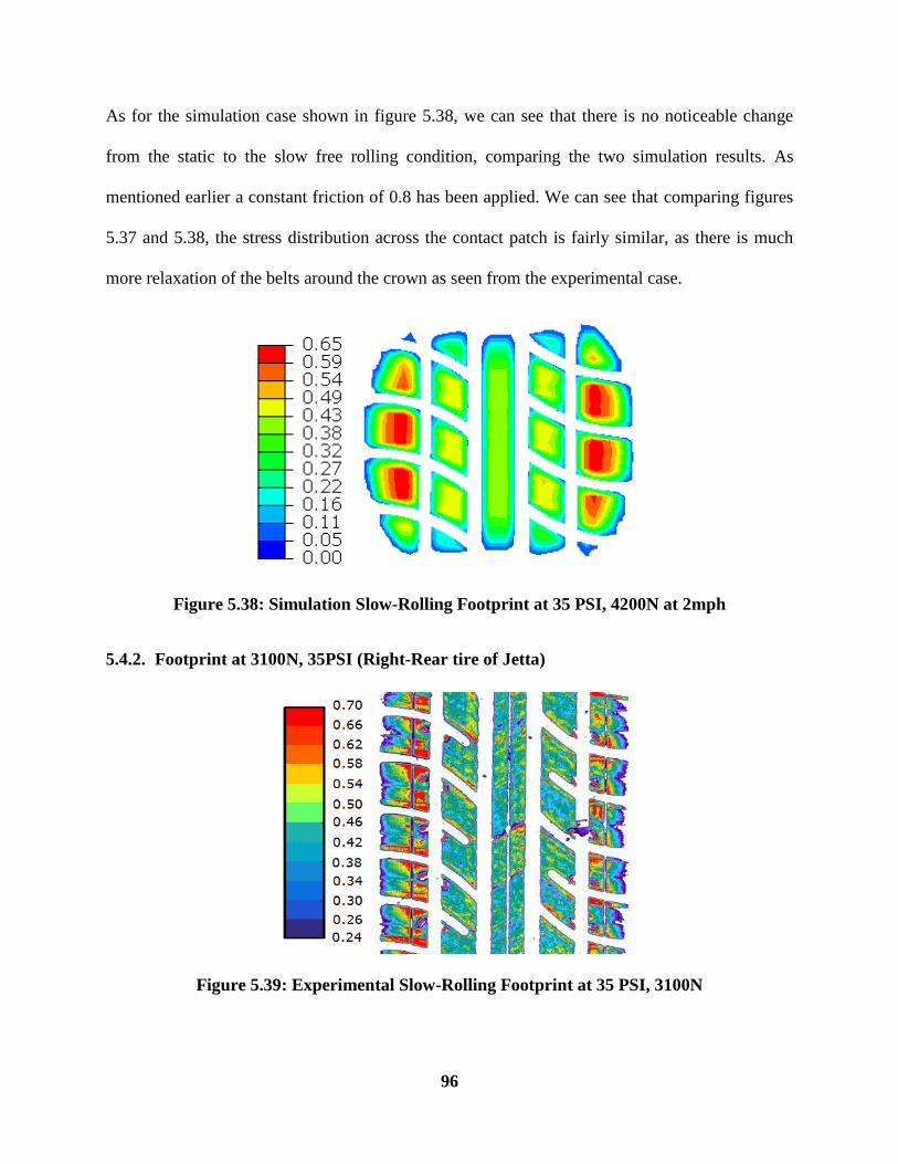
96
As for the simulation case shown in figure 5.38, we can see that there is no noticeable change
from the static to the slow free rolling condition, comparing the two simulation results. As
mentioned earlier a constant friction of 0.8 has been applied. We can see that comparing figures
5.37 and 5.38, the stress distribution across the contact patch is fairly similar, as there is much
more relaxation of the belts around the crown as seen from the experimental case.
Figure 5.38: Simulation Slow-Rolling Footprint at 35 PSI, 4200N at 2mph
5.4.2. Footprint at 3100N, 35PSI (Right-Rear tire of Jetta)
Figure 5.39: Experimental Slow-Rolling Footprint at 35 PSI, 3100N

97
In figure 5.39, we can firstly see the very significant effect of an inclination angle on the
footprint. The camber angle is about −1.450 which is the stock setting on the Jetta. Due to a
small amount of negative camber, higher stresses around the left shoulder are visibly noticeable
in comparison with the right shoulder. The area contact on the left shoulder is much greater
compared to the right.
Comparing this experimental result with the static experimental case at 3400N (shown in figure
5.5) we can again see that the shoulder normal stress levels are significantly higher than the
stress levels in the static case. The crown region normal stress levels have dropped as well. The
reasons for these differences are noted in section 5.4.1. Comparing figures 5.39 and 5.40 we can
see that the contact pressure distribution and the peak pressure levels are very similar as
mentioned earlier. This is primarily due to the amount of relaxation going on in the belts the
dynamic case compared to the static case.
Figure 5.40: Simulation Slow-Rolling Footprint at 35 PSI, 3100N
5.5. 3D Steady –State free rolling footprint stress analysis
One of main objectives of this thesis is to explore to the capabilities of this finite element model
as getting experimental results for the lateral and longitudinal stresses are quite difficult and

98
expensive. As this developed finite element tire model can give a reasonable prediction of the
footprint shape and pressure distribution at the contact patch, we will now take a closer look at
the footprint 3D stress field in the steady state free rolling condition. It is very important to note
that the pressure dependent friction model described in chapter 3 has been activated in these
simulations. Coulomb’s friction model at such high speeds results in excessive distorted
elements around the tread and does not yield accurate results.
5.5.1. Normal Stress Distribution:
These simulation results are presented at a speed of 40mph, an inflation pressure of 35PSI and a
normal load of 4800N, with the pressure dependent friction model activated. Figure 5.42 shows
the normal stress distribution across the contact patch as described by Pottinger [9].
Figure 5.41: Normal Pressure Distribution at 35PSI, 4800N and 40mph
Generally passenger tires typically show the largest normal stress levels on the shoulders and
lower normal stress levels around the crown region as discussed by Pottinger in [9]. From the
simulation results shown in figure 5.41, we can see that the tire model exhibits similar
characteristics.

99
Figure 5.42: Normal stress distribution for a general passenger tire [9]
M. Pottinger, "Contact Patch (Footprint) Phenomena," in The Pneumatic Tire, Akron,
NHSTA, 2005, pp. 231-286. Used under fair use 2016.
5.5.2. Longitudinal stress distribution
Figure 5.43 shows the longitudinal stress distribution across the contact patch. As seen from the
figure, the leading edge of the footprint has more positive stresses (shown in red) in comparison
with the trailing edge of the footprint which has more negative stresses (shown in blue). We can
also see that the longitudinal stresses around the shoulders are more positive in comparison with
the crown region stresses. The reason behind this phenomenon is due to the fact that different
parts of the tire (laterally across the tread) have different effective radii which cause one part to
go further than the other within a tire revolution. The shoulders essentially have a larger effective
rolling radius than the crown, which accounts for the difference in stress levels as shown in
figure 5.44 described by Pottinger [9].

100
Figure 5.43: Longitudinal stress distribution
Figure 5.44: Longitudinal stress distribution for a general passenger tire [9]
M. Pottinger, "Contact Patch (Footprint) Phenomena," in The Pneumatic Tire, Akron,
NHSTA, 2005, pp. 231-286. Used under fair use 2016.
5.5.3. Lateral stress distribution
Figure 5.45 shows the lateral stress distribution pattern across the contact patch. The lateral
stresses also show the effect of cord load relaxation as mentioned earlier in section 5.4. Here the
right shoulder shows carries positive stresses compared to the left shoulder which carries more

101
negative stresses. This is again typically expected for a passenger tire as discussed by Pottinger
[9] as shown in figure 5.46.
Figure 5.45: Lateral stress distribution at 4800N, 35PSI and 40mph
Figure 5.46: Longitudinal stress distribution for a general passenger tire [9]
M. Pottinger, "Contact Patch (Footprint) Phenomena," in The Pneumatic Tire, Akron,
NHSTA, 2005, pp. 231-286. Used under fair use 2016.
5.6. Effect on cornering on the 3D-Stress distribution
This next section discusses the 3D stress distribution field when a cornering maneuver is
negotiated. The same test case conditions as used in the previous section are used. The normal
load applied to the tire is 4800N, the inflation pressure is 35PSI and the longitudinal velocity is

102
40mph. A slip angle case of −30 is presented. The pressure dependent friction model has been
activated again as Coulomb’s friction model does not yield satisfactory results.
5.6.1. Normal stress distribution
The presence of a slip angle reshapes the footprint into a rough trapezoid in the road plane [10].
A left turn leads to a long right shoulder and a short left shoulder. As evident from figure 5.47, a
right turn is being negotiated, which causes a longer shoulder on the left most rib of the tire. It
also has been observed that increasing the slip angle results in an increase in peak normal stress
around the shoulder carrying the greater load.
Figure 5.47: Normal pressure distribution at −𝟑𝟎 slip angle, 40mph, 4800N, 35PSI
Looking at figure 5.47 we can see that the FE model seems to provide reasonable results for the
contact pressure distribution on comparison with literature presented by Pottinger [9] as shown
in figure 5.48.

103
Figure 5.48: Normal stress distribution at a −𝟏𝟎 slip angle [9]
M. Pottinger, "Contact Patch (Footprint) Phenomena," in The Pneumatic Tire, Akron,
NHSTA, 2005, pp. 231-286. Used under fair use 2016.
5.6.2. Longitudinal stress distribution
Figure 5.48 shows the longitudinal stress distribution with the effect of a negative slip angle.
Again as discussed earlier, the effects on the cord loads have a significant impact on the
distribution of stresses.
Figure 5.49: Longitudinal stress distribution at a −𝟑𝟎 slip angle
Comparing the stress distribution from the simulation with the general passenger footprint
characteristic presented by Pottinger [9] shown in figure 5.50 we can see that the FE model
provides fairly reasonable results.

104
Figure 5.50: Longitudinal stress distribution at a −𝟏𝟎 slip angle [9]
M. Pottinger, "Contact Patch (Footprint) Phenomena," in The Pneumatic Tire, Akron,
NHSTA, 2005, pp. 231-286. Used under fair use 2016.
5.6.3. Lateral stress distribution
Figure 5.51: Lateral stress distribution at a −𝟑𝟎 slip angle
The lateral stresses generated while cornering are much larger in comparison with the lateral
stresses developed when the tire is rolling straight ahead. While negotiating a left turn, at a
positive slip angle, the lateral stresses are essentially totally negative. While negotiating a right
turn they are essentially totally positive [9] as shown in figure 5.52. Looking at figure 5.51, we
can see that the lateral stress field is almost completely positive as expected.

105
Figure 5.52: Lateral stress distribution at a −𝟏𝟎 slip angle [9]
M. Pottinger, "Contact Patch (Footprint) Phenomena," in The Pneumatic Tire, Akron,
NHSTA, 2005, pp. 231-286. Used under fair use 2016.
5.7. Effect of Camber/inclination angle
Figure 5.53: Effect of 𝟐𝟎 camber on the normal stress (a) and lateral stress (b)
From left to right, figure 5.53 (a) shows the effect of an inclination angle on the contact pressure
distribution and figure 5.53 (b) shows the same effect on the lateral stress distribution. There is
no significant difference between the peak stress levels, with or without camber in both cases.
The point to note is that the shoulder more heavily loaded would have a greater area of contact
with the surface with the surface. This would cause a tendency for this region to wear out quicker

106
than the shoulder having less contact area, if this angle is not set properly. The results seem to
compare well to the literature presented by Pottinger [9] at similar camber angles as shown in
figure 5.54.
Figure 5.54: +𝟏𝟎 camber effect on the normal (left) and lateral (right) stress pattern [9]
M. Pottinger, "Contact Patch (Footprint) Phenomena," in The Pneumatic Tire, Akron,
NHSTA, 2005, pp. 231-286. Used under fair use 2016.

107
6.
PREDICTION OF TIRE STEADY
STATE HANDLING
CHARACTERISTICS
6.1. Introduction
The final goal of this developed Finite Element Tire model is to obtain the forces and moments
generated at the footprint. Having estimates of these values can help in predicting the handling
characteristics and performance of the tire. It is extremely important to note that there are several
factors and limitations that affect the accuracy of these results. This includes the tire-road friction
modeling, material model used and temperature to name a few. As extreme cases are simulated
such as pure braking at -100% and pure cornering at −120 slip, relatively high strain levels (20%
strain) are reached within the FE model. The material model implemented (Neo Hookean
material model) may or may not be able to provide satisfactory results based at these strain
levels. Experimental testing would have to be done in order to verify the accuracy of the results
presented. The objective of this chapter to explore the capabilities of the FE model; full scale
braking and cornering experimental tests are not within the scope of this research. In this chapter,
the simulation procedures used to obtain the forces and moments at the tire-road contact during
braking and cornering are outlined. Next, the results obtained from the simulations are discussed
in detail.

108
6.2. Simulation Procedures to compute the Handling Characteristics in ABAQUS
6.2.1. Braking Characteristics
Before the braking characteristics are computed, the steady state free rolling solution of the tire is
obtained, using a constant friction of 0.9. Next an additional steady state step is used in order to
include pressure dependent friction model described in Chapter 3. The translational velocity for
the tire is set to the desired forward velocity and the corresponding rotational velocity is brought
down to 0 rad/s. This corresponds to the “wheel lock” condition or 100% slip ratio. It is very
important to note that the inertia effects are also taken into account for these simulations. If the
inertia effects are not included, the Coriolis and centrifugal forces that are actually generated
during cornering would not be accounted for. These forces lead to increased stresses in
circumferential direction and stiffening of the tire as the rotational velocity increases [31].
Increasing the rotational velocity of the tire causes an increase in the centrifugal force generated.
6.2.2. Pure Cornering Characteristics
In order to compute the pure cornering characteristics of the tire, the steady state free rolling
solution would need to be obtained first. Pure cornering implies that there is no longitudinal slip
is present [32]. The lateral force generated during cornering is a function of the slip angle α,
which is given by:
𝜶 = 𝐚𝐫𝐜𝐭𝐚𝐧 (𝑽𝒚
|𝑽𝒙|) (6.1)
Where:
𝑉𝑦 = Lateral slip speed of tire
𝑉𝑥 = Longitudinal velocity of the tire.

109
In order to simulate the rolling tire with an included slip angle, another steady state step would
need to be included. In this step the slip angle is gradually increased from zero degrees at the
beginning of the step to a desired slip angle at the end of the step. This is done by resolving the
velocity V, into its cosine and sine components. This can be seen in Figure 6.1. The lateral and
longitudinal components are given by:
𝑽𝒚 = 𝑽𝒔𝒊𝒏𝜶 (6.2)
𝑽𝒙 = 𝑽𝒄𝒐𝒔𝜶 (6.3)
These two components are prescribed in the translational reference frame of the steady-state step.
Figure 6.1: Top View of a tire with an included slip angle

110
Table 6.1: Summary of the steady state rolling steps to compute handling characteristics
Pure Braking Pure Cornering
Angular
Velocity (rad/s)
Translational
Velocity
(mm/s)
Angular
Velocity
(rad/s)
Translational
Velocity
(mm/s)
Steady state Rolling Start Step Steady state Rolling Start Step
𝝎 = 𝝎𝒇𝒓𝒆𝒆 𝑉𝑥 = 𝑉 𝝎 = 𝝎𝒇𝒓𝒆𝒆 𝑉𝑥 = 𝑉𝑐𝑜𝑠𝛼
𝑉𝑦 = 𝑉𝑠𝑖𝑛𝛼
Steady state Rolling End Step Steady state Rolling End Step
𝝎 = 𝟎 𝑉𝑥 = 𝑉 𝝎 = 𝝎𝒇𝒓𝒆𝒆 𝑉𝑥 = 𝑉𝑐𝑜𝑠𝛼
𝑉𝑦 = 𝑉𝑠𝑖𝑛𝛼
6.3. Handling Characteristics Predictions and Results
6.3.1. Pure Braking Characteristics
This section deals with understanding the tire’s response due to longitudinal slip. The
longitudinal force generated depends on the relationship between the instantaneous angular
velocity to the free rolling velocity of the tire [33] which is defined by the term “slip ratio”. The
slip ratio characterizes the angular velocity of the wheel 𝜔 relative to the angular velocity of the
free rolling tire 𝜔0. When 𝜔 is greater than 𝜔0, the slip ratio is greater than 0, and the slip ratio is
negative when 𝜔 is less than 𝜔0 [33]. The slip ratio 𝜅 can be defined as:
𝜿 =𝝎−𝝎𝟎
𝝎𝟎 (6.4)
As mentioned earlier, the angular velocity of the wheel is decreased to 0 rad/s from the free
rolling velocity, such that this would correspond to -100% slip or a commonly known as the
wheel lock condition. The pressure dependent friction model, discussed in Chapter 3, is also
activated for this steady state rolling step. Figure 6.2 shows the variation of the longitudinal force
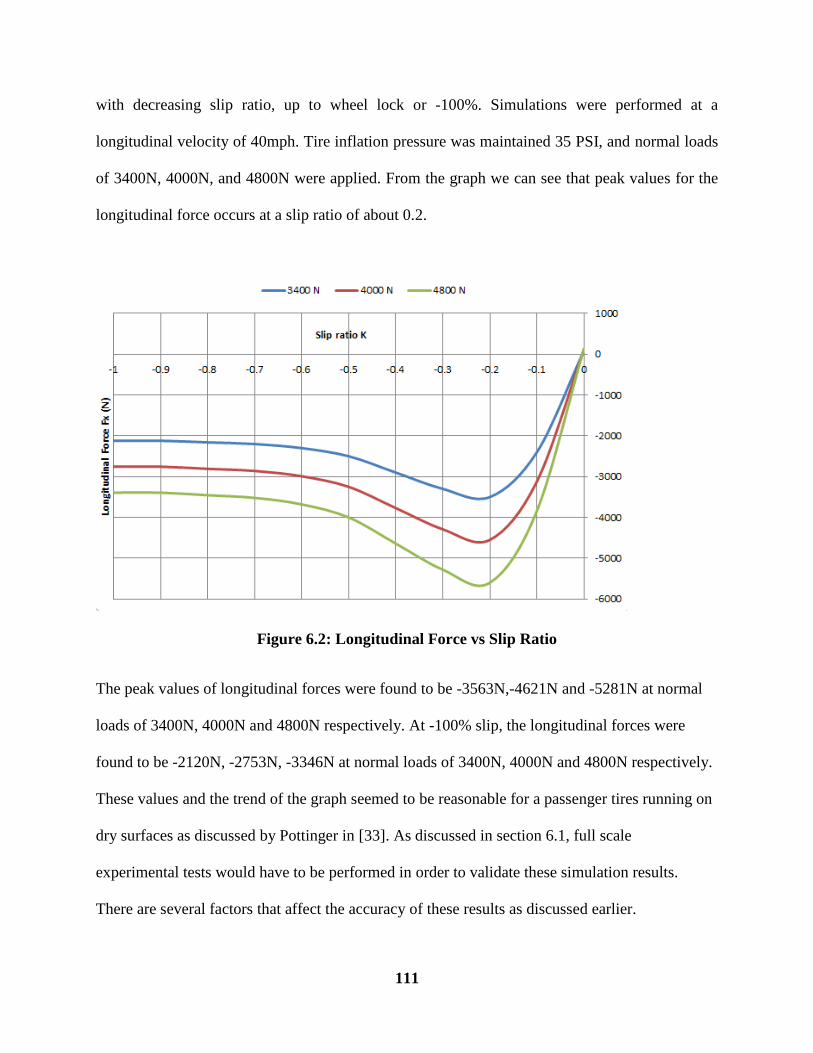
111
with decreasing slip ratio, up to wheel lock or -100%. Simulations were performed at a
longitudinal velocity of 40mph. Tire inflation pressure was maintained 35 PSI, and normal loads
of 3400N, 4000N, and 4800N were applied. From the graph we can see that peak values for the
longitudinal force occurs at a slip ratio of about 0.2.
Figure 6.2: Longitudinal Force vs Slip Ratio
The peak values of longitudinal forces were found to be -3563N,-4621N and -5281N at normal
loads of 3400N, 4000N and 4800N respectively. At -100% slip, the longitudinal forces were
found to be -2120N, -2753N, -3346N at normal loads of 3400N, 4000N and 4800N respectively.
These values and the trend of the graph seemed to be reasonable for a passenger tires running on
dry surfaces as discussed by Pottinger in [33]. As discussed in section 6.1, full scale
experimental tests would have to be performed in order to validate these simulation results.
There are several factors that affect the accuracy of these results as discussed earlier.

112
6.3.2. Pure Cornering Characteristics
As discussed earlier, pure cornering can be defined as the tire state that exists when the tire is at a
slip angle (negotiating a turn) in the free rolling condition, i.e. when no braking or tractive forces
are present at the contact patch. In order to simulate this condition in ABAQUS first the free
rolling solution is obtained and then another steady state step is included where the two slip
velocity components are defined. The angular velocity of the wheel is maintained at the free
rolling velocity.
Lateral force Generation:
Figure 6.3: Lateral force vs Slip Angle
The objective of this simulation is to determine the forces and moments generated at varying slip
angles and normal loads. Figure 6.3 shows the how the lateral force varies with slip angle at
different normal loads for the test tire. Simulations were performed at normal loads of 3400N,
4000N and 4800N. It also can be observed that at 𝛼 < 2.50 the lateral force increases linearly.

113
This is a typical characteristic of a tire [33]. The slope of this region is called cornering
stiffness 𝐶𝛼 and it is evident that the cornering stiffness depends on the applied load. This is a
very important parameter in determining the linear range behavior of the tire, as this is the region
where most driving is done. The cornering stiffness at normal loads of 3400N, 4000N and 4800
were found to be 2182 N/deg., 2567 N/deg and 3080.6 N/deg respectively.
Figure 6.4: Cornering Stiffness vs Normal Load
As seen from figure 6.4, the cornering stiffness depends on the applied normal load. It can also
be seen that it linearly increases up to a certain fraction, and then gradually falls off in magnitude
as load continues to increase [33]. Here the cornering stiffness was found to peak around 8000N,
(130% of the rated tire load) for the test tire. This parameter again depends on the on the tire
design. For good handling, it is desirable that the peak occurs at or above tire rated load [33], and
this is evident for the test tire.
From figure 6.3, we can also see that the increase in lateral force with slip angle is a complex
non-linear function. The lateral force peaks and then declines in a similar way to that for a tire
subject to longitudinal braking, however the transition from the peak is rather gradual. As slip
114
angle increases, more of the available contact area starts sliding, thus, a maximum or peak
amount of lateral force will be generated at some slip angle. Beyond the slip angle associated
with the peak, increasing the slip angle would cause a slight decrease in the lateral force
generated [33]. As discussed in section 6.1, full scale experimental tests would have to be
performed in order to check the veracity of these simulation results. There are several factors that
affect the accuracy of these results as discussed earlier.
Aligning moment:
As noted earlier the lateral force is a function of the slip angle. This gives rise to a moment
around the z-axis, which is known as the self-aligning moment. This is described by the
following equation as noted by Pacejka [32]:
𝑴𝒛 = −𝒕𝑭𝒚 + 𝑴𝒛𝒓 (6.5)
Where:
𝑡 = Pneumatic trail;
𝑀𝑧𝑟 = Small residual torque
Figure 6.5 shows how the self-aligning moment varies with slip angle and normal load at a speed
of 40mph. The inflation pressure again was maintained at 35PSI. It can be seen that the aligning
moments first increases and then decreases, with increasing slip angle. This is a typical
characteristic again as noted by Pottinger [33]. The location of the lateral force resultant moves
towards the origin of the reference coordinate system for increasing slip angle [32] and the
pneumatic trail thus decreases with increasing slip angle. The pneumatic trail can decrease even
move ahead of the origin at very large slip angles, such that the sign of the self-aligning moment
changes. As discussed in section 6.1, it is very important that full scale experimental tests are be
performed in order to validate these simulation results.

115
Figure 6.5: Aligning moment vs Slip Angle at 40mph
The effect of Conicity and Ply-Steer:
A close-up of the linear regions of the lateral force and aligning force vs slip angle is shown in
figure 6.6 and figure 6.7. It can be seen that both the lateral forces and self-aligning moments at
zero degree slip angle are nonzero.
Figure 6.6: Close-up view of the lateral force vs small slip angle
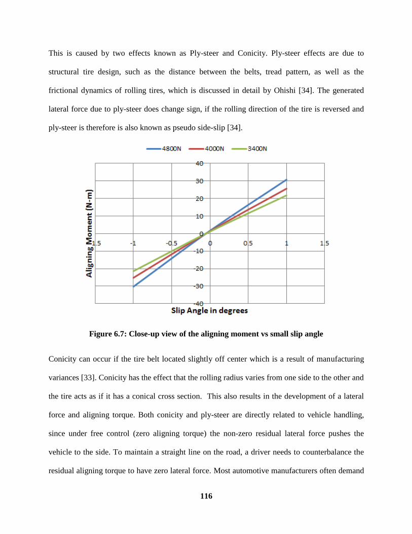
116
This is caused by two effects known as Ply-steer and Conicity. Ply-steer effects are due to
structural tire design, such as the distance between the belts, tread pattern, as well as the
frictional dynamics of rolling tires, which is discussed in detail by Ohishi [34]. The generated
lateral force due to ply-steer does change sign, if the rolling direction of the tire is reversed and
ply-steer is therefore is also known as pseudo side-slip [34].
Figure 6.7: Close-up view of the aligning moment vs small slip angle
Conicity can occur if the tire belt located slightly off center which is a result of manufacturing
variances [33]. Conicity has the effect that the rolling radius varies from one side to the other and
the tire acts as if it has a conical cross section. This also results in the development of a lateral
force and aligning torque. Both conicity and ply-steer are directly related to vehicle handling,
since under free control (zero aligning torque) the non-zero residual lateral force pushes the
vehicle to the side. To maintain a straight line on the road, a driver needs to counterbalance the
residual aligning torque to have zero lateral force. Most automotive manufacturers often demand

117
a specific range of ply-steer residual aligning torques, which is taken into account in the overall
vehicle design to reduce tire-induced pull effects. This can lead to different tire designs for a
nominally identical tire and as a result pull problems can occur if the original equipment tires are
replaced [10].

118
7.
CONCLUSION
7.1. Conclusions:
In conclusion:
i. An experimental procedure which has the capabilities to measure the footprint shape and
the normal pressure distribution at the contact patch with excellent resolution in both the
static condition and at slow rolling speeds was developed. However, this method records
only the peak stresses around the contact patch, and gives no indication about the change
in stresses in the dynamic conditions. Also, the maximum pressure limit this particular
film can record is 0.75MPa. Beyond this limit, a different film would need to be used.
This is another limitation about using this technique.
ii. The developed reverse engineering process used to create the finite element tire model
seems to provide reasonable results related to the footprint shape and normal pressure
distribution. However, this method does not have the ability to accurately predict the
distribution of the contact stresses at the contact patch. It gives a very good indication of
the peak stress levels and the footprint shape. A lot of information can be learnt by just
looking at the shape of the contact patch, and this model is able to accurately predict the
contact patch shape very well. Unfortunately, without the layout drawing and the detailed
material properties it would be very difficult to match the experimental and simulation
results.
iii. For the FE analysis of the tire, the commercial finite element package ABAQUS is used.
The steady-state transport analysis of ABAQUS is an efficient method to obtain the

119
footprint characteristics and the global steady-state force and moment characteristics of a
tire under different driving conditions. However, this method has also some limitations.
The underlying road must be flat and fully coupled thermo-mechanical simulations are
not possible in the current implementation. The choice for the improved friction model is
based on an overview of friction models to describe the frictional response of rubber,
while taking the limitations of the numerical method into account. The implemented
friction model uses empirical coefficients taken from research papers. In order to get
accurate values, friction experiments would need to be performed.
7.2. Scope for future work:
The finite element tire model capabilities are limited by the tire geometry and material properties
used. In future, if the layout drawing and the material properties for the test tire used can be
obtained from Michelin, this would be a great tool to use to check to see if the 2D layout and
material properties derived from the reverse engineering process concur. This would be very
useful information in order to completely implement this method in future. With this as a
reference, more complex tire models can be developed in order to predict tire wear. The
implemented friction model can be worked on as well and experiments would need to be
conducted in order to verify the constants used in this model. The predictive capability of the tire
model in combination with the fully identified friction model has been assessed. In future, if the
magic formula coefficients for this tire can be obtained, it would of great use to make a
comparison has been made between predicted handling characteristics of the finite element
model and using Pacejka’s magic formula to obtain the handling characteristics. For both, pure
cornering and braking, the forces and moments seem to be reasonably comparable with
literature. However this needs to be validated through experimental testing. This current FE

120
model developed is only for dry road simulation purposes. The friction model used, does not take
into account temperature variations. The temperature during frictional sliding of rubber is not
constant. Therefore, it is recommended to incorporate temperature effects in the FE model based
on the shear power intensity.

121
REFERENCES
[1] N. D. Smith, "Understanding Parameters Influencing Tire Modeling," Colorado State
University, 2003.
[2] A. N. Gent and J. D. Walter, The Pneumatic Tire, Akron: National Highway Traffic Safety
Administration, 2016.
[3] Continental, "History of the Tire," [Online]. Available: http://www.continental-
truck.com/truck/company/business-unit/tirehistory. [Accessed 02 09 2016].
[4] "Revzilla," [Online]. Available: http://www.revzilla.com/common-tread/why-things-are-
bias-ply-and-radial-tires. [Accessed 28 09 2016].
[5] M. Ghorieshy, "A state of the art review of the finite element modelling of rolling tyres,"
Iranian Polymer Journal, vol. 17, no. 8, p. 571–597, 2008.
[6] D. Beach and J. Schroeder, "An Overview of Tire Technology," Rubber World, vol. 222,
no. 6, pp. 44-53, 2000.
[7] B. E. Lindenmuth, "An overview of tire technology," in The Pneumatic Tire, Akron,
NHSTA, 2005, pp. 1-27.
[8] E. Bakker, L. Nyborg and H. Pacejka, Tyre modelling for use in vehicle dynamics studies,
SAE 870421, 1987.
[9] M. Pottinger, "Contact Patch (Footprint) Phenomena," in The Pneumatic Tire, Akron,
NHSTA, 2005, pp. 231-286.
[10] M. G. Pottinger, "The Three-Dimensional Contact Patch Stress Field of Solid and
Pneumatic Tires," Tire Science and Technology, vol. 20, no. 1, pp. 3-32, 1992.
122
[11] TekScan, "TireScan CrossDrive System," [Online]. Available:
https://www.tekscan.com/products-solutions/systems/tirescan-crossdrive-system. [Accessed
03 09 2016].
[12] C. R. Gentle, "Optical Mapping of Pressures in the Tyre Contact Patch," Optics and Lasers
in Engineering, vol. 4, pp. 167-176, 1983.
[13] 3. Simulia, "Abaqus 6.14 Online Documentation," Dassault Systèmes, 2014.
[14] U. Nackenhorst, " The ALE-formulation of bodies in rolling contact theoretical foundations
and finite element approach," Computer Methods in Applied Mechanics and Engineering,
vol. 193, pp. 4299-4322, 2004.
[15] J. Padovan, A. Kazempour, F. Tabaddor and B. Brockman, "Alternative formulations of
rolling contact problems," Finite Elements in Analysis and Design, vol. II, pp. 275-284,
1992.
[16] K. Rao, R. Kumar and P. Bohara, "Transient Finite Element Analysis of Tire Dynamic
Behavior," Tire Science and Technology, pp. 104-127, 2003.
[17] K. Kabe and M. Koishi, "Tire Cornering Simulation Using Finite Element Analysis,"
Journal of Applied Polymer Science, vol. 78, pp. 1566-1572, 2000.
[18] N. Balaramakrishna and R. K. Kumar, "A study on the estimation of SWIFT model
parameters by finite element analysis," Journal of Automobile Engineering , vol. 223, pp.
1283-1300, 2009.
[19] A. N. Gent, "Elasticity in Engineering with Rubber," New York: Hanser Publishers , 1992.
[20] G. Chagnon, G. Markmann and E. Verron, "A Comparison of the Hart-Simith Model with
Arruda-Boyce and Gent Formulations for Rubber Elasticity," Rubber Chemistry and

123
Technology , vol. 77, pp. 724-735 , 2004.
[21] A. Gent, "Relation between indentation Hardness and the Youngs modulus," IRI Trans, vol.
34, pp. 46-57, 1958.
[22] Y. Guan, G. Zhao and G. Cheng, "Influence of Belt Cord Angle on a Radial Tire under
Different Rolling States," Journal of Reinforced Plastics and Composites, vol. 25, no. 10,
pp. 1059-1077, 2006.
[23] R. V. D. Steen, "Tire-Road Friction Modeling," Eindhoven University of Technology ,
2007.
[24] A. Savkoor, "Dry adhesive friction of elastomers," Technische Universiteit Delft., 1987.
[25] H. Lupker, F. Cheli, F. Braghin, E. Gelosa and A. Keckman, "Numerical Prediction of Car
Tire Wear," Tire Science and Technology, vol. 32, no. 3, pp. 164-186, 2004.
[26] K. R. Smith, R. H. Kennedy and S. B. Knisley, "Prediction of Tire Profile Wear by Steady-
State FEM," Tire Science and Technology, vol. 36, no. 4, pp. 290-303, 2008.
[27] "Prescale," Fujifilm, [Online]. Available:
http://www.fujifilm.com/products/prescale/prescalefilm/#See_All. [Accessed 08 30 2016].
[28] "Fujifilm Prescale," Sensor Products Inc., [Online]. Available:
http://www.sensorprod.com/fuji-prescale.php. [Accessed 08 30 2016].
[29] P. Backx, "Tyre/Road contact measurement using pressure sensitive films," Technische
Universiteit Eindhoven , Eindhoven, 2007.
[30] P. Yap, Truck tire types and contact stresses, Kelowna, British Columbia: Goodyear, 1989.
[31] R. V. D. Steen, "Enhanced friction modeling for steady-state rolling tires," Eindhoven
University of Technology, Eindhoven, The Netherlands, 2010.

124
[32] H. Pacejka, Tyre and vehicle dynamics, Butterworth-Heinemann, 3rd Edition, 2006.
[33] M. G. Pottinger, "Forces and Moments," in The Pneumatic Tire, Akron, NHTSA, 2006, pp.
288-359.
[34] K. Ohishi, H. Suita and K. Ishihara, "The Finite Element Approach to Predict the Plysteer
and Residual Cornering Force of Tires," Tire Science and Technology, vol. 30, no. 2, pp.
122-133, 2002.
[35] Simulia, "An Integrated Approach for Transient Rolling of Tires," in Abaqus Technology
Briefing, 2007.
[36] P. Wriggers, "Computational contact mechanics," Springer, 2006.