DEVELOPING A SLAM-BASED BACKPACK MOBILE MAPPING SYSTEM FOR INDOOR MAPPING

Samer Karam

DEVELOPING A SLAM-BASED BACKPACK MOBILE MAPPING SYSTEM FOR INDOOR MAPPING

DISSERTATION

to obtain the degree of doctor at the University of Twente,

on the authority of the rector magnificus, prof.dr.ir. A. Veldkamp,

on account of the decision of the Doctorate Board, to be publicly defended

on Wednesday, October 27, 2021 at 14:45

by

Samer Karam

born on the 1st of January, 1989 in Idleb, Syrian Arab Republic

This thesis has been approved by Prof.dr.ir. M.G. Vosselman, supervisor Dr. V.V. Lehtola, co-supervisor ITC dissertation number 404 ITC, P.O. Box 217, 7500 AE Enschede, The Netherlands ISBN 978-90-365-5256-1 DOI 10.3990/1.9789036552561 Cover designed by Job Duim and Samer Karam Printed by CTRL-P, Hengelo © 2021 Samer Karam, The Netherlands. All rights reserved. No parts of this thesis may be reproduced, stored in a retrieval system or transmitted in any form or by any means without permission of the author. Alle rechten voorbehouden. Niets uit deze uitgave mag worden vermenigvuldigd, in enige vorm of op enige wijze, zonder voorafgaande schriftelijke toestemming van de auteur.

Graduation committee: Chairman/Secretary Prof.dr. F.D. van der Meer Supervisor(s) Prof.dr.ir. M.G. Vosselman University of Twente / ITC Co-supervisor(s) Dr. V.V. Lehtola University of Twente / ITC Members Prof.dr. M.J. Kraak University of Twente / ITC-GIP Dr. F.C. Nex University of Twente / ITC-EOS Prof.dr. J. Li University of Waterloo, Canada Prof.dr. A. Kukko Aalto University, Finland

i

Summary Indoor mobile mapping is important for a wide range of applications such as indoor navigation and positioning, mapping hazardous sites, facility management, virtual tourism and interior design. State-of-the-art indoor mobile mapping systems use a combination of light detection and ranging (LIDAR) scanners, cameras and/or inertial measurement units (IMUs) mounted on movable platforms and allow for capturing 3D data of buildings’ interiors. As global navigation satellite system (GNSS) positioning does not work inside buildings, the extensively investigated simultaneous localisation and mapping (SLAM) algorithms seem to offer a suitable solution for the problem. In this dissertation, a SLAM-based backpack mobile mapping system (ITC-Backpack) was developed for mapping buildings’ interiors. The configuration of the ITC-Backpack consists of three 2D LIDAR scanners and an IMU. The employed SLAM is planar feature-based SLAM algorithm that exploits the LIDAR scanners and the IMU to estimate the 3D pose and plane parameters. Representing the SLAM map by planes is advantageous for multiple reasons. First, the planar features are typically large and spatially distinct and therefore distinguishable from one another. Second, they are abundant in indoor man-made environments. Third, storing planar features takes less data space than storing the captured point clouds. Finally, the representation by planar shapes is a popular format for the state-of-the-art indoor 3D reconstruction methods. The developed SLAM in this dissertation performs loop closure detection and correction using these planar features. This enables the backpack system to recognize an already visited place and correct for the accumulated drift. The outputs of ITC-Backpack are reconstructed 3D planes, 3D point clouds as well as a trajectory of the system’s motion in a local coordinate system. A combination of the point cloud and the trajectory represents an advantageous supplementary information for some indoor modelling problems such as semantic interpretation and space partitioning. The ITC-Backpack system is validated on various indoor environments that differ in terms of geometry, architecture and clutter. Moreover, we evaluate the performance of the system by comparing the obtained point clouds against those obtained from a commercial indoor mobile mapping system, Viametris1 iMS3D, and ground truth obtained from a terrestrial laser scanner (TLS).

1 www.viametris.com

Summary

ii

iii

Samenvatting Indoor mobile mapping is belangrijk voor een breed scala aan toepassingen, zoals indoor navigatie en positionering, het in kaart brengen van gevaarlijke locaties, facility management, virtueel toerisme en interieurontwerp. Geavanceerde mobiele karteringssystemen voor binnenshuis maken gebruik van een combinatie van lichtdetectie- en afstandsscanners (LIDAR), camera's en/of traagheidsnavigatiesystemen (IMU's) die op verplaatsbare platforms zijn gemonteerd en maken het mogelijk om 3D-gegevens van het interieur van gebouwen vast te leggen. Omdat plaatsbepaling met het Global Navigation Satellite System (GNSS) niet werkt binnen gebouwen, lijken de uitgebreid onderzochte algoritmen voor simultaneous localisation and mapping (SLAM) een geschikte oplossing te bieden voor het probleem. In dit proefschrift is een op SLAM gebaseerd mobiel karteringssysteem voor een rugzak (ITC-rugzak) ontwikkeld voor het in kaart brengen van interieurs van gebouwen. De configuratie van de ITC-rugzak bestaat uit drie 2D LIDAR scanners en een IMU. De gebruikte SLAM is een op vlakken gebaseerd SLAM-algoritme dat gebruik maakt van de LIDAR-scanners en de IMU om de 3D positie en stand van de rugzak en de parameters van de vlakken in het interieur te schatten. De weergave van de SLAM-kaart door vlakken heeft verschillende voordelen. Ten eerste zijn de vlakken meestal groot en ruimtelijk gescheiden en dus goed van elkaar te onderscheiden. Ten tweede zijn ze in ruime mate aanwezig in binnenruimten. Ten derde neemt het opslaan van vlakken minder dataruimte in beslag dan het opslaan van de vastgelegde puntenwolken. Tenslotte is de representatie door vlakken een populair formaat voor de state-of-the-art indoor 3D reconstructiemethoden. De ontwikkelde SLAM in dit proefschrift voert lusdetectie en -correctie uit met behulp van deze vlakken. Dit stelt het rugzaksysteem in staat om een reeds bezochte plaats te herkennen en de opgelopen drift te corrigeren. De uitvoer van de ITC-rugzak zijn gereconstrueerde 3D vlakken, 3D puntenwolken en het afgelegde traject van het systeem in een lokaal coördinatenstelsel. De combinatie van de puntenwolk en het traject vormt waardevolle informatie voor sommige indoor modelleringsproblemen zoals semantische interpretatie en ruimte-indeling. Het ITC-Backpack systeem is gevalideerd op verschillende binnenomgevingen die verschillen in geometrie, architectuur en de hoeveelheid meubilair. Bovendien evalueren we de prestaties van het systeem door de verkregen puntenwolken te vergelijken met die verkregen met een commercieel mobiel

Samenvatting

iv

karteringssysteem voor gebruik binnenshuis, Viametris iMS3D, en referentiemetingen verkregen met een terrestrische laserscanner (TLS).

v

Acknowledgements Throughout my research journey, I have received wonderful support from my supervisors, friends and family. This work would not have been the same without each and every one of them. I thank them for every moment we shared and for the many lessons I have learnt from this journey. I would first like to thank my promoter and supervisor, George, who took my hand from the start of my PhD journey. I will be forever thankful for his support and guidance, which made me understand why the term “doctor father” is used. The combination of his enormous expertise, humble and direct supervision style and accurate, comprehensive feedback is and will be endlessly appreciated. I’m also very grateful to my former co-supervisor, Michael Peter, who provided significant support at the rough beginning and became a dear friend during this journey. This also applies to my other great former co-supervisor, Siavash Hosseinyalamdary. Last but not least, I thank my current co-supervisor, Ville Lehtola, for his thoughtful feedback that

my work and my knowledge. improved both Thanks to my dear friends and colleagues at the ITC faculty, starting with you, Sugandh: you have been one of my best friends in ITC, and I will never forget your cheerful way of pushing me to socialize during those times I was undoubtedly becoming a hermit. This also applies to you, Mila and Claudio: our chats and discussions always lifted my spirits. Whenever someone heard me chatting cheerfully in Arabic at the EOS department, it was with you, Shaheen and Yolla, my great friends. Thanks also to Sander, Francesco, Riyaz, Shayan, Zill, Fashuai, Ye, Yaping, Sofia, Tatjana, and Phillipp for the small but meaningful chats by the coffee machine and during ITC lunchtimes (before Covid-19 :( ). I would also like to express my appreciation to Teresa, our former EOS office manager, for her energetic attitude; Loes, the secretary of the graduate program, for her kindliness; Karen, human resources advisor, for her friendly assistance; Roelf for his smile every time I passed from the reception; Roland for his logistic support and Jenny for her lovely words and support at the end of my PhD. My appreciation also extends to Dr. Hussin, Dr. Alsadik and Dr. Salama. To everyone with whom I shared small talks, tea and lunch breaks, international events, and delicious food festivals, thank you for making my time at the ITC a memory to treasure. My parents are the foundation and reason for every step I make; words alone can’t describe how grateful I am for having you. The greatest gift you gave me was my brothers and sisters: Mohammed, Nisreen, Basel, Mariam, Ahmad, and Alaa. Thanks to my uncle and aunts for your care and support. Finally, a big thanks to my newphews and nieces, Abdulwahab, Muhammad, Taim, and Ward, who all provided a happy distraction from my research. Family is where

Acknowledgements

vi

we all start and end; without you all, all my efforts would have been meaningless. I would like to thank my partner and the smartest PhD candidate I know, my beloved fiancée, Dana, for all your continuous love and support from the bottom of my heart. You have shared every moment with me, whether it was a joyful or stressful one, and provided a listening ear in difficult situations. You were my refuge in every difficult situation I have been through. I’m looking forward to a lifetime together and being your number one supporter in your PhD journey and throughout life. My deepest gratitude to my second family in Germany: Helga-Jasmina, Adham, Hussam and Karim. Families comes in varying shapes and sizes, and some good friends count as a family when supporting us through difficult times. To Bara'a and Ghazwan, you both count as a family to me as you helped alleviate my hardships along the way. I would also like to thank my good friends, Muntagab, Omar, Ammar, Muhammad-Abdulhadi, Hassan, Imad, Ibrahim, Leo, Abid, Salem, Alaa, Fida and Ola for all the memorable moments we shared. Thanks to the German Academic Exchange Service (DAAD), which awarded me a scholarship that supported me during my Master’s studies in Germany. In particular, I thank Pia Schauerte from the bottom of my heart for all the support she provided both during and after the scholarship. The tremendous and well-organized DAAD events and conferences allowed me to meet many brilliant Syrian students and researchers spread all over Germany. Although I can not mention everyone here by name, I am very honored to know these great minds and proud of all the Syrians successfully contributing to academia. My thanks to the scientific staff for the Geomatics Engineering (GEOENGINE) Master’s program at the University of Stuttgart, including, but not limited to, Prof. Haala, Dr. Cramer and Prof. Fritsch. I also express my gratitude to the German Aerospace Center (DLR) for allowing me to join its distinguished research team in the field of photogrammetry and remote sensing. In particular, I would like to acknowledge Prof. Peter Reinartz, Dr. Tahmineh and Mrs. Sabine for their generous support. My appreciation also extends to the scientific staff of the Faculty of Civil Engineering at the University of Aleppo, including, but not limited to, Dr. Makdisi, Dr. Jibrini, Dr. Zakzok, Dr. Ramadan, Dr. Alamouri, Dr. Othman, Dr. Sarkis, Dr. Kbieh and Dr. Alkamouh whose assistance was pivotal to my academic career. My grateful and profound thanks to my doctor and friend, Dr. Sammuneh. I also wish to express my deepest gratitude to Dr. Roudineh, the kindest friend and boss I ever worked with. Thanks to all my friends and

Acknowledgements

colleagues in the Department of Topography Engineering for all the memorable moments during our Bachelor’s degree. I also want to take a moment to thank Paul: you have been one of my most cherished discoveries during my work at the University of Twente. I highly appreciate your concern about the Syrian issue and your knowledge of what is really going on there. Horse riding was not only a great opportunity to have a better work-life balance, but it also allowed me to meet lovely people who became dear friends: Evelien, Jasper, Linda, Vera, Hugo, Jannes, Eline and Gijs. I would also take the chance to express my gratefulness to my Turkish family, erkekkardeşler ve kızkardeşler, Pinar, Haydar, Niyazi, Hatice, Evren, Omar, Mustafa, Sercan and Khalil. Finally, I wish to dedicate this degree to a better future for my wounded home country, Syria, and its kind people after the present injustices and tyranny have departed. I believe that science and knowledge are the only way for a brighter tomorrow.

Acknowledgements

viii

ix

Table of Contents Summary .................................................................................. i Samenvatting ............................................................................ iii Acknowledgements ..................................................................... v List of figures .......................................................................... xiii List of tables ............................................................................ xv Chapter 1 - Introduction ............................................................. 1

1.1 Background and Motivation ................................................ 2 1.2 Research Objectives ......................................................... 4 1.3 Research Questions .......................................................... 5 1.4 Dissertation Outline .......................................................... 6

Chapter 2 - State-of-the-art indoor mobile mapping systems .......... 9 2.1 Review of the state-of-the-art indoor mobile mapping systems ................................................................................ 10 2.1.1 Trolley-based Systems ................................................... 10 2.1.2 Hand-held Systems ........................................................ 12 2.1.3 Wearable Systems ......................................................... 13 2.2 Discussion and Conclusion ............................................. 16

Chapter 3 - Design, Calibration, and Evaluation of a Backpack Indoor Mobile Mapping System * .......................................................... 19

Abstract ................................................................................ 20 3.1 Introduction ................................................................. 21 3.2 Related Work ............................................................... 23 3.2.1 Hand-Held Systems ....................................................... 23 3.2.2 Backpack Mapping Systems ............................................ 24 3.2.3 Evaluation Methods ........................................................ 26 3.3 Backpack System ITC-Backpack ..................................... 26 3.3.1 System Description ........................................................ 26 3.3.2 Coordinate Systems ....................................................... 27 3.3.3 6DOF SLAM ................................................................... 29 3.4 Calibration Process ....................................................... 30 3.4.1 Calibration Facility ..................................................... 30 3.4.2 Calibration ................................................................ 30 3.4.3 Self-Calibrations ........................................................ 31 3.5 Relative Sensor Registration .......................................... 31 3.5.1 Initial Registration ......................................................... 32 3.5.2 Fine Registration ........................................................... 32 3.5.3 Self-Registration ............................................................ 34 3.6 SLAM Performance Measurements and Results ................. 34 3.6.1 Dataset ........................................................................ 34 3.6.2 Evaluation Techniques .................................................... 35 3.6.2.1 Evaluation Using Architectural Constraints ..................... 36 3.6.2.2 Evaluation Using a Floor Plan ........................................ 38

x

3.7 Determining Optimal Configuration ................................. 43 3.7.1 Studied Configurations ................................................... 43 3.7.2 Experimental Comparison of Configurations ...................... 45 3.7.2.1 Accuracy .................................................................... 45 3.7.2.2 Completeness of Data Capturing ................................... 47 3.7.3 Discussion of Configuration Experiments ........................... 48 3.8 Conclusions and Future Work ......................................... 49

Chapter 4 - Integrating a Low-Cost MEMS IMU Into a LIDAR SLAM for Indoor Mobile Mapping * ........................................................... 51

4.1 Introduction ................................................................. 53 4.2 Related Work ............................................................... 54 4.3 LIDAR SLAM And IMU Integration ................................... 55 4.3.1 System Components ...................................................... 55 4.3.2 Coordinate Systems and Registration Process .................... 55 4.3.3 LIDAR SLAM .................................................................. 56 4.3.4 IMU-based Pose Prediction .......................................... 57 4.3.4.1 Attitude ................................................................. 58 4.3.4.2 Position ................................................................. 58 4.3.5 SLAM and IMU Integration .......................................... 59 4.4 Datasets ...................................................................... 59 4.5 Analysis of IMU Performance .......................................... 60 4.5.1 IMU Data Analysis.......................................................... 60 4.5.2 IMU Prediction Analysis .................................................. 62 4.6 Integration Results And Discussion ................................. 63 4.7 Conclusions and Future Work ......................................... 67

Chapter 5 - Strategies to Integrate IMU and LIDAR SLAM for Indoor Mapping * ................................................................................ 69

5.1 Introduction ................................................................. 71 5.2 Related Work ............................................................... 73 5.3 IMU-SLAM Integration Strategies .................................... 74 5.3.1 IMU-SLAM Switching ...................................................... 75 5.3.2 IMU-based Pose Estimation ............................................. 76 5.3.3 IMU-SLAM Joint Estimation ............................................. 76 5.3.3.1 Acceleration Observation Equations ............................... 77 5.3.3.2 Angular Velocity Observation Equations ......................... 78 5.3.3.3 Joint Estimation .......................................................... 80 5.4 Experimental Results and Discussion ............................... 80 5.5 Conclusions And Future Work ......................................... 87

Chapter 6 - Simple loop closing for continuous LIDAR&IMU Planar Graph SLAM for 3D indoor environments * ................................... 89

6.1 Introduction ..................................................................... 91 6.2 Related Works .................................................................. 93 6.3 Methodology .................................................................... 94 6.3.1 Initialization .................................................................. 94 6.3.2 Planar Segment Extraction and Local SLAM Map Updating ... 95

6.3.3 State definition and Plane and Trajectory Parametrization ... 97 6.3.4 LIDAR observation equation ............................................ 98 6.3.5 IMU observation equation ............................................. 100 6.3.6 Local_SLAM ................................................................ 103 6.3.7 Global-SLAM and Autocalibration ................................... 104 6.3.8 Loop Closure Detection and Correction ........................... 105 6.4 Experiments .................................................................. 106 6.4.1 Mobile Mapping System ................................................ 106 6.4.2 Study Areas and Datasets ............................................. 106 6.4.3 Analysis of SLAM Performance ....................................... 108 6.4.4 Cloud to Cloud Comparison ........................................... 109 6.4.4.1 Comparison against a commercial mobile mapping system ......................................................................................... 113 6.4.4.2 TLS Comparison........................................................ 114 6.4.5 Discussion and Limitations ............................................ 114 6.5 Conclusions ................................................................... 116

Chapter 7 - Synthesis .............................................................. 119 7.1 Scope of application ....................................................... 120 7.2 Conclusions per objective ............................................... 121 7.3 Reflections and outlook .................................................. 124

Bibliography ........................................................................... 129 Author’s Biography ................................................................. 137

xii

List of figures

Figure 1.1. Dissertation outline .................................................... 8 Figure 2.1. state-of-the-art trolley-based IMMSs ........................... 11 Figure 2.2. state-of-the-art hand-held IMMSs ............................... 12 Figure 2.3. Wearable IMMSs ....................................................... 15 Figure 3.1. The laptop used and the backpack system. .................. 28 Figure 3.3. The residuals between the points and estimated planes . 37 Figure 3.4. The results of the architectural constraints method ....... 39 Figure 3.5. The digitized floor plan and point cloud-based edges ..... 39 Figure 3.6. The final point cloud edges ........................................ 40 Figure 3.7. Errors in angle as relation of distance .......................... 41 Figure 3.8. All edge pairs that have an angle error of 3˚ or more. ... 42 Figure 3.9. Errors in distance in relation to the distance................. 43 Figure 3.10. Part of the 2D CAD drawing of the 3rd floor ............... 46 Figure 3.11. Simulation data. ..................................................... 48 Figure 4.1. The backpack system ................................................ 56 Figure 4.2. An example plot for testing the IMU integration. ........... 62 Figure 4.3. Part of the rotation angles (ω, κ) trajectories. .............. 64 Figure 4.4. A top view of the generated point cloud by SLAM.......... 65 Figure 4.5. Histograms of the points’ residuals ............................. 66 Figure 5.1. The used laptop and the current backpack system ........ 72 Figure 5.2. An exemplary representation of the prediction and adjustment processes within SLAM. ............................................ 75 Figure 5.3. An example of a problematic area for the LiDAR SLAM.. 82 Figure 5.4. The generated point cloud of the test areas. ................ 84 Figure 5.5. Histograms of the points’ residuals ............................. 85 Figure 6.1. The overall concept of the loop-closing LIDAR-IMU SLAM system .................................................................................... 95 Figure 6.2. Planar segment extraction. ........................................ 96 Figure 6.3. The loop closure schematic ...................................... 106 Figure 6.4. Mobile mapping system (ITC Backpack). ................... 108 Figure 6.5. Slanted view of the generated point clouds of the ITC building datasets. ................................................................... 111 Figure 6.6. Top view and slanted view of the generated point clouds of the Fire Brigade building datasets ......................................... 112 Figure 6.7. The first-floor loop in the ITC building ....................... 113 Figure 6.8. ITC-Backpack and Viametris iMS3D comparison. ........ 113 Figure 6.9. ITC-Backpack and TLS comparison. .......................... 114 Figure 6.10. Point cloud of part of the third and second floor in the ITC building ........................................................................... 116

xiv

List of tables

Table 3.1. Values of mean, standard deviation, and the number of edges pairs .............................................................................. 42 Table 3.2. Tested configurations. ................................................ 45 Table 4.1. RMSE values of all the predicted pose parameters ......... 63 Table 4.2. The number of assigned points and the corresponding RMSEs of the residuals. ............................................................. 65 Table 4.3. Percentages of angles’ errors for parallelism and perpendicularity in two cases, SLAM with and without IMU. ............ 66 Table 4.4 RMSE of angles’ errors for parallelism and perpendicularity in two cases, SLAM with and without IMU .................................... 67 Table 5.1. Key specifications of the Xsens MEMS IMU .................... 77 Table 5.2. Comparison between the proposed methods ................ 81 Table 5.3. Comparison between the performance of the proposed method on all datasets .............................................................. 85 Table 5.4. Comparison between the performance of the proposed method on all datasets regarding the architectural constraints ....... 86 Table 6.1. General information about captured datasets .............. 110

xvi

1

Chapter 1 - Introduction

Introduction

2

1.1 Background and Motivation

During the last years, the scope of indoor mapping has widened to many important applications such as mapping hazardous sites, indoor navigation, and virtual tourism. Since digital maps of public buildings (airports, hospitals, train stations, etc.) are a prerequisite for several location-based services and applications such as navigation and facility management, there will be a trend towards the development of indoor applications using geospatial data (Norris, 2013). This importance for the mapping of building interiors has encouraged scientists to focus on improving the mapping techniques for such environments. Traditional methods to map building interiors fundamentally depended on total stations (TS) or terrestrial laser scanning (TLS) (Thomson et al., 2013). However, those techniques are no more applicable when we deal with complex indoor environments since they would require setting up the TS/TLS at many different positions, which is time-consuming and makes data collection laborious (Maboudi et al., 2018; Salgues et al., 2020). In order to map such environments, indoor mobile mapping systems (IMMSs) are needed. While outdoor mobile mapping systems are widely available, indoor mobile mapping has remained a challenge as global navigation satellite systems (GNSSs) do not work indoors. Simultaneous localisation and mapping (SLAM) algorithms offer reasonable positioning estimates in environments where satellite positioning is not available (Salgues et al., 2020). Therefore, group of SLAM algorithms are extensively investigated for indoor map generation. The IMMS is generally a kinematic platform that is composed of sensors suitable to localize the system and map the environment simultaneously. Commonly used sensors can be classified into navigation sensors such as Inertial Measurement Units (IMUs) and sensors that collect information of the system’s environment such as light detection and ranging (LIDAR) scanners and cameras. The usual outputs of IMMSs are images and/or 3D point clouds as well as a trajectory of the system’s motion in a local coordinate system. In order to retrieve the location of the platform, IMMSs primarily make use of some SLAM algorithm for the purpose. A wide range of indoor mobile mapping systems have been developed in recent years. These systems can be categorized into: hand-held systems such as ZEB1 (Bosse et al., 2012) and ZEB REVO1, trolley-based systems such as

1 www.geoslam.com

Chapter 1

3

Trimble1 TIMMS, NavVis2 M6, Viametris3 i-MMS and iMS3D and wearable – mostly backpack-based – systems (Cinaz & Kenn, 2008; Filgueira et al., 2016; Kim, 2013; Liu et al., 2010; Naikal et al., 2009; Wen et al., 2016; Blaser et al., 2019). Although a lot of efforts have been exerted in designing indoor mobile mapping systems and developing localization and mapping algorithms, designing an accurate and versatile SLAM-based IMMS has still remained a challenge. The trolley-based systems are often more accurate than the other two categories, but they are more expensive (Otero et al., 2020). Furthermore, the trolley-based systems do not have the ability to access the entirety of interior areas such as staircases. Therefore, they need an alignment process of the point clouds from different floors, and this requires more effort. The advantage of hand-held and wearable mapping systems over other IMMSs is that they can move in a more flexible way and are faster for data acquisition. Most mapping systems that depend on SLAM for localization instead of GNSS and IMU cannot be operated in all types of buildings. For instance, Viametris i-MMS is only able to map in an environment with a small variance in height because of its reliance on 2D SLAM in positioning. Furthermore, assumptions that SLAM algorithms are built on can constrain them. For instance, some algorithms require the floor to be planar (Chen et al., 2010). Other SLAM algorithms can only work in buildings with a Manhattan world architecture (Flint et al., 2011). On the hardware side, SLAMs that employ one type of sensor (camera, LIDAR, or IMU) for indoor navigation have limitations. For instance, camera-based SLAM (Visual SLAM) searches for similar features in consecutive images. Consequently, Visual SLAM is prone to failure if the environment lacks visual features. Moreover, the camera-based IMMSs need to move slowly in order to avoid blurred images. Also, the light conditions in indoor environments may not be good enough to capture high-quality images. Therefore, it is better to use an active sensing-based mapping system for indoor environments. The laser scanner-based SLAM (LIDAR SLAM) depends basically on the association between the successive scans, where scan here refers to the set of points that is captured by the LIDAR scanner each sweep. However, LIDAR SLAM fails if the geometry of LIDAR observations is not strong enough to reliably estimate the 3D pose of the mapping system. IMU sensor suffers from accumulated errors over time, which makes it undesirable as a stand-alone sensor for navigation.

1 www.trimble.com 2 www.navvis.com 3 www.viametris.com

Introduction

4

One of the fundamental steps in any SLAM algorithm is to determine the correspondences between the recently observed data by sensors and the up-to-date built map in SLAM, the so-called data association process. Moreover, loop closure is one of the key difficulties hampering SLAM because recognizing previously visited places requires searching through all the collected data, which becomes computationally expensive over time.

1.2 Research Objectives In the light of the above information, the main objective of this research is to design a wearable indoor mobile mapping system (IMMS) – ITC-Backpack – that utilizes a combination of laser range-finders (LRFs) – 2D scanners – and an IMU to fully recover a 3D point cloud of building interiors based on a feature-based SLAM algorithm. Specifically, we use planar features, which are advantageous due to their large size and dominant existence in indoor man-made environments. Moreover, the outcome of this research will be a SLAM system that inherently performs loop closure detection and correction using planar features. Furthermore, we try to keep the system design as inexpensive as possible by making use of simple LRFs and a relatively low-cost IMU. Sub-objectives are:

1) To find the optimal configuration of the LRFs of the designed system to avoid occlusion and acquire sufficient geometrical information of buildings.

2) To integrate the IMU with LIDAR into SLAM so that we exploit the strength of the scanning geometry for accurate positioning in 3D and the strength of the IMU in measuring short-term pose changes.

3) To develop a hypothesis generation of arbitrarily oriented planar structures. This enables the backpack system to map some complex spaces such as staircases and fancy architecture (e.g., slanted walls, sloping floor, ..etc).

4) To develop a reliable data association that defines the correspondences

between the recently observed data by sensors and the up-to-date built map in SLAM.

5) To integrate a loop closure detection and correction technique with the

LIDAR-IMU SLAM system so that the system becomes able to recognize an already visited place and correct the accumulated drift by then.

6) To develop an evaluation pipeline for indoor laser scanning point

clouds.

Chapter 1

5

1.3 Research Questions The research questions, which the methodology should be able to answer, are derived and classified based on the objectives of this research. System design

1) What is the optimal configuration for the scanners in terms of the success of SLAM, completeness of the resulting point cloud and the reconstruction accuracy?

Integrating IMU with the LIDAR SLAM

1) What is the best method for pose prediction?

2) How good is the performance of IMU and how long can the system rely on it for positioning?

3) How to combine the IMU and LIDAR in order to participate in 3D pose estimation?

4) What is the optimal strategy for IMU-LIDAR SLAM integration? Hypothesis of planar structures

1) How to make a hypothesis for an arbitrarily oriented plane?

2) How can the IMU be utilized to generate a reliable hypothesis of planar

structures? Data association

1) What is the most efficient and reliable way for data association?

2) How can the points, which do not belong to a segment, e.g., plane, be

exploited? Loop closure

1) How can the mapping system recognize a revisited place after visiting large unknown areas?

2) How big is the accumulated drift at the end of a loop?

3) To what extent can the proposed SLAM handle the loop closure?

4) How to correct the accumulated drift and relocalize the mapping system in the SLAM map?

Introduction

6

Analysis and evaluation of the point cloud

1) How to check the internal consistency of the reconstructed map?

2) How to evaluate the quality of the acquired point cloud?

3) How can this evaluation be done in the absence of any ground truth model?

4) How to get an overall impression of the reconstruction accuracy?

5) What is the performance of the developed IMMS compared to a commercial IMMS and a TLS?

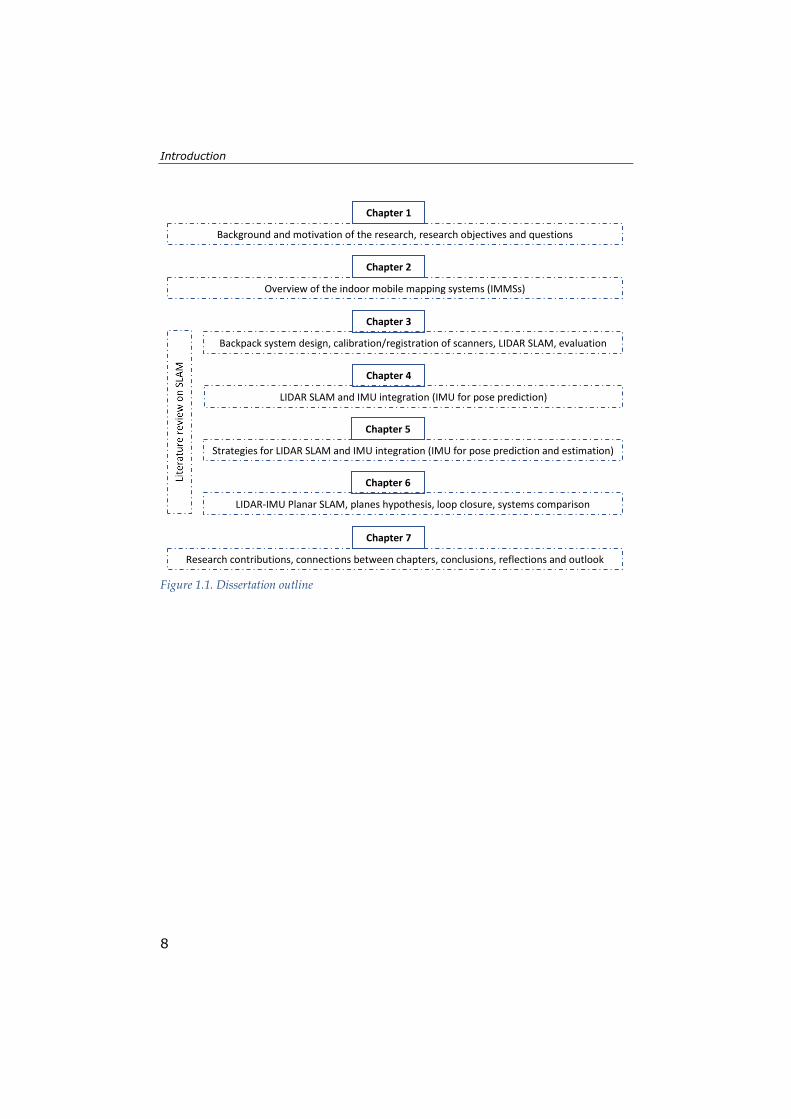
1.4 Dissertation Outline This dissertation consists of seven chapters (Figure 1.1), including an introduction, a literature review, four core chapters and a synthesis. The dissertation from Chapter 3 to Chapter 6 shows the progress in the development of the ITC-Backpack mobile mapping system. These chapters are based on publications (see the first page of each chapter) and cover the literature review on SLAM, sometimes with a bit of overlap. A complementary overview of the indoor mobile mapping systems (IMMSs) is provided in Chapter 2. Chapter 1: introduces the background and the motivation of the research, in addition to the research objectives and questions. This chapter also describes the dissertation outline. Chapter 2: presents an overview of the state-of-the-art IMMSs. The state-of-the-art SLAM algorithms are discussed in the subsequent chapters. Chapter 3: presents the design of the ITC-Backpack and the employed planar feature-based LIDAR Graph SLAM algorithm that utilizes a combination of three laser range-finders (LRFs) to fully recover the 3D building map. The calibration process of the mounted LRFs is explained in this chapter. Moreover, this chapter introduces an evaluation pipeline for indoor laser scanning point clouds. Chapter 4: investigates the benefits that the integration of a low-cost microelectromechanical system (MEMS) IMU can bring to the planar feature-based LIDAR Graph SLAM. Specifically, we utilize IMU data to predict the pose of our backpack indoor mobile mapping system to improve the SLAM algorithm. The performance of the proposed IMU integration method is tested on a dataset acquired in a distinct office environment at the Institute of Geodesy and Photogrammetry building at the University of Braunschweig, Germany.

Chapter 1

7

Chapter 5: proposes further strategies that utilize the benefits of the IMU in the pose estimation and support the LIDAR SLAM in overcoming some pathological pose configurations. The proposed strategies are again tested using different datasets collected at the Institute of Geodesy and Photogrammetry building at the University of Braunschweig, Germany. Chapter 6: presents a loop-closing LIDAR-IMU Graph SLAM for indoor environments. The design of the proposed SLAM is based on locally-generated planar features that can be matched against one another to perform local but also global optimization. Hence, this design allows for a simple global loop closing technique – a main contribution of this work. This chapter presents also how the IMU is exploited to predict the pose of a few successive LIDAR scans. This allows for the generation of a reliable hypothesis of planar structures, which in turn allows SLAM to handle indoor environments with arbitrarily oriented planes such as staircases. The proposed method is validated on the ITC-Backpack system and the generated point clouds are compared against ones obtained from a commercial mobile mapping system (Viametris iMS3D) and a terrestrial laser scanner (RIEGL VZ-400). The data is collected from two buildings that differ in terms of geometry, architecture and cluttering in general. Chapter 7: discusses the research contributions, connections between chapters, to what extent the objectives were achieved, the main conclusions of the carried out research and recommendations for future research.

Introduction

8

Figure 1.1. Dissertation outline

Background and motivation of the research, research objectives and questions

Chapter 1

Overview of the indoor mobile mapping systems (IMMSs)

Chapter 2

Backpack system design, calibration/registration of scanners, LIDAR SLAM, evaluation

Chapter 3

LIDAR SLAM and IMU integration (IMU for pose prediction)

Chapter 4

Strategies for LIDAR SLAM and IMU integration (IMU for pose prediction and estimation)

Chapter 5

LIDAR-IMU Planar SLAM, planes hypothesis, loop closure, systems comparison

Chapter 6

Research contributions, connections between chapters, conclusions, reflections and outlook

Chapter 7

9

Chapter 2 - State-of-the-art indoor mobile mapping systems

State-of-the-art indoor mobile mapping systems

10

2.1 Review of the state-of-the-art indoor mobile mapping systems Indoor data acquisition systems have a dramatic progress in the past few years. Besides the existing static devices such as terrestrial laser scanners (TLS), a wide range of indoor mobile mapping systems (IMMSs) have been developed. Some of them are research systems and others are commercial with limited information of the solutions and performance published. In this chapter, we will provide a brief description of a selection of the state-of-the-art IMMSs (commercial and research prototypes) as related works to the current research. Three types of these IMMSs have prevailed so far: hand-held, trolley-based and wearable. 2.1.1 Trolley-based Systems Trolley-based systems provide a stable platform and avoid placing the burden of carrying the weight of the sensors onto the operator (Figure 2.1). This gives manufacturers more freedom to mount sensors disregarding their weight. For instance, the Slammer platform carries two terrestrial laser scanners (TLSs) and utilizes freely available simultaneous localization and mapping (SLAM) algorithm for indoor localization (Kaijaluoto et al., 2015). The Leica Proscan1 trolley (Figure 2.1a) carries one TLS as a mapping sensor and weighs 40 kg (Otero et al., 2020). Although Proscan looks similar to Trimble TIMMS2 (49.5 kg), it can not work with the same models of TLS. Proscan works with Leica ScanStation TLSs, while TIMMS works with different models of FARO TLS. However, both systems utilize an inertial measurement unit (IMU) sensor for positioning (Otero et al., 2020).

While Slammer, Proscan and TIMMS use 3D light detection and ranging (LIDAR) scanner (i.e., TLS), Viametris3 developed two versions of mapping trolley, i-MMS and iMS3D, in which 2D LIDAR scanners are used. The recent version iMS3D (12 kg) integrates three Hokuyo4 LIDAR scanners (single-layer) and a Ladybug panoramic camera (spherical pictures). Figure 2.1c clarifies the configuration of the three scanners with respect to each other. The Hokuyo scanner with an orange head (UTM-30LX) is mounted horizontally while the other two with blue heads (UTM-30LX-EW) are vertical and to the right and left of the horizontal one. Viametris utilizes the combination of LIDAR-based SLAM algorithm and an IMU for positioning and generating the point cloud of the surrounding environment (Viametris, 2021). In this research, we intend to compare point clouds generated by our developed backpack IMMS against ones obtained from iMS3D (see Chapter 6).

1 www.leica-geosystems.com 2 www.trimble.com 3 www.viametris.com 4 www.hokuyo.com

Chapter 2

11

(a) Leica Proscan1

(b) Trimble TIMMS2

(c) Viametris iMS3D3

(d) NavVis M34

(e) NavVis M64

Figure 2.1. state-of-the-art trolley-based IMMSs

1 www.leica-geosystems.com 2 www.trimble.com 3 www.viametris.com 4 www.navvis.com

State-of-the-art indoor mobile mapping systems

12

NavVis1 has also released two versions of a mapping trolley, M3 and M6, similar to Viametris trolley. The M3 Trolley is constructed from three Hokuyo (UTM-30LX) scanners, an IMU, six cameras (Figure 2.1d). Two of the scanners are mounted vertically for capturing the data on both sides of the system, while the third scanner is horizontal on the head unit and used for 2D localization and mapping. The six cameras also are mounted on the head unit to get a 360ᵒ coverage of the surrounding area during data collection. Compared to the M3, the recent version M6 (40 kg) has four scanners with different configuration as shown in Figure 2.1e. The Hokuyo scanners are tilted and distributed differently on the platform compared to the M3. The horizontal single-layer Hokuyo scanner on the head unit is replaced by a multi-layer Velodyne scanner. The M3 and M6 also apply SLAM for positioning and generating point cloud of the scanned area. 2.1.2 Hand-held Systems To avoid placing the burden of carrying the system on to the operator’s arm, hand-held scanning systems are usually constructed from a 2D LIDAR sensor which is lighter than a 3D one. Several hand-held IMMSs are available in the market nowadays. The world’s first hand-held IMMS is ZEB1 (Bosse et al., 2012) launched by GeoSLAM2. ZEB1 consists of a Hokuyo (UTM-30LX) and an IMU mounted on a spring platform as shown in Figure 2.2a. Later, GeoSLAM developed several versions of the hand-held ZEB-scanner such as ZEB-REVO, ZEB-REVO RT (1 kg), and ZEB Horizon. In these later versions, they use a revolving scanner and the Hokuyo scanner is replaced by a Velodyne in ZEB Horizon (Figure 2.2c). The hand-held ZEB systems are based on SLAM for 3D mapping. In addition, Kaarta Stencil3 is a hand-held system that utilizes Velodyne VLP-16 and an IMU for localization and mapping.

(a) ZEB11

(b) ZEB REVO1

(c) ZEB Horizon1

Figure 2.2. state-of-the-art hand-held IMMSs

1 www.navvis.com 2 www.geoslam.com 3 www.kaarta.com

Chapter 2

13

2.1.3 Wearable Systems The wearable mapping systems are platforms that are carried by a human operator as backpack systems. Thus, the lightness is an important characteristic here as well, but these systems can be heavier than the hand-held ones. A variety of backpack IMMSs have been proposed recently, and they mainly use LIDAR scanners (Otero et al., 2020). Similar to trolley-based IMMSs, these backpacks integrate several scanners with different orientation for 3D mapping. Naikal et al. (2009) mounted three Hokuyo (URG-04LX) scanners orthogonally to each other together with a camera on a backpack platform. In later work by the same group, Chen et al. (2010) added one more LIDAR scanner and two IMUs (HG9900 and InterSense) to the backpack system. The overall goal of their work was to estimate the trajectory the system follows during mapping. To achieve this goal, they developed four algorithms, which depend mainly on scan-matching, to retrieve the 3D pose translation of the system over time. The proposed framework is quite similar to that of the scan-matching process in the SLAM approach of (Borrmann et al., 2008). In other work by the same group, Liu et al. (2010) replaced the yaw scanner (Hokuyo URG-04LX) with the Hokuyo UTM-30LX and added three cameras to the backpack platform. They used the previously developed algorithms in (Chen et al., 2010) to estimate the system’s trajectory based on integrating the LIDAR and IMU data. Kim (2013) presented an approach for 3D positioning of a previously developed backpack system (Naikal et al., 2009) in an indoor environment, which also generates point clouds of this environment using a SLAM algorithm. The system consists of five Hokuyo (UTM-30LX) scanners, two IMUs (HG9900 and InterSense) and two fisheye cameras (GRAS-14S5C) as shown in Figure 2.3a. In contrast to the other approaches, which use all the data, Kim’s approach identifies and incorporates the most credible data from each LIDAR scanner. For localizing the system in an indoor environment, the cumulative shifts of the system over time are computed from yaw and pitch scanners using scan-matching techniques. Next, the point cloud is generated from roll scanners and textured using captured images. To avoid an expected misalignment in the case of the complex indoor environment, two 2D SLAM algorithms are proposed and integrated. The first one is to localize the system in the z-axis direction, and the second one for xy localization. The HG9900 IMU serves as ground truth and the role of InterSense IMU is to measure roll and pitch angles to correct the measurements of the pitch and roll scanners and thus increase the accuracy of the scanner-based localization method. Lauterbach et al. (2015) presented a backpack mapping system equipped with 2D (SICK LMS 100) and 3D (Riegl VZ-400) laser scanners, and an IMU (Phidgets 1044). Two SLAM algorithms (2D HectorSLAM and 3D semi-rigid

State-of-the-art indoor mobile mapping systems

14

SLAM) execute successively, with the output of one being the input for the other. The first one, HectorSLAM, uses the data of SICK scanner and an IMU for initial trajectory estimation. The semi-rigid SLtAM exploits this initial pose estimation to align point clouds captured by the 3D scanner. The integration of IMU data can also be utilised to increase the degrees of freedom (DOF) of a mobile system. Wen et al. (2016) developed an indoor backpack mobile mapping system (Figure 2.3b) consisting of three Hokuyo (UTM-30LX) scanners and one IMU (Xsens MTi-10). The system configuration consists of one scanner mounted horizontally while the other two are vertical. A 2D map of the building is constructed by a 2D SLAM using data from the horizontal scanner and then applying the rotations captured by the IMU to obtain a 3D pose of the system and thus a 3D map of the building. At the same time, the two vertical scanners are responsible for creating 3D point clouds. Filgueira et al. (2016) presented a backpack mapping system constructed from a 3D LIDAR and an IMU for indoor data acquisition. The LIDAR is Velodyne VLP-16 that provides 360˚ horizontal and 30˚ vertical field of view. The SLAM algorithm utilizes a combination of two algorithms proposed in (Zhang & Singh, 2014) for indoor and outdoor positioning and mapping adapted for handling Velodyne’s data. They used the iterative closest point algorithm (ICP) for data association. The system is tested using the Faro Focus 3D scanner as ground truth in two indoor environments with different characteristics. In a later work by the same group, Lagüela et al. (2018) made some adjustments in the design of the system such as increasing the height of the Velodyne to avoid occlusions that might occur because of the operator’s body (Figure 2.3c). Moreover, they mounted two webcams in the system for inspection purposes. Recently, Velas et al. (2019) proposed another mobile backpack solution that combines a pair of Velodyne scanners with IMU for 3D mapping (Figure 2.3d). In addition to the backpack prototypes addressed above, in 2015, Leica1 released their commercial backpack system, Leica Pegasus (13 kg), which integrates a dual Velodyne VLP-16 scanner with a high precision IMU and a set of five high-resolution cameras for 3D mapping (Figure 2.3e). Similar to Leica Pegasus, the bMS3D backpack (13.5 kg), released by Viametris, uses a dual Velodyne scanner and an IMU for SLAM-based mapping (Figure 2.3f). Recently, NavVis launched the VLX backpack (9.3 kg) that is also equipped with two Velodyne scanners (Figure 2.3g) to generate 3D point cloud of the mapped area using SLAM technology.

1 www.leica-geosystems.com

Chapter 2

15

(a) (Kim, 2013)

(b) (Wen et al., 2016)

(c) (Lagüela et al., 2018)

(d) (Velas et al., 2019)

(e) Leica Pegasus

backpack1

(f) Viametris bMS3D2

(g) NavVis VLX3

Figure 2.3. Wearable IMMSs

1 www.leica-geosystems.com 2 www.viametris.com 3 www.navvis.com

State-of-the-art indoor mobile mapping systems

16

2.2 Discussion and Conclusion The literature presented above shows that a lot of efforts, in both academia and industry, have been exerted in designing IMMSs for 3D mapping. However, there are still some challenges that need to be considered in the current research. Trolley-based IMMSs provide the most stable platforms and have less limited weight constrain than the carriable platforms; hand-held and wearable. This gives freedom in the selection of the LIDAR scanner, which in turn makes trolley-based IMMSs often more accurate than others. However, these IMMSs are more expensive (Otero et al., 2020) and do not have the ability to access the entirety of interior areas such as staircases. Also, the industrial plants usually have confined places and obstacles preventing trolley operations to be practical. Therefore, they need an alignment process of the point clouds from different floors, and this requires more effort and usually leads to registration errors. Hand-held and wearable IMMSs offer more flexibility as theoretically the IMMS can access anywhere the operator can walk. This means areas that are impossible to scan with a trolley, such as staircases, can be captured relatively easily and faster than with a trolley. Therefore, these carriable IMMSs are better for indoor mapping (Otero et al., 2020). Hand-held systems place the burden of carrying the system on to the operator’s arm. This limits the features of the mounted scanner and often prevents the integration of complementary sensors (Otero et al., 2020). GeoSLAM tried to compensate for this drawback by incorporating a spring-loaded swinging scanner (ZEB1) or a revolving scanner (ZEB REVO, ZEB REVO RT, ZEB Horizon) in their hand-held products. However, to operate, the ZEB1 must be gently oscillated by the operator towards and away to provide a solution. Moreover, Thomson et al. (2013) found that the results of the i-MMS trolley are better in agreement with the FARO TLS point cloud than those of ZEB1. Consequently, compared to the hand-held platform, the backpack platform is more comfortable, provides more freedom in the selection of the mounted scanner and allows the use of complementary sensors. A lot of efforts have been exerted in designing a backpack mobile system for 3D indoor mapping. However, the existing commercial backpacks are expensive and relatively heavy, for instance, the Leica Pegasus Backpack costs 150k€ (Velas et al., 2019) and weighs 13 kg (Otero et al., 2020). The high cost makes them inaccessible for small businesses. Moreover, the Pegasus Backpack is highly dependent on global navigation satellite systems (GNSSs), thereby its performance degrades in satellite-denied environments such as indoor spaces

Chapter 2

17

(Velas et al., 2019). According to the Pegasus Backpack specifications1, the achieved absolute position accuracy by Pegasus Backpack indoors is 5-50 cm for 10 minutes walking, and several factors can decrease the positioning accuracy such as small rooms or corridors, a need to pivot while scanning, stairs, uneven pavement and surfaces too far from the backpack. The proposed algorithms in (Naikal et al., 2009; Chen et al., 2010) have trade-offs in terms of performance depending on building environment. For instance, those algorithms that rely on planar floor assumptions provide more precise results only in the case of planar floor availability in the captured area. In (Liu et al., 2010) the sensor rotation is determined independently for each of the three axes and not in an integrated manner, thereby they need to assume that each scanner keeps scanning in the same plane over time, but that is unrealistic because of human operator motion. Therefore, this assumption will reflect negatively on the accuracy in the case of backpack rotation. In (Kim, 2013), the yaw scanner scans in a plane parallel to the floor and helps to determine the xy location and the pitch scanner scans in a plane perpendicular to the floor and provides the third dimension (z) of the location. Thus, the localization algorithm may fail in case of discontinuities between consecutive walls or transparent objects, such as windows. Moreover, only data from the roll scanner is used to generate the point cloud. The proposed backpack IMMS in (Wen et al., 2016) uses only the horizontal scanner for pose estimation. We intend in this research to develop a backpack IMMS that relies on three Hokuyo (UTM-30LX) LIDAR scanners and a low-cost IMU for 3D indoor mapping. The total cost of our backpack sensors is around 12k€, which is significantly cheaper than all the commercial backpacks addressed above. This makes the system accessible for a wide segment of users. In addition, it will be a light system to be carried by a human operator. Our main goal is to combine the proven accuracy of trolley systems with the flexibility of backpack systems by utilizing the strength of combining 2D LIDAR scanners with the IMU. In this research, all scanners will contribute to the 3D pose estimation instead of one. The effort is to keep the system free of assumptions, such as 2D workspace restriction, or planar floor, such that it can map unknown indoor environments. All relevant research problems will be tackled in the next chapters to achieve the main goal and objectives addressed in the first chapter.

1 https://www.gefos-leica.cz/data/original/skenery/mobilni-mapovani/backpack/leica_pegasusbackpack_ds.pdf

State-of-the-art indoor mobile mapping systems

18

19

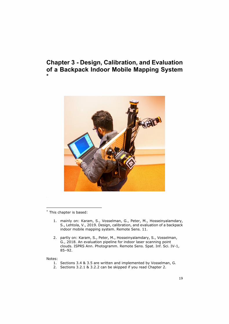
Chapter 3 - Design, Calibration, and Evaluation of a Backpack Indoor Mobile Mapping System *

1

* This chapter is based:

1. mainly on: Karam, S., Vosselman, G., Peter, M., Hosseinyalamdary, S., Lehtola, V., 2019. Design, calibration, and evaluation of a backpack indoor mobile mapping system. Remote Sens. 11.

2. partly on: Karam, S., Peter, M., Hosseinyalamdary, S., Vosselman, G., 2018. An evaluation pipeline for indoor laser scanning point clouds. ISPRS Ann. Photogramm. Remote Sens. Spat. Inf. Sci. IV-1, 85–92.

Notes: 1. Sections 3.4 & 3.5 are written and implemented by Vosselman, G. 2. Sections 3.2.1 & 3.2.2 can be skipped if you read Chapter 2.

Design, Calibration, and Evaluation of a Backpack Indoor Mobile Mapping System

20

Abstract Indoor mobile mapping systems are important for a wide range of applications starting from disaster management to straightforward indoor navigation. This chapter presents the design and performance of a low-cost backpack indoor mobile mapping system (ITC- Backpack) that utilizes a combination of laser range-finders (LRFs) to fully recover the 3D building model based on a feature-based SLAM algorithm. Specifically, we use robust planar features. These are advantageous, because oftentimes the final representation of the indoor environment is wanted in a planar form, and oftentimes the walls in an indoor environment physically have planar shapes. In order to understand the potential accuracy of our indoor models and to assess the system’s ability to capture the geometry of indoor environments, we develop novel evaluation techniques. In contrast to the state-of-the-art evaluation methods that rely on ground truth data, our evaluation methods can check the internal consistency of the reconstructed map in the absence of any ground truth data. Additionally, the external consistency can be verified with the often available as-planned state map of the building. The results demonstrate that our backpack system can capture the geometry of the test areas with angle errors typically below 1.5˚ and errors in wall thickness around 1 cm. An optimal configuration for the sensors is determined through a set of experiments that makes use of the developed evaluation techniques.

Chapter 3

21

3.1 Introduction Accurate measurement and representation of indoor environments has obtained a great scientific interest because of a multitude of potential applications (Biber et al., 2004; Borrmann et al.; 2008; Henry et al., 2014, Lehtola et al., 2017) such as disaster management, facility management, and indoor navigation. In particular, the use of indoor mobile mapping systems (IMMS) has shown promise in indoor data collection. Indoor spaces are satellite-denied environments, so it is an obvious choice to map them using relative positioning techniques, i.e., simultaneous localization and mapping (SLAM). A typical IMMS utilizes multiple sensors, e.g., laser scanners, inertial measurement units (IMU) and/or cameras, to capture the indoor environment. The sensors are attached onto a mobile platform that can be a pushcart, a robot, or human-carriable equipment (Blaser et al., 2018; Bosse et al., 2012; Trimble TIMMS1; Viametris iMS3D2; Wen et al., 2016). Laser scanners are used to measure the geometry, cameras are used to measure the texturing, and IMUs are used to estimate the changes in orientation of the scanner for SLAM purposes. The reason behind this use of the sensors is that RGB camera-based visual SLAM algorithms are extremely sensitive to lighting conditions, and fail in textureless spots, which are common in indoor environments. In turn, depth cameras (or RGB-D cameras) employed to alleviate for this shortcoming have a very short range, which is insufficient for large indoor spaces. Multiple human-carriable systems that employ laser scanners have been developed (Blaser et al., 2018; Chen et al., 2010; Lehtola et al., 2016; Naikal et al., 2009). This is not surprising, as easily carriable equipment is widely applicable. E.g., unlike pushcarts, it can be taken up and down the stairs, and because laser scanners are widely used sensors in capturing indoor geometry (Otero et al., 2020) as discussed earlier. This group of mobile mapping systems is further divided into hand-held and backpack systems. Lehtola et al. (2017) identify the state-of-the-art of these types. For hand-held commercial systems, Kaarta Stencil3 and ZEB1 REVO4 arguably present the current best in the market. For backpack systems, there are Leica Pegasus backpack5 and Gexcel Heron6. The IMMS implementations are quite different from each other. This is because when using relative positioning, the physical scanner platform and the

1 www.trimble.com 2 www.viametris.com 3 www.kaarta.com 4 www.geoslam.com 5 www.leica-geosystems.com 6 www.gexcel.it

Design, Calibration, and Evaluation of a Backpack Indoor Mobile Mapping System

22

employed data association method are intertwined. Therefore, advances oftentimes cannot be and are not incremental, since changing the hardware has an impact on the software and vice versa, and it can sometimes be advantageous if both the hardware and the software are re-designed. In this chapter, therefore, we introduce the design and the performance of our triple-2D-LRF (laser range finder) backpack system that is capable of outputting 3D indoor models from a 6 degree-of-freedom (6DOF) trajectory. Notably, this work differs from the previous triple-2D-LRF configuration state-of-the-art (Chen et al., 2010; Liu et al., 2010; Naikal et al. 2009) by employing two LRFs in slanted angles. Using slanted angles appears as a minor detail but turns out to be a quite fundamental. Specifically, it allows for combining the scan lines from the three 2D LRFs to form a quasi-3D point subset in the local platform coordinates that can then be robustly matched against a planar feature in the world coordinates. In other words, slanting the LRFs enables the use of robust planar features for SLAM-based data association and measurements of all three LRFs are used simultaneously for an integral estimation of the backpack pose, planes, calibration and relative sensor orientations. Investigating the use of planar features is advantageous for two reasons. First, oftentimes the final representation of the indoor environment is wanted in a planar form and formulating the use of planes already into the SLAM-algorithm is therefore motivated. Second, a typical wall in an indoor environment physically has a planar shape. As a second contribution, we present alternative evaluation techniques for assessing the performance of IMMSs. The proposed evaluation techniques estimate the reconstruction accuracy and quality even in the absence of a ground truth model. Here, in contrast to previous works (Lehtola et al., 2017; Liu et al., 2010; Maboudi et al., 2017, 2018; Thomson et al., 2013; Tran et al., 2019) that employ 3D ground truth data, the proposed methods uses 2D information in form of architectural constraints, i.e., the perpendicularity and parallelism of walls, or if available, floor plans. Furthermore, the proposed evaluation methods are utilized to find practical optima for the slanted LRFs angles. This chapter is organized as follows. Section 3.2 presents an overview of the previously developed human-carriable IMMSs and the state-of-the-art for evaluation methods on generated maps. Section 3.3 describes the design of our backpack system and the planar-feature SLAM method, based on the earlier works in (Karam et al., 2018) and (Vosselman, 2014). The calibration process of the mounted LRF is explained in Section 3.4. We elaborate the strategy of the registration process for LRFs in Section 3.5. We also present the proposed techniques to evaluate the system performance in Section 3.6, as partly introduced in (Karam et al., 2018). In Section 3.7, we show all

Chapter 3

23

implemented experiments that lead to the optimal configuration of the system. Section 3.8 is the conclusion.

3.2 Related Work Human-carriable systems can be divided into two categories: hand-held systems and backpack systems. After discussing the literature on these, we shall outline the literate on evaluation methods.

3.2.1 Hand-Held Systems Hand-held systems offer more flexibility because theoretically anywhere the operator can walk, the system can map. Examples of hand-held systems include ZEB1 from 3D Laser Mapping/CSIRO and Viametris1 iMS2D. ZEB1 consists of a laser range-finder (Hokuyo2 UTM-30LX with 30m range) and an inertial measurement unit (IMU, a MicroStrain 3DM-GX2) mounted on a passive linkage mechanism (Bosse et al., 2012). The system is based on the 6DOF SLAM algorithm that was developed to work with the capricious movement of the sensor. To operate ZEB1, it must be gently oscillated back and forth by the operator with a connection to the IMU to provide a solution. In comparison with other IMMS systems, ZEB1 has accessibility characteristics that allows it to map most of the areas in indoor environments, including stairwells. On the other hand, the performance of the device is acceptable only under specific conditions. For example, ZEB1 is not suitable for some environments in which the motion is not observable because the areas are featureless, large or open. Furthermore, the proposed SLAM algorithm will struggle if the oscillation of the sensor head stops for more than a few seconds. In the recent years, GeoSLAM3 has developed the mobile kinematic laser scanner ZEB-REVO as a commercial system for the measurement and mapping of multi-level 3D environments. It is also handheld, but the LRF is rotated on a fixed pole instead of irregular motion on a spring. iMS2D is a handheld scanner released by Viametris in 2016 for 2D indoor scanning. It comprises simply a 2D Hokuyo laser range-finder and fisheye camera. Another commercial hand-held system is Kaarta Stencil4 that is based on scientific work (Zhang et al., 2017). Stencil exploits LIDAR and IMU sensors for localization.

1 www.viametris.com 2 www.hokuyo.com 3 www.geoslam.com 4 www.kaarta.com

Design, Calibration, and Evaluation of a Backpack Indoor Mobile Mapping System

24

3.2.2 Backpack Mapping Systems These are instruments that are carried by a human operator. The key characteristic of this kind of system is that they have a non-zero pitch and roll. Naikal et al. (2009) mounted three LRFs (Hokuyo URG-04LX) orthogonally to each other together with a camera on a backpack platform. They aim to retrieve 6DOF localization in 3D space by integrating two processes. In the first, the transformation is estimated by applying the visual odometry technique and in the second, the rotation angles are estimated from the three scanners by applying the scan-matching algorithm. In later work by the same group, (Chen et al., 2010) added one more 2D scanner and two IMUs (HG9900 and InterSense) to the backpack system. The overall goal of their work was to estimate the trajectory the system follows during mapping. To achieve this goal, they developed four algorithms, which depend mainly on scan-matching, to retrieve the 6DOF pose translation of the system over time. The proposed framework is quite similar to that of the 6DOF scan-matching process in the SLAM approach of (Borrmann et al., 2008). The proposed algorithms have tradeoffs in terms of performance depending on the environment. For instance, algorithms that rely on planar floor assumptions provide more precise results only in the case of planar floor availability in the captured area. In addition, the algorithms lack a systematic filter that optimally combines the sensors’ measurements, such as a Kalman filter. In other work by the same group, Liu et al. (2010) replaced the yaw scanner (Hokuyo URG-04LX) by the Hokuyo UTM-30LX and added three cameras to the backpack platform. They used the previously developed algorithms (Chen et al., 2010) to estimate the system’s trajectory based on integrating the laser and IMU data. Each of the sensors is used independently to estimate one or more parameters of the system’s pose (x, y, z, roll, pitch, yaw) over time. E.g., the z value is estimated from the pitch scanner while x, y, and yaw values are estimated from the yaw scanner. The remaining pose parameters, namely roll and pitch, are estimated using the InterSense IMU. Since the camera is approximately synchronized with the scanners, Liu et al. estimate the pose of each image by nearest-neighbor interpolation of the pose parameters in order to texture the 3D model. Since the sensor rotation is determined independently for each of the three axes and not in an integrated manner, they need to assume that each scanner keeps scanning in the same plane over time, but that is unrealistic because of human operator motion. Therefore, this assumption will reflect negatively on the accuracy in the case of backpack rotation.

Chapter 3

25

Kim, (2013) presented an approach for 3D positioning of a previously developed backpack system (Naikal et al., 2009) in an indoor environment. The system consists of five LRFs (Hokuyo UTM-30LX), two IMUs (HG9900 and InterSense) and two fisheye cameras (GRAS-14S5C). In contrast to the other approaches, which use all the data, Kim’s approach identifies and incorporates the most credible data from each range finder. For localizing the system in an indoor environment, the cumulative shifts of the system over time are computed from yaw and pitch range finders using scan-matching techniques. Next, the point cloud is generated from roll range finders, restructured using a plane reconstruction algorithm, and textured using captured images. To avoid an expected misalignment in the case of the complex indoor environment, two 2D SLAM algorithms are proposed and integrated. The first one is to localize the system in the z-axis direction, and the second one for xy localization. The role of orientation sensor (InterSense IMU) is to measure roll and pitch angles to correct the measurements of the pitch and roll scanners and thus increase the accuracy of the scanner-based localization method. Only data from the roll scanner is used to generate the point cloud, while the pitch and yaw scanners will be responsible for 3D localization. In contrast to the yaw scanner, which scans in a plane parallel to the floor and helps to determine the xy location, a pitch scanner scans in a plane perpendicular to the floor and provides the third dimension (z) of the location. Thus, the localization algorithm may fail in case of discontinuities between consecutive walls or transparent objects, such as windows. Wen et al., (2016) developed an indoor backpack mobile mapping system consisting of three 2D LRFs (Hokuyo UTM-30LX) and an IMU (Xsens MTi-10). The system configuration consists of one LRF mounted horizontally while the other two are vertical. A 2D map of the building is constructed by a 2D SLAM using data from the horizontal range finder and then applying the rotations captured by the IMU to obtain a 3D pose of the system and thus a 3D map of the building. At the same time, the two vertical LRFs are responsible for creating 3D point clouds. Filgueira et al. (2016) presented a backpack mapping system constructed from a 3D LIDAR and an IMU for indoor data acquisition. The LIDAR is Velodyne VLP-16 that provides 360˚ horizontal and 30˚ vertical field of view. The SLAM algorithm utilizes the combination of two algorithms proposed in (Zhang & Singh, 2014) for indoor and outdoor positioning and mapping adapted for handling Velodyne’s data. They used the iterative closest point algorithm (ICP) for data association. The system was tested using the Faro Focus 3D scanner as a ground truth in two indoor environments with different characteristics. In later work by the same group, Lagüela et al. (2018) made some adjustments in the design of the system such as increasing the height of the scanner to avoid the occlusions that might occur because of the operator’s body.

Design, Calibration, and Evaluation of a Backpack Indoor Mobile Mapping System

26

Moreover, they mounted two webcams in the system for inspection purposes. In order to analyze the performance of the recent version of their backpack system, they did a comparison not only with the static scanner (Faro Focus 3D) as before, but also with the ZEB-REVO scanner. Blaser et al. (2018) proposed a wearable indoor mapping platform (BIMAGE) to provide 3D image-based data for indoor infrastructure management. The platform is mounted by a panoramic camera (FLIR Ladybug5), IMU and two Velodyne VLP-16 scanners (horizontal, vertical). A subsequent camera-based georeferencing was used to improve the camera positions provided by LIDAR SLAM.

3.2.3 Evaluation Methods Various evaluation strategies have been proposed to investigate the performance of the state-of-the-art IMMSs and quantify the quality of resulting point clouds. The most common strategy is a point cloud to point cloud (pc2pc or C2C) comparison after registering both clouds to the ground truth coordinate system, typically using CloudCompare software (Sirmacek et al., 2016; Thomson et al., 2013; Wen et al., 2016). While Thomson et al. (2013) investigated the earlier Viametris i-MMS and ZEB1 systems using TLS (Faro Focus3D) as ground truth, Maboudi et al. (2017) tested the later generations of Zebedee and Viametris (iMS3D and ZEB-Revo) using TLS (Leica P20) as ground truth. In addition to the pc2pc comparison, they compared the building information model’s (BIM) geometry derived from the tested systems to that derived from TLS. In later work (Maboudi et al., 2018), three additional analyses are proposed, namely points-to-planes distance, target-to-target distance and model-based evaluation. In a broader assessment process, Lehtola et al. (2017) proposed metrics to evaluate the full point cloud of eight state-of-the-art IMMSs against the point cloud of two TLSs (Leica P40, Faro Focus3D). Tran et al. (2019) provided comparison metrics for the evaluation of 3D planar representations of indoor environments. Specifically, if a 3D planar reference model is given, the completeness, correctness, and accuracy of the obtained model can be estimated against it. 3.3 Backpack System ITC-Backpack 3.3.1 System Description Due to the limited use and problems experienced by the previous indoor mapping systems, we developed our own indoor mobile mapping system shown in Figure 3.1. Our aim is to combine the proven performance of 2D SLAM-based trajectory estimates of push-cart systems with the flexibility of 3D hand-held or backpack systems. The system design has been proposed in (Vosselman, 2014) and is now implemented, optimised, calibrated, and

Chapter 3

27

evaluated. This backpack system consists of three LRFs (Hokuyo UTM-30LX), which are all utilized for a 3D (6 DOF) SLAM. In contrast to available 3D laser scanners, we try to keep the system design less expensive by only making use of these simple LRFs. The ranging noise according to our LRF’s specifications is ±30mm for [0.1 10]m range and ±50mm for [10 30]m range. This gives the Hokuyo UTM-30LX a key advantage over the range camera (Kinect) in capturing data inside large buildings such as airports where the dimensions of interior areas usually exceed 10 m. The top LRF (here referred to as 𝑆𝑆0) is mounted on the top of backpack system and it is approximately horizontal while the other two LRFs (𝑆𝑆1, 𝑆𝑆2) are mounted to the right and left of the 𝑆𝑆0 and are rotated around the moving direction (as in the i-MMS) as well as around the operator’s shoulder axis. These two rotation axes are perpendicular to each other as shown in Figure 3.1. To find the optimal values for the rotation angles, we conducted experiments that will be described in Section 3.7. There are two objectives for the rotation of the range finders: First, scanner configuration is purposed to cover surfaces perpendicular to the moving direction e.g., walls both behind and in front of the system, and second, it should allow for the association of points on new scan lines to previously seen walls. In case the scan lines would intersect walls vertically, this is not guaranteed when walking around corners or through doors. The field of view of the LRFs is limited to 270˚, and accordingly, there will be a 90˚ gap in each scanline. In order to cover all walls as good as possible, the two range finders (𝑆𝑆1, 𝑆𝑆2) are rotated around their axes such that their gaps (shadow areas) are directed towards the floor and the ceiling, respectively (Vosselman, 2014). A laptop running Ubuntu 16.04.X and the robot operation system (ROS) is used to communicate with all mounted sensors during data capture.

3.3.2 Coordinate Systems The proposed mapping system is a multi-sensor system and each one of the three mounted sensors has its own coordinate system. Next to the aforementioned sensor’s coordinate system, there are two additional coordinate systems: the frame (backpack) and model (local world) coordinate system.

Design, Calibration, and Evaluation of a Backpack Indoor Mobile Mapping System

28

Figure 3.1. The laptop used and the backpack system mounted by three LRFs 𝑆𝑆0(Top), 𝑆𝑆1(left), and 𝑆𝑆2(right) fitted with markers.

To integrate the data of the three LRF sensors, coordinates in their individual coordinate systems must be transformed into a unified coordinate system, which is termed the “frame coordinate system (f)”. We adopt the sensor coordinate system of 𝑆𝑆0 as the frame coordinate system. Assuming all sensors are rigidly mounted on the frame, the sensor coordinate systems of 𝑆𝑆1 and 𝑆𝑆2 are registered in this frame coordinate system using six transformation parameters, namely three rotation parameters (ω𝑠𝑠𝑖𝑖 ,ϕ𝑠𝑠𝑖𝑖 , κ𝑠𝑠𝑖𝑖) and three

translation parameters (𝑑𝑑𝑑𝑑𝑠𝑠𝑖𝑖 ,𝑑𝑑𝑑𝑑𝑠𝑠𝑖𝑖 ,𝑑𝑑𝑑𝑑𝑠𝑠𝑖𝑖). These parameters are determined in the registration process described in Section 3.5. Since the frame coordinate system is attached to a moving backpack system, a fixed coordinate system should be defined as a reference and a space in which the final indoor model will be described. This fixed coordinate system is termed the “model coordinate system (m)”. This model coordinate system is assumed to be the frame coordinate system at the start point of the trajectory. As long as the frame coordinate system is moving in 3D space, it is registered in the model coordinate system using six transformation parameters over time (t), namely three rotation parameters (ω𝑓𝑓(𝑡𝑡),ϕ𝑓𝑓(𝑡𝑡), κ𝑓𝑓(𝑡𝑡)) and three translation parameters (𝑑𝑑𝑑𝑑𝑓𝑓(𝑡𝑡),𝑑𝑑𝑑𝑑𝑓𝑓(𝑡𝑡),𝑑𝑑𝑑𝑑𝑓𝑓(𝑡𝑡)). Those changing parameters originate from the 6DOF SLAM algorithm explained to more detail in the next section.

Chapter 3

29

3.3.3 6DOF SLAM We defined a feature-based SLAM algorithm in which the range observations of all three scanners contribute to the integral estimation of all six pose parameters. Starting point for the SLAM is the association of newly measured points to already estimated planes in the indoor environment. The six pose parameters are modeled as a function over time using B-splines. The planes are simply defined by a normal vector (𝑛𝑛) and distance to the origin (𝑑𝑑) in the model coordinate system. For a point 𝑑𝑑𝑚𝑚 in the model coordinate system it should therefore hold:

𝑛𝑛𝑑𝑑𝑚𝑚 − 𝑑𝑑 = 0, (3.1)

As the laser scanners after registration provide point coordinates 𝑑𝑑𝑓𝑓 in the frame coordinate system, we write 𝑑𝑑𝑚𝑚 = 𝑅𝑅(𝑡𝑡) 𝑑𝑑𝑓𝑓 + 𝑣𝑣(𝑡𝑡) to transform a point 𝑑𝑑𝑓𝑓 in the frame coordinate system to point 𝑑𝑑𝑚𝑚 in the model coordinate system by a rotation 𝑅𝑅(𝑡𝑡) and a translation 𝑣𝑣(𝑡𝑡). Substituting 𝑑𝑑𝑚𝑚 in Eq. (3.1) provides the observation equation

𝐸𝐸{𝑛𝑛�𝑅𝑅(𝑡𝑡)𝑑𝑑𝑓𝑓 + 𝑣𝑣(𝑡𝑡)� − 𝑑𝑑} = 0, (3.2)

The trajectory of the frame, as well as the rotations, are modelled by B-splines as a function of time (𝑡𝑡). For instance, roll ω is formulated as follow:

𝜔𝜔(𝑡𝑡) = ∑ 𝛼𝛼𝜔𝜔,𝑖𝑖 .𝐵𝐵𝑖𝑖(𝑡𝑡)𝑖𝑖 , (3.3)

where 𝛼𝛼𝜔𝜔,𝑖𝑖 is the spline coefficient for 𝜔𝜔 to be estimated on interval 𝑖𝑖. The model coordinate system is defined based on the first scans of the three scanners. Since there is no information about the system speed yet, the rotation and translation defined during establishing the model coordinate system are used to predict the orientation and translation of the system over the time interval of the first two scanlines using a constant local spline. Later, more data will be captured by the LRFs. Then, for pose parameters prediction, the local spline estimation is implemented using the data of only three to four scanlines of each of the laser scanners. The locally estimated splines are linearly extrapolated to obtain a prediction of the frame pose over the time interval of the next scanline acquisition. After segmenting the next scanline using a line segmentation procedure (Peter et al., 2017), a test on a distance threshold is used to decide whether a

Design, Calibration, and Evaluation of a Backpack Indoor Mobile Mapping System

30

segment should be associated to an already reconstructed plane or be used to instantiate a new plane need. Currently, only horizontal and vertical planes are used. After setting up the corresponding observation equations the pose parameters are estimated for the next time interval. After processing the whole dataset with locally defined spline functions, one integral adjustment estimates spline coefficients for the whole trajectory as well as all parameters of planes in the model coordinate system.

3.4 Calibration Process In this research the term “calibration” refers to the estimation of biases in the raw range data acquired by every single LRF, in our case the Hokuyo UTM-30LX. The calibration of the laser range finders is needed to optimise the quality of the reconstructed point cloud.

3.4.1 Calibration Facility For carrying out the calibration process, a classroom in ITC faculty building was selected as a calibration facility. The room has an almost rectangular shape with white walls and is of a suitable size. The reference data was captured by tape measurements. 3.4.2 Calibration Eq. (3.4) formulates the relationship between the coordinates in the LRF sensor system (𝑑𝑑𝑠𝑠 ,𝑑𝑑𝑠𝑠), and the model system (𝑑𝑑𝑚𝑚,𝑑𝑑𝑚𝑚), and Eq. (3.5) describes the known location of a wall in the model system (distance 𝑑𝑑, orientation 𝜃𝜃). All relationships are in 2D as we assume the LRF to be scanning perpendicular to the walls.

�𝑑𝑑𝑚𝑚𝑑𝑑𝑚𝑚� = � 𝑐𝑐𝑐𝑐𝑐𝑐 𝛽𝛽 𝑐𝑐𝑖𝑖𝑛𝑛 𝛽𝛽

−𝑐𝑐𝑖𝑖𝑛𝑛 𝛽𝛽 𝑐𝑐𝑐𝑐𝑐𝑐 𝛽𝛽� �𝑑𝑑𝑠𝑠𝑑𝑑𝑠𝑠� + �𝑑𝑑0𝑑𝑑0

�, (3.4)

𝑑𝑑𝑚𝑚 ∗ 𝑐𝑐𝑐𝑐𝑐𝑐 𝜃𝜃 + 𝑑𝑑𝑚𝑚 ∗ 𝑐𝑐𝑖𝑖𝑛𝑛 𝜃𝜃 − 𝑑𝑑 = 0, (3.5)

where 𝛽𝛽 is the rotation of the LRF, and (𝑑𝑑0,𝑑𝑑0) represent the location of the LRF in the local model coordinate system. Each indoor environment is decorated differently, and the surface materials are different, e.g., on walls. The surface material properties, e.g., color, brightness, and smoothness, each impact the range measurements to a small degree (Park et al., 2010). This change in surface properties to the range

Chapter 3

31

measurements is compensated with the calibration of Eq. (3.6). In our calibration model we use a scale factor (𝜆𝜆𝑟𝑟) and offset (Δ𝑟𝑟) for the range measurements as well as a scale factor (𝜆𝜆𝛼𝛼) for the scanning direction. The coordinates in LRF sensor system are obtained from the observed polar coordinates (range 𝑟𝑟, scanning direction 𝛼𝛼).

�̂�𝑟 = 𝜆𝜆𝑟𝑟𝑟𝑟 + Δ𝑟𝑟, (3.6)

�𝑑𝑑𝑠𝑠𝑑𝑑𝑠𝑠� = � 𝑐𝑐𝑐𝑐𝑐𝑐 𝜆𝜆𝛼𝛼𝛼𝛼 𝑐𝑐𝑖𝑖𝑛𝑛 𝜆𝜆𝛼𝛼𝛼𝛼

−𝑐𝑐𝑖𝑖𝑛𝑛 𝜆𝜆𝛼𝛼𝛼𝛼 𝑐𝑐𝑐𝑐𝑐𝑐 𝜆𝜆𝛼𝛼𝛼𝛼� ��̂�𝑟0�, (3.7)

Equations 3.4-3.7 are combined to obtain a single equation with the pose of the LRF (𝑑𝑑0, 𝑑𝑑0, 𝛽𝛽) and the calibration parameters (𝜆𝜆𝑟𝑟, Δ𝑟𝑟, 𝜆𝜆𝛼𝛼) as the unknown parameters. The LRF to be calibrated is put on different locations in the calibration room with different rotations to optimise the estimability of the calibration parameters. After a warming up period, the data of a few scan lines per pose are used to estimate all pose and calibration parameters. Points of those scan lines were manually labelled with the index number of the corresponding wall. Estimated range offsets and range scale factors were typically below 4 cm and 0.8% respectively, whereas the estimated angle scale error was usually below 0.7%. After calibration the remaining residuals between the points and the wall planes show a root mean square value below 1 cm. This is clearly better than the noise level specified by the manufacturer (3 cm). 3.4.3 Self-Calibrations Similar to self-calibration in the photogrammetric bundle adjustment, it is feasible to include the estimation of the sensor calibration parameters of all three LRFs in the SLAM process. In absence of a reference (tape) measurement in the SLAM procedure, we can, however, not estimate the range scale factors of all LRFs as the scale of the resulting point cloud would then be undetermined. Hence, we fix the range scale of the top LRF (𝑆𝑆0) to the value obtained in the calibration room and include the remaining eight calibration parameters as additional unknowns to the SLAM equations. 3.5 Relative Sensor Registration To accurately fuse data from the three LRF sensors, their coordinate systems must be registered to a common reference system. This requires the estimation of the relative pose of the LRFs with respect to each other. We adopt the sensor coordinate system of the horizontal LRF as the backpack frame coordinate system and register as accurately as possible the two slanted LRFs with respect to this system. The registration is performed in two steps: marker registration and fine registration. These processes do not require a room with known

Design, Calibration, and Evaluation of a Backpack Indoor Mobile Mapping System

32

dimensions, but the data should be captured in a specific way as described in the following two paragraphs. 3.5.1 Initial Registration The registration method is based on 3D tracking technology for markers (see Figure 3.1) attached to the heads of the mounted LRFs to achieve an approximate registration. We make use of the ‘ar_track_alvar’ package1, which is a robot operation system (ROS) wrapper for Alvar, an open source library for virtual and augmented reality (AR) marker tracking. As the laptop’s webcam is involved in the registration process, it also needs to be calibrated using another ROS package. As the rotation and translation between the markers and the LRF sensor coordinate systems can be determined to a few mm and degree, the relative marker positions estimated with the ROS package can be used to infer approximate values for the parameters of the relative registration of the three LRFs. 3.5.2 Fine Registration The goal of this process is to refine the approximate values for the registration parameters obtained during the previous approach and assumed to be acceptably accurate. This fine registration imposes two constraints on the captured sensor data. As the indoor environment usually contains large planes, the first constraint used is co-planarity of three line segments on the same plane simultaneously scanned by the three LRFs (Choi et al., 2014; Fernández-Moral et al., 2015). The second constraint is inferred from the perpendicularity of two observed planes (Choi et al., 2014). The data collection is carried out with the backpack (ITC-Backpack) on the back of the operator. In order to estimate all registration parameters, the planar surfaces should be observed by the backpack system with different orientations. Therefore, first the operator stands inside a suitable area, in which the previous constraints are applicable, and starts capturing data while bending forward and sideward (right and left). Then, the operator rotates by 90˚ and bends again in the same way. These rotation and bending steps are repeated until the operator is back at the initial orientation. The captured data pass through a series of processing steps before being subject to the registration’s constraints. Firstly, the scanlines from each LRF are segmented by a line segmentation algorithm (Peter et al., 2017) and

1 http://wiki.ros.org/ar_track_alvar

Chapter 3

33

transformed to a frame system using the approximated parameters. Next, all the pairs of nearly co-planar line segments captured by two different LRFs are collected. To define the aforementioned constraints, two types of observation equations are formulated, namely perpendicularity and coplanarity. Let’s denote 𝑙𝑙𝑗𝑗𝑖𝑖 as the direction vector of a segment, where i refers to a plane (A, B) and j refers to one of the LRFs (0, 1, 2). The relative transformations of 𝑆𝑆1and 𝑆𝑆2 with respect to 𝑆𝑆0 are described by 12 parameters, a 3D rotation (𝑅𝑅1(𝜔𝜔1,𝜙𝜙1, 𝜅𝜅1) and 𝑅𝑅2(𝜔𝜔2,𝜙𝜙2,𝜅𝜅2)) and a 3D translation (𝑇𝑇1 and 𝑇𝑇2) for each. If two planes A and B are perpendicular it will hold that:

(𝑙𝑙0𝐴𝐴 × 𝑅𝑅1𝑙𝑙1𝐴𝐴) ∙ (𝑙𝑙0𝐵𝐵 × 𝑅𝑅1𝑙𝑙1𝐵𝐵) = 0, (3.8) where: 𝑙𝑙0𝐴𝐴 × 𝑅𝑅1𝑙𝑙1𝐴𝐴 is the normal vector of plane A expressed in the coordinate system of 𝑆𝑆0, and 𝑙𝑙0𝐵𝐵 × 𝑅𝑅1𝑙𝑙1𝐵𝐵 is the normal vector of plane B expressed in the coordinate system of 𝑆𝑆0. The unknowns in this equation are the rotation angles of 𝑆𝑆1 in 𝑅𝑅1. In a common coordinate system, the two direction vectors of the line segments as well as the vector connecting the midpoints (𝑝𝑝0𝑖𝑖 , 𝑝𝑝1𝑖𝑖 , 𝑝𝑝2𝑖𝑖 ) must be coplanar. Taking the coordinate system of 𝑆𝑆0, the coplanarity equation for plane A can be formulated as follows:

(𝑙𝑙0𝐴𝐴 × 𝑅𝑅1𝑙𝑙1𝐴𝐴) ∙ (𝑝𝑝0𝐴𝐴 − 𝑅𝑅1𝑝𝑝1𝐴𝐴 − 𝑇𝑇1) = 0, (3.9) As three-line segments could be recorded with three different LRFs in each of three perpendicular planes already the data captured at a single pose of the mapping system would yield nine independent coplanarity equations and three independent perpendicularity equations. Thus, this would already provide sufficient observations to estimate all 12 registration parameters. However, to increase the reliability of the estimation we use a much larger number of equations with data of different poses of the backpack captured according to the described bending procedure. The scanning frequency of the Hokuyo used is 40 HZ; therefore, after one minute, each LRF records 2400 scanlines thereby leading to a very large number of observation equations. Using the available approximated values from marker registration and after linearizing the formulated equations, an accurate estimate of the transformation parameters can be obtained by applying a least-squares estimation. The standard deviations of the estimated parameters are around 1 mm for the translations and around 0.05˚ for the rotation angles.

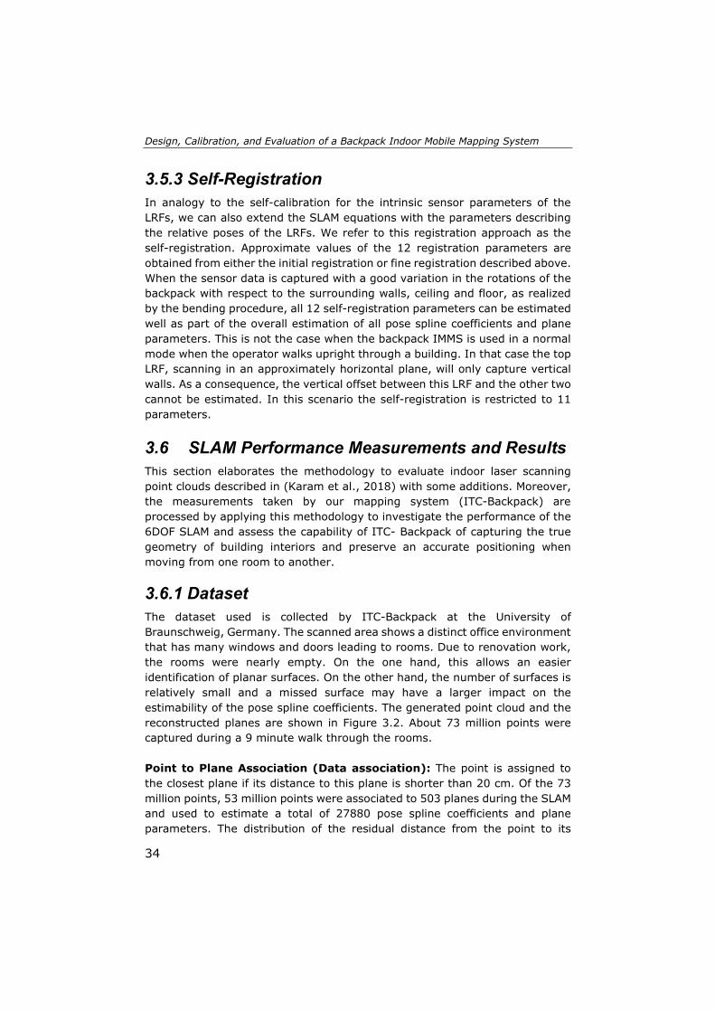
Design, Calibration, and Evaluation of a Backpack Indoor Mobile Mapping System

34

3.5.3 Self-Registration In analogy to the self-calibration for the intrinsic sensor parameters of the LRFs, we can also extend the SLAM equations with the parameters describing the relative poses of the LRFs. We refer to this registration approach as the self-registration. Approximate values of the 12 registration parameters are obtained from either the initial registration or fine registration described above. When the sensor data is captured with a good variation in the rotations of the backpack with respect to the surrounding walls, ceiling and floor, as realized by the bending procedure, all 12 self-registration parameters can be estimated well as part of the overall estimation of all pose spline coefficients and plane parameters. This is not the case when the backpack IMMS is used in a normal mode when the operator walks upright through a building. In that case the top LRF, scanning in an approximately horizontal plane, will only capture vertical walls. As a consequence, the vertical offset between this LRF and the other two cannot be estimated. In this scenario the self-registration is restricted to 11 parameters.

3.6 SLAM Performance Measurements and Results This section elaborates the methodology to evaluate indoor laser scanning point clouds described in (Karam et al., 2018) with some additions. Moreover, the measurements taken by our mapping system (ITC-Backpack) are processed by applying this methodology to investigate the performance of the 6DOF SLAM and assess the capability of ITC- Backpack of capturing the true geometry of building interiors and preserve an accurate positioning when moving from one room to another. 3.6.1 Dataset The dataset used is collected by ITC-Backpack at the University of Braunschweig, Germany. The scanned area shows a distinct office environment that has many windows and doors leading to rooms. Due to renovation work, the rooms were nearly empty. On the one hand, this allows an easier identification of planar surfaces. On the other hand, the number of surfaces is relatively small and a missed surface may have a larger impact on the estimability of the pose spline coefficients. The generated point cloud and the reconstructed planes are shown in Figure 3.2. About 73 million points were captured during a 9 minute walk through the rooms. Point to Plane Association (Data association): The point is assigned to the closest plane if its distance to this plane is shorter than 20 cm. Of the 73 million points, 53 million points were associated to 503 planes during the SLAM and used to estimate a total of 27880 pose spline coefficients and plane parameters. The distribution of the residual distance from the point to its

Chapter 3

35

associated plane is shown in Figure 3.2. 97% of the points have residuals below 3 cm and the RMS value of these residuals is only 1.3 cm. This means that the method is self-consistent. The RMS value, however, does not represent well the overall quality of the dataset. Further quality measures are therefore developed and used in the next section. Figure 3.3 shows a top view of the generated point cloud, where points are colored based on their respective residuals. The data association rule, which assigns points to planes, experiences problems, when two distinct planes are too close to each other. For example, a door that is wide open and thus close to the wall, or a door that is only slightly open and thus close to the other wall are typical causes for such behaviour. Moreover, there can be dynamic noise, for instance, if a door is opening while the data is being captured. Clear examples of both problematic cases are highlighted in Figure 3.3. The problem resulting from merging a door with a nearby wall, can be seen inside the orange dashed rectangle.

3.6.2 Evaluation Techniques As SLAM-based point clouds usually suffer from registration errors because of the dead-reckoning nature of SLAM algorithms, the performance of the mapping system and the accuracy of the provided results needs to be analyzed. While most current evaluation methods rely on the availability of reference data, we develop several techniques to investigate the mapping system in the absence of an accurate ground truth model. The proposed techniques take advantage of regularities in wall configurations to check how well the rooms are connected, and thus how well the environment is reconstructed. Since most buildings have a floor plan (though often outdated), we utilize that as an external information source to check the quality of the generated indoor model, but without relying on an accurate registration of the point cloud to the floor plan. We classify the developed techniques into three independent groups: (1) techniques using architectural constraints; (2) techniques using a floor plan; and (3) completeness techniques. To simplify the process and because the indoor environments mainly consists of planar and vertical structures, the first two groups make use of 2D edges derived from such structures. As our feature-based SLAM outputs both point clouds and 3D reconstructed planes, the 2D edges are derived from the projection of the vertical planes onto the XY-plane, as presented in (Karam et al., 2018). We address the third group of evaluation techniques in the study of the optimal sensor configuration described in Section 3.7.

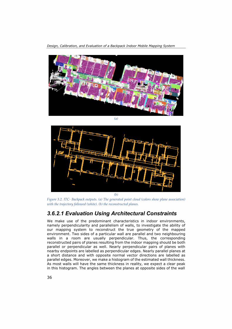
Design, Calibration, and Evaluation of a Backpack Indoor Mobile Mapping System

36

(a)

(b)

Figure 3.2. ITC- Backpack outputs. (a) The generated point cloud (colors show plane association) with the trajectory followed (white). (b) the reconstructed planes.

3.6.2.1 Evaluation Using Architectural Constraints We make use of the predominant characteristics in indoor environments, namely perpendicularity and parallelism of walls, to investigate the ability of our mapping system to reconstruct the true geometry of the mapped environment. Two sides of a particular wall are parallel and two neighbouring walls in a room are usually perpendicular. Thus, the corresponding reconstructed pairs of planes resulting from the indoor mapping should be both parallel or perpendicular as well. Nearly perpendicular pairs of planes with nearby endpoints are labelled as perpendicular edges. Nearly parallel planes at a short distance and with opposite normal vector directions are labelled as parallel edges. Moreover, we make a histogram of the estimated wall thickness. As most walls will have the same thickness in reality, we expect a clear peak in this histogram. The angles between the planes at opposite sides of the wall

Chapter 3

37

(a)

(b)

Figure 3.3. The residuals between the points and the estimated planes. (a) Frequency of the residuals with a logarithmic scale for the y-axis and a linear scale for the x-axis. (b) Top view of the generated point cloud. All white points have residuals below 3 cm and points with larger residuals are marked with either red or blue colour, depending on the sign. The orange dashed rectangle marks an example of a plane representing a door being merged with another plane, which represents a wall that is near the door. The orange dashed oval surrounds an opening door.

and the wall thickness histogram provide a good impression of the ability of the mapping system to maintain an accurate positioning when moving from a room to another. We assume two walls to be perpendicular when the angle between their 2D edges in the XY plane is between 85˚ and 95˚ and their end points, that are close to the intersection point and should represent the corner point, are within 30 cm. Furthermore, the angle between the parallel edges should be in the range [0˚ ±5˚] with the distance between them not exceeding 30 cm. The results of the plane pairing on the Braunschweig data are shown in Figure 3.4a-

0 0.02 0.04 0.06 0.08 0.1 0.12 0.14 0.16 0.18 0.2

Residuals[m]

10 2

10 3

10 4

10 5

10 6

10 7

10 8

Freq

uenc

y

97%

of p

oint

s

Design, Calibration, and Evaluation of a Backpack Indoor Mobile Mapping System

38

b. In addition, we compute the angle error as the deviation from the perfect parallelism (0˚) and perpendicularity (90˚) and build histograms of these errors as shown in Figure 3.4c-d. In reality walls are, of course, never constructed perfectly parallel or perpendicular to other walls, but the deviation from this is expected to be an order of magnitude smaller than the deviations observed in the reconstructed model. The results show that the angle between two sides of a wall is determined less accurately than that between two perpendicular planes in the same room. This is consistent with the expected performance of SLAM algorithms, as the two walls sides are not seen at the same point of time. Moreover, we note high percentages in the above histograms in bins where the angles deviate by more than 2.5˚ from their expected values of 0˚ and 90˚. By tracking the source of these high percentages, we found that they mainly originate from incorrectly reconstructed planes, such as open doors. In addition, the measurements of walls' thickness demonstrate that there are two standard types of walls in the building and the standard deviation of the thickness is around 1 cm. 3.6.2.2 Evaluation Using a Floor Plan Nowadays, many buildings have 2D floor plans reflecting the as-planned state from before construction. We investigate the feasibility of using a simple 2D floor plan in analyzing the accuracy of the reconstructed model. Transformation: As the 2D edges derived from our SLAM-based point clouds and those in the floor plan (see Figure 3.5) are in two different coordinate systems, we have to register them in the same coordinate system for valid comparison. We use a 2D similarity transform and estimate the transformation parameters based on a number of manually selected corresponding points. The main goal of this transformation is to identify correspondences between the edges extracted from the point cloud and those in the floor plan. We do not estimate residual distances or angles between an edge in the point cloud and an edge in the floor plan, because we want to keep the comparison process independent of the chosen coordinate systems and quality of the registration. Therefore, we only compare the angles and distances between edges or points extracted from the point cloud to the angles and distances between the corresponding edges or points in the floor plan. The left image in Figure 3.5 shows the digitized floor plan of the scanned floor.

Chapter 3

39

Figure 3.4. The results of the architectural constraints method. (a) all pairs of parallel edges. (b) all pairs of perpendicular edges. (c) Percentages of angle errors between parallel edges within the range [0˚ 5˚]. (d) Percentages of angle errors between parallel edges within the range [85˚ 95˚].

Figure 3.5. The digitized floor plan (left) and point cloud-based edges for Braunschweig data (right)

Edge Matching: When both sets of edges are registered in the same coordinate system, we start matching the corresponding edges. Firstly, we detect all point cloud-based edges that are expected to belong to a room in the floor plan using a buffer around the room polygon, termed a polygon-buffer. Secondly, we choose which of the detected edges most probably represents the side of a wall in that room using another buffer (30 cm width) around each of the room’s edges, termed an edge-buffer as well as the normal vector direction to avoid confusion with edges of the opposite side of the wall. In contrast to other objects, walls usually are the dominant uniform features present in buildings and as such provide possibility to reconstruct large and reliable plane features for the SLAM process. Therefore, a further selection based on height information is implemented to keep only edges that most probably belong to walls. We implement a filtering process room by room in

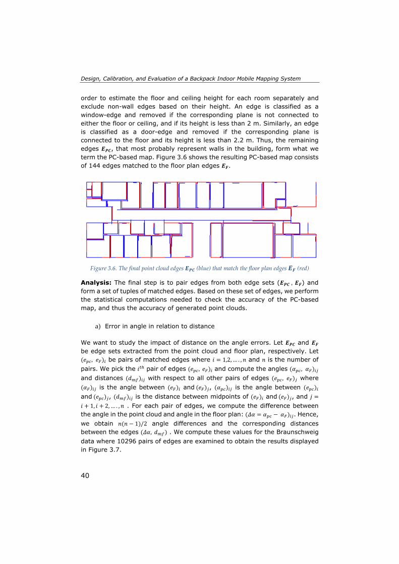
Design, Calibration, and Evaluation of a Backpack Indoor Mobile Mapping System

40

order to estimate the floor and ceiling height for each room separately and exclude non-wall edges based on their height. An edge is classified as a window-edge and removed if the corresponding plane is not connected to either the floor or ceiling, and if its height is less than 2 m. Similarly, an edge is classified as a door-edge and removed if the corresponding plane is connected to the floor and its height is less than 2.2 m. Thus, the remaining edges 𝑬𝑬𝑷𝑷𝑷𝑷, that most probably represent walls in the building, form what we term the PC-based map. Figure 3.6 shows the resulting PC-based map consists of 144 edges matched to the floor plan edges 𝑬𝑬𝑭𝑭.

Figure 3.6. The final point cloud edges 𝑬𝑬𝑷𝑷𝑷𝑷 (blue) that match the floor plan edges 𝑬𝑬𝑭𝑭 (red)

Analysis: The final step is to pair edges from both edge sets (𝑬𝑬𝑷𝑷𝑷𝑷 , 𝑬𝑬𝑭𝑭) and form a set of tuples of matched edges. Based on these set of edges, we perform the statistical computations needed to check the accuracy of the PC-based map, and thus the accuracy of generated point clouds.

a) Error in angle in relation to distance

We want to study the impact of distance on the angle errors. Let 𝑬𝑬𝑷𝑷𝑷𝑷 and 𝑬𝑬𝑭𝑭 be edge sets extracted from the point cloud and floor plan, respectively. Let (𝑒𝑒𝑝𝑝𝑝𝑝 , 𝑒𝑒𝐹𝐹)𝑖𝑖 be pairs of matched edges where 𝑖𝑖 = 1,2, … . ,𝑛𝑛 and 𝑛𝑛 is the number of pairs. We pick the 𝑖𝑖𝑡𝑡ℎ pair of edges (𝑒𝑒𝑝𝑝𝑝𝑝 , 𝑒𝑒𝐹𝐹)𝑖𝑖 and compute the angles (𝛼𝛼𝑝𝑝𝑝𝑝 , 𝛼𝛼𝐹𝐹)𝑖𝑖𝑗𝑗 and distances (𝑑𝑑𝑚𝑚𝑓𝑓)𝑖𝑖𝑗𝑗 with respect to all other pairs of edges (𝑒𝑒𝑝𝑝𝑝𝑝 , 𝑒𝑒𝐹𝐹)𝑗𝑗 where (𝛼𝛼𝐹𝐹)𝑖𝑖𝑗𝑗 is the angle between (𝑒𝑒𝐹𝐹)𝑖𝑖 and (𝑒𝑒𝐹𝐹)𝑗𝑗, (𝛼𝛼𝑝𝑝𝑝𝑝)𝑖𝑖𝑗𝑗 is the angle between (𝑒𝑒𝑝𝑝𝑝𝑝)𝑖𝑖 and (𝑒𝑒𝑝𝑝𝑝𝑝)𝑗𝑗, (𝑑𝑑𝑚𝑚𝑓𝑓)𝑖𝑖𝑗𝑗 is the distance between midpoints of (𝑒𝑒𝐹𝐹)𝑖𝑖 and (𝑒𝑒𝐹𝐹)𝑗𝑗, and 𝑗𝑗 =𝑖𝑖 + 1, 𝑖𝑖 + 2, … . ,𝑛𝑛 . For each pair of edges, we compute the difference between the angle in the point cloud and angle in the floor plan: (𝛥𝛥𝛼𝛼 = 𝛼𝛼𝑝𝑝𝑝𝑝 − 𝛼𝛼𝐹𝐹)𝑖𝑖𝑗𝑗. Hence, we obtain 𝑛𝑛(𝑛𝑛 − 1)/2 angle differences and the corresponding distances between the edges (𝛥𝛥𝛼𝛼, 𝑑𝑑𝑚𝑚𝑓𝑓) . We compute these values for the Braunschweig data where 10296 pairs of edges are examined to obtain the results displayed in Figure 3.7.

Chapter 3

41

The results presented in Figure 3.7a-b demonstrate that the errors in the angle between point cloud edges are small; approximately 81% are in the range [-1˚ 1˚]. The two noticeable small peaks in Figure 3.7b around ±3˚ refer to some larger errors, which may belong to only a few poorly reconstructed planes. Overall, as can be seen in Figure 3.7a, the distance between edges has no impact on the error in the angle between them. To identify the poorly estimated outlier edges, we construct Figure 3.8 in which all edge pairs that have an angle error of 3˚ or more are presented. The pattern in this figure clearly indicates which edges are mostly involved in edge pairs with large angle errors. We observed five outlier edges and excluded them from the computations in order to obtain a better picture of the potential quality of the system; see Figure 3.7c-d. Table 3.1 shows standard deviation values and the number of edge pairs that are involved in the computations for both cases, both before and after excluding outlier edges. We can see that the removal of the outlier edges leads to a 25% decrease in the estimated standard deviation.

(a)

(c)

(b)

(d)

Figure 3.7. (a) Errors in angle as relation of distance. (b) Histogram of the percentages of errors. (c) Errors in angle as relation of distance after excluding outlier edges. (d) Histogram of the percentages of errors after excluding outlier edges.

0 5 10 15 20 25 30 35 40 45 50

Dist[m]

-8

-6

-4

-2

0

2

4

6

8

d-al

pha[

deg]

-8 -6 -4 -2 0 2 4 6

d-alpha[deg]

0

5

10

15

Perc

enta

ge[%

]

-6 -4 -2 0 2 4 6

d-alpha[deg]

0

5

10

15

Perc

enta

ge[%

]

Design, Calibration, and Evaluation of a Backpack Indoor Mobile Mapping System

42

Figure 3.8. All edge pairs that have an angle error of 3˚ or more.

Table 3.1. Values of mean, standard deviation, and the number of edges pairs that are involved in the computations for both cases, before and after excluding outlier edges

Before After Mean 0.01˚ 0.00˚

Std Dev. 1.14˚ 0.85˚ Edge-Pairs Nr 10296 9591

Since the perpendicular and parallel edges are already labelled (Section 3.6.2), we also computed these values for each type of edge separately. We found that the error in angle over distance is not related to the attitude of one edge to other. Moreover, we investigated the impact of time on the angle errors as the 3D planes are reconstructed over time through applying the SLAM algorithm. However, the results show no relation between the time and angle errors. The reason for this is that the operator returned to the same corridor during the data capturing in Braunschweig, which in turn leads to frequent loop closures that prevent the errors from accumulating.

b) Error in distance in relation to distance

Besides the previous computations of angle errors based on the pairs of edges, we compute the distance errors based on pairs of edges’ end points. However, because the point cloud-based map is usually incomplete, we find corner points by intersecting the neighbouring edges. We utilize the topology of the floor plan and intersect edges from 𝑬𝑬𝑷𝑷𝑷𝑷 if their matched floor plan edges 𝑒𝑒𝐹𝐹 are connected. Let 𝑃𝑃𝑝𝑝𝑝𝑝 and 𝑃𝑃𝐹𝐹 be intersection points obtained from the floor plan and the point cloud, respectively. Let (𝑝𝑝𝑝𝑝𝑝𝑝 , 𝑝𝑝𝐹𝐹)𝑖𝑖 be pairs of points where 𝑖𝑖 = 1,2, … . ,𝑛𝑛 and 𝑛𝑛 is the number of pairs. We pick the 𝑖𝑖𝑡𝑡ℎ pair of points (𝑝𝑝𝑝𝑝𝑝𝑝 ,𝑝𝑝𝐹𝐹)𝑖𝑖 and compute the distances (𝑑𝑑𝑝𝑝𝑝𝑝 , 𝑑𝑑𝑓𝑓)𝑖𝑖𝑗𝑗 with respect to all other pairs of points (𝑝𝑝𝑝𝑝𝑝𝑝 , 𝑝𝑝𝐹𝐹)𝑗𝑗 where (𝑑𝑑𝑓𝑓)𝑖𝑖𝑗𝑗 is the distance between (𝑝𝑝𝐹𝐹)𝑖𝑖 and (𝑝𝑝𝐹𝐹)𝑗𝑗, (𝑑𝑑𝑝𝑝𝑝𝑝)𝑖𝑖𝑗𝑗 is the distance between (𝑝𝑝𝑝𝑝𝑝𝑝)𝑖𝑖 and (𝑝𝑝𝑝𝑝𝑝𝑝)𝑗𝑗 , and j= 𝑖𝑖 + 1, 𝑖𝑖 + 2, … ,𝑛𝑛. Next, the error in the distances (𝛥𝛥𝑑𝑑 = 𝑑𝑑𝑓𝑓 −

Chapter 3

43

𝑑𝑑𝑝𝑝𝑝𝑝)𝑖𝑖𝑗𝑗 will be plotted against the distances (𝑑𝑑𝑓𝑓)𝑖𝑖𝑗𝑗 to check if the error in distance depends on the distance between floor plan points. Computing the error in distance in this way will remove the systematic error that would otherwise result from errors in the transformation. From the data used, we obtain 128 corner points leading to 8128 pairs of points involved in the distance errors computation as a function of distance. Figure 3.9 shows that the errors in distance are sometimes quite large (~40 cm). The source for such an error is not necessarily the mapping system or the proposed SLAM algorithm, but it could be also the outdated floor plan used. We noted some differences in the width of some walls between the floor plan and the realised construction.

Figure 3.9. Errors in distance in relation to the distance (left) and Histogram of the percentages of errors (right).

We carried out an analysis similar to that shown in Figure 3.8 to identify the poorly reconstructed corners (outlier points) using the distance between 𝑝𝑝𝑝𝑝𝑝𝑝 and 𝑝𝑝𝐹𝐹. The comparison of the results before and after excluding these outlier points does not show a significant improvement. However, it is not possible to draw the conclusion whether these errors are caused by the ground truth model used or the mapping system. 3.7 Determining Optimal Configuration As our system is equipped with several sensors, we utilize the proposed evaluation techniques in the previous section to find the optimal configuration. 3.7.1 Studied Configurations It is important to avoid occlusion in the data and to acquire sufficient geometrical information of the building to be mapped. As our mapping system is composed of three 2D sensors, we seek for the optimal mounting

0 5 10 15 20 25 30 35 40 45 50

Dist[m]

-0.6

-0.4

-0.2

0

0.2

0.4

0.6

0.8

d-D[

m]

-1 -0.8 -0.6 -0.4 -0.2 0 0.2 0.4 0.6 0.8 1

d-D[m]

0

2

4

6

8

10

12

14

16

18

Perc

enta

ge[%

]

Design, Calibration, and Evaluation of a Backpack Indoor Mobile Mapping System

44

configuration of these sensors (LRFs) on the backpack by making use of the proposed evaluation methods above in Section 3.6.2. The optimal sensor configuration is defined through an experimental comparison of different configurations. The experiments were conducted in an indoor office environment at our university. The three selected rooms, with a corridor in-between, were captured by the system for several possible configurations. A set of criteria was used to select the experimented configurations. In order to see all the walls around the system, 𝑆𝑆0 is always be horizontal and above the operator’s head, and only rotatable around its rotational axis. As the Hokuyo LRF has a 270˚ field of view, we rotate 𝑆𝑆0 around its axis in such a way that the shadow area (gap) points to the left or right side of the operator in order to achieve a good coverage of the surfaces both behind and in front of the system. In contrast to the top LRF, the left and right LRFs (𝑆𝑆1, 𝑆𝑆2) have three rotational degrees of freedom around three axes: the operator’s moving direction (𝑑𝑑𝑓𝑓), the operator’s shoulder axis ( 𝑑𝑑𝑓𝑓), and the LRF’s rotational axis (see Figure 3.1). However, some points need to be considered in implementing these rotations. For a good data association, it is better to mount 𝑆𝑆1 and 𝑆𝑆2 in a way that they scan in two different planes. The oblique scanlines provide a good coverage of walls behind and in front of the system and ensure the overlap with old data after a short while when passing through doors and corners. Also, this geometry of the scanlines provides sufficient observations that strengthen the system of equations and make the pose estimation process more robust (Vosselman, 2014). Nevertheless, we found empirically that a small angle of rotation around the shoulder axis leads to a better coverage of the surfaces around the system, while a wide angle of rotation may lead to a loss of coverage of the floor and ceiling. Thus, this reduces the estimability of the system's movement in the z direction. To avoid occlusion by the operator’s body, we should have forward-slanted scanlines. Based on the aforementioned criteria, a set of orientation configurations for the two LRFs, as listed in Table 3.2, was tested. Specifically, the table lists the rotations of LRFs 𝑆𝑆1 and 𝑆𝑆2 , namely 𝜃𝜃1 and 𝜃𝜃2, around the moving direction (𝑑𝑑𝑓𝑓) and the shoulder axis ( 𝑑𝑑𝑓𝑓), respectively. In addition, the LRFs are rotated around their rotation axis to ensure that the gap of one points to the floor and the gap of other points to the ceiling. This provides as many observations as possible on all surfaces (walls, floor, and ceiling) in order to position the backpack.

Chapter 3

45

3.7.2 Experimental Comparison of Configurations For each suggested configuration, we find the relative orientation of the slanted LRFs (𝑆𝑆1, 𝑆𝑆2) with respect to the horizontal LRF (𝑆𝑆0) with the registration procedures explained in Section 3.5. Next, we scan the test area with all possible configurations and each time, we obtain a dataset of point cloud and 3D reconstructed planes.

Table 3.2. Tested configurations are defined by the first five columns (explained in Section 3.7.1) and the results from the three distinct evaluation techniques are listed in the last five columns (explained in Section 3.7.2). The resulting values are highlighted with colors, as follows. For RMSE: <0.80˚ green, [0.80˚ 1˚[ yellow, and ≥1˚ red. For λ expressed in percentages: ]85 100] green, ]70 85] yellow, and ≤70 red. The last column represents the completeness state of the point cloud in three different cases: existence of large gaps, existence of small gaps, or almost no gaps.

1The LRF is rotated 20˚ around the moving direction and 20˚ is the angle between its scanline plane and the horizontal plane (𝑑𝑑𝑑𝑑)𝑓𝑓.

2 The LRF is rotated 70˚ (90˚-20˚) around the shoulder axis, but 20˚ is the angle between its scanline plane and the vertical plane (𝑑𝑑𝑑𝑑)𝑓𝑓.

3.7.2.1 Accuracy Evaluation Using Architectural Constraints: The test area consists of rectangular rooms as can be seen in Figure 3.10. Regarding the analysis of the perpendicularity, the basic approach explained in Section 3.6.2.1 is extended to involve all walls that should be perpendicular to each other in the building and not only the neighboring walls in a room. Similarly, the algorithm looks for all walls that should be parallel to each other in the building and not only both sides of a wall. Next, we compute the Root Mean Square Error (RMSE) of the

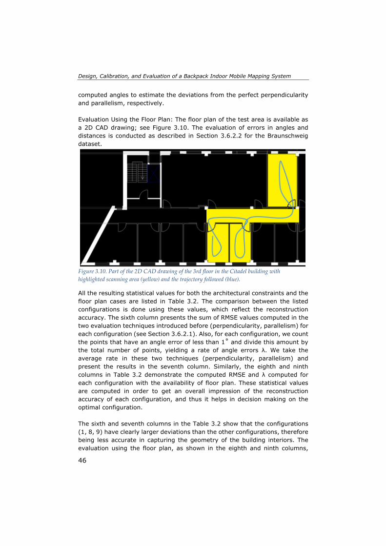
Design, Calibration, and Evaluation of a Backpack Indoor Mobile Mapping System

46

computed angles to estimate the deviations from the perfect perpendicularity and parallelism, respectively. Evaluation Using the Floor Plan: The floor plan of the test area is available as a 2D CAD drawing; see Figure 3.10. The evaluation of errors in angles and distances is conducted as described in Section 3.6.2.2 for the Braunschweig dataset.

Figure 3.10. Part of the 2D CAD drawing of the 3rd floor in the Citadel building with highlighted scanning area (yellow) and the trajectory followed (blue).

All the resulting statistical values for both the architectural constraints and the floor plan cases are listed in Table 3.2. The comparison between the listed configurations is done using these values, which reflect the reconstruction accuracy. The sixth column presents the sum of RMSE values computed in the two evaluation techniques introduced before (perpendicularity, parallelism) for each configuration (see Section 3.6.2.1). Also, for each configuration, we count the points that have an angle error of less than 1˚ and divide this amount by the total number of points, yielding a rate of angle errors λ. We take the average rate in these two techniques (perpendicularity, parallelism) and present the results in the seventh column. Similarly, the eighth and ninth columns in Table 3.2 demonstrate the computed RMSE and λ computed for each configuration with the availability of floor plan. These statistical values are computed in order to get an overall impression of the reconstruction accuracy of each configuration, and thus it helps in decision making on the optimal configuration. The sixth and seventh columns in the Table 3.2 show that the configurations (1, 8, 9) have clearly larger deviations than the other configurations, therefore being less accurate in capturing the geometry of the building interiors. The evaluation using the floor plan, as shown in the eighth and ninth columns,

Chapter 3

47

confirms this conclusion. RMSE values for parallelism indicate that the configurations (2-7, 10, 11) are the most accurate in maintaining an accurate localization when moving from one room to another. The common characteristic of these configurations is that they have at least one of the two rotation angles in the range of 30˚ to 40˚.

3.7.2.2 Completeness of Data Capturing We visually inspect the completeness of the captured data in which walls, floor, and ceiling are recorded. The process relies on a simulated point cloud representing a scan of a virtual corridor (loop) and generated for each configuration. Figure 3.11a shows the 3D model of this virtual area and Figure 3.11b the point cloud of configuration 6 where the colors relate to the three different LRFs and the white polyline represents the followed trajectory. The simulated point cloud generating process assumes that the operator walks around the corridor in an anti-clockwise direction starting from the middle of the corridor. The analysis process is based on a set of point clouds corresponding to all suggested configurations to compare the areas covered by points and find which configuration provides the better coverage. We want to investigate whether a more accurate configuration in geometry reconstruction could also provide a more complete point cloud of the scene. Overall, configurations (1-8) appear to give good coverage. However, the configurations (2, 3, 5, 7) provide the most complete point cloud of the scene, while the LRFs with the other configurations miss the lower/upper part of the wall in the scanning geometry when the system turns around the corner. An example of a configuration (6), which results in an incomplete point cloud, is shown in Figure 3.11b. This configuration misses a part of the wall close to the corner (see Figure 3.11c). Figure 3.11d shows the data recorded in one scan line of each LRF in the configuration 6. The tenth column in Table 3.2 demonstrate that the configurations (9, 10, 11) present the largest gaps in their point clouds. The common characteristic of these configurations is that only one of the slanted LRFs is scanning the walls both right and left of the system.

Design, Calibration, and Evaluation of a Backpack Indoor Mobile Mapping System

48

Figure 3.11. Simulation data. (a) 3D model of the virtual corridor used as a test area with the trajectory followed (white). (b) The resulting point cloud of the test area for the configuration 6 without ceiling’s points. The yellow dashed rectangle shows an example of a gap on the wall around the corner (c). (d) The simulated geometry of LRFs’ scanlines for the configuration 6 in which the colours relate to the three different LRFs (𝑆𝑆0 𝑔𝑔𝑟𝑟𝑒𝑒𝑒𝑒𝑛𝑛, 𝑆𝑆1 𝑝𝑝𝑝𝑝𝑟𝑟𝑝𝑝𝑙𝑙𝑒𝑒, 𝑆𝑆2 red).

3.7.3 Discussion of Configuration Experiments The results of sections 3.7.1. and 3.7.2. lead to the conclusion that the more accurate configuration in geometry reconstruction does not necessarily provide a more complete point cloud of the scene, and vice versa. Although the configurations (10, 11) show a better performance than configurations (2, 8) in terms of the reconstruction accuracy, they provide a less complete point cloud. Finally, our system has the top LRF mounted horizontally and on a level that the environment is not occluded by the operator’s head. The shadow area of this LRF is pointed to the wall either to the left or right of the operator. We discovered that the other two LRFs should be scanning the surfaces parallel to the moving direction e.g., walls both right and left of the system. Also, we found out that these LRFs should be rotated not only about the shoulder axis ( 𝑑𝑑𝑓𝑓), but at least one of them should also be rotated around the moving direction ( 𝑑𝑑𝑓𝑓) by an angle in the range of 30˚ to 40˚. Moreover, the results revealed that determining where the LRFs’ data gap is pointing at plays a

Chapter 3

49

pivotal role in the completeness of the resulting point clouds. The best coverage among the tested configurations was achieved when the gap of one slanted LRF was aimed at the floor and the gap of other was aimed at the ceiling. 3.8 Conclusions and Future Work We presented the design, calibration and registration methods, and performance analysis of a multi-sensor backpack indoor mobile mapping system (ITC- Backpack). We have proposed and presented several evaluation techniques for the investigation of the system’s ability to acquire geometric information of an interior environment. Evaluations can also be performed when there is no ground truth model or only a floor plan available. If the floor plan is outdated, this will usually surface as a large error in the evaluation and can therefore be identified as outlier. The results on the Braunschweig data showed some differences in the width of some walls between the floor plan and the realised construction. Such changed walls can then be removed from the analysis. The proposed evaluation methods are not limited to our mapping system. The experimental results showed the ability of ITC-Backpack to map an office building with an angle error within 1.5˚between its planar wall surfaces and the precision in generating the width of wall was around 1 cm. Although we did not consider the errors in the outdated floor plan, the point cloud-based map shows a good internal consistency. We have carried out an experimental comparison of selected configurations to find the best configuration by studying the properties of 3D planes and point clouds reconstructed with these configurations. The selection of the optimal sensor configuration was built in terms of data occlusion, the success of the algorithm, and the accuracy and completeness of the resulting map and point cloud. In order to see all walls around the system, we left the top LRF mounted horizontally in the optimal configuration for the backpack system and on a level that the environment cannot be occluded by the operator’s head. To achieve a good coverage of the surfaces both behind and in front of the system, it must be rotated around its axis to locate the shadow area on the wall either to the left or right of the operator. The other two LRFs should be scanning the surfaces parallel to the moving direction. Also, they should be rotated not only about the shoulder axis, but at least one of them should also be rotated about the moving direction by an angle in the range of 30˚ to 40˚. The gap in the sensor's field of view of one should be pointed at the floor, while the gap of other should be pointed at the ceiling. In this way, the system achieves improved coverage of the environment and ensures a good data association when passing through

Design, Calibration, and Evaluation of a Backpack Indoor Mobile Mapping System

50

doors and corners, and thus has a robust estimation of the plane and pose parameters. Nevertheless, the analysis of the system’s performance may be slightly different in another indoor environment with much larger or smaller spaces. For such environments we would then need to repeat the configuration optimization experiments presented in Section 3.7, but we do not expect this will be necessary for many buildings. In the near future, we plan to expand the scope of application of the current system and SLAM algorithm to include more complex situations such as staircases and fancy architecture (e.g., slanted walls, round walls, non-horizontal floor). To do that, we will integrate IMU data in the local pose estimation and as a consequence we can use higher order splines to predict future poses. We anticipate that this integration will lead to a better hypothesis generation of planar structures and an optimal estimation for the whole trajectory.

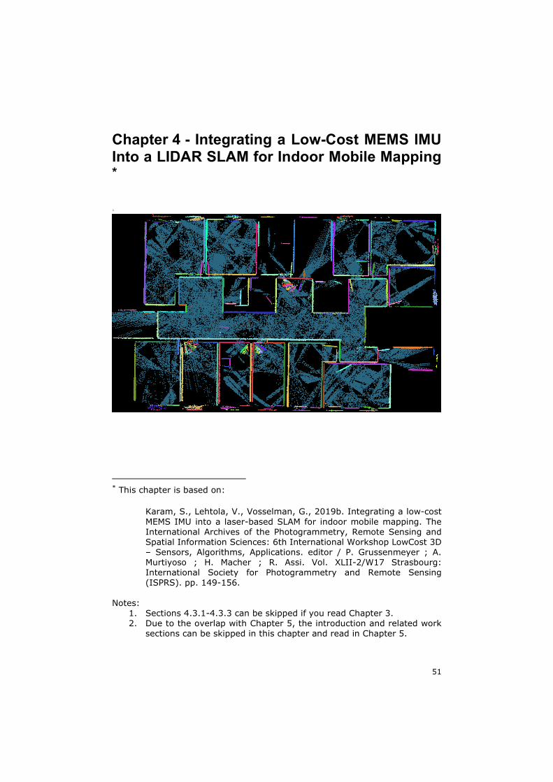
51

Chapter 4 - Integrating a Low-Cost MEMS IMU Into a LIDAR SLAM for Indoor Mobile Mapping *

1

* This chapter is based on:

Karam, S., Lehtola, V., Vosselman, G., 2019b. Integrating a low-cost MEMS IMU into a laser-based SLAM for indoor mobile mapping. The International Archives of the Photogrammetry, Remote Sensing and Spatial Information Sciences: 6th International Workshop LowCost 3D – Sensors, Algorithms, Applications. editor / P. Grussenmeyer ; A. Murtiyoso ; H. Macher ; R. Assi. Vol. XLII-2/W17 Strasbourg: International Society for Photogrammetry and Remote Sensing (ISPRS). pp. 149-156.

Notes: 1. Sections 4.3.1-4.3.3 can be skipped if you read Chapter 3. 2. Due to the overlap with Chapter 5, the introduction and related work

sections can be skipped in this chapter and read in Chapter 5.

Integrating a Low-Cost MEMS IMU Into a LIDAR SLAM for Indoor Mobile Mapping

52

Abstract Indoor mapping techniques are highly important in many applications, such as human navigation and indoor modelling. As satellite positioning systems do not work in indoor applications, several alternative navigational sensors and methods have been used to provide accurate indoor positioning for mapping purposes, such as inertial measurement units (IMUs) and simultaneous localisation and mapping algorithms (SLAM). In this chapter, we investigate the benefits that the integration of a low-cost microelectromechanical system (MEMS) IMU can bring to a feature-based SLAM algorithm. Specifically, we utilize IMU data to predict the pose of our backpack indoor mobile mapping system to improve the SLAM algorithm. The experimental results show that using the proposed IMU integration method leads into a more robust data association between the measured points and the model planes. Notably, the number of points that are assigned to the model planes is increased, and the root mean square error (RMSE) of the residuals, i.e., distances between these measured points and the model planes, is decreased significantly from 1.8 cm to 1.3 cm.

Chapter 4

53

4.1 Introduction There is a need for indoor mapping in many important applications, such as the mapping of hazardous sites, indoor navigation, disaster management, location-based services, and virtual reality displays. Since digital maps of public buildings (airports, hospitals, train stations, and so forth) are a prerequisite for navigating their interiors, there is a trend towards the development of geospatial indoor applications (Norris, 2013). In order to avoid the time-consuming and intense efforts that static mapping systems require to map building interiors, there has been increasing interest in indoor mobile mapping systems in recent years (Lehtola et al., 2017). As GNSS-based systems do not work indoors, several alternative navigational methods and sensors have been used to provide accurate indoor positioning for mapping purposes, such as simultaneous localisation and mapping algorithms (SLAMs) and inertial measurement units (IMUs). The essential solution methods and computational complexity of the SLAM problem are described by Durrant-Whyte and Bailey (2006a, 2006b). SLAM has become a key technology in indoor mapping applications, and a wide variety of different SLAM algorithms have been proposed. These algorithms are based on data from cameras (Henry et al., 2014), laser scanners like HectorSLAM (Kohlbrecher et al., 2011) and Gmapping (Grisetti et al., 2007), (Lehtola et al., 2016; Wen et al., 2016)) or both (Liu et al., 2010; Naikal et al., 2009). Surveys, as conducted by Maximov (2013), have shown that the integration of multiple sources of navigational information improves the accuracy of a navigation system. IMUs are one of the most commonly used navigational data sources in attitude (Hyyti et al., 2015; Makni et al., 2014) and pose estimation methods (Feliz et al., 2009). In addition to being relatively inexpensive, the MEMS-based IMUs are relatively small in size, lightweight, and low in power consumption; as such, they are widely integrated into indoor navigation systems. For example, an IMU is fused with a Hokuyo scanner on unmanned aerial vehicles (UAVs) (Kumar et al., 2017) and with a Velodyne scanner and panorama camera on backpack platforms (Blaser et al., 2019). Many works have integrated visual and inertial sensors within indoor SLAM algorithms (Chow et al., 2014; Concha et al., 2016; García et al., 2016; Leutenegger et al., 2015; Wang et al., 2018). However, the camera-based SLAM algorithms fail in textureless or repetitive environments because those algorithms search for similar features in consecutive images. Moreover, the light conditions in indoor environments are sometimes not good enough for capturing high-quality images. In our previous work (Karam et al., 2019), we built our feature-based SLAM algorithm based on three Hokuyo laser scanners. In this chapter, we

Integrating a Low-Cost MEMS IMU Into a LIDAR SLAM for Indoor Mobile Mapping

54

investigate the benefits obtained from integrating a low-cost microelectromechanical system (MEMS) IMU into this SLAM. Our effort is characterized by that we try to keep our system as inexpensive as possible by using less expensive LIDAR sensors with the low-cost IMU. All the involved sensors are mounted on a backpack platform, which provides more freedom than UAVs in terms of the weight of the mounted components. An IMU has strengths and weaknesses. Using only the IMU to navigate, the so-called dead reckoning leads to the drift of the predicted position from the physical one due to biases in the sensor observations (Jimenez et al., 2010). The IMU can provide reliable estimations of positions and attitudes for a short while, but its reliability decreases over time. In this work, we seek to exploit the strength of the IMU in measuring short-term pose changes and improving the pose prediction, thereby improving the data association robustness of the SLAM method. The remainder of this chapter is organized as follows: Section 4.2 presents the related works. Section 4.3 describes our backpack mapping system and the LIDAR SLAM algorithm. Then we elaborate the strategy used in the IMU-SLAM integration. In Section 4.4, we provide a brief overview of the datasets used to investigate this mapping technique. The analysis of the IMU performance is presented in Section 4.5. Section 4.6 discusses the results obtained from integrating the IMU with the LIDAR SLAM. Finally, Section 4.7 presents conclusions. 4.2 Related Work IMUs are widely used in indoor navigation and mapping systems. In addition to the works mentioned in the introduction, there are some specific ones that are closely related. For instance, an IMU is combined with one Hokuyo scanner and utilized for position estimation in 3D hand-held laser scanning system—ZEB-REVO1—evolved by GeoSLAM company. Blaser et al. (2019) incorporated MEMS IMU with two Velodyne VLP-16 laser scanners and one panorama camera in a portable mobile mapping system. The fusion of IMU and scanners in their SLAM is exploited to orient the camera in indoor environments. The Leica Pegasus backpack2 system also integrates a dual Velodyne VLP-16 scanner with a high precision IMU for indoor mapping. In addition, Lauterbach et al. (2015) presented a backpack mapping system equipped with 2D (SICK LMS 100) and 3D (Riegl VZ-400) laser scanners, and an IMU (Phidgets 1044). Two SLAM algorithms (3DOF HectorSLAM and 6DOF semi-rigid SLAM) execute successively, with the output of one being the input of the other. The first one,

1 www.geoslam.com 2 www.leica-geosystems.com

Chapter 4

55

HectorSLAM, uses the data of SICK scanner and an IMU for initial trajectory estimation. The semi-rigid SLAM exploits this initial pose estimation to align point clouds captured by the 3D scanner. The integration of IMU data can also be utilised to increase the degrees of freedom (DOF) of a mobile system. For instance, Wen et al. (2016) extended a horizontal laser-based 2D SLAM using rotations captured by an IMU to obtain a 3D (6DOF) pose and improve the accuracy of the 3D map. Recently, Velas et al. (2019) proposed another mobile backpack solution that combines a pair of Velodyne scanners with IMU and satellite positioning. This makes the system capable to work outdoors as well. The IMU is utilized in indoor applications to align the horizontal planes, such as floor and ceiling, with the XY plane in the 3D model. 4.3 LIDAR SLAM And IMU Integration In the following section, we first describe our mobile mapping system and the employed LIDAR SLAM algorithm. Then we introduce the methodology used to integrate IMU with SLAM. 4.3.1 System Components Our backpack indoor mobile mapping system consists of three time-of-flight (TOF) scanners (Hokuyo UTM-30LX) and one Xsens MEMS IMU. The top scanner is horizontally positioned and mounted on the top of the backpack system, while the other two scanners are tilted and mounted to the right and left of the top one, as shown in Figure 4.1. The IMU is horizontally positioned and mounted underneath the top scanner. A laptop running Ubuntu 16.04.X and the robot operation system (ROS) is used to communicate with all the mounted sensors and visualize the captured data over time. 4.3.2 Coordinate Systems and Registration Process Figure 4.1 shows the various coordinate systems in our backpack mapping system. In order to accurately fuse data from multiple sensors, their individual coordinate systems must be transformed into a unified coordinate system called the frame coordinate system (f). We adopt the coordinate system of the top scanner as the frame coordinate system. As described in our previous work (Karam et al., 2019), the two tilted scanners are registered in this frame coordinate system. For the relative rotation of the IMU with respect to the frame coordinate system, the z-axes of both the IMU and frame are assumed to be aligned by design. For full alignment, the IMU sensor system (s) need to be rotated around the z-axis through a 90˚ angle in a clockwise direction (𝑅𝑅𝑠𝑠

𝑓𝑓). As the frame system is constantly moving, we need to define a fixed coordinate system in which the final 3D model will be defined. Our fixed model system (m) is established from the first scans of the three scanners, as described by

Integrating a Low-Cost MEMS IMU Into a LIDAR SLAM for Indoor Mobile Mapping

56

Vosselman (2014). The moving frame system is registered in this model coordinate system over time 𝑡𝑡 using six transformation parameters, namely, three rotation parameters (𝜔𝜔𝑓𝑓t

𝑚𝑚, 𝜑𝜑𝑓𝑓t𝑚𝑚, 𝜅𝜅𝑓𝑓t

𝑚𝑚) form the rotation matrix 𝑅𝑅𝑓𝑓𝑡𝑡𝑚𝑚 and three

translation parameters (𝑑𝑑𝑓𝑓t𝑚𝑚, 𝑑𝑑𝑓𝑓𝑡𝑡

𝑚𝑚, 𝑑𝑑𝑓𝑓t𝑚𝑚) form the translation vector 𝑇𝑇𝑓𝑓𝑡𝑡

𝑚𝑚. These transformation parameters are estimated within the LIDAR SLAM.

Figure 4.1. The backpack system with coordinate systems plotted for all four mounted sensors: the three scanners S0, S1, and S2, and the Xsens IMU (below S0).

4.3.3 LIDAR SLAM LIDAR SLAM is a feature-based SLAM with 6DOF, three position (𝑇𝑇𝑓𝑓𝑡𝑡

𝑚𝑚) and three attitude (𝑅𝑅𝑓𝑓𝑡𝑡

𝑚𝑚) parameters. As the scanning frequency of the Hokuyo model used is 40 HZ, each scanner records one scanline within a local time window of 25 ms. Our SLAM senses planar features, horizontal and vertical, in the mapped environment through the linear segments that are detected in the single scanlines. We model the frame pose parameters as a function of time using B-splines and define each plane by its normal vector and distance to the origin in the model coordinate system. The solution of SLAM goes through two consecutive laser-based estimation processes, a local pose spline estimation involving the data captured during only 75-100 ms, and a global adjustment. The methods are explained in detail in Karam et al. (2019). In this chapter, we focus on the local spline estimation process in which the pose is predicted and the data association is tested. This estimation is based on the laser observations of only three to four scanlines from each of the scanners. The algorithm tries to establish the association

Chapter 4

57

between the linear segments in the three newly captured scanlines within the local window and the previously reconstructed planes. This test is based on the predicted pose resulting from a linear extrapolation of the locally estimated splines. It uses a distance threshold to decide whether a segment should be associated with a previously reconstructed plane or whether a new horizontal/vertical plane needs to be instantiated. When the whole dataset is processed locally, the SLAM runs a final adjustment process that estimates not only the trajectory parameters but also the parameters of all the reconstructed planes in the model coordinate system. 4.3.4 IMU-based Pose Prediction Here, we consider an Xsens MEMS IMU that is a combination of three-axial accelerometers used to measure dynamic acceleration and gravity and three-axial gyroscopes used to measure angular velocity. The accelerations and angular velocities are collected with a sampling frequency of 200 HZ; thus, there are few IMU measurements taken within each local window of one scanline. As an alternative to linear extrapolation, those measurements are utilized to provide a more reliable prediction of the system’s position and attitude, as described in the following subsections. We assume that the local window, for which we want to predict the pose, starts at 𝑡𝑡start and ends at 𝑡𝑡end. The IMU measurements are the angular velocities (�̇�𝜔𝑖𝑖𝑚𝑚𝑖𝑖

𝑠𝑠𝑡𝑡𝑖𝑖 , �̇�𝜑𝑖𝑖𝑚𝑚𝑖𝑖𝑠𝑠𝑡𝑡𝑖𝑖 , �̇�𝜅𝑖𝑖𝑚𝑚𝑖𝑖

𝑠𝑠𝑡𝑡𝑖𝑖 ) and accelerations (�̈�𝑑𝑖𝑖𝑚𝑚𝑖𝑖𝑠𝑠𝑡𝑡𝑖𝑖 , �̈�𝑑𝑖𝑖𝑚𝑚𝑖𝑖

𝑠𝑠𝑡𝑡𝑖𝑖 , �̈�𝑑𝑖𝑖𝑚𝑚𝑖𝑖𝑠𝑠𝑡𝑡𝑖𝑖 ) observed at time 𝑡𝑡𝑖𝑖 in the

IMU sensor system(s), where 𝑖𝑖 =1, 2, … ,n. We select 𝑡𝑡1 as the timestamp of the last IMU measurement before 𝑡𝑡start and 𝑡𝑡𝑛𝑛 as the timestamp of the first IMU measurement after 𝑡𝑡end. The following pose parameters are known at 𝑡𝑡1 from the SLAM estimation process that ran before: - The attitude parameters (𝜔𝜔𝑓𝑓𝑡𝑡1,slam

𝑚𝑚 , 𝜑𝜑𝑓𝑓𝑡𝑡1,slam

𝑚𝑚 , 𝜅𝜅𝑓𝑓𝑡𝑡1,slam

𝑚𝑚 ) form the rotation matrix

𝑅𝑅𝑓𝑓𝑡𝑡1,slam

𝑚𝑚 from the frame coordinate system to the world coordinate system at 𝑡𝑡1.

𝑅𝑅𝑓𝑓𝑡𝑡1,slam𝑚𝑚 = 𝑅𝑅1(𝜔𝜔𝑓𝑓𝑡𝑡1,slam

𝑚𝑚 )𝑅𝑅2(𝜑𝜑𝑓𝑓𝑡𝑡1,slam𝑚𝑚 ) 𝑅𝑅3(𝜅𝜅𝑓𝑓𝑡𝑡1,slam

𝑚𝑚 ) (4.1)

- The position parameters �𝑑𝑑𝑓𝑓𝑡𝑡1,slam

𝑚𝑚 , 𝑑𝑑𝑓𝑓𝑡𝑡1,slam

𝑚𝑚 , 𝑑𝑑𝑓𝑓𝑡𝑡1,slam

𝑚𝑚 � form the translation vector 𝑇𝑇𝑓𝑓𝑡𝑡1,slam

𝑚𝑚 from the frame coordinate system to the world coordinate system at 𝑡𝑡1.

𝑇𝑇𝑓𝑓𝑡𝑡1,slam

𝑚𝑚 = �𝑑𝑑𝑓𝑓𝑡𝑡1,slam𝑚𝑚 , 𝑑𝑑𝑓𝑓𝑡𝑡1,slam

𝑚𝑚 , 𝑑𝑑𝑓𝑓𝑡𝑡1,slam𝑚𝑚 �

𝑇𝑇 (4.2)

Integrating a Low-Cost MEMS IMU Into a LIDAR SLAM for Indoor Mobile Mapping

58

- The approximate velocity of the frame in the model coordinate system at time 𝑡𝑡1.

�̇�𝑇𝑓𝑓𝑡𝑡1,slam𝑚𝑚 = ��̇�𝑑𝑓𝑓𝑡𝑡1,slam

𝑚𝑚 , �̇�𝑑𝑓𝑓𝑡𝑡1,slam𝑚𝑚 , �̇�𝑑𝑓𝑓𝑡𝑡1,slam

𝑚𝑚 �𝑇𝑇 (4.3)

4.3.4.1 Attitude The three attitude parameters can be determined by integrating time with the angular velocity. Since the IMU observes angular velocities in the IMU sensor system (s), they need to be rotated to the frame coordinate system (f) with the time-independent rotation matrix 𝑅𝑅𝑠𝑠

𝑓𝑓.

⎝

⎜⎛�̇�𝜔𝑖𝑖𝑚𝑚𝑖𝑖𝑓𝑓𝑡𝑡𝑖𝑖

�̇�𝜑𝑖𝑖𝑚𝑚𝑖𝑖𝑓𝑓𝑡𝑡𝑖𝑖

�̇�𝜅𝑖𝑖𝑚𝑚𝑖𝑖𝑓𝑓𝑡𝑡𝑖𝑖

⎠

⎟⎞

= 𝑅𝑅𝑠𝑠𝑓𝑓

⎝

⎜⎛�̇�𝜔𝑖𝑖𝑚𝑚𝑖𝑖𝑠𝑠𝑡𝑡𝑖𝑖

�̇�𝜑𝑖𝑖𝑚𝑚𝑖𝑖𝑠𝑠𝑡𝑡𝑖𝑖

�̇�𝜅𝑖𝑖𝑚𝑚𝑖𝑖𝑠𝑠𝑡𝑡𝑖𝑖

⎠

⎟⎞

(4.4)

We obtain the incremental angles of the frame rotation from 𝑡𝑡𝑖𝑖 to 𝑡𝑡𝑖𝑖+1. If we multiply the angular velocities in the frame coordinate system by Δ𝑡𝑡 = 𝑡𝑡𝑖𝑖+1 − 𝑡𝑡𝑖𝑖, we arrive at:

𝑅𝑅𝑓𝑓𝑡𝑡𝑖𝑖𝑓𝑓𝑡𝑡𝑖𝑖+1 = 𝑅𝑅1 ��̇�𝜔𝑖𝑖𝑚𝑚𝑖𝑖

𝑓𝑓𝑡𝑡𝑖𝑖 Δ𝑡𝑡� 𝑅𝑅2 ��̇�𝜑𝑖𝑖𝑚𝑚𝑖𝑖𝑓𝑓𝑡𝑡𝑖𝑖 Δ𝑡𝑡� 𝑅𝑅3 ��̇�𝜅𝑖𝑖𝑚𝑚𝑖𝑖

𝑓𝑓𝑡𝑡𝑖𝑖 Δ𝑡𝑡� (4.5)

Then, the rotation matrix 𝑅𝑅𝑓𝑓𝑡𝑡𝑖𝑖+1

𝑚𝑚 from the frame coordinate system to the model

coordinate system at 𝑡𝑡𝑖𝑖+1 can be computed as follows:

𝑅𝑅𝑓𝑓𝑡𝑡𝑖𝑖+1𝑚𝑚 = 𝑅𝑅𝑓𝑓𝑡𝑡𝑖𝑖

𝑚𝑚 (𝑅𝑅𝑓𝑓𝑡𝑡𝑖𝑖𝑓𝑓𝑡𝑡𝑖𝑖+1)𝑇𝑇 (4.6)

where 𝑅𝑅𝑓𝑓𝑡𝑡𝑖𝑖

𝑚𝑚= 𝑅𝑅𝑓𝑓𝑡𝑡1,slam

𝑚𝑚 , if 𝑖𝑖 = 1, and 𝑅𝑅𝑓𝑓𝑡𝑡𝑖𝑖𝑚𝑚= 𝑅𝑅𝑓𝑓𝑡𝑡𝑖𝑖−1

𝑚𝑚 otherwise.

From the resulting rotation matrix 𝑅𝑅𝑓𝑓𝑡𝑡𝑖𝑖+1

𝑚𝑚 , we can infer the predicted attitude

parameters (rotation angles) at 𝑡𝑡𝑖𝑖+1, 𝜔𝜔𝑓𝑓𝑡𝑡i+1𝑚𝑚 , 𝜑𝜑𝑓𝑓𝑡𝑡𝑖𝑖+1

𝑚𝑚 , 𝜅𝜅𝑓𝑓𝑡𝑡𝑖𝑖+1𝑚𝑚 .

4.3.4.2 Position The three position parameters can be derived via the double integration of the acceleration. The IMU also observes accelerations in its sensor system and can

Chapter 4

59

be rotated to the model coordinate system using the 𝑅𝑅𝑠𝑠𝑓𝑓 and 𝑅𝑅𝑓𝑓𝑡𝑡𝑖𝑖

𝑚𝑚 predicted above

as follows:

��̈�𝑑𝑖𝑖𝑚𝑚𝑖𝑖_𝑡𝑡𝑖𝑖𝑚𝑚

�̈�𝑑𝑖𝑖𝑚𝑚𝑖𝑖_𝑡𝑡𝑖𝑖𝑚𝑚

�̈�𝑑𝑖𝑖𝑚𝑚𝑖𝑖_𝑡𝑡𝑖𝑖𝑚𝑚

� = 𝑅𝑅𝑓𝑓𝑡𝑡𝑖𝑖𝑚𝑚 𝑅𝑅𝑠𝑠

𝑓𝑓

⎝

⎜⎛�̈�𝑑𝑖𝑖𝑚𝑚𝑖𝑖𝑠𝑠𝑡𝑡𝑖𝑖

�̈�𝑑𝑖𝑖𝑚𝑚𝑖𝑖𝑠𝑠𝑡𝑡𝑖𝑖

�̈�𝑑𝑖𝑖𝑚𝑚𝑖𝑖𝑠𝑠𝑡𝑡𝑖𝑖

⎠

⎟⎞

(4.7)

As the accelerations are now resolved in the model system where the z-axis is assumed to be vertical, we subtract the average gravity (𝑔𝑔) from the acceleration along this axis.

�̈�𝑇𝑖𝑖𝑚𝑚𝑖𝑖_𝑡𝑡𝑖𝑖𝑚𝑚 = �

�̈�𝑑𝑖𝑖𝑚𝑚𝑖𝑖_𝑡𝑡𝑖𝑖𝑚𝑚

�̈�𝑑𝑖𝑖𝑚𝑚𝑖𝑖_𝑡𝑡𝑖𝑖𝑚𝑚

�̈�𝑑𝑖𝑖𝑚𝑚𝑖𝑖_𝑡𝑡𝑖𝑖𝑚𝑚 − 𝑔𝑔

� (4.8)

Using these accelerations and the known frame position and velocity at 𝑡𝑡𝑖𝑖, we can obtain the frame position and velocity at 𝑡𝑡𝑖𝑖+1 as follows:

𝑇𝑇𝑓𝑓𝑡𝑡𝑖𝑖+1𝑚𝑚 = 𝑇𝑇𝑓𝑓𝑡𝑡𝑖𝑖

𝑚𝑚 + Δ𝑡𝑡 �̇�𝑇𝑓𝑓𝑡𝑡𝑖𝑖𝑚𝑚 +

12Δ𝑡𝑡2 �̈�𝑇𝑖𝑖𝑚𝑚𝑖𝑖_𝑡𝑡𝑖𝑖

𝑚𝑚 (4.9)

�̇�𝑇𝑓𝑓𝑡𝑡𝑖𝑖+1

𝑚𝑚 = �̇�𝑇𝑓𝑓𝑡𝑡𝑖𝑖𝑚𝑚 + Δ𝑡𝑡 �̈�𝑇𝑖𝑖𝑚𝑚𝑖𝑖_𝑡𝑡𝑖𝑖

𝑚𝑚 (4.10)

where �̇�𝑇𝑓𝑓𝑡𝑡𝑖𝑖

𝑚𝑚= �̇�𝑇𝑓𝑓𝑡𝑡1,slam

𝑚𝑚 and 𝑇𝑇𝑓𝑓𝑡𝑡𝑖𝑖𝑚𝑚 = 𝑇𝑇𝑓𝑓𝑡𝑡1,slam

𝑚𝑚 , if 𝑖𝑖 = 1, and �̇�𝑇𝑓𝑓𝑡𝑡𝑖𝑖𝑚𝑚= �̇�𝑇𝑓𝑓𝑡𝑡𝑖𝑖−1

𝑚𝑚 and 𝑇𝑇𝑓𝑓𝑡𝑡𝑖𝑖𝑚𝑚 =

𝑇𝑇𝑓𝑓𝑡𝑡𝑖𝑖−1𝑚𝑚 otherwise.

4.3.5 SLAM and IMU Integration The IMU fusion with the SLAM system is based mainly on the replacement of linear extrapolation by the IMU-based prediction, Eq. (4.6) and Eq. (4.10), to test the data association within the local window. Here, we fit cubic splines through all the predicted poses (six cubic splines for six pose parameters) and used these splines to test the data association. 4.4 Datasets Two datasets were captured with the backpack mapping system and used in this work. The first dataset is collected in a cube-shaped room with some bending movements. Specifically, the operator first stands inside a room with

Integrating a Low-Cost MEMS IMU Into a LIDAR SLAM for Indoor Mobile Mapping

60

planar and vertical structures, which represents an optimal environment for our SLAM. Then the operator starts recording data with the scanners and IMU while bending forward and sideward (right and left), then rotating 90˚ to perform these bends again. The operator continues the rotation and bending steps until he or she is back at the starting orientation. The dataset collected in this manner is then utilized for IMU data analysis, as described in Section 4.5.1. The second dataset was acquired at the University of Braunschweig, Germany. The scanned floor shows a distinct office environment. It is the main dataset used in this study and was utilized to investigate the IMU prediction in comparison with linear extrapolation and show the benefits of the IMU-SLAM integration, as described in Sections 4.5.2 and 4.6. 4.5 Analysis of IMU Performance 4.5.1 IMU Data Analysis In order to analyse the IMU data, we check the consistency of the IMU angular velocity with the first-order derivatives of the rotation splines estimated by the LIDAR SLAM. We run the SLAM on the first dataset because we have large changes in rotation around all three axes, and we want to check if the approximate values of rotational rates estimated by SLAM show the same pattern as the rotational rates measured by the IMU. The angular velocities (�̇�𝜔𝑖𝑖𝑚𝑚𝑖𝑖

s , �̇�𝜑𝑖𝑖𝑚𝑚𝑖𝑖s , �̇�𝜅𝑖𝑖𝑚𝑚𝑖𝑖s ) measured by the IMU are observed around the axes of the IMU sensor. What we need are the partial derivatives of the rotation angles (splines) estimated by SLAM and used to rotate between the model and the frame coordinate system, i.e., �̇�𝜔𝑓𝑓,𝑠𝑠𝑠𝑠𝑠𝑠𝑚𝑚

𝑚𝑚 , �̇�𝜑f,slam𝑚𝑚 , �̇�𝜅𝑓𝑓,𝑠𝑠𝑠𝑠𝑠𝑠𝑚𝑚𝑚𝑚 . To determine the

relationship with the observed angular velocities, we first need to define the order and direction of rotation exactly. So far, we have defined 𝑅𝑅f𝑚𝑚 using Eq. (4.1); hence, the rotation from the model coordinate system to the frame coordinate system 𝑅𝑅𝑚𝑚f can be defined as:

𝑅𝑅𝑚𝑚f = (𝑅𝑅f𝑚𝑚)𝑇𝑇 = 𝑅𝑅3�𝜅𝜅𝑓𝑓,𝑠𝑠𝑠𝑠𝑠𝑠𝑚𝑚𝑚𝑚 �𝑇𝑇𝑅𝑅2�𝜑𝜑𝑓𝑓,𝑠𝑠𝑠𝑠𝑠𝑠𝑚𝑚

𝑚𝑚 �𝑇𝑇𝑅𝑅1�ω𝑓𝑓,𝑠𝑠𝑠𝑠𝑠𝑠𝑚𝑚𝑚𝑚 �𝑇𝑇 (4.11)

Once the model coordinate system is aligned with the frame coordinate system,

we can apply the time-independent rotation 𝑅𝑅𝑓𝑓𝑆𝑆 = �𝑅𝑅𝑠𝑠𝑓𝑓�

𝑇𝑇 from the frame to the

IMU sensor coordinate system. Here, the entire rotation from the model coordinate system to the IMU sensor coordinate system will be:

𝑅𝑅𝑚𝑚𝑠𝑠 = 𝑅𝑅𝑓𝑓𝑆𝑆𝑅𝑅𝑚𝑚𝑓𝑓 (4.12)

Chapter 4

61

As κ is the first rotation applied when rotating from the frame to the model coordinate system, we do not have to rotate the �̇�𝜅𝑠𝑠𝑠𝑠𝑠𝑠𝑚𝑚𝑚𝑚 from the model to the frame. The measured angular velocity �̇�𝜑𝑖𝑖𝑚𝑚𝑖𝑖s around the y-axis does not correspond directly to the first derivative of 𝜑𝜑𝑓𝑓,𝑠𝑠𝑠𝑠𝑠𝑠𝑚𝑚

𝑚𝑚 when just rotating (𝑅𝑅𝑓𝑓𝑆𝑆) from the frame to the IMU sensor coordinate system because the y-axis has already been rotated by −𝜅𝜅𝑓𝑓,𝑠𝑠𝑠𝑠𝑠𝑠𝑚𝑚

𝑚𝑚 around the z-axis prior to measuring �̇�𝜑𝑖𝑖𝑚𝑚𝑖𝑖s in the IMU sensor coordinate system. Hence, the derivative of 𝜑𝜑𝑓𝑓,𝑠𝑠𝑠𝑠𝑠𝑠𝑚𝑚

𝑚𝑚 should also be rotated to the frame coordinate system. Similarly, the derivative of 𝜔𝜔𝑓𝑓,𝑠𝑠𝑠𝑠𝑠𝑠𝑚𝑚

𝑚𝑚 needs to be rotated by −𝜑𝜑𝑓𝑓,𝑠𝑠𝑠𝑠𝑠𝑠𝑚𝑚

𝑚𝑚 around the y-axis and −𝜅𝜅𝑓𝑓,𝑠𝑠𝑠𝑠𝑠𝑠𝑚𝑚𝑚𝑚 around the z-axis to obtain

an angular velocity vector in the frame coordinate system. So, all the rotated angular velocity vectors together determine the angular rotation velocities that are measured in the frame coordinate system. Hence, after rotating from the frame to the IMU coordinate system, we obtain the angular velocities as derived by the SLAM in the IMU coordinate system as

��̇�𝜔𝑠𝑠𝑠𝑠𝑠𝑠𝑚𝑚𝑆𝑆

�̇�𝜑𝑠𝑠𝑠𝑠𝑠𝑠𝑚𝑚𝑆𝑆

�̇�𝜅𝑠𝑠𝑠𝑠𝑠𝑠𝑚𝑚𝑆𝑆� = 𝑅𝑅𝑓𝑓𝑆𝑆 �

00

�̇�𝜅𝑓𝑓,𝑠𝑠𝑠𝑠𝑠𝑠𝑚𝑚𝑚𝑚

� +

𝑅𝑅𝑓𝑓𝑆𝑆𝑅𝑅3�𝜅𝜅𝑓𝑓,𝑠𝑠𝑠𝑠𝑠𝑠𝑚𝑚𝑚𝑚 �𝑇𝑇 �

0�̇�𝜑f,slam𝑚𝑚

0�𝑅𝑅𝑓𝑓𝑆𝑆𝑅𝑅3�𝜅𝜅𝑓𝑓,𝑠𝑠𝑠𝑠𝑠𝑠𝑚𝑚

𝑚𝑚 �𝑇𝑇𝑅𝑅2�𝜑𝜑𝑓𝑓,𝑠𝑠𝑠𝑠𝑠𝑠𝑚𝑚𝑚𝑚 �𝑇𝑇 �

�̇�𝜔𝑓𝑓,𝑠𝑠𝑠𝑠𝑠𝑠𝑚𝑚m

00

�

These angular velocities should be comparable to those measured by the IMU. To verify this, the angular velocities (�̇�𝜔𝑠𝑠𝑠𝑠𝑠𝑠𝑚𝑚

s , �̇�𝜑𝑠𝑠𝑠𝑠𝑠𝑠𝑚𝑚s , �̇�𝜅𝑠𝑠𝑠𝑠𝑠𝑠𝑚𝑚s ) are plotted against (�̇�𝜔𝑖𝑖𝑚𝑚𝑖𝑖

s , �̇�𝜑𝑖𝑖𝑚𝑚𝑖𝑖s , �̇�𝜅𝑖𝑖𝑚𝑚𝑖𝑖s ) and the differences are computed. Figure 4.2 shows �̇�𝜑𝑓𝑓,𝑠𝑠𝑠𝑠𝑠𝑠𝑚𝑚𝑆𝑆

plotted against �̇�𝜑𝑖𝑖𝑚𝑚𝑖𝑖𝑆𝑆 . After the burn-off period of 0.2 s, the results are promising because both the IMU- and SLAM- based angular velocities exhibit the same patterns. The differences between the IMU and SLAM angular velocities along all axes are mostly within ±0.05ᵒ-0.1ᵒ/s.

(4.13)

Integrating a Low-Cost MEMS IMU Into a LIDAR SLAM for Indoor Mobile Mapping

62

Figure 4.2. An example plot for testing the IMU integration. The angular velocities measured by the IMU along the y-axis are plotted against the first-order derivatives of the rotation y-splines estimated by the LIDAR SLAM. Similar tests were done for all axes of the gyroscope.

4.5.2 IMU Prediction Analysis We run the LIDAR SLAM on the second dataset. As an initial analysis of the SLAM-IMU combined performance, we use the IMU data to predict the pose of the next scan (𝑃𝑃𝑝𝑝𝑟𝑟𝑝𝑝𝑝𝑝𝑖𝑖𝑚𝑚𝑖𝑖 ) using the equations introduced in Section 4.3.4 and compare the resulting pose with the linearly predicted one (𝑃𝑃𝑝𝑝𝑟𝑟𝑝𝑝𝑝𝑝𝑠𝑠𝑖𝑖𝑛𝑛𝑝𝑝𝑠𝑠𝑟𝑟). As ground truth we use the poses (𝑃𝑃𝑝𝑝𝑠𝑠𝑡𝑡) obtained in the optimal global pose estimation of the SLAM procedure. Figure 4.3 shows that the predicted rotation angles around the X-axis (ω) and Z-axis (κ) by the IMU are closer to the ground truth angles than the linearly predicted ones. Table 4.1 lists the RMSE values computed using Eq. (4.14) for all the pose parameters, namely, the rotation angles (ω, ϕ, κ) and positions (X, Y, Z).

𝑅𝑅𝑅𝑅𝑆𝑆𝐸𝐸𝑃𝑃𝑚𝑚𝑝𝑝𝑡𝑡ℎ = �1𝑁𝑁��𝑃𝑃𝑝𝑝𝑟𝑟𝑝𝑝𝑝𝑝_𝑖𝑖

𝑚𝑚𝑝𝑝𝑡𝑡ℎ − 𝑃𝑃𝑝𝑝𝑠𝑠𝑡𝑡_𝑖𝑖�2

𝑁𝑁

𝑖𝑖=1

(4.14)

where P refers to one of the pose parameters {x, y, z, ω, φ, κ} , 𝑃𝑃𝑝𝑝𝑠𝑠𝑡𝑡 is the estimated pose parameter by the LIDAR SLAM. The term “meth” refers to the prediction method, “imu” when we rely on IMU for pose prediction and “linear” otherwise.

0 5 10 15 20 25 30 35 40 45

Time[s]

-1.5

-1

-0.5

0

0.5

1

1.5

Ang

V-Y[

deg/

s]

IMU

SLAM

Chapter 4

63

Table 4.1. RMSE values of all the predicted pose parameters, rotation angles, and position coordinates.

SLAM Rotation Angles

RMSE (deg) Position RMSE (m)

ω φ κ X Y Z

With IMU 0.092 0.106 0.100 0.0054 0.0033 0.0031

Without IMU 0.166 0.160 0.231 0.0054 0.0032 0.0032 The RMSE results indicate that the IMU prediction of orientation is about two times more accurate than the linear prediction. As the operator walking speed is usually less than 1.4 m/s, the expected translation between two scanlines (within 25 ms) is about 3 cm. Thus, the fractions of millimetres improvement in position prediction is irrelevant for data association. The most crucial issue is the orientation prediction, because the operator can make a large change in orientation within 25 ms or an even shorter time span. Moreover, a small error in the orientation prediction can have serious effects on the data association quality. As a simple example, if there is a point at a distance of 10 m from the system, a linear prediction error of the angle κ of one sigma (0.231˚) would already result in a 4.0 cm lateral displacement of this point compared to a 1.7 cm lateral displacement with the IMU prediction.

4.6 Integration Results And Discussion In order to test the performance of the IMU-SLAM integration, the IMU prediction-based SLAM was run on the second dataset. The generated point cloud is shown in Figure 4.4. In order to evaluate the benefits of this integration, we compare the number of points assigned to the planes and the RMSE of the residuals in two cases: SLAM with and without IMU prediction (Table 4.2). In this chapter, SLAM without IMU refers to the linear prediction- based SLAM. The residuals are the distances of the points to the estimated planes.

Integrating a Low-Cost MEMS IMU Into a LIDAR SLAM for Indoor Mobile Mapping

64

(a)

(b)

Figure 4.3. Part of the rotation angles (ω, κ) trajectories. (a) for ω. (b) for κ. Each blue line connects the two estimated angles (ω, κ) at the start and end of one local window (≈ 25 ms). The dashed black and red lines are the IMU and linear predictions of angles (ω, κ), respectively.

Chapter 4

65

Table 4.2. The number of assigned points and the corresponding RMSEs of the residuals.

SLAM Without IMU With IMU

Number of assigned points 24 527 978 24 562 619

RMSE of the residuals (cm) 1.80 1.31

The table shows that using the IMU data to predict the pose of the next scans slightly increases the number of points assigned to the planes. More importantly, the RMSE value of the points’ residuals with IMU prediction is quite a lot lower than that obtained via linear prediction, meaning that there are more correct associations when the IMU is used for pose prediction. In addition, histograms of the computed distances (residuals) between the assigned points and their corresponding reconstructed planes are generated in order to provide an overall impression of the data association quality in both cases. Each histogram is built with 0.01 m bins, as shown in Figure 4.5, demonstrating that approximately 13% of the residuals exceed 3 cm when the IMU is not used. This percentage decreases to less than 4% when the IMU is utilized in pose prediction.

Figure 4.4. A top view of the generated point cloud by SLAM with IMU. The colours indicate point associations to a particular plane.

Integrating a Low-Cost MEMS IMU Into a LIDAR SLAM for Indoor Mobile Mapping

66

Figure 4.5. Histograms of the points’ residuals in two cases, SLAM with and without IMU.

Since the perpendicularity and parallelism characteristics are predominant in the second indoor environment we scanned, we utilize our evaluation method with architectural constraints (Karam et al., 2018) to evaluate the ability of our updated mapping system to capture the true geometry of its environment. The method is applied with same thresholds on the reconstructed planes by SLAM in two cases, with and without IMU. We compute the angles between the (perpendicular/parallel) reconstructed planes and derive the deviations of these angles from the corresponding expected value (90º / 0º). The computed deviations are called angles’ errors. The results of this evaluation process are summarized in Tables (4.3, 4.4). Table 4.3. Percentages of angles’ errors for parallelism and perpendicularity in two cases, SLAM with and without IMU.

SLAM Errors range [0º 0.5º[ [0.5º 1º] >1º

With IMU parallelism 66% 13% 21%

perpendicularity 70% 23% 7%

Without IMU parallelism 50% 12% 38%

perpendicularity 58% 26% 16%

0 0.01 0.02 0.03 0.04 0.05 0.06 0.07 0.08 0.09 0.1

Residual [m]

0

10

20

30

40

50

60

70

Perc

enta

ge [%

]

Without IMU

With IMU

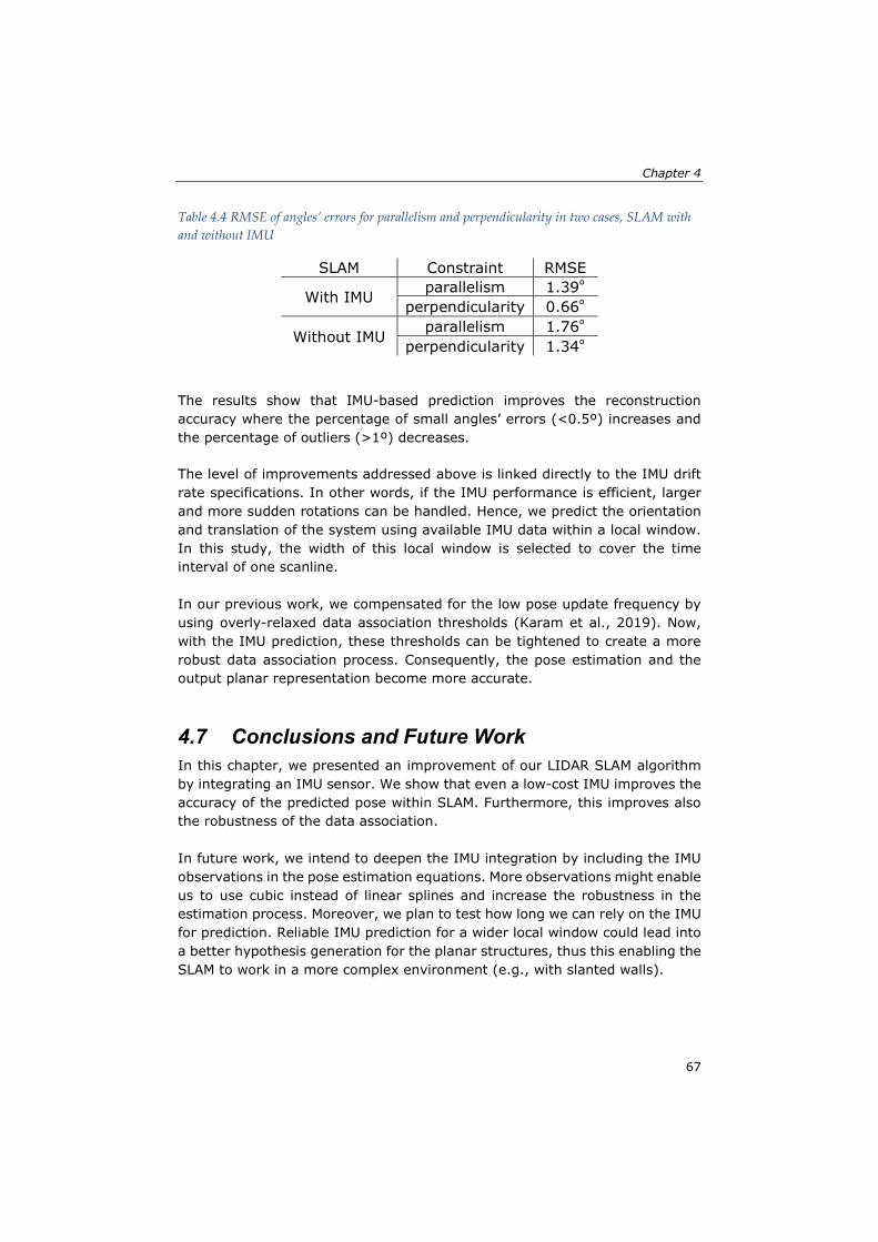
Chapter 4

67

Table 4.4 RMSE of angles’ errors for parallelism and perpendicularity in two cases, SLAM with and without IMU

SLAM Constraint RMSE

With IMU parallelism 1.39º

perpendicularity 0.66º

Without IMU parallelism 1.76º

perpendicularity 1.34º

The results show that IMU-based prediction improves the reconstruction accuracy where the percentage of small angles’ errors (<0.5º) increases and the percentage of outliers (>1º) decreases. The level of improvements addressed above is linked directly to the IMU drift rate specifications. In other words, if the IMU performance is efficient, larger and more sudden rotations can be handled. Hence, we predict the orientation and translation of the system using available IMU data within a local window. In this study, the width of this local window is selected to cover the time interval of one scanline. In our previous work, we compensated for the low pose update frequency by using overly-relaxed data association thresholds (Karam et al., 2019). Now, with the IMU prediction, these thresholds can be tightened to create a more robust data association process. Consequently, the pose estimation and the output planar representation become more accurate. 4.7 Conclusions and Future Work In this chapter, we presented an improvement of our LIDAR SLAM algorithm by integrating an IMU sensor. We show that even a low-cost IMU improves the accuracy of the predicted pose within SLAM. Furthermore, this improves also the robustness of the data association. In future work, we intend to deepen the IMU integration by including the IMU observations in the pose estimation equations. More observations might enable us to use cubic instead of linear splines and increase the robustness in the estimation process. Moreover, we plan to test how long we can rely on the IMU for prediction. Reliable IMU prediction for a wider local window could lead into a better hypothesis generation for the planar structures, thus this enabling the SLAM to work in a more complex environment (e.g., with slanted walls).

Integrating a Low-Cost MEMS IMU Into a LIDAR SLAM for Indoor Mobile Mapping

68

69

Chapter 5 - Strategies to Integrate IMU and LIDAR SLAM for Indoor Mapping *

1

* This chapter is based on:

Karam, S., Lehtola, V., and Vosselman, G.: Strategies to integrate imu and lidar slam for indoor mapping, ISPRS Ann. Photogramm. Remote Sens. Spatial Inf. Sci., V-1-2020, 223–230

Strategies to Integrate IMU and LIDAR SLAM for Indoor Mapping

70

Abstract In recent years, the importance of indoor mapping increased in a wide range of applications, such as facility management and mapping hazardous sites. The essential technique behind indoor mapping is simultaneous localization and mapping (SLAM) because SLAM offers suitable positioning estimates in environments where satellite positioning is not available. State-of-the-art indoor mobile mapping systems employ Visual SLAM or LIDAR SLAM. However, Visual SLAM is sensitive to textureless environments and, similarly, LIDAR SLAM is sensitive to a number of pose configurations where the geometry of laser observations is not strong enough to reliably estimate the six-degree-of-freedom (6DOF) pose of the system. In this chapter, we present different strategies that utilize the benefits of the inertial measurement unit (IMU) in the pose estimation and support LIDAR SLAM in overcoming these problems. The proposed strategies have been implemented and tested using different datasets and our experimental results demonstrate that the proposed methods do indeed overcome these problems. We conclude that IMU observations increase the robustness of SLAM, which is expected, but also that the best reconstruction accuracy is obtained not with a blind use of all observations but by filtering the measurements with a proposed reliability measure. To this end, our results show promising improvements in the reconstruction accuracy.

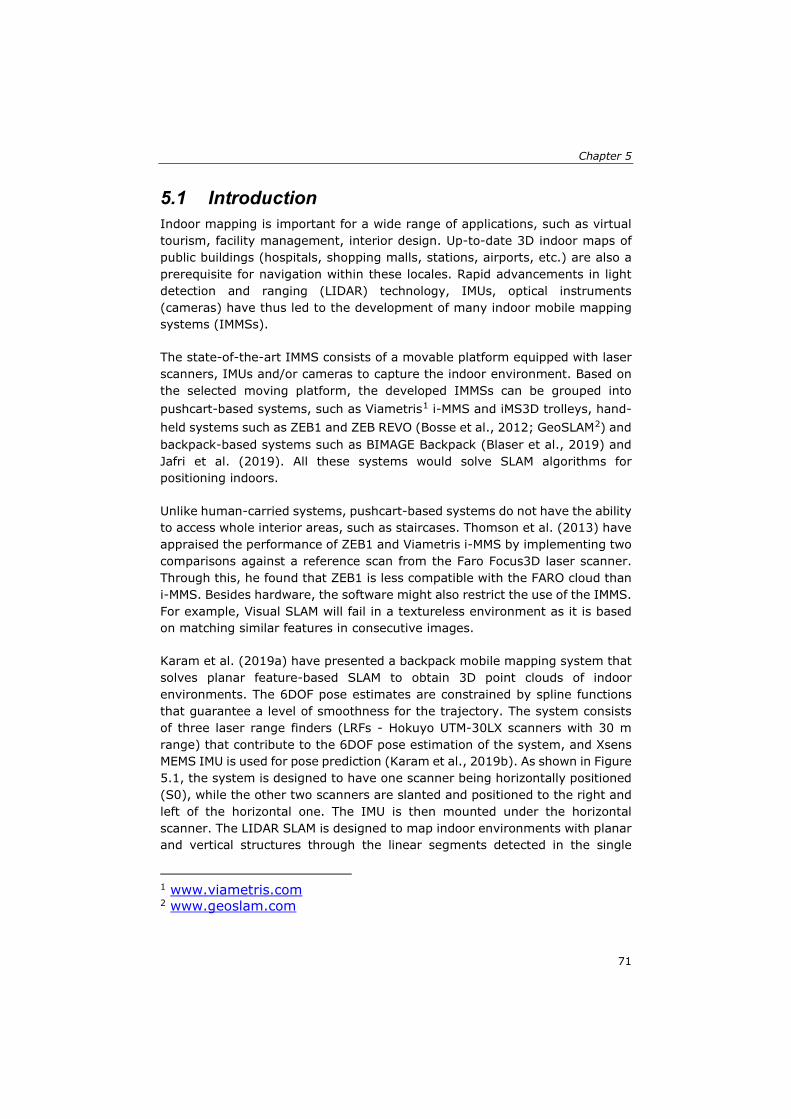
Chapter 5

71

5.1 Introduction Indoor mapping is important for a wide range of applications, such as virtual tourism, facility management, interior design. Up-to-date 3D indoor maps of public buildings (hospitals, shopping malls, stations, airports, etc.) are also a prerequisite for navigation within these locales. Rapid advancements in light detection and ranging (LIDAR) technology, IMUs, optical instruments (cameras) have thus led to the development of many indoor mobile mapping systems (IMMSs). The state-of-the-art IMMS consists of a movable platform equipped with laser scanners, IMUs and/or cameras to capture the indoor environment. Based on the selected moving platform, the developed IMMSs can be grouped into pushcart-based systems, such as Viametris1 i-MMS and iMS3D trolleys, hand-held systems such as ZEB1 and ZEB REVO (Bosse et al., 2012; GeoSLAM2) and backpack-based systems such as BIMAGE Backpack (Blaser et al., 2019) and Jafri et al. (2019). All these systems would solve SLAM algorithms for positioning indoors. Unlike human-carried systems, pushcart-based systems do not have the ability to access whole interior areas, such as staircases. Thomson et al. (2013) have appraised the performance of ZEB1 and Viametris i-MMS by implementing two comparisons against a reference scan from the Faro Focus3D laser scanner. Through this, he found that ZEB1 is less compatible with the FARO cloud than i-MMS. Besides hardware, the software might also restrict the use of the IMMS. For example, Visual SLAM will fail in a textureless environment as it is based on matching similar features in consecutive images. Karam et al. (2019a) have presented a backpack mobile mapping system that solves planar feature-based SLAM to obtain 3D point clouds of indoor environments. The 6DOF pose estimates are constrained by spline functions that guarantee a level of smoothness for the trajectory. The system consists of three laser range finders (LRFs - Hokuyo UTM-30LX scanners with 30 m range) that contribute to the 6DOF pose estimation of the system, and Xsens MEMS IMU is used for pose prediction (Karam et al., 2019b). As shown in Figure 5.1, the system is designed to have one scanner being horizontally positioned (S0), while the other two scanners are slanted and positioned to the right and left of the horizontal one. The IMU is then mounted under the horizontal scanner. The LIDAR SLAM is designed to map indoor environments with planar and vertical structures through the linear segments detected in the single

1 www.viametris.com 2 www.geoslam.com

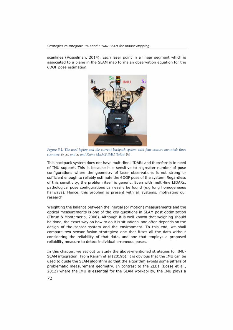
Strategies to Integrate IMU and LIDAR SLAM for Indoor Mapping

72

scanlines (Vosselman, 2014). Each laser point in a linear segment which is associated to a plane in the SLAM map forms an observation equation for the 6DOF pose estimation.

Figure 5.1. The used laptop and the current backpack system with four sensors mounted: three scanners S0, S1, and S2 and Xsens MEMS IMU (below S0)

This backpack system does not have multi-line LIDARs and therefore is in need of IMU support. This is because it is sensitive to a greater number of pose configurations where the geometry of laser observations is not strong or sufficient enough to reliably estimate the 6DOF pose of the system. Regardless of this sensitivity, the problem itself is generic. Even with multi-line LIDARs, pathological pose configurations can easily be found (e.g long homogeneous hallways). Hence, this problem is present with all systems, motivating our research. Weighting the balance between the inertial (or motion) measurements and the optical measurements is one of the key questions in SLAM post-optimization (Thrun & Montemerlo, 2006). Although it is well-known that weighing should be done, the exact way on how to do it is situational and often depends on the design of the sensor system and the environment. To this end, we shall compare two sensor fusion strategies: one that fuses all the data without considering the reliability of that data, and one that employs a proposed reliability measure to detect individual erroneous poses. In this chapter, we set out to study the above-mentioned strategies for IMU-SLAM integration. From Karam et al (2019b), it is obvious that the IMU can be used to guide the SLAM algorithm so that the algorithm avoids some pitfalls of problematic measurement geometry. In contrast to the ZEB1 (Bosse et al., 2012) where the IMU is essential for the SLAM workability, the IMU plays a

Chapter 5

73

supportive role in our SLAM. However, the big question is whether the IMU observations can be used also in the (final) pose estimation so that (1) pathological pose configurations are overcome and (2) the effect of IMU’s own drift to the pose estimates remains negligible. We answer to these very questions by proposing a combination of (1) a reliability measure for pose estimates derived from LIDAR observations and (2) coordinate and known-velocity updates, which reset the IMU drift. This resetting technique does not require a specific data capture mode to eliminate the IMU drifts as it is the case with the well-known Zero Velocity Updates (ZUPTs) technique (Chow et al., 2014). The remainder of this chapter is organized as follows: Section 5.2 presents the related works, while Section 5.3 describes our proposed strategies to integrate the IMU with LIDAR into SLAM after a short explanation of the IMU-less SLAM. In Section 5.4, we present results and discuss limitations of our approaches. The chapter ends with conclusions in Section 5.5. 5.2 Related Work Studies show IMU integration to increase the robustness of SLAM regardless of the type of the optical sensor. Many works tend to use LIDAR SLAM algorithms that incorporate one or more scanners in the pose estimation. NavVis1, for example, provided several solutions to map indoors as a trolley-based mobile mapping system that consisted mainly of scanners, IMUs and cameras. GeoSLAM company evolved several versions of the hand-held ZEB-scanner such as ZEB-REVO, ZEB-REVO RT, and ZEB Horizon. Besides the trolley-based and hand-held systems, there are several backpack systems (Lehtola et al., 2017). The Würzburg Backpack incorporates a 3D scanner (RIEGL VZ400), a 2D scanner (SICK LMS100) and an IMU that was utilized in the initial trajectory estimation (Lauterbach et al., 2015). Their experimental results showed maximum error about 7º in orientation and 25 cm in positioning. Zhang et al. (2017) attached an IMU to a LIDAR system to estimate odometry in real-time. All their walking experiments show that this combination improves the accuracy of motion estimation (See Table 3 in Zhang et al., 2017). The MEMS IMU in BIMAGE system, a component that combines two Velodyne VLP-16 laser scanners and one panorama camera, was exploited to estimate the camera orientation (Blaser et al., 2019). They solved 3D LIDAR SLAM for the Cartographer that combines the laser and IMU data, and then applied an image-based georeferencing approach to improve the camera pose estimation. Chow et al. (2014) integrated a MEMS IMU in their stop-and-go mobile mapping system (Scannect) to support the vision-based localization in case

1 www.navvis.com

Strategies to Integrate IMU and LIDAR SLAM for Indoor Mapping

74

the scene lacks features to be matched. They captured the data in a stop-and-go movement mode in order to utilize ZUPTs to eliminate the IMU drifts. 5.3 IMU-SLAM Integration Strategies As the backpack system is a mobile and multi-sensor system, we defined two main coordinate systems. The frame system (f) which is constantly moving and the data of all sensors are registered in it. The model system (m) which is a fixed system and used to register the moving frame system over time. The final point clouds are defined in this system as well. In our planar feature-based SLAM, we modelled the frame 6DOF pose parameters (X, Y, Z, ω, ϕ, κ) in the model coordinate system (m) as functions of time using splines, and the planes were modelled by the normal vector and distance to the origin. The coefficients of the pose splines and the plane parameters are estimated simultaneously (Karam et al., 2019a). Thus, the adjustment process within SLAM does not only estimate and update the pose parameters but also the planes, which goes through different stages, as listed below. Figure 5.2 illustrates these stages exemplary. The differences between these stages are the splines’ order, parameters to estimate, and the number of scans involved. • Local adjustment: runs over a few successive scans captured during 0.1 s or slightly longer, and relies on the pose predicted by the IMU to check data association between the newly captured points and the previously reconstructed planes (Karam et al., 2019b). Each assigned point forms a laser observation equation and participates in the estimation of pose parameters that are modelled using linear splines. The laser observation equation is formulated based on the expectation that the distance between a point and its associated plane, i.e., plane that the point belongs to, equals zero. See Vosselman (2014) for details. The pose parameters are estimated and updated in this adjustment, while parameters of earlier instantiated planes are kept fixed. • IMU-based prediction: runs at the beginning of each local adjustment to test the data association as mentioned above. Here, we utilized the strength of the IMU in short-term pose prediction and we predicted the pose within a time window that covers the time interval of one scan (25 ms). The IMU drifts are reset at the start time of each prediction window by using the position and the approximate velocity of the system estimated from the previous local adjustment at that time. Then, using the IMU data taken within this window, we predict the pose of the next scan (Karam et al., 2019b).

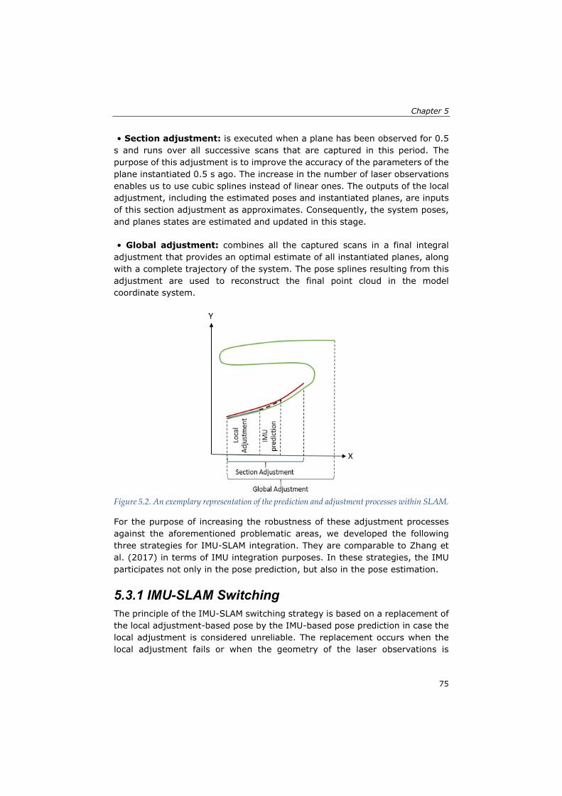
Chapter 5

75

• Section adjustment: is executed when a plane has been observed for 0.5 s and runs over all successive scans that are captured in this period. The purpose of this adjustment is to improve the accuracy of the parameters of the plane instantiated 0.5 s ago. The increase in the number of laser observations enables us to use cubic splines instead of linear ones. The outputs of the local adjustment, including the estimated poses and instantiated planes, are inputs of this section adjustment as approximates. Consequently, the system poses, and planes states are estimated and updated in this stage. • Global adjustment: combines all the captured scans in a final integral adjustment that provides an optimal estimate of all instantiated planes, along with a complete trajectory of the system. The pose splines resulting from this adjustment are used to reconstruct the final point cloud in the model coordinate system.

Figure 5.2. An exemplary representation of the prediction and adjustment processes within SLAM.

For the purpose of increasing the robustness of these adjustment processes against the aforementioned problematic areas, we developed the following three strategies for IMU-SLAM integration. They are comparable to Zhang et al. (2017) in terms of IMU integration purposes. In these strategies, the IMU participates not only in the pose prediction, but also in the pose estimation. 5.3.1 IMU-SLAM Switching The principle of the IMU-SLAM switching strategy is based on a replacement of the local adjustment-based pose by the IMU-based pose prediction in case the local adjustment is considered unreliable. The replacement occurs when the local adjustment fails or when the geometry of the laser observations is

Strategies to Integrate IMU and LIDAR SLAM for Indoor Mapping

76

insufficient to estimate the pose. We decide whether or not to switch to the IMU-based estimate based on several indicators that measure the reliability of the SLAM-based estimate. The first indicator is the reciprocal condition number (rcond) of the normal matrix, which tells how close/far the normal matrix is to being singular. A very small rcond indicates that the normal matrix is close to being singular or badly scaled. Another indicator of a poor conditioned equation system is a high correlation between the estimated parameters. We determined the correlation matrix and check the maximum absolute value of all non-diagonal elements. If this value is approaching 1 for any pair of parameters, these parameters are highly correlated and it would, therefore, be hard to determine them separately. In addition, we added a well-known scan matching technique, iterative closest points (ICP), to the proposed method. This technique is commonly used as a pose estimation method to support SLAM by defining the relative transformation between successive scans (Lee et al., 2011). We utilized the strength and efficiency of 2D ICP in estimating the relative 2D transformation (X, Y, κ) when it matches two successive scans of the horizontally mounted scanner. As the time interval of one scan is 25 ms, a large rotation between two scans in this short period is not expected. However, we would not rely on the 3DOF ICP-based pose to move forward in SLAM. Rather, we are simply determining the differences in the estimated pose parameters (X, Y, k) between the ICP and local adjustment. A big difference would raise the suspicion that one of the two methods is wrong, and this is used as an indicator to switch to the IMU-based prediction. 5.3.2 IMU-based Pose Estimation The difference with the switching technique is that we always use the IMU-based pose prediction instead of the local adjustment-based pose, no matter whether the local adjustment seems reliable or not. The role of the local adjustment is limited to instantiate planes and for the checking of data association. 5.3.3 IMU-SLAM Joint Estimation In this strategy, we deepen the SLAM-IMU integration by including the IMU observations in the 6DOF pose estimation besides the laser observations. Our Xsens MEMS IMU measures three-dimensional angular velocity and three-dimensional dynamic acceleration over time. Some of our IMU specifications are listed in Table 5.1. Similar to Hussnain et al. (2018), we formulate six IMU observation equations at each timestamp, 𝑡𝑡, as described in the following subsections.

Chapter 5

77

Table 5.1. Key specifications of the Xsens MEMS IMU

SLAM Gyroscope Accelerometer

Bias repeatability 0.2º/s 0.03 m/s2

In-run bias stability 10º/h 40 μg

5.3.3.1 Acceleration Observation Equations The IMU accelerometers observe the accelerations �̈�𝑇𝑖𝑖𝑚𝑚𝑖𝑖𝑠𝑠 = (�̈�𝑑𝑖𝑖𝑚𝑚𝑖𝑖s , �̈�𝑑𝑖𝑖𝑚𝑚𝑖𝑖s , �̈�𝑑𝑖𝑖𝑚𝑚𝑖𝑖𝑠𝑠 ) in the sensor coordinate system (s) which needs to be rotated to the frame coordinate system (f) with the time-independent rotation matrix 𝑅𝑅𝑠𝑠

𝑓𝑓 = 𝑅𝑅𝑧𝑧(90). This will also need to be performed on the model system (m) with the time-dependent rotation matrix 𝑅𝑅𝑓𝑓𝑚𝑚(𝜔𝜔,𝜑𝜑, 𝜅𝜅). Hence,

�̈�𝑇𝑖𝑖𝑚𝑚𝑖𝑖𝑚𝑚 = 𝑅𝑅f𝑚𝑚 𝑅𝑅𝑠𝑠

𝑓𝑓 �̈�𝑇𝑖𝑖𝑚𝑚𝑖𝑖𝑠𝑠 (5.1)

As the resulting accelerations (�̈�𝑇𝑖𝑖𝑚𝑚𝑖𝑖𝑚𝑚 ) should correspond to the second-order derivative of the backpack’s location (�̈�𝑇𝑓𝑓𝑚𝑚) in the model system, the following observation equations are formulated:

�̈�𝑇𝑓𝑓𝑚𝑚 = 𝑅𝑅𝑓𝑓𝑚𝑚 𝑅𝑅𝑠𝑠𝑓𝑓 �̈�𝑇𝑖𝑖𝑚𝑚𝑖𝑖

𝑠𝑠 − �00𝑔𝑔� (5.2)

where �̈�𝑇𝑓𝑓𝑚𝑚 = (�̈�𝑑𝑓𝑓m, �̈�𝑑𝑓𝑓m, �̈�𝑑𝑓𝑓𝑚𝑚). Since the z-axis in the model system is assumed to be vertical, we compensate for the effect of gravity in the accelerometer reading by subtracting the average gravitational acceleration (𝑔𝑔) from the acceleration along this axis. As the pose parameters are modelled using splines in the laser observation equations, we also modelled the accelerations using splines. Splines are polynomial functions and it is straightforward to derive the accelerations (�̈�𝑇𝑓𝑓𝑚𝑚) as the second-order derivatives of the translations (𝑇𝑇𝑓𝑓𝑚𝑚). For example, for the translation 𝑑𝑑 spline 𝑑𝑑(𝑡𝑡) = ∑ 𝛼𝛼𝑥𝑥,𝑖𝑖 𝐵𝐵𝑖𝑖(𝑡𝑡)𝑖𝑖 , the acceleration �̈�𝑑 spline becomes �̈�𝑑(𝑡𝑡) =∑ 𝛼𝛼𝑥𝑥,𝑖𝑖 �̈�𝐵𝑖𝑖(𝑡𝑡)𝑖𝑖 , where 𝛼𝛼𝑥𝑥,𝑖𝑖 is the 𝑑𝑑 spline coefficient to be estimated on interval 𝑖𝑖. Hence, both the translations and accelerations are expressed in terms of the same to-be-determined spline coefficients.

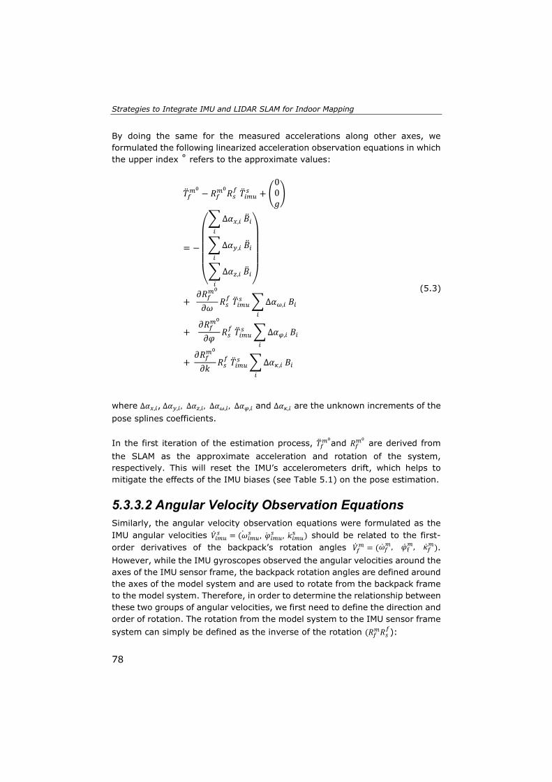
Strategies to Integrate IMU and LIDAR SLAM for Indoor Mapping

78

By doing the same for the measured accelerations along other axes, we formulated the following linearized acceleration observation equations in which the upper index ˚ refers to the approximate values:

�̈�𝑇𝑓𝑓𝑚𝑚0 − 𝑅𝑅𝑓𝑓𝑚𝑚

0𝑅𝑅𝑠𝑠𝑓𝑓 �̈�𝑇𝑖𝑖𝑚𝑚𝑖𝑖𝑠𝑠 + �

00𝑔𝑔�

= −

⎝

⎜⎜⎜⎛�Δ𝛼𝛼𝑥𝑥,𝑖𝑖 �̈�𝐵𝑖𝑖𝑖𝑖

�Δ𝛼𝛼𝑦𝑦,𝑖𝑖 �̈�𝐵𝑖𝑖𝑖𝑖

�Δ𝛼𝛼𝑧𝑧,𝑖𝑖 �̈�𝐵𝑖𝑖𝑖𝑖 ⎠

⎟⎟⎟⎞

+ 𝜕𝜕𝑅𝑅𝑓𝑓𝑚𝑚

0

𝜕𝜕𝜔𝜔𝑅𝑅𝑠𝑠𝑓𝑓 �̈�𝑇𝑖𝑖𝑚𝑚𝑖𝑖

𝑠𝑠 �Δ𝛼𝛼𝜔𝜔,𝑖𝑖 𝐵𝐵𝑖𝑖𝑖𝑖

+ 𝜕𝜕𝑅𝑅𝑓𝑓𝑚𝑚

0

𝜕𝜕𝜑𝜑𝑅𝑅𝑠𝑠𝑓𝑓 �̈�𝑇𝑖𝑖𝑚𝑚𝑖𝑖𝑠𝑠 �Δ𝛼𝛼𝜑𝜑,𝑖𝑖 𝐵𝐵𝑖𝑖

𝑖𝑖

+ 𝜕𝜕𝑅𝑅𝑓𝑓𝑚𝑚

0

𝜕𝜕𝜕𝜕𝑅𝑅𝑠𝑠𝑓𝑓 �̈�𝑇𝑖𝑖𝑚𝑚𝑖𝑖𝑠𝑠 �Δ𝛼𝛼𝜅𝜅,𝑖𝑖 𝐵𝐵𝑖𝑖

𝑖𝑖

(5.3)

where Δ𝛼𝛼𝑥𝑥,𝑖𝑖, Δ𝛼𝛼𝑦𝑦,𝑖𝑖 , Δ𝛼𝛼𝑧𝑧,𝑖𝑖 , Δ𝛼𝛼𝜔𝜔,𝑖𝑖 , Δ𝛼𝛼𝜑𝜑,𝑖𝑖 and Δ𝛼𝛼𝜅𝜅,𝑖𝑖 are the unknown increments of the pose splines coefficients. In the first iteration of the estimation process, �̈�𝑇𝑓𝑓𝑚𝑚

0and 𝑅𝑅𝑓𝑓𝑚𝑚0 are derived from

the SLAM as the approximate acceleration and rotation of the system, respectively. This will reset the IMU’s accelerometers drift, which helps to mitigate the effects of the IMU biases (see Table 5.1) on the pose estimation. 5.3.3.2 Angular Velocity Observation Equations Similarly, the angular velocity observation equations were formulated as the IMU angular velocities �̇�𝑉𝑖𝑖𝑚𝑚𝑖𝑖𝑠𝑠 = (�̇�𝜔𝑖𝑖𝑚𝑚𝑖𝑖

𝑠𝑠 , �̇�𝜑𝑖𝑖𝑚𝑚𝑖𝑖𝑠𝑠 , �̇�𝜅𝑖𝑖𝑚𝑚𝑖𝑖s ) should be related to the first-order derivatives of the backpack’s rotation angles �̇�𝑉𝑓𝑓𝑚𝑚 = (�̇�𝜔𝑓𝑓𝑚𝑚, �̇�𝜑f𝑚𝑚, �̇�𝜅𝑓𝑓𝑚𝑚). However, while the IMU gyroscopes observed the angular velocities around the axes of the IMU sensor frame, the backpack rotation angles are defined around the axes of the model system and are used to rotate from the backpack frame to the model system. Therefore, in order to determine the relationship between these two groups of angular velocities, we first need to define the direction and order of rotation. The rotation from the model system to the IMU sensor frame system can simply be defined as the inverse of the rotation (𝑅𝑅𝑓𝑓𝑚𝑚𝑅𝑅𝑠𝑠

𝑓𝑓):

Chapter 5

79

𝑅𝑅𝑚𝑚s = (𝑅𝑅f𝑚𝑚𝑅𝑅𝑠𝑠

𝑓𝑓)𝑇𝑇 = 𝑅𝑅𝑓𝑓𝑠𝑠𝑅𝑅𝑚𝑚𝑓𝑓 =

𝑅𝑅𝑓𝑓𝑠𝑠 𝑅𝑅3�𝜅𝜅𝑓𝑓𝑚𝑚�𝑇𝑇𝑅𝑅2�𝜑𝜑𝑓𝑓𝑚𝑚�

𝑇𝑇𝑅𝑅1�ω𝑓𝑓𝑚𝑚�𝑇𝑇

(5.4)

As κ is the first rotation applied when rotating from the backpack frame to the model system, the angular velocity around the z-axis (�̇�𝜅𝑓𝑓𝑚𝑚) would not have to

be rotated by 𝑅𝑅𝑚𝑚𝑓𝑓 (Karam et al., 2019b). Indeed the IMU angular velocity �̇�𝜑𝑖𝑖𝑚𝑚𝑖𝑖s

around the y-axis does not hold a direct correspondence with the first derivative of 𝜑𝜑𝑓𝑓𝑚𝑚 when simply rotating (𝑅𝑅𝑓𝑓𝑆𝑆) from the backpack frame to the IMU sensor system. This is as the y-axis has already been rotated by −𝜅𝜅𝑓𝑓𝑚𝑚 around the z-axis prior to the measuring of �̇�𝜑𝑖𝑖𝑚𝑚𝑖𝑖s in the IMU sensor system. As such, the derivative of 𝜑𝜑𝑓𝑓𝑚𝑚 should also be rotated to the frame system. Similarly, the derivative of 𝜔𝜔𝑓𝑓𝑚𝑚 would need to be rotated by −𝜑𝜑𝑓𝑓𝑚𝑚 around the y-axis, and by −𝜅𝜅𝑓𝑓𝑚𝑚 around the z-axis, in order to obtain an angular velocity vector in the frame system. Hence, after rotating from the frame system to the IMU system, we were able to obtain the angular velocities as defined by the pose splines in the IMU system. This leads to the following observation equations:

��̇�𝜔𝑖𝑖𝑚𝑚𝑖𝑖𝑠𝑠

�̇�𝜑𝑖𝑖𝑚𝑚𝑖𝑖𝑠𝑠

�̇�𝜅𝑖𝑖𝑚𝑚𝑖𝑖𝑠𝑠� = 𝑅𝑅𝑓𝑓𝑆𝑆 �

00�̇�𝜅𝑓𝑓𝑚𝑚

� + 𝑅𝑅𝑓𝑓𝑆𝑆𝑅𝑅3�𝜅𝜅𝑓𝑓𝑚𝑚�𝑇𝑇 �

0�̇�𝜑f𝑚𝑚0�

+ 𝑅𝑅𝑓𝑓𝑆𝑆𝑅𝑅3�𝜅𝜅𝑓𝑓𝑚𝑚�𝑇𝑇𝑅𝑅2�𝜑𝜑𝑓𝑓𝑚𝑚�

𝑇𝑇 ��̇�𝜔𝑓𝑓m

00�

(5.5)

It can be shortened to:

�̇�𝑉𝑖𝑖𝑚𝑚𝑖𝑖𝑠𝑠 = 𝑅𝑅𝑓𝑓𝑆𝑆𝑆𝑆𝑚𝑚𝑓𝑓 �̇�𝑉𝑓𝑓𝑚𝑚 (5.6)

with 𝑆𝑆𝑚𝑚𝑓𝑓 = �

cos𝜑𝜑 cos𝜅𝜅 sin𝜅𝜅 0− cos𝜑𝜑 sin𝜅𝜅 cos𝜅𝜅 0

sin𝜑𝜑 0 1�𝑚𝑚

𝑓𝑓

where 𝑆𝑆𝑚𝑚

𝑓𝑓 is the transformation matrix from the model to the frame system. We model the angular velocities using splines as well by taking first-order derivatives of the rotation angles. For instance, for the rotation angle ω spline ω(𝑡𝑡) = ∑ 𝛼𝛼𝜔𝜔,𝑖𝑖 𝐵𝐵𝑖𝑖(𝑡𝑡)𝑖𝑖 , the angular velocity �̇�𝜔 spline becomes �̇�𝜔(𝑡𝑡) = ∑ 𝛼𝛼𝜔𝜔,𝑖𝑖 �̇�𝐵𝑖𝑖(𝑡𝑡)𝑖𝑖 , where 𝛼𝛼𝜔𝜔,𝑖𝑖 is the ω spline coefficient to be estimated on interval 𝑖𝑖. Hence, the linearized angular velocity observation equations become:

Strategies to Integrate IMU and LIDAR SLAM for Indoor Mapping

80

�̇�𝑉𝑖𝑖𝑚𝑚𝑖𝑖𝑠𝑠 − 𝑅𝑅𝑓𝑓𝑠𝑠𝑆𝑆𝑚𝑚𝑓𝑓 0�̇�𝑉𝑓𝑓𝑚𝑚

0

= 𝑅𝑅𝑓𝑓𝑠𝑠𝑆𝑆𝑚𝑚𝑓𝑓 0

⎝

⎜⎜⎜⎛�Δ𝛼𝛼𝜔𝜔,𝑖𝑖 �̇�𝐵𝑖𝑖(𝑡𝑡)𝑖𝑖

�Δ𝛼𝛼𝜑𝜑,𝑖𝑖 �̇�𝐵𝑖𝑖(𝑡𝑡)𝑖𝑖

�Δ𝛼𝛼𝜅𝜅,𝑖𝑖 �̇�𝐵𝑖𝑖(𝑡𝑡)𝑖𝑖 ⎠

⎟⎟⎟⎞

+ 𝑅𝑅𝑓𝑓𝑠𝑠𝜕𝜕𝑆𝑆𝑚𝑚

𝑓𝑓 0

𝜕𝜕𝜕𝜕�̇�𝑉𝑓𝑓𝑚𝑚

0�Δ𝛼𝛼𝑘𝑘,𝑖𝑖 𝐵𝐵𝑖𝑖𝑖𝑖

+ 𝑅𝑅𝑓𝑓𝑠𝑠𝜕𝜕𝑆𝑆𝑚𝑚

𝑓𝑓 0

𝜕𝜕𝜑𝜑�̇�𝑉𝑓𝑓𝑚𝑚

0�Δ𝛼𝛼𝜑𝜑,𝑖𝑖 𝐵𝐵𝑖𝑖𝑖𝑖

(5.7)

Similar to the acceleration equation, the angular velocities �̇�𝑉𝑓𝑓𝑚𝑚

0 and the

transformation matrix 𝑆𝑆𝑚𝑚𝑓𝑓 0 in the first iteration of the estimation process are

derived from the approximate splines. This helps to reset the IMU’s gyroscope drift and this, in turn, eliminates the attitude drift considerably. 5.3.3.3 Joint Estimation For the joint estimation method, the IMU observation equations (Eq. (5.3) and Eq. (5.7)) are added to the laser observation equations in all adjustment processes addressed above: local, section and global. This fusion enables us to use cubic splines instead of linear ones in the local adjustment. As our backpack system was mounted with three Hokuyo scanners with a scanning frequency of 40 Hz and 1080 points per scan line, every 25 ms the system records 3240 laser points. The accelerations and angular velocities are recorded by the IMU with a sampling frequency of 200 Hz; thus, for a local adjustment within 0.1 s, we have 12960 laser points, 60 IMU acceleration readings, and 60 IMU angular velocity readings. However, not all laser points were assigned to planes and can contribute to the pose estimation, as this is based on the data association criteria. 5.4 Experimental Results and Discussion In order to test the performance of the three proposed strategies for a SLAM-IMU integration, several experiments on different indoor environments were conducted. Three datasets were collected at the Institute of Geodesy and Photogrammetry building at the University of Braunschweig, Germany. They are denoted Diemen0, Diemen1, and Diemen2, respectively. The number of captured laser points and the walking duration for all test areas are approximately 38 million/5-minute, 73 million/9-minute, and 38 million/5-

Chapter 5

81

minute, respectively. Diemen0 is captured in the relatively cluttered basement, while the other two datasets are captured on the ground floor with different operators and trajectories. The mapped areas show distinct office environments that have plenty of doors and windows. There were also several narrow rooms with glass windows and uneven curtains. In order to test for the aforementioned weaknesses, some doors were wide open, and others were opened by the operator while the data was being captured. As the rooms in Diemen1 and Diemen2 were nearly empty due to renovation works, the number of planar structures is limited. This, in turn, affected the estimability of the system pose using only laser observations. The previously mentioned features of the test areas sometimes constitute as obstacles, and this may cause some of previously developed LIDAR SLAMs to fail before the mapping was completed, see Table 5.3. We mapped these test areas using our backpack indoor mobile mapping system and ran five different versions of SLAM algorithms on each dataset. For the IMU-SLAM Switching, the rcond and correlation thresholds are experimentally determined and set to 0.02 and 0.7, respectively. The differences thresholds with ICP to raise the suspicion in SLAM performance are set to 1 cm for (x, y), and 0.5º for k. For the purpose of simplicity, we use the following terminology for the five compared SLAM strategies; LIDAR SLAM: relies on the linear extrapolation for pose prediction instead of the IMU (Karam et al., 2019a). LIDAR SLAM with IMU prediction: takes advantage of the IMU to predict the next pose (Karam et al., 2019b). IMU-SLAM Switching, IMU-based Pose Estimation, and IMU-SLAM Joint Estimation are the three IMU-SLAM integration techniques proposed in this chapter (see Table 5.2). Table 5.2. Comparison between the proposed methods in this chapter and previously developed methods regarding the data source for pose prediction and estimation.

SLAM Algorithm 6DOF Pose prediction

6DOF Pose estimation

LIDAR SLAM (Karam et al., 2019a) LIDAR LIDAR

LIDAR SLAM (Karam et al., 2019b) LIDAR+IMU LIDAR

Three methods proposed in this chapter LIDAR+IMU LIDAR+IMU

The most crucial aspect in the testing of the proposed methods was to check the robustness against poor laser observation geometries. Indeed, the

Strategies to Integrate IMU and LIDAR SLAM for Indoor Mapping

82

improvement in terms of robustness was evident through the ability to handle more datasets. This is particularly evident for the Diemen1 data, which the LIDAR SLAM, even with the help of IMU prediction, failed to process, as shown in Table 5.3. While for the Diemen0 data, all methods that estimate the pose without the use of IMU observations failed. This failure is caused by the divergence of the global adjustment because of insufficient laser observations in a sequence of five or more intervals. Figure 5.3 shows an obvious case where the LIDAR SLAM fails without the support of an IMU. There is an insufficient amount of laser observations to estimate the translation along the Y-axis. Therefore, the system slides along the Y-axis and leads to an erroneous map. One reason for the poor laser observations is that the narrow wall in front of the operator has a large transparent object (glass window), which leads to missing or incorrect range measurements. Problematic areas also include a non-flat panel radiator underneath the window and a winding curtain reflect in sparse laser scans in which it is hard to detect linear segments. There are also no observations on the wall at the opposite side of the room because of the 270º opening angle of the Hokuyo scanners. In comparison to the other methods, the IMU-SLAM joint estimation is the most robust method due to its ability to handle all datasets in this chapter. The reliance on IMU allows the SLAM to reconnect to planes seen some longer time before; thus, this prevents the system from sliding in any direction and supports the SLAM in going ahead.

(a)

(b)

Figure 5.3. An example of a problematic area for the LIDAR SLAM. a) 3D reconstructed planes (black) with the assigned laser points from four scans (colours indicate point associations to a particular plane) and the points that are not associated to a plane (red). The arrow refers to the Y-axis direction in the model system. b) The wall is in front of the operator.

We performed a comparison between the resulting point clouds (Figure 5.4) based on several factors, such as the number of points assigned to the reconstructed planes and the root mean square error (RMSE) of the residuals,

Chapter 5

83

as demonstrated in Table 5.3. In this chapter, the term residuals refers to the distances between the model planes and the points associated to them. Table 5.3 demonstrates that the use of IMU in pose estimation has increased significantly the number of assigned points to planes in Diemen2 dataset from about 24 million points to 28 million points. Approximately 97% of the assigned points have residuals below 3 cm, which is 10% higher than in the case of not using the IMU. Also, the RMSE of the residuals decreased from 1.8 cm with LIDAR SLAM to about 1.3 cm. Consequently, the proposed strategies for IMU integration lead into a more robust data association between the captured points and the reconstructed planes. As the SLAM-IMU joint estimation tries to fit the trajectory to the IMU observations, it is slightly sacrificing the minimization of the point-to-plane distances. Therefore, Table 5.3 shows that this method is not always the best performing method regarding the RMSE of residuals, even if it is the most robust method. Figure 5.5 compares the histograms of the points’ residuals of all resulting point clouds for the Diemen2 dataset as it is the only dataset that was processed successfully by all methods. It demonstrates that approximately 57% of the assigned points have residuals below 1 cm when the IMU was not used at all. This improved to 61% when the switching technique took place, to 64% when the IMU was utilized in pose prediction and to about 70% when IMU contributes to the pose estimation. On the other hand, approximately 13% of the residuals exceeded 3 cm when the IMU was not used. This percentage is negligible when the IMU is utilized for pose prediction and estimation. As such, this is why the RMSE value of the assigned points’ residuals decreases (Table 5.3). However, the previous measurements, the number of assigned points and the RMSE of their residuals, do not adequately reflect the overall quality of the methods’ performance. The lower RMSE indicates that we do a better fit of points to planes, but this does not necessarily mean that we have a better model. In addition, the RMSE could be influenced badly by an incorrect merge of two planes. Therefore, we applied further quality measures which utilized the architectural constraints of walls (perpendicularity and parallelism) as they are predominant characteristics in the scanned areas (Karam et al., 2018). We assessed the ability of the system to capture the true geometry of the scanned environment. The results in Table 5.4 show the reconstruction accuracy with the IMU contribution is much better than without IMU. The percentages of small angles’ errors (<0.5º) increase and outliers (>1º) decrease in all the proposed methods that utilize the IMU.

Strategies to Integrate IMU and LIDAR SLAM for Indoor Mapping

84

(a) Diemen0

(b) Diemen2

(c) Diemen1

Figure 5.4. The generated point cloud of the test areas with colours show plane association and trajectory followed (white). For visualization purposes, the points that are not associated to a plane and the points on the ceiling are removed from the point clouds.

Chapter 5

85

Table 5.3. Comparison between the performance of the proposed method on all datasets regarding the number of assigned points (Nr), the corresponding RMSEs of the residuals, and the percentage of residuals below 3 cm (Perc). The results of two previously developed methods are also listed at the beginning of the table for comparison. The letter “x” refers to the failure of the method to process the corresponding dataset.

Dataset SLAM Diemen0 Diemen1 Diemen2

LIDAR SLAM (Karam et al., 2019a)

Nr (million) x

x

24 RMSE (cm) 1.8

Perc (%) 87

LIDAR SLAM (Karam et al., 2019b)

Nr (million) x

x

24 RMSE (cm) 1.3

Perc (%) 96

IMU-SLAM switching Nr (million)

x

53 28 RMSE (cm) 1.5 1.4

Perc (%) 96 97

IMU-based Pose Estimation

Nr (million) x

53 28 RMSE (cm) 1.8 1.4

Perc (%) 96 97

IMU-SLAM Joint Estimation

Nr (million) 28 53 28 RMSE (cm) 1.5 1.6 1.3

Perc (%) 98 96 97

Figure 5.5. Histograms of the points’ residuals of all resulting point clouds for Diemen2 dataset and for all methods, LIDAR SLAM (black), with IMU prediction (red), IMU-SLAM switching (magenta), IMU-based Pose Estimation (blue), and the joint estimation (green).

0 5

0

20

40

60

80

Perc

enta

ge [%

]

0 5 0 5

Residual [cm]

0 5 0 5

Strategies to Integrate IMU and LIDAR SLAM for Indoor Mapping

86

Table 5.4. Comparison between the performance of the proposed method on all datasets regarding the architectural constraints. The percentages of angles’ errors in three different ranges for parallelism (par) and perpendicularity (perp) and the corresponding RMSEs. The results of two previously developed methods are also listed at the beginning of the table for comparison. The letter “x” refers to the failure of the method to process the corresponding dataset.

Dataset SLAM

Diemen0 Diemen1 Diemen2 perp par perp par Perp par

LIDAR SLAM (Karam et al., 2019a)

[0º 0.5º[

x x

58 50 [0.5º 1º] 26 12 [1º 5º] 16 38

RMSE (deg) 1.34º 1.76º

LIDAR SLAM (Karam et al., 2019b)

[0º 0.5º[

x x

70 66 [0.5º 1º] 23 13 [1º 5º] 7 21

RMSE (deg) 0.66º 1.39º

IMU-SLAM Switching

[0º 0.5º[

x

69 62 67 65 [0.5º 1º] 19 16 23 16 [1º 5º] 12 22 10 19

RMSE (deg) 0.54º 1.31º 0.96º 1.50º

IMU-based Pose Estimation

[0º 0.5º[

x

68 54 70 71 [0.5º 1º] 17 16 23 11 [1º 5º] 15 30 7 18

RMSE (deg) 0.66º 1.36º 0.63º 1.06º

IMU-SLAM Joint Estimation

[0º 0.5º[ 62 39 67 57 67 61 [0.5º 1º] 25 30 18 16 23 12 [1º 5º] 13 31 15 27 10 27

RMSE (deg) 0.63º 1.34º 0.70º 1.45º 0.82º 1.46º

It also demonstrates that the reliance on the IMU at many locations did not negatively affect the internal consistency of walls; thus, it did not impede upon the correctness of the final 3D reconstruction. However, Table 5.4 shows that the best results were reached when the SLAM kept switching to the IMU. Overall, we observe an improvement in results when the erroneous poses that originate from LIDAR SLAM are replaced by the poses integrated from IMU measurements. This goes hand-in-hand with the general understanding that the less trustworthy measurements should receive no weight in SLAM optimization. The proposed SLAM strategies are limited to (indoor) environments with planar structures. The IMU drift in velocity and heading is reset in each prediction or estimation loop (see Section 5.3), but the IMU biases are not auto-calibrated

Chapter 5

87

during scanning. This did not cause immediate problems in our experiments but should be taken into account with lower quality IMUs. In this case, this limitation could be addressed, e.g., for the gyro biases (Hyyti and Visala, 2015). 5.5 Conclusions And Future Work We have described several strategies to integrate the IMU with the LIDAR SLAM. Here, the IMU participates in the pose prediction and estimation. We conclude that the IMU integration improves the robustness of both the data association and pose estimation and therefore it is beneficial in the proposed SLAM approach. This improvement in the SLAM robustness expands the scope of application of our backpack mobile mapping system. In future works, we intend to investigate whether the IMU is capable to generate a reliable prediction for a longer exposure period. Reliable prediction for a longer period will help to improve the hypothesis generation for planar structures, which in turn, enables the SLAM to sense non-vertical walls or non-horizontal floors/ceilings. Consequently, this would expand the applicability of our system.

Strategies to Integrate IMU and LIDAR SLAM for Indoor Mapping

88

89

Chapter 6 - Simple loop closing for continuous LIDAR&IMU Planar Graph SLAM for 3D indoor environments * 1

* This chapter is based on:

Karam, S., Lehtola, V., and Vosselman, G. (2021). Simple loop closing for continuous LIDAR&IMU Planar Graph SLAM for 3D indoor environments. ISPRS Journal of Photogrammetry and Remote Sensing (Accepted)

Simple loop closing for continuous LIDAR&IMU Planar Graph SLAM for 3D indoor environments

90

Abstract Simultaneous localization and mapping (SLAM) is the essential technique in mapping environments that are denied to the global navigation satellite systems (GNSSs), such as indoor spaces. In this article, we present a loop-closing continuous-time LIDAR-IMU SLAM for indoor environments. The design of the proposed SLAM is based on arbitrarily-oriented planar features that allow for point to plane matching for local but also global optimization. Moreover, to update the SLAM graph during the optimization, we propose a simple yet elegant loop closure method in the form of merging the planes together. Representing the SLAM map by planes is advantageous due to the abundant existence of planar structures in indoor built environments. The proposed method was validated on a specific configuration of three 2D LIDAR scanners mounted on a wearable platform (backpack). Scanned point clouds were compared against ones obtained from a commercial mobile mapping system (Viametris iMS3D) and a terrestrial laser scanner (RIEGL VZ-400). The experimental results demonstrate that our SLAM system is capable of mapping multi-storey buildings, staircases, cluttered areas and areas with curved walls. Furthermore, our SLAM system offers comparable performance to that of the commercial system as shown by the low deviation between the point clouds generated by both systems. The majority of the cloud-to-cloud absolute distances – about 92 % – are less than 3 cm.

Chapter 6

91

6.1 Introduction Three-dimensional (3D) digital models of indoor environments can be advantageous to professionals from various disciplines such as engineering, architecture and archaeology. Indoor mobile mapping systems (IMMSs) digitize indoor environments quickly and at high levels of detail (Lehtola et al. 2017; Maboudi et al., 2017). Such systems have advantages over terrestrial laser scanners (TLS) in terms of time-consumption and labour. The IMMSs rely on simultaneous localization and mapping (SLAM) algorithm for positioning in spaces and environments inaccessible to the global navigation satellite systems (GNSSs). The core idea of SLAM (Cadena et al., 2016) is to map unknown environments. In this task, problems arise from that these environments may contain pathological geometries and from that the platform motion may be erratic (Yu & Zhang, 2019). Specifically, light detection and ranging (LIDAR) SLAM degenerates in those pose configurations where the geometry of LIDAR observations is insufficient to estimate the 3D pose of the mapping system. In LIDAR-inertial measurement unit (IMU) SLAM (Geneva et al., 2018; Karam et al., 2020), the LIDAR provides accurate geometrical data, while the IMU prevents the SLAM from degenerating, for example, when the platform experiences fast rotations. Although the IMU sensor provides good short-term motion estimates (Karam et al., 2019; Yang et al., 2019), it suffers from accumulated errors over time due to the dead reckoning-based positioning, and therefore obviously is undesirable as a stand-alone sensor for positioning purposes. SLAM can be run online to estimate the current pose of a mapping system or offline to optimize an entire trajectory. In the first, only a part of the historic data is used to keep the computational load tractable for real time applications, see e.g., Kalman filter-based SLAMs (Ji et al., 2020; Lin et al., 2021). This is in contrast to the offline SLAM that optimizes the trajectory over the entire recorded data such as graph SLAM (Grisetti et al., 2010). Therefore, the offline SLAM is usually more accurate than the online SLAM. Accordingly, it is often used in mobile mapping where the geometric accuracy of the map is the most important factor. Typically, graph SLAM uses a discrete pose representation, i.e., it consists of nodes, representing the mapping system poses, connected by edges representing the sensors’ measurements that constrain the connected poses (Grisetti et al., 2010). For more accurate and efficient multi-sensor SLAM, continuous-time trajectory representation is a necessity (Karam et al., 2020; Gentil et al., 2020). Therefore, our graph SLAM uses splines to represent the

Simple loop closing for continuous LIDAR&IMU Planar Graph SLAM for 3D indoor environments

92

trajectory as a continuous six degrees of freedom (6DoF) format (Vosselman, 2014) so that each LIDAR and IMU measurement have their own timestamp. Loop closure is one of the key challenges in SLAM because recognizing already visited places requires searching through all the captured data, which becomes computationally intractable as the size of the environment grows. Descriptors (Bosse & Zlot, 2013; Guo et al., 2018; He et al., 2016; Steder et al., 2010) can be used to reduce the size of to-be-matched information, but the number of stored descriptors, i.e., bag of words, still grows as more data is captured. The bigger the bag, the more complex descriptors are needed to keep them distinguishable from each other. The opposite approach is to use simple descriptors (such as plane parameters) on features that are large and spatially distinct. In this work, we rely on such, i.e., planar, features. In this chapter, we propose a loop-closing SLAM system that is capable of producing plane-based maps of various indoor environments in the real world. Our work is built on (Karam et al., 2019, 2020; Karam et al., 2019; Vosselman, 2014). The proposed SLAM system has the following six state-of-the-art properties.

1. The proposed SLAM method performs loop closure detection and

correction using planar feature-based matching and merging, which is a new contribution (described in Section 6.3.8).

2. We propose a novel way to reduce the degrees of freedom in the graph optimization problem via a plane parametrization based on a three-fold classification: horizontal, vertical, and slanted rotation (Section 6.3.2).

3. The trajectory is represented with splines forming a continuous-time

model that allows for individual time stamping of each LIDAR point (Vosselman, 2014) without a need to do IMU pre-integration (Geneva et al., 2018; Zhou et al., 2020) or upsampling to approximate continuous time (Gentil et al., 2019; Gentil et al., 2020).

4. Our SLAM system exploits the IMU to predict the pose of a few successive scans (Section 6.3.1), similar to e.g., (Gentil et al., 2019; Gentil et al., 2020). Such a scan-combination allows for our data association technique to segment arbitrarily oriented planar shapes and to allocate them into the SLAM map (Section 6.3.2). Note that, the term scan in this chapter refers to a set of three scan lines captured simultaneously by three 2D scanners to form a quasi-3D LIDAR point subset.

Chapter 6

93

5. The local SLAM is 3D and fuses LIDAR and IMU observations (Karam et al., 2020), briefly introduced in Sections 6.3.1 and 6.3.6.

6. Autocalibration of LIDARs is done exploiting the planar feature geometry as in our previous work (Karam et al., 2019), lately adopted also in (Gentil et al., 2020).

The chosen map representation (Karam et al., 2019; Vosselman, 2014) allows for outputting the scanned environments in planar shapes, which is a popular format for the state-of-the-art in indoor 3D reconstruction (Nikoohemat et al., 2020). This kind of representation is also advantageous because it makes storage easier and data association simpler when compared against a point-based representation, see e.g., (Cadena et al., 2016; Puente et al., 2015). We describe experiments in various indoor environments and evaluate the performance of our SLAM system by comparing the obtained point clouds against those obtained from a commercial MMS (Viametris1 iMS3D) and a TLS (RIEGL VZ-400) used as ground truth. The data used in our case study is scanned with a specific configuration of three single-layer LIDAR scanners (Hokuyo) that have a limited field of view –270ᵒ– i.e., the same one used in the original LOAM method (Zhang & Singh, 2014). The scanners are mounted on a wearable platform (backpack). The remainder of this chapter is structured as follows: In the following section, we present the related works. In Section 6.3, we introduce the overall concept of the proposed SLAM system including planar segments extraction, parametrization, data association and the loop closure technique. Section 6.4 presents the mobile mapping system used for data collection, the study areas, and the experimental results. Finally, the chapter draws conclusions in Section 6.5.

6.2 Related Works The closest works to ours in respect of planar SLAM are IN2LAAMA (Gentil et al., 2020), LIPS (Geneva et al., 2018) and planar bundle adjustment (PBA) (Zhou et al., 2020). All these works utilize planar segments extracted from LIDAR data using slightly different segmentation methods. The least squares problem in LIPS seeks to minimize the plane-to-plane residuals. In contrast, our SLAM, IN2LAAMA and PBA utilize point-to-plane residuals. Compared to the plane-to-plane based minimization, experiments in (Zhou et al., 2020) show that the point-to-plane based minimization leads to more accurate results. In contrast to LIPS and PBA, we have, similar to IN2LAAMA, a

1 www.viametris.com

Simple loop closing for continuous LIDAR&IMU Planar Graph SLAM for 3D indoor environments

94

continuous-time trajectory representation, which is necessary to output high-accuracy maps. However, IN2LAAMA (Gentil et al., 2020) upsamples IMU preintegration, which uses a lot more memory compared to our continuous spline formulation of the trajectory, while still containing a discretization residual. Also, IN2LAAMA performs a loop closure detection based on iterative closest point (ICP)-like pose proximity of individual LIDAR observations, which leads to redundant loop closures without a given time threshold, and is similar to what we use for local SLAM (Section 6.3.6). In contrast, our global loop closure detection analyzes the relationship between the large and spatially distinct planes in the global SLAM map (Section 6.3.8). This loop closure technique is one of the main contributions in this work. Another contribution is the reduction in the degrees of freedom of the planes based on the LIDAR observations. Other works include 2D methods, e.g., (Puente et al., 2015), methods assuming vertical walls, e.g., (Cinaz & Kenn, 2008) and a planar feature-based SLAM system experimenting with dividing and projecting the 3D LIDAR data onto three image planes before applying planar segmentation (Lenac et al., 2017).

6.3 Methodology The proposed SLAM system is a planar feature-based SLAM algorithm that is designed to map building interiors with arbitrarily oriented planes and inherently performs loop closure. The overall concept, with its key components, is shown in Figure 6.1. After initialization (Section 6.3.1) we extract planar segments from LIDAR data (Section 6.3.2), assign these segments to planar features (Section 6.3.2), present the trajectory optimization problem (Sections 6.3.3-6.3.7), and our loop closure technique (Section 6.3.8). The final outputs of the introduced SLAM system are reconstructed 3D planes, a 3D point cloud and the 3D trajectory that the mapping system followed while scanning (Figure 6.6). The generated point cloud, together with trajectory information, can be used for the semantic interpretation (Nikoohemat et al., 2018) or space partitioning (Elseicy et al., 2018). Moreover, the normal vectors of the reconstructed planes point towards the system’s trajectory, which makes our SLAM beneficial for 3D reconstruction.

6.3.1 Initialization The model coordinate system (𝒎𝒎) (or the world coordinate system) in which the final indoor model will be described is established based on a few independent planes extracted from the first few LIDAR scans, as explained in (Vosselman, 2014). These planes form the initial state of the Local map and the start point of the platform trajectory is defined as the origin of the model system. The Local-SLAM phase starts by predicting the pose of a few

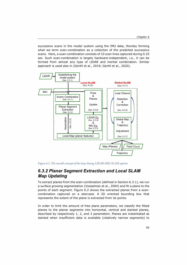
Chapter 6

95

successive scans in the model system using the IMU data, thereby forming what we term scan-combination as a collection of the predicted successive scans. Here, a scan-combination consists of 10 scan lines captured during 0.25 sec. Such scan-combination is largely hardware-independent, i.e., it can be formed from almost any type of LIDAR and inertial combination. Similar approach is used also in (Gentil et al., 2019; Gentil et al., 2020).

Figure 6.1. The overall concept of the loop-closing LIDAR-IMU SLAM system

6.3.2 Planar Segment Extraction and Local SLAM Map Updating To extract planes from the scan-combination (defined in Section 6.3.1), we run a surface growing segmentation (Vosselman et al., 2004) and fit a plane to the points of each segment. Figure 6.2 shows the extracted planes from a scan-combination captured on a staircase. A 2D oriented bounding box that represents the extent of the plane is extracted from its points. In order to limit the amount of free plane parameters, we classify the fitted planes to the planar segments into horizontal, vertical and slanted planes, described by respectively 1, 2, and 3 parameters. Planes are instantiated as slanted when insufficient data is available (relatively narrow segments) to

Simple loop closing for continuous LIDAR&IMU Planar Graph SLAM for 3D indoor environments

96

reliably classify them as horizontal or vertical. As the SLAM progresses, more scan line points are assigned to the same plane (as described below). This then may allow to better understand the plane’s orientation. If that is the case the parameterization of the plane is updated accordingly. Furthermore, to increase the robustness of the hypothesis generation, we filter out those planes that have a standard deviation of plane fitting residuals 𝜎𝜎𝑝𝑝−𝑃𝑃𝑠𝑠 higher than max_𝜎𝜎𝑝𝑝−𝑃𝑃𝑠𝑠 or a number of points 𝑁𝑁𝑝𝑝 lower than min_𝑁𝑁𝑝𝑝. Moreover, only planes that were extracted from more than one scan are included in the estimation process. This plane extraction allows for the LIDAR data to be robustly matched against the up-to-date version of the local map in SLAM. Specifically, our data association technique seeks to find correspondences between two groups of planes: (i) these planar segments (plane hypotheses) extracted recently at 𝑡𝑡𝑟𝑟 (𝑟𝑟 = n + 1, … , N ) from the scan-combination captured in 𝑁𝑁 − n = 10 time steps, i.e., 0.25 sec; and (ii) SLAM map planes (plane features) estimated in the previous time steps 𝑡𝑡𝑝𝑝, 𝑝𝑝 = 1,2, … ,𝑛𝑛.

Figure 6.2. Planar segment extraction. Left: a scan-combination consists of a few successive scans (10) captured on a staircase. Right: surface growing segmentation with the fitted planes shown as 2D bounding boxes. For visualisation purposes, the planes for ceiling and floor’s segments are not shown.

A hypothesis and a feature may represent the same planar structure; thus, they will be matched if their 2D bounding boxes overlap and if the distance and angle between them are within a certain limit. Consequently, the planar segment’s points are added to the matched plane in the Local-SLAM map; this requires an update of its 2D bounding box if the added points are outside the already seen part of that plane. The rest of the extracted planes – those that

Chapter 6

97

have not been matched with any of the previously estimated planes – are added to the SLAM map as new planes. However, closely aligned scan lines not spanning a large area do not allow for a robust estimation of a normal vector of a plane. Therefore, they are not used to generate a new plane hypothesis. The points in such scan lines are, however, still used if they can be associated to an already existing plane feature. Additionally, each point that was not part of a planar segment (i.e., is still un-associated) is associated to its closest plane feature in the map, if that point is located within the 2D bounding box of that plane and within a certain distance. After these steps, the SLAM map is updated. Some planes may have been extended and new planes may have been instantiated. As a consequence, 2D bounding boxes of nearby planes with similar normal may now overlap. Therefore, we perform a further association check between all planes in the map. The association check is similar to the plane-to-plane association step above with the only difference that here we always merge the plane with fewer points into the plane with a larger number of points as that is considered to be more reliable. This association helps to avoid multiple instantiations of the same planar structure and decreases the number of planes, which in turn reduces the complexity of the SLAM model and speeds up the mapping process.

6.3.3 State definition and Plane and Trajectory Parametrization The extracted planes are defined in the model coordinate system by the Hessian plane model:

𝑛𝑛𝑝𝑝 − 𝑑𝑑 = 0 (6.1) where 𝑛𝑛 = (𝑛𝑛𝑥𝑥 , 𝑛𝑛𝑦𝑦, 𝑛𝑛𝑧𝑧) is the plane's normal vector, 𝑝𝑝 is a point lying in the plane and 𝑑𝑑 is the signed distance to the plane (from the origin along the normal vector). Hence, plane ℎ can be expressed with angular parameters (𝜃𝜃ℎ ,𝜙𝜙ℎ,𝑑𝑑ℎ)𝑇𝑇 with an identical amount of free parameters. Note that, in our SLAM, the normal vector of a plane (𝑛𝑛) always points towards the system’s trajectory. Additionally, the area of a plane is represented by a 2D oriented bounding box (Figure 6.2), which grows as additional observations are added from the scanning, and this bounding plays an important role in the data association as described in Section 6.3.2. The platform pose parameters (x, y, z,ω,ϕ, κ) are modelled as continuous functions over time using cubic splines (Karam et al., 2019), which guarantees a level of smoothness for the final trajectory and allows for a continuous time

Simple loop closing for continuous LIDAR&IMU Planar Graph SLAM for 3D indoor environments

98

representation for individual measurements. For instance, roll ω is formulated as follows:

𝜔𝜔(𝑡𝑡) = ∑ 𝛼𝛼𝜔𝜔,𝑖𝑖 .𝐵𝐵𝑖𝑖(𝑡𝑡)𝑖𝑖 , (6.2)

where 𝛼𝛼𝜔𝜔,𝑖𝑖 is the spline coefficient for 𝜔𝜔 to be estimated on interval 𝑖𝑖 and 𝐵𝐵𝑖𝑖(𝑡𝑡) is the B-spline value at time 𝑡𝑡 on interval 𝑖𝑖.

Our SLAM is an optimization-based method that combines the LIDAR and IMU measurements together to estimate the state of the system and the SLAM map. Instead of defining state vectors for the trajectory, we define them for the observations. Adding together all LIDAR and IMU observations, the total state to be estimated 𝑑𝑑𝑡𝑡𝑡𝑡𝑡𝑡𝑠𝑠𝑠𝑠 consists of spline coefficients for each node interval 𝑖𝑖, where 𝑖𝑖 indexes the M spline intervals, and parameters of all planes, as follows:

𝑑𝑑𝑡𝑡𝑡𝑡𝑡𝑡𝑠𝑠𝑠𝑠 = [𝛼𝛼1, 𝛼𝛼2, … …𝛼𝛼𝑀𝑀, 𝑃𝑃1, 𝑃𝑃2, … … 𝑃𝑃𝐻𝐻 ] (6.3)

where 𝑗𝑗 refers to the number of LIDAR observation, 𝑗𝑗 = 1,2, … K, 𝛼𝛼𝑖𝑖 =[𝛼𝛼𝜔𝜔,𝑖𝑖 ,𝛼𝛼ϕ,𝑖𝑖 ,𝛼𝛼κ,𝑖𝑖 ,𝛼𝛼𝑥𝑥,𝑖𝑖 ,𝛼𝛼𝑦𝑦,𝑖𝑖 ,𝛼𝛼𝑧𝑧,𝑖𝑖] spline coefficients on interval 𝑖𝑖 and 𝑃𝑃ℎ = (𝜃𝜃ℎ ,𝜙𝜙ℎ,𝑑𝑑ℎ) is the parametrization of plane ℎ, ℎ = 1,2, … ,𝐻𝐻.

Here, we include the map features into the state because our purpose is to build accurate maps for mapping purposes using graph SLAM. We first formulate the LIDAR (Section 6.3.4) and IMU (Section 6.3.5) observation equations that form the equation system for Local_SLAM (Section 6.3.6) and Global_SLAM (Section 6.3.7).

6.3.4 LIDAR observation equation The LIDAR observation equation is formulated based on the expectation that the distance between a point 𝑝𝑝 and its assigned plane 𝑃𝑃ℎ = (𝑛𝑛ℎ,𝑑𝑑ℎ) equal zero (Karam et al., 2019; Vosselman, 2014). Due to the sensor noise and estimation errors, this distance is not necessarily zero, but a residual 𝑟𝑟𝑝𝑝. Consequently, for a point 𝑝𝑝j𝑚𝑚 = (𝑥𝑥𝑗𝑗𝑚𝑚,𝑦𝑦𝑗𝑗𝑚𝑚, 𝑧𝑧𝑗𝑗𝑚𝑚) in the model coordinate system (𝑚𝑚), the equation can be formulated as follows:

𝑟𝑟𝑝𝑝j𝑚𝑚 = 𝑛𝑛ℎ 𝑝𝑝j𝑚𝑚 − 𝑑𝑑ℎ, (6.4)

Chapter 6

99

The normal vector of a plane can be parametrized using the spherical coordinates (azimuth 𝜃𝜃, inclination 𝜙𝜙) and the observation equation can be rewritten as

𝑟𝑟𝑝𝑝j𝑚𝑚 = 𝑐𝑐𝑐𝑐𝑐𝑐𝜙𝜙ℎ 𝑐𝑐𝑐𝑐𝑐𝑐𝜃𝜃ℎ 𝑥𝑥𝑗𝑗𝑚𝑚 + 𝑐𝑐𝑐𝑐𝑐𝑐𝜙𝜙ℎ 𝑐𝑐𝑖𝑖𝑛𝑛𝜃𝜃ℎ 𝑦𝑦𝑗𝑗𝑚𝑚 + 𝑐𝑐𝑖𝑖𝑛𝑛𝜙𝜙ℎ 𝑧𝑧𝑗𝑗𝑚𝑚 − 𝑑𝑑ℎ, (6.5)

Accordingly, the plane 𝑃𝑃ℎ is represented as 𝑃𝑃ℎ = (𝜃𝜃ℎ , 𝜙𝜙ℎ, 𝑑𝑑ℎ , 𝑂𝑂𝐵𝐵𝐵𝐵ℎ), where 𝑂𝑂𝐵𝐵𝐵𝐵ℎ contains information about the 2D bounding box extents. The mapping system records the point 𝑝𝑝𝑗𝑗 at time 𝑡𝑡𝑗𝑗 in its platform coordinate system (𝑓𝑓), which is later transformed to the model system by:

𝑝𝑝j𝑚𝑚 = 𝑅𝑅𝑓𝑓𝑚𝑚�𝑡𝑡𝑗𝑗� 𝑝𝑝j𝑓𝑓 + 𝑣𝑣�𝑡𝑡𝑗𝑗�, (6.6)

where 𝑅𝑅𝑓𝑓𝑚𝑚�𝑡𝑡𝑗𝑗� and 𝑣𝑣�𝑡𝑡𝑗𝑗� are the time-dependent rotation matrix and translation from the platform system (𝑓𝑓) to the model system (𝑚𝑚), respectively. The continuous representation of the trajectory using splines allows the pose parameters to be derived at any time. As each recorded LIDAR point 𝑝𝑝j

𝑓𝑓 has

its own timestamp 𝑡𝑡𝑗𝑗, our SLAM transforms the point 𝑝𝑝j𝑓𝑓 to the model system

with rotation 𝑅𝑅𝑓𝑓𝑚𝑚�𝑡𝑡𝑗𝑗� and translation 𝑣𝑣�𝑡𝑡𝑗𝑗� parameters derived from the pose splines at its timestamp 𝑡𝑡𝑗𝑗 as follows:

𝑅𝑅𝑓𝑓𝑚𝑚�𝑡𝑡𝑗𝑗�

= 𝑅𝑅(�𝛼𝛼𝜔𝜔,𝑖𝑖 .𝐵𝐵𝑖𝑖�𝑡𝑡𝑗𝑗�𝑖𝑖

,� 𝛼𝛼ϕ,𝑖𝑖 .𝐵𝐵𝑖𝑖�𝑡𝑡𝑗𝑗�𝑖𝑖

,�𝛼𝛼κ,𝑖𝑖𝑖𝑖

.𝐵𝐵𝑖𝑖(𝑡𝑡𝑗𝑗)) (6.7)

𝑣𝑣�𝑡𝑡𝑗𝑗�

= (�𝛼𝛼𝑥𝑥,𝑖𝑖 .𝐵𝐵𝑖𝑖�𝑡𝑡𝑗𝑗�𝑖𝑖

,�𝛼𝛼𝑦𝑦,𝑖𝑖.𝐵𝐵𝑖𝑖�𝑡𝑡𝑗𝑗�𝑖𝑖

,�𝛼𝛼𝑧𝑧,𝑖𝑖𝑖𝑖

.𝐵𝐵𝑖𝑖(𝑡𝑡𝑗𝑗)) (6.8)

By substituting Eq. (6.6) in Eq. (6.4), we obtain the following observation equation:

𝑟𝑟𝑝𝑝j𝑚𝑚 ≝ 𝑛𝑛ℎ�𝑅𝑅𝑓𝑓𝑚𝑚�𝑡𝑡𝑗𝑗� 𝑝𝑝j𝑓𝑓 + 𝑣𝑣�𝑡𝑡𝑗𝑗�� − 𝑑𝑑ℎ, (6.9)

After linearizing Eq. (6.9) with respect to the unknown pose spline coefficients and unknown plane parameters (Vosselman, 2014) using Taylor-series expansion, the residual 𝑟𝑟𝑝𝑝j𝑚𝑚

0 for LIDAR observations is

Simple loop closing for continuous LIDAR&IMU Planar Graph SLAM for 3D indoor environments

100

𝑛𝑛ℎ0 ��𝑅𝑅𝑓𝑓𝑚𝑚0�𝑡𝑡𝑗𝑗� 𝑝𝑝j

𝑓𝑓 + 𝑣𝑣0�𝑡𝑡𝑗𝑗��� − 𝑑𝑑ℎ0

�����������������������𝑟𝑟𝑝𝑝j𝑚𝑚0

= (6.10)

−𝑛𝑛ℎ0𝜕𝜕𝑅𝑅𝑓𝑓𝑚𝑚

0�𝑡𝑡𝑗𝑗�𝜕𝜕𝜔𝜔

𝑝𝑝j𝑓𝑓� ∆𝛼𝛼𝜔𝜔,𝑖𝑖 .𝐵𝐵𝑖𝑖�𝑡𝑡𝑗𝑗�

𝑖𝑖−

𝑛𝑛ℎ0𝜕𝜕𝑅𝑅𝑓𝑓𝑚𝑚

0�𝑡𝑡𝑗𝑗�𝜕𝜕ϕ

𝑝𝑝j𝑓𝑓� ∆𝛼𝛼ϕ,𝑖𝑖 .𝐵𝐵𝑖𝑖�𝑡𝑡𝑗𝑗�

𝑖𝑖−

𝑛𝑛ℎ0𝜕𝜕𝑅𝑅𝑓𝑓𝑚𝑚

0�𝑡𝑡𝑗𝑗�𝜕𝜕κ

𝑝𝑝j𝑓𝑓� ∆𝛼𝛼κ,𝑖𝑖.𝐵𝐵𝑖𝑖�𝑡𝑡𝑗𝑗�

𝑖𝑖−

𝑛𝑛ℎ𝑥𝑥0� ∆𝛼𝛼𝑣𝑣𝑥𝑥,𝑖𝑖.𝐵𝐵𝑖𝑖�𝑡𝑡𝑗𝑗�

𝑖𝑖− 𝑛𝑛ℎ𝑦𝑦

0 � ∆𝛼𝛼𝑣𝑣𝑦𝑦,𝑖𝑖 .𝐵𝐵𝑖𝑖�𝑡𝑡𝑗𝑗�𝑖𝑖

− 𝑛𝑛ℎ𝑧𝑧0� ∆𝛼𝛼𝑣𝑣𝑧𝑧,𝑖𝑖 .𝐵𝐵𝑖𝑖�𝑡𝑡𝑗𝑗�

𝑖𝑖+

�𝑐𝑐𝑖𝑖𝑛𝑛 𝜃𝜃ℎ0𝑐𝑐𝑐𝑐𝑐𝑐𝜙𝜙ℎ0 − 𝑐𝑐𝑐𝑐𝑐𝑐𝜃𝜃ℎ0𝑐𝑐𝑐𝑐𝑐𝑐𝜙𝜙ℎ0 0� �𝑅𝑅𝑓𝑓𝑚𝑚

0�𝑡𝑡𝑗𝑗�𝑝𝑝j𝑓𝑓 + 𝑣𝑣0�𝑡𝑡𝑗𝑗�� ∆𝜃𝜃ℎ +

�𝑐𝑐𝑐𝑐𝑐𝑐 𝜃𝜃ℎ0𝑐𝑐𝑖𝑖𝑛𝑛𝜙𝜙ℎ0 𝑐𝑐𝑖𝑖𝑛𝑛𝜃𝜃ℎ0𝑐𝑐𝑖𝑖𝑛𝑛𝜙𝜙ℎ0 − 𝑐𝑐𝑐𝑐𝑐𝑐𝜙𝜙ℎ0� �𝑅𝑅𝑓𝑓𝑚𝑚0�𝑡𝑡𝑗𝑗�𝑝𝑝j

𝑓𝑓 + 𝑣𝑣0�𝑡𝑡𝑗𝑗�� ∆𝜙𝜙ℎ + ∆𝑑𝑑ℎ

where the upper index 0 denotes the approximate value, ∆𝛼𝛼𝜔𝜔,𝑖𝑖 , ∆𝛼𝛼ϕ,𝑖𝑖 , ∆𝛼𝛼κ,𝑖𝑖 , ∆𝛼𝛼𝑣𝑣𝑥𝑥,𝑖𝑖 , ∆𝛼𝛼𝑣𝑣𝑦𝑦,𝑖𝑖 ,∆𝛼𝛼𝑣𝑣𝑧𝑧,𝑖𝑖 are the unknown increments of the pose splines coefficients on interval 𝑖𝑖 and ∆𝜃𝜃ℎ ,∆𝜙𝜙ℎ,∆𝑑𝑑ℎ are the unknown increments of the parameters of plane 𝑃𝑃ℎ. Eq. (6.10) is written in general form, i.e., for arbitrarily oriented planes for which all three increments (∆θ, ∆𝜙𝜙, ∆𝑑𝑑) are estimated. However, we reduce the problem by reducing the degrees of freedom of planes, depending on the plane type. For horizontal planes, we set 𝜃𝜃 = 0, 𝜙𝜙 = 0. For vertical planes, we set 𝜙𝜙 =0. This increases the robustness of the optimization.

6.3.5 IMU observation equation The IMU in the proposed SLAM is utilized not only in the pose prediction but also in the pose estimation. From several strategies developed by Karam et al. (2020) to integrate the IMU with the LiDAR SLAM, this chapter uses the joint estimation strategy because it is the most robust of those experimented with. The equation system in this strategy consists of two types of observation equations: the LiDAR observation equation, Eq. (6.10), that is formulated for each point assigned to a plane in the SLAM map; and the IMU observation equation that is formulated for each measurement along one of the axes of the IMU sensor system (s). As the IMU measures angular velocity �̇�𝑉𝑖𝑖𝑚𝑚𝑖𝑖𝑠𝑠 =(�̇�𝜔𝑖𝑖𝑚𝑚𝑖𝑖

𝑠𝑠 , �̇�𝜑𝑖𝑖𝑚𝑚𝑖𝑖𝑠𝑠 , �̇�𝜅𝑖𝑖𝑚𝑚𝑖𝑖s ) and acceleration �̈�𝑇𝑖𝑖𝑚𝑚𝑖𝑖𝑠𝑠 = (�̈�𝑑𝑖𝑖𝑚𝑚𝑖𝑖s , �̈�𝑑𝑖𝑖𝑚𝑚𝑖𝑖s , �̈�𝑑𝑖𝑖𝑚𝑚𝑖𝑖𝑠𝑠 ) along all three

Chapter 6

101

axes over time, we formulate six IMU equations at each IMU timestamp 𝑡𝑡𝑖𝑖, Eq. (6.14) and Eq. (6.15). The IMU observation equations have been described in (Karam et al., 2020), but for completeness, they are also described here with additional details. The acceleration observation equation is formulated based on the expectation that the IMU acceleration, after the rotation to the model system and the gravity (𝑔𝑔) compensation, should correspond to the second-order derivative of the mapping system’s location �̈�𝑇𝑓𝑓𝑚𝑚 = (�̈�𝑑𝑓𝑓m, �̈�𝑑𝑓𝑓m, �̈�𝑑𝑓𝑓𝑚𝑚).

�̈�𝑇𝑓𝑓𝑚𝑚(𝑡𝑡𝑖𝑖) = 𝑅𝑅𝑓𝑓𝑚𝑚(𝑡𝑡𝑖𝑖) 𝑅𝑅𝑠𝑠𝑓𝑓 �̈�𝑇𝑖𝑖𝑚𝑚𝑖𝑖𝑠𝑠 (𝑡𝑡𝑖𝑖) − �

00𝑔𝑔� (6.11)

where 𝑅𝑅𝑠𝑠

𝑓𝑓 = 𝑅𝑅𝑧𝑧(90ᵒ) is the time-independent rotation matrix from the IMU sensor system to the frame system. However, both sides of Eq. (6.11) are not necessarily equal and the difference is termed acceleration residual 𝑟𝑟�̈�𝑇 in this chapter.

�̈�𝑇𝑓𝑓𝑚𝑚(𝑡𝑡𝑖𝑖) − 𝑅𝑅𝑓𝑓𝑚𝑚(𝑡𝑡𝑖𝑖) 𝑅𝑅𝑠𝑠𝑓𝑓 �̈�𝑇𝑖𝑖𝑚𝑚𝑖𝑖𝑠𝑠 (𝑡𝑡𝑖𝑖) + �

00𝑔𝑔� = 𝑟𝑟�̈�𝑇 (6.12)

Similarly, the following angular velocity observation equation is formulated based on the expectation that the IMU angular velocity should correspond to the first-order derivatives of the mapping system’s rotation angles �̇�𝑉𝑓𝑓𝑚𝑚 =(�̇�𝜔𝑓𝑓𝑚𝑚, �̇�𝜑f𝑚𝑚, �̇�𝜅𝑓𝑓𝑚𝑚) after the rotation to the IMU sensor system.

�̇�𝑉𝑖𝑖𝑚𝑚𝑖𝑖𝑠𝑠 (𝑡𝑡𝑖𝑖) − 𝑅𝑅𝑓𝑓𝑆𝑆(𝑡𝑡𝑖𝑖)𝑆𝑆𝑚𝑚𝑓𝑓 (𝑡𝑡𝑖𝑖)�̇�𝑉𝑓𝑓𝑚𝑚(𝑡𝑡𝑖𝑖) = 𝑟𝑟�̇�𝑉 (6.13)

where 𝑟𝑟�̇�𝑉 is the angular velocity residual at 𝑡𝑡𝑖𝑖, 𝑅𝑅𝑓𝑓𝑆𝑆= �𝑅𝑅𝑠𝑠𝑓𝑓�

𝑇𝑇and

𝑆𝑆𝑚𝑚𝑓𝑓 = �

cos𝜑𝜑 cos𝜅𝜅 sin𝜅𝜅 0− cos𝜑𝜑 sin𝜅𝜅 cos 𝜅𝜅 0

sin𝜑𝜑 0 1�𝑚𝑚

𝑓𝑓

is the transformation matrix from the model

system to the frame system; see (Karam et al., 2020) for more detail.

As the pose parameters in Eq. (6.10) are modelled using splines, the IMU measurements (acceleration and angular velocity) in the IMU equations are also modelled using splines. Although the IMU has a different (usually higher) sensing frequency than the LIDAR scanner, the use of splines enables SLAM to

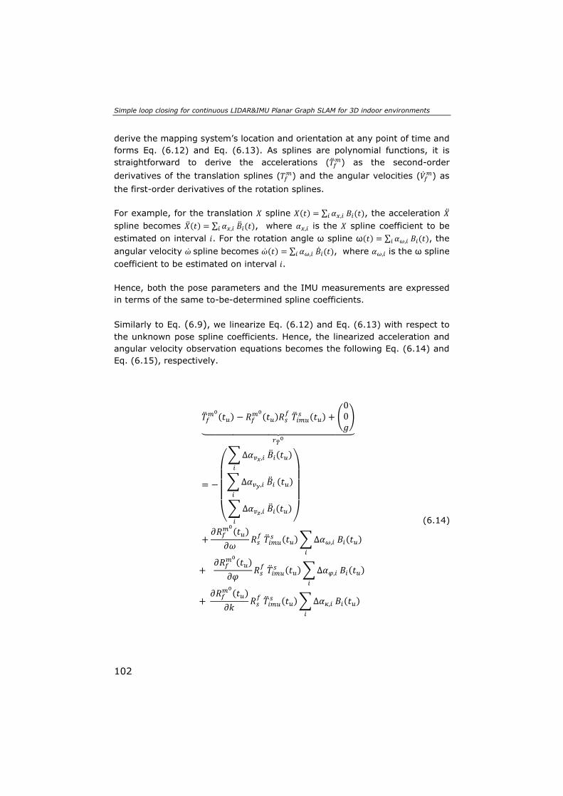
Simple loop closing for continuous LIDAR&IMU Planar Graph SLAM for 3D indoor environments

102

derive the mapping system’s location and orientation at any point of time and forms Eq. (6.12) and Eq. (6.13). As splines are polynomial functions, it is straightforward to derive the accelerations (�̈�𝑇𝑓𝑓𝑚𝑚) as the second-order derivatives of the translation splines (𝑇𝑇𝑓𝑓𝑚𝑚) and the angular velocities (�̇�𝑉𝑓𝑓𝑚𝑚) as the first-order derivatives of the rotation splines. For example, for the translation 𝑑𝑑 spline 𝑑𝑑(𝑡𝑡) = ∑ 𝛼𝛼𝑥𝑥,𝑖𝑖 𝐵𝐵𝑖𝑖(𝑡𝑡)𝑖𝑖 , the acceleration �̈�𝑑 spline becomes �̈�𝑑(𝑡𝑡) = ∑ 𝛼𝛼𝑥𝑥,𝑖𝑖 �̈�𝐵𝑖𝑖(𝑡𝑡)𝑖𝑖 , where 𝛼𝛼𝑥𝑥,𝑖𝑖 is the 𝑑𝑑 spline coefficient to be estimated on interval 𝑖𝑖. For the rotation angle ω spline ω(𝑡𝑡) = ∑ 𝛼𝛼𝜔𝜔,𝑖𝑖 𝐵𝐵𝑖𝑖(𝑡𝑡)𝑖𝑖 , the angular velocity �̇�𝜔 spline becomes �̇�𝜔(𝑡𝑡) = ∑ 𝛼𝛼𝜔𝜔,𝑖𝑖 �̇�𝐵𝑖𝑖(𝑡𝑡)𝑖𝑖 , where 𝛼𝛼𝜔𝜔,𝑖𝑖 is the ω spline coefficient to be estimated on interval 𝑖𝑖. Hence, both the pose parameters and the IMU measurements are expressed in terms of the same to-be-determined spline coefficients. Similarly to Eq. (6.9), we linearize Eq. (6.12) and Eq. (6.13) with respect to the unknown pose spline coefficients. Hence, the linearized acceleration and angular velocity observation equations becomes the following Eq. (6.14) and Eq. (6.15), respectively.

�̈�𝑇𝑓𝑓𝑚𝑚0(𝑡𝑡𝑖𝑖) − 𝑅𝑅𝑓𝑓𝑚𝑚

0(𝑡𝑡𝑖𝑖)𝑅𝑅𝑠𝑠𝑓𝑓 �̈�𝑇𝑖𝑖𝑚𝑚𝑖𝑖𝑠𝑠 (𝑡𝑡𝑖𝑖) + �

00𝑔𝑔�

�������������������������𝑟𝑟�̈�𝑇

0

= −

⎝

⎜⎜⎜⎛�Δ𝛼𝛼𝑣𝑣𝑥𝑥,𝑖𝑖 �̈�𝐵𝑖𝑖(𝑡𝑡𝑖𝑖)𝑖𝑖

�Δ𝛼𝛼𝑣𝑣𝑦𝑦,𝑖𝑖 �̈�𝐵𝑖𝑖𝑖𝑖

(𝑡𝑡𝑖𝑖)

�Δ𝛼𝛼𝑣𝑣𝑧𝑧,𝑖𝑖 �̈�𝐵𝑖𝑖(𝑡𝑡𝑖𝑖)𝑖𝑖 ⎠

⎟⎟⎟⎞

+𝜕𝜕𝑅𝑅𝑓𝑓𝑚𝑚

0(𝑡𝑡𝑖𝑖)𝜕𝜕𝜔𝜔

𝑅𝑅𝑠𝑠𝑓𝑓 �̈�𝑇𝑖𝑖𝑚𝑚𝑖𝑖𝑠𝑠 (𝑡𝑡𝑖𝑖)�Δ𝛼𝛼𝜔𝜔,𝑖𝑖 𝐵𝐵𝑖𝑖(𝑡𝑡𝑖𝑖)

𝑖𝑖

+ 𝜕𝜕𝑅𝑅𝑓𝑓𝑚𝑚

0(𝑡𝑡𝑖𝑖)𝜕𝜕𝜑𝜑

𝑅𝑅𝑠𝑠𝑓𝑓 �̈�𝑇𝑖𝑖𝑚𝑚𝑖𝑖𝑠𝑠 (𝑡𝑡𝑖𝑖)�Δ𝛼𝛼𝜑𝜑,𝑖𝑖 𝐵𝐵𝑖𝑖(𝑡𝑡𝑖𝑖)

𝑖𝑖

+ 𝜕𝜕𝑅𝑅𝑓𝑓𝑚𝑚

0(𝑡𝑡𝑖𝑖)𝜕𝜕𝜕𝜕

𝑅𝑅𝑠𝑠𝑓𝑓 �̈�𝑇𝑖𝑖𝑚𝑚𝑖𝑖𝑠𝑠 (𝑡𝑡𝑖𝑖)�Δ𝛼𝛼𝜅𝜅,𝑖𝑖 𝐵𝐵𝑖𝑖(𝑡𝑡𝑖𝑖)

𝑖𝑖

(6.14)

Chapter 6

103

�̇�𝑉𝑖𝑖𝑚𝑚𝑖𝑖𝑠𝑠 (𝑡𝑡𝑖𝑖) − 𝑅𝑅𝑓𝑓𝑠𝑠𝑆𝑆𝑚𝑚𝑓𝑓 0(𝑡𝑡𝑖𝑖)�̇�𝑉𝑓𝑓𝑚𝑚

0(𝑡𝑡𝑖𝑖)���������������������𝑟𝑟�̇�𝑉

0

= 𝑅𝑅𝑓𝑓𝑠𝑠𝑆𝑆𝑚𝑚𝑓𝑓 0(𝑡𝑡𝑖𝑖)

⎝

⎜⎜⎜⎛�Δ𝛼𝛼𝜔𝜔,𝑖𝑖 �̇�𝐵𝑖𝑖(𝑡𝑡𝑖𝑖)𝑖𝑖

�Δ𝛼𝛼𝜑𝜑,𝑖𝑖 �̇�𝐵𝑖𝑖(𝑡𝑡𝑖𝑖)𝑖𝑖

�Δ𝛼𝛼𝜅𝜅,𝑖𝑖 �̇�𝐵𝑖𝑖(𝑡𝑡𝑖𝑖)𝑖𝑖 ⎠

⎟⎟⎟⎞

+ 𝑅𝑅𝑓𝑓𝑠𝑠𝜕𝜕𝑆𝑆𝑚𝑚

𝑓𝑓 0(𝑡𝑡𝑖𝑖)𝜕𝜕𝜕𝜕

�̇�𝑉𝑓𝑓𝑚𝑚0(𝑡𝑡𝑖𝑖)�Δ𝛼𝛼𝑘𝑘,𝑖𝑖 𝐵𝐵𝑖𝑖(𝑡𝑡𝑖𝑖)

𝑖𝑖

+ 𝑅𝑅𝑓𝑓𝑠𝑠𝜕𝜕𝑆𝑆𝑚𝑚

𝑓𝑓 0(𝑡𝑡𝑖𝑖)𝜕𝜕𝜑𝜑

�̇�𝑉𝑓𝑓𝑚𝑚0(𝑡𝑡𝑖𝑖)�Δ𝛼𝛼𝜑𝜑,𝑖𝑖 𝐵𝐵𝑖𝑖

𝑖𝑖

(𝑡𝑡𝑖𝑖)

(6.15)

Eq. (6.14) and Eq. (6.15) contain only the unknown increments of the pose splines coefficients compared to Eq. (6.10), which also contains the unknown increments of the plane parameters. The IMU is pre-calibrated, see Section 6.4.5 for details.

6.3.6 Local_SLAM After each data association that associates the extracted segments in the scan-combination to the local map, Eq. (6.10) is formulated for each point assigned to a plane in the local map. As we commented above, Local-SLAM runs within a local time window that is longer than the time interval of the scan-combination. At each IMU timestamp 𝑡𝑡𝑖𝑖 within this time window, Eq. (6.14) and Eq. (6.15) are formulated. Consequently, the equation system in the Local-SLAM consists of Eq. (6.10), Eq. (6.14) and Eq. (6.15) and is solved by a least-squares solution to estimate the unknown increments 𝛥𝛥𝑑𝑑 containing increments of all pose splines coefficients and plane parameters used within the Local_SLAM time window. The cost function, Eq. (6.16), that the least squares solution seeks to minimize is the sum of squared point-to-plane (𝑟𝑟𝑝𝑝), acceleration (𝑟𝑟�̈�𝑇) and angular velocity (𝑟𝑟�̇�𝑉) residuals.

𝑎𝑎𝑟𝑟𝑔𝑔𝑚𝑚𝑖𝑖𝑛𝑛�����𝑋𝑋𝑡𝑡𝑡𝑡𝑡𝑡𝑡𝑡𝑡𝑡

���𝑟𝑟𝑝𝑝j𝑚𝑚0 �

2

𝑗𝑗

+ � �𝑟𝑟�̈�𝑇𝑗𝑗𝑖𝑖𝑚𝑚𝑖𝑖

0 �2

𝑗𝑗𝑖𝑖𝑚𝑚𝑖𝑖

+ � � 𝑟𝑟�̇�𝑉𝑗𝑗𝑖𝑖𝑚𝑚𝑖𝑖

0 �2

𝑗𝑗𝑖𝑖𝑚𝑚𝑖𝑖

�

(6.16)

Simple loop closing for continuous LIDAR&IMU Planar Graph SLAM for 3D indoor environments

104

where 𝑗𝑗 = 1,2, …𝐾𝐾 and 𝑗𝑗𝑖𝑖𝑚𝑚𝑖𝑖 = 1,2, … 𝐽𝐽𝑖𝑖𝑚𝑚𝑖𝑖 where 𝐾𝐾 and 𝐽𝐽𝑖𝑖𝑚𝑚𝑖𝑖 refer to the number of LIDAR points and the number of IMU measurements involved in Local_SLAM, respectively. Using the estimated increments 𝛥𝛥𝑑𝑑, the pose and plane parameters 𝑑𝑑 within the Local-SLAM time window are updated, see Eq. (6.17). The update process iterates and all splines are updated, to withhold the smoothness of the trajectory, until convergence.

𝑑𝑑𝑡𝑡𝑡𝑡𝑡𝑡𝑠𝑠𝑠𝑠,𝑖𝑖𝑡𝑡+1 = 𝑑𝑑𝑡𝑡𝑡𝑡𝑡𝑡𝑠𝑠𝑠𝑠,𝑖𝑖𝑡𝑡 + 𝛥𝛥𝑑𝑑 (6.17)

where 𝑖𝑖𝑡𝑡 is the number of iteration. At the end of each Local-SLAM, we generate a new scan-combination by predicting the pose parameters using the IMU data and extract the existing planes to be associated with the local map. Thus, the IMU in our SLAM is not only used to generate the graph, but it is also used to build the data association. The pose and planes parameters within the new time window are updated, using Eq. (6.17), in the local map by invoking again the Local-SLAM as addressed above.

6.3.7 Global-SLAM and Autocalibration Compared to Local_SLAM, Global-SLAM process includes also the estimation of the intrinsic sensor calibration parameters of all three scanners (auto-calibration) and the registration parameters describing the relative poses of the scanners (auto-registration). These registration and calibration parameters are updated within SLAM process (Karam et al., 2019). Consequently, the total state to be estimated 𝑑𝑑𝑡𝑡𝑡𝑡𝑡𝑡𝑠𝑠𝑠𝑠 in Global_SLAM becomes

𝑑𝑑𝑡𝑡𝑡𝑡𝑡𝑡𝑠𝑠𝑠𝑠 = [𝛼𝛼1, 𝛼𝛼2, … …𝛼𝛼𝑀𝑀, 𝑃𝑃1 𝑃𝑃2 … … 𝑃𝑃𝐻𝐻 µ 𝛹𝛹] (6.18) where µ is 8 x 1 vector containing the intrinsic sensor calibration parameters of all three scanners, except the range scale factor of one scanner, and ψ is 11 x 1 vector containing the parameters describing the relative poses of the scanners, except the vertical offset between one scanner and the other two; see (Karam et al., 2019) for more detail. After processing the whole dataset by Local-SLAM, Global-SLAM phase starts by invoking a loop closure technique that works as described in the next section. Next, one integral adjustment solves the equation system that consists of Eq. (6.10), Eq. (6.14) and Eq. (6.15) of all assigned LIDAR points and IMU

Chapter 6

105

measurements in the dataset. The least-squares optimization framework jointly optimizes the system poses and parameters of planes by minimizing the above cost function, Eq. (6.16), overall data. Similar to the Local_SLAM, the estimation process updates the total state 𝑑𝑑𝑡𝑡𝑡𝑡𝑡𝑡𝑠𝑠𝑠𝑠 iteratively (see Eq. (6.17)) until convergence. As a result, we have estimates of the calibration (µ) and registration (𝛹𝛹) parameters, the whole trajectory, i.e., all pose spline parameters, as well as all parameters of 𝑚𝑚 planes in the model coordinate system that form the Global map.

6.3.8 Loop Closure Detection and Correction The built map in our SLAM consists of planar features. Therefore, if the system has revisited a place and we have a loop closure situation, there will be two groups of planes reconstructed in this loop closure place. The first group has been reconstructed during the first visit to the place (coloured green in Figure 6.3) and the second group has been reconstructed during the second visit (coloured blue in Figure 6.3). Therefore, in the Global-SLAM phase (see Figure 6.1), the loop closure detection searches in the map for a pair of planes that meet the following criteria. First, the normal vectors of the plane-pair are pointing towards the same direction. Second, the 2D bounding boxes of the plane-pair overlap. Third, the pair of planes are separated in time, i.e., have been captured at clearly separate time instances. If such pairs of planes are detected, they are merged to modify the graph to perform loop closure correction. The graph modification is implemented through an integral adjustment process, as described in Section 6.3.7. The loop closure and update process, which represent the Global-SLAM framework, iterates until convergence, as shown in Figure 6.1. Note that merging planes is our way of modifying the SLAM graph to correct misclosure at the end of a loop. As the planar features are large (minimum area condition in Section 6.3.2) and spatially distinct, the risk of merging wrong planes is almost negligible. The plane parametrization (Section 6.3.3) and division into classes (Section 6.3.2) also further prevents the risk of merging wrong planes.

Simple loop closing for continuous LIDAR&IMU Planar Graph SLAM for 3D indoor environments

106

Figure 6.3. The loop closure schematic shows the detected planes in the loop closure area (room) from a top perspective. Left: The misclosure at the start (green)-end (blue) room. Right: After loop closure correction. For visualization purposes, the detected planes are shown without merging.

6.4 Experiments In this section, we first briefly describe the mapping system used for data collection (Section 6.4.1) and then give an overview of the sites where the datasets were collected (Section 6.4.2). Next, we present the experimental results which are divided into two parts. First, we present the results of our closing-loop SLAM system in various indoor environments (Section 6.4.3). Second, we compare the obtained point clouds to ones derived from a commercial MMS (Viametris iMS3D) and a TLS (RIEGL VZ-400) (Section 6.4.4).

6.4.1 Mobile Mapping System Figure 6.4 shows the equipment used for the data collection. It is our research multi-sensor backpack MMS (ITC-Backpack) in which the core is formed by the triple-Hokuyo LiDAR scanners (laser range finders) (Karam et al., 2019). The system configuration consists of one top scanner mounted horizontally and on a level that prevents occlusion problem by the operator, and the other two scanners are tilted and mounted to the left and right of the top scanner. Furthermore, an Xsens IMU is positioned horizontally underneath the top scanner. The selected scanners’ configuration provides a quasi-3D LiDAR point subset that consists of three scan lines at each timestamp.

6.4.2 Study Areas and Datasets We used two study areas that differ in terms of geometry, architecture and cluttering in general. The first study area is the building of ITC faculty at the University of Twente, The Netherlands. That building is a non-Manhattan world-building and has an unusually shaped design featuring slanted planes. The second study area is the Fire Brigade building in Haaksbergen, The Netherlands. That is composed of two floors and has many small rooms (dressing, laundry, showers, toilets, storage spaces) and many rooms have several doors. The building’s architecture features rounded walls and a circular bar.

Chapter 6

107

To verify the ability of the loop-closing SLAM system, experiments were carried out in seven indoor application scenarios within these two study areas. That generated seven datasets, as shown in Table 1. The data collection duration for each dataset is listed in the third column. The fourth column lists the key characteristics that were the reasons for capturing each dataset. In other words, the listed characteristics sometimes form obstacles making the captured datasets challenging and suitable to rigorously test the ability of our SLAM system. We have selected the listed scenarios in a way that the proposed SLAM can be tested in: a multi-storey space and an environment with arbitrarily oriented planes (ITC_f2f3f2_Loop and ITC_f2f5_StairCase), various staircases (ITC_f2f5_StairCase and FB_f0f1_Stairs), long and narrow corridors (ITC_f2f3f2_Loop and ITC_f1_LargeLoop) and a cluttered area with curved surfaces (FB_f1). Furthermore, the experiments’ setup aims to demonstrate the ability of the proposed SLAM in two different loop scenarios. In the first scenario, we ended the loop by revisiting the start place of our scanning (ITC_f1_SmallLoop and ITC_f1_LargeLoop), while in the second scenario, we revisited a place that is not the start or end place of our scanning (FB_f0). For the experiments, we used min_𝑁𝑁𝑝𝑝 = 100 for the minimum number of points in a planar feature, max_𝜎𝜎𝑝𝑝−𝑃𝑃𝑠𝑠 = 3 𝑐𝑐𝑚𝑚 for the maximum standard deviation of plane fitting residuals of points and 𝑂𝑂𝐵𝐵𝐵𝐵𝑝𝑝−𝑡𝑡ℎ𝑟𝑟𝑝𝑝𝑠𝑠ℎ𝑡𝑡𝑠𝑠𝑝𝑝 = 30 𝑐𝑐𝑚𝑚 for the minimum bounding box’s extent. The distance and angle thresholds for the association between the extracted planar segments and the planes in the SLAM map were 10 𝑐𝑐𝑚𝑚 and 3ᵒ, respectively. For loop closure detection, these thresholds are set to 3 m and 15ᵒ, respectively. The time interval threshold between a pair of planes depends on the loop size. For ITC_f1_SmallLoop dataset, this threshold is set to 25 𝑐𝑐𝑒𝑒𝑐𝑐, which covers an interval of 1000 scans, while for the other loops it is set to 125 𝑐𝑐𝑒𝑒𝑐𝑐, which cover an interval of 5000 scans.

Simple loop closing for continuous LIDAR&IMU Planar Graph SLAM for 3D indoor environments

108

Figure 6.4. Mobile mapping system (ITC Backpack) used for the data collection. The Velodyne scanner observations have not been used in this work. Left: scanning the central staircase in the ITC building. Right: scanning the dressing room in the Fire Brigade building.

6.4.3 Analysis of SLAM Performance As shown in Figures 6.5 and 6.6, our SLAM system could cope with both study areas and generate point clouds successfully for all datasets. A 3D animation demonstrating these point clouds is available on video1. The final column in Table 6.1 lists the number of points in each point cloud. The proposed hypothesis generation of planar structures allows the SLAM to reconstruct arbitrarily oriented planes (slanted). This was evident through the ability of SLAM to map two different staircase environments, namely the central and emergency exit staircases, in the ITC building where several slanted planes are present (Figure 6.5a&c). Figure 6.5c clearly shows the slanted planes in the exit staircase. The ability to map stairs and handle the arbitrarily oriented planar structures enables our SLAM to map multi-storey spaces in both the ITC and Fire Brigade buildings (Figure 6.5a&c and Figure 6.6b). The benefits of the proposed hypothesis generation were not limited to handling slanted planes but also extended to reconstructing the rounded walls and circular bar in the Fire Brigade datasets (Figure 6.6c). Furthermore, the cluttered first floor in the Fire Brigade building was mapped successfully.

1 https://www.youtube.com/playlist?list=PLVQwHcKd7n9O_zh_R2NDBh4-P0aVeY8bA

Chapter 6

109

The most crucial aspect in the testing of the proposed SLAM was to check the robustness in terms of loop closure detection and correction. This was evident through the ability to detect and correct the loop closure in all four different loops (Figure 6.5a,b&d and Figure 6.6a). We computed the accumulated drift at the end of each loop without any loop closure correction. The results show that our SLAM accumulates a drift of only 0.08% (0.15 𝑚𝑚) and 0.006ᵒ/𝑚𝑚 (1ᵒ) over a 183 𝑚𝑚 long acquisition trajectory on the ground floor in the Fire Brigade building. The accumulated drift is only high in the areas that have homogeneous, long corridors as is the case for the two large loops in the ITC building. However, the drift does not exceed 0.32% (0.80 𝑚𝑚) and 0.013ᵒ/𝑚𝑚 ( 2.6ᵒ) over a trajectory length of about 250 𝑚𝑚. The resulting drifts are mainly on the X and Y axes, which represent the moving direction based on the orientation of the scanned area with respect to our model system. The drift in the Z-axis direction is negligible and is smaller than the threshold used for data association, thus the system still sees the previously estimated planes for floor and ceiling in the second visit. Performing the SLAM algorithm on the first-floor loop (ITC_f1_LargeLoop) and the second-third floor loop (f2f3f2_Loop) in the ITC building was particularly challenging, mainly because of the large loop and the long narrow corridors. This is noticeable as we have the largest misclosure in these two datasets. Misclosures are predominantly caused by positioning errors in the direction of long corridors. Figure 6.7 shows the loop closure for the largest loop in our experiments (ITC_f1_LargeLoop) both with and without the proposed loop closure correction. It can be seen that, without loop closure, reobserving places introduces duplicate walls into the map.

6.4.4 Cloud to Cloud Comparison To evaluate the performance of our SLAM system, we compared the generated point clouds to those derived from a commercial MMS (Viametris iMS3D) and a TLS (RIEGL VZ-400). The point clouds have far-away points that were captured in unvisited areas through glass or open doors. As these points will often not be present in both clouds, we have discarded these points from the comparison.

Simple loop closing for continuous LIDAR&IMU Planar Graph SLAM for 3D indoor environments

110

Table 6.1. General information about captured datasets

Building Datasets

(the terminology used in the chapter)

Collection Time (m) Key characteristics

Number of

points

ITC

bui

ldin

g

ITC_f2f3f2_Loop 5

-Slanted planar structures -Narrow and long corridors -Narrow and closed staircase -Open staircase -Multi-storey space

40 x 106

ITC_f2f5_StairCase 4

-Slanted planar structures -Narrow and closed staircase -Multi-storey space

32 x 106

ITC_f1_LargeLoop 7.5 -Narrow and long corridors -Large loop

58 x 106

ITC_f1_SmallLoop 1 -Small loop 8 x 106

Fire

Bri

gade

bui

ldin

g

FB_f0 11

-There is a hall that has very large glass walls -Three large fire trucks were parked in the hall. -Small rooms

84 x 106

FB_f1 6 -Curved walls and bar -Cluttered

48 x 106

FB_f0f1_Stairs 2 -Straight stairs -Multi-storey space

15 x 106

Chapter 6

111

(a) ITC_f2f3f2_Loop

(b) ITC_f1_largeLoop

(d) ITC_f1_smalLoop

Figure 6.5. Slanted view of the generated point clouds of the ITC building datasets captured by the ITC-Backpack. Colours show plane association. The black 2D bounding boxes in (b) represent the reconstructed planes in the Global-map and the dashed red circle represents the detected loop closure area after the correction; see Figure 6.7. Parts of the last two point clouds are not shown in order to show the interior structure with the trajectory (white).

(c) ITC_f2f5f2

Simple loop closing for continuous LIDAR&IMU Planar Graph SLAM for 3D indoor environments

112

(a) FB_f0

(b) FB_f0f1_StairCase

(c) FB_f1

Figure 6.6. Top view (a & c) and slanted view (b) of the generated point clouds of the Fire Brigade building datasets captured by the ITC-Backpack. Colours show plane association. The ceiling points in (a) and (b) and parts of the point cloud in (c) are not shown in order to show the interior structure with the trajectory (white). The wavy form of the trajectory follows from a natural walking pace.

Chapter 6

113

(a) Without loop closure (b) With loop closure

Figure 6.7. The first-floor loop in the ITC building (ITC_f1_largeLoop) which is the largest loop in our experiments. (a) Top view of the walls’ points with trajectory (black) at the start (blue) and end (red) of the loop without loop closure. (b) The walls’ points and the trajectory after loop closure correction.

6.4.4.1 Comparison against a commercial mobile mapping system On the same day as our study, the first floor in the Fire Brigade building (FB_f1) was scanned by a commercial mobile mapping system, Viametris iMS3D. For comparison purposes, both our and Viametris’s point clouds were registered in the same coordinate system using rigid transformation. The registration process was performed by means of coarse registration and the ICP algorithm included in the open-source free software CloudCompare. The difference between the clouds was undetectable by eye. To quantify the deviation of our point cloud from the Viametris iMS3D cloud, we computed the cloud-to-cloud absolute distances (C2C), also using CloudCompare; see Figure 6.8. The results show that the majority of the computed distances (about 92%) are less than 3 𝑐𝑐𝑚𝑚.

Figure 6.8. ITC-Backpack and Viametris iMS3D comparison. Left: Our point cloud (red) and iMS3D cloud (green) registered in the same coordinate system. Right: Our point cloud coloured based on the distances to the iMS3D cloud

Simple loop closing for continuous LIDAR&IMU Planar Graph SLAM for 3D indoor environments

114

6.4.4.2 TLS Comparison Furthermore, we have scanned the second-third floor loop (ITC_f2f3f2_loop), as that is one of the most challenging datasets in the ITC building by RIEGL VZ-400 TLS through a series of individual scans (39 scan positions). The registration of scan positions to generate a single point cloud was performed by means of coarse registration and the ICP algorithm included in the multi-station adjustment plugin within the RiSCAN PRO software accompanying RIEGL TLS. The registration error was less than 1 𝑐𝑐𝑚𝑚. As in the previous comparison, the point clouds from our system and TLS scanner were registered in the same coordinate system. Visual inspection shows differences between the clouds. We quantified the deviation of our point cloud to the TLS cloud used as ground truth, as shown in Figure 6.9. The histogram of C2C distances shows that 86% of the computed distances are less than 20 𝑐𝑐𝑚𝑚.

Figure 6.9. ITC-Backpack and TLS comparison. Left: Our point cloud (red) and TLS cloud (green) registered in the same coordinate system. Right: Our point cloud coloured based on the C2C distances to the TLS cloud

6.4.5 Discussion and Limitations The proposed method has limitations. The detection of a standard-height vertical wall, when observed from far-away e.g., from the other end of a corridor, becomes difficult as it can be observed only within a limited tilt angle i.e., an almost horizontal scan line. In this case, the farther away the observation is made, the more uncertain it is that the observation was made from the wall and not from the floor or the ceiling. Moreover, distinguishing whether a far-away wall is vertical or slanted is also problematic. Furthermore, in some cases, the data on such a wall is thin up to a point that makes the plane extraction impossible. In such a pathological environment, e.g., a long

Chapter 6

115

homogeneous corridor, the method will start to drift (as its IMU does) along the corridor, i.e., the direction along which LiDAR observations do not serve to update the pose. To mitigate this drift and avoid degenerate motions, we slightly relaxed the association distance threshold (by a factor of two) for the linear segments that are extracted from horizontal scan lines and far away from the system in an attempt to assign the segments on the wall at the end of a corridor to the nearest plane that had been previously estimated and most probably represented this wall. Another limitation is that the state vector formulation of Eq. (6.18) assumes time-independent autocalibration of sensors. Therefore, we chose to pre-calibrate the IMU and apply fixed biases in pre-processing. The IMU is Xsens MTi-100 and, based on our results, is of high enough quality for this approach. In future work, however, we will investigate whether map accuracy could be improved if the state vector of Eq. (6.18) accounts for time-dependent calibration by introducing piece-wise calibration parameters similarly as in (Geneva et al., 2018; Gentil et al., 2020; Zhou et al., 2020). The proposed loop closure technique corrected the misclosure at the end of all loops in our datasets (Figure 6.5a,b&d and Figure 6.6a). As is commonly known, loop closure reduces errors, but also distributes errors over the whole loop to make the data internally consistent. Therefore, we compare against the TLS point cloud, where these errors clearly remain visible (Figure 6.9). For further investigation of this errors distribution, we separated out the third floor’s point cloud from the generated point cloud (ITC_f2f3f2_loop) after loop closure (Figure 6.5a). Next, we compared the segmented cloud against the corresponding TLS cloud (Figure 6.10a). The C2C distances between these two clouds demonstrate that about 89% of the computed distances are less than 20 𝑐𝑐𝑚𝑚, which is slightly higher than the percentage for the whole loop comparison (Figure 6.9). Moreover, we ran SLAM separately just on the third floor’s data. The C2C distances between the generated point cloud and the corresponding TLS cloud show that about 84% of computed distances are less than 20 𝑐𝑐𝑚𝑚, which means that the percentage of long distances (> 20 𝑐𝑐𝑚𝑚) is increased by about 5% if we do not process the whole loop and correct the misclosure. We repeated the test above on the second floor’s cloud (Figure 6.10b) and in contrast to the third floor, the percentage of long distances (> 20 𝑐𝑐𝑚𝑚) is slightly increased after the loop closure correction. This can be explained as a distribution of the larger errors on the third floor over the entire loop as a result of the loop closure.

Simple loop closing for continuous LIDAR&IMU Planar Graph SLAM for 3D indoor environments

116

(a)

(b)

Figure 6.10. Point cloud of part of the third (a) and second (b) floor in the ITC building coloured based on the distances to the corresponding TLS cloud

Introducing the scan trajectory along with the point cloud as supplementary information is advantageous for semantic interpretation (Nikoohemat et al., 2018) and space partitioning of the point cloud (Elseicy et al., 2018). Expanding this supplementary information to cover also the plane features of the SLAM map will likely be also beneficial; and part of our future work. Simultaneously, we will then address a limitation in our current work that the association of leftover points (Section 6.3.2) may lead to points being incorrectly associated onto an existing plane, before enough points are seen to instantiate a new plane.

6.5 Conclusions This article has introduced a novel loop-closing continuous-time LiDAR-IMU Graph-SLAM method to map indoor environments. The SLAM map representation is done by a set of planes. The data association technique assigns detected planar segments as new or onto existing planes, which both can have arbitrary orientations. Regardless of this, a large number of planes still remain either horizontal or vertical in built environment; a fact which we exploit to reduce the number of free parameters in the joint optimization problem, by classifying planes into horizontal, vertical, and slanted classes. Loop closure detection and correction is done by pair-wise planar feature matching, relying on the fact that the planar features are large and hence spatially distinct. Our results are compared against a commercial mapping system (iMS3D) and the ground truth (RIEGL VZ-400 TLS). Results show that our SLAM system shows comparable performance with the commercial mobile mapping system because 92% of the C2C distances, between the corresponding clouds from both systems, are less than 3 cm. While the deviation is larger to the TLS cloud, 86% of the C2C distances are less than 20 𝑐𝑐𝑚𝑚, due to the presence of long

Chapter 6

117

homogenous corridors in the compared cloud. The proposed method was verified in various scenarios, including scanning multi-storey space, staircases, large and small loops, cluttered areas, and areas surrounded by some rounded walls.

Simple loop closing for continuous LIDAR&IMU Planar Graph SLAM for 3D indoor environments

118

119

Chapter 7 - Synthesis

Synthesis

120

7.1 Scope of application

This dissertation contributes to the 3D mapping of unknown indoor environments by developing a wearable indoor mobile mapping system employing simultaneous localization and mapping (SLAM). The chapters 3 to 6 showed the progress in this development. In Chapter 3, the design of our triple-2D-LRF backpack system and the employed planar feature-based SLAM were introduced. Representing the SLAM map by planes is advantageous due to the large size and the dominant existence of planar structures in indoor environments. This chapter presented SLAM at an early stage. It only uses the LRFs configuration, i.e., LIDAR SLAM, and does not use any additional sensor for pose prediction. Instead, it relies on a simple linear extrapolation of the previously estimated trajectory to predict the pose of the next LIDAR scan for data association purposes. Consequently, the SLAM in this chapter assumes a linear change in position and rotation over a period of two LIDAR scans and can not handle a large rotation within that period. Moreover, the proposed SLAM was designed to map indoor environments with planar and vertical structures with no capability to work in more complex environments with slanted planes such as staircases. Additionally, this chapter proposed an evaluation pipeline for indoor LIDAR point clouds. The pipeline can partly evaluate the quality of the acquired point cloud of a Manhattan World building in the absence of any ground truth model. Further, this pipeline uses a floor plan (if available) as an external information source to check the quality of the generated indoor model (i.e., 3D reconstructed planes in our method) and thereby provides an overall impression of the reconstruction accuracy. The proposed evaluation pipeline is not limited to assess only the point clouds generated by the developed mapping system in this research, but provides general means. In chapter 4, the SLAM was improved by integrating an inertial measurement unit (IMU) into the LIDAR SLAM. As an alternative to the linear extrapolation used in the previous chapter, the IMU measurements were utilized to provide a more reliable prediction of the system’s position and attitude. Thus, the SLAM became capable to handle larger and more sudden rotations of the operator while scanning, which in turn leads to a more robust data association between the measured points and planes in the map. However, since the SLAM was still only based on LIDAR observations for the pose estimation, the backpack motion may be erratic in environments containing pathological geometries such as a long homogeneous corridor or a narrow room with a large glass surface in the moving direction. The LIDAR SLAM and IMU integration was deepened in Chapter 5 by including the IMU observations not only in the pose prediction, but also in the pose

Chapter 7

121

estimation to support the LIDAR SLAM in overcoming pathological pose configurations. This Chapter proposed several strategies for this integration. Based on experiments on three indoor environments in the real world, all proposed strategies led to a more robust SLAM and a better reconstruction accuracy. Chapter 6 improved SLAM further by adding three more properties that expand the scope of application of the backpack system. These added properties are the main contributions of this chapter. First, SLAM can inherently perform loop closure detection and correction. Second, SLAM exploits the IMU to predict the pose of a few successive scans which allows for the generation of a more reliable hypothesis of planar segments. This in turn allows SLAM to handle indoor environments with arbitrarily oriented planes. Third, a more reliable data association technique is based on matching planar segments with planar features in the map. The output of this chapter was a 3D LIDAR-IMU SLAM that enables the backpack system to map more complex spaces such as staircases, fancy architecture (e.g., slanted walls, non-horizontal floor) and multi-storey buildings. However, our SLAM system still faces some challenges. The main challenge is when the extracted planes do not fully constrain the pose estimate, as is the case for the homogenous narrow corridors. Although our SLAM managed to map such areas, the drift was relatively large. However, this is a common drawback of any LIDAR SLAMs.

7.2 Conclusions per objective 1) To find the optimal configuration of the LRFs of the designed

system to avoid occlusion and acquire sufficient geometrical information of the building. This objective mainly addressed the hardware problem, i.e., backpack system design, in the research. The system design has been proposed in (Vosselman, 2014) and was implemented, optimised and evaluated in this research. The system consists of three single-layer LIDAR scanners that have a limited (270°) field of view. Consequently, identifying the optimal configuration for indoor mapping purposes is more challenging compared to multi-layer 3D scanners-based systems. To do this, an experimental comparison of selected configurations was carried out. The selection of the optimal sensor configuration was built in terms of the success of the algorithm, and the accuracy and completeness of the resulting map and point cloud. This comparison utilized our evaluation techniques proposed in Chapter 3. As a result, the selected configuration consists of one top scanner mounted horizontally on a level that prevents occlusion problems by the operator, and the other two scanners are tilted and mounted to the left and right of the top scanner. In this way, the system can cover as much

Synthesis

122

as possible of the surrounding environment and ensures a good data association when passing through doors and corners.

2) To integrate the IMU with LIDAR into SLAM so that we exploit the strength of the scanning geometry for accurate positioning in 3D and the strength of the IMU in measuring short-term pose changes. The goal of this objective was to investigate the benefits that the integration of a low-cost IMU can bring to a feature-based LIDAR SLAM algorithm. The IMU measurements were utilized for pose prediction within a short time window in Chapter 4. To benefit from the IMU and avoid the drift problem, the IMU drifts are reset at the start time of each prediction window by using the position and the approximate velocity of the system estimated based on the LIDAR observations at that time. This objective was further studied in Chapter 5 in which we investigated whether the IMU observations can be used also in the pose estimation so that our SLAM can overcome pathological pose configurations and the impact of IMU’s drift remains negligible. To do so, we proposed a combination of a reliability measure for pose estimates and coordinate and known-velocity updates. This allows resetting the IMU drift without the need to a specific data capture mode as it is the case with the zero velocity updates (Chow et al., 2014). As a result, we fused the IMU and LIDAR observations together through graph optimization to estimate the state of the system and the SLAM map. Unlike recent IMU-LIDAR based graph optimizations that use a discrete pose representation (Geneva et al., 2018; Zhou et al., 2020), our graph uses splines to have a continuous-time trajectory representation.

3) To develop a hypothesis generation of arbitrarily oriented planar structures. This enables the backpack system to map some complex spaces such as staircases and fancy architecture (e.g., slanted walls, non-horizontal floor, ..etc). Unlike our system, many recently developed indoor mapping systems use multi-layer LIDAR scanners (such as Velodyne)(Blaser et al., 2019; Leica Pegasus1). At each sweep, the multi-layer scanner provides a 3D scan that is wide enough to apply a planar segmentation method and extract planes (if present). This does not apply to the single-layer LIDAR scanner that provides a single scan line at each sweep. The goal of this objective was to build a reliable hypothesis of planes that can be applied even to these single-layer scanners. To do so, the IMU was exploited to predict the pose of a few successive scans. A collection of these scans allows for the generation of a reliable hypothesis of planar structures. This enables a mapping system composed of single-layer scanners to handle indoor environments with arbitrarily oriented planes. The goal of this objective was not limited to the plane extraction but also included a three-fold

1 www.leica-geosystems.com

Chapter 7

123

classification: horizontal, vertical, and slanted planes. We reduced the degrees of freedom of planes, depending on the plane type, which in turn increased the robustness of the graph optimization for pose estimation.

4) To develop a more reliable data association that defines the

correspondences between the recently observed data by sensors and the up-to-date built map in SLAM. The most common data association method in LIDAR SLAM is the well-known scan matching with the iterative closest point (ICP) method (Besl et al., 1992). Some related works, i.e., planar SLAMs, utilize geometric elements to find the associations such as linear segment-to-plane (Vosselman, 2014) and plane-to-plane (Geneva et al., 2018; Zhou et al., 2020; Gentil et al., 2020) associations. The use of planes is advantageous due to the large size and the abundant existence of planar structures in indoor environments. Therefore, this objective utilized the resulting planar segments from the previous objective to define the correspondences between recently recorded LIDAR data and the planar features in the map. The normal vector of planes in our SLAM always points towards the system’s trajectory. This increases the robustness as nearby planes with opposite normal vector directions can not be matched. However, the closely aligned scan lines, that are not spanning a large area, do not allow for a robust estimation of planar segment parameters in the previous objective. Therefore, this objective also utilized the LIDAR points in such scan lines and points that were not part of a planar segment (i.e., remaining un-associated) by checking their association to an already existing plane feature in the map.

5) To integrate a loop closure detection and correction technique with the LIDAR-IMU SLAM system so that the system becomes able to recognize an already visited place and correct the accumulated drift by then. Many loop closure techniques use descriptors (Steder et al., 2010; Bosse & Zlot, 2013; He et al., 2016; Guo et al., 2018;) to search for correspondences between two sets of data. The goal of this objective was to use simple descriptor on spatially distinct features (planes). To reach this goal, our loop closure technique relies on planar feature-based matching. In contrast to the closest work to ours (Gentil et al., 2020) that relies on the data association check between two LIDAR scans to detect the loop, our loop closure analyses the relationship among the whole planes in the global SLAM map. This is one of the main contributions of this research. As the planar features are typically large and spatially distinct, the risk of merging wrong planes is almost negligible. The plane parametrization and division into classes in Chapter 6 also further prevents the risk of merging wrong planes and increases the robustness of our loop closure technique.

Synthesis

124

Our loop closure technique showed the ability to handle two different loop scenarios in two different indoor environments in terms of geometry, architecture and cluttering. In the first scenario, the loop was ended by revisiting the start place of the scanning, while in the second scenario, the revisited place was not the start or end place of the scanning. Experimentally, our loop closure managed to detect and correct an accumulated drift up to 80 𝑐𝑐𝑚𝑚 (i.e., 0.32%) and 2.6ᵒ (i.e., 0.013ᵒ/𝑚𝑚) over a length trajectory of about 250 𝑚𝑚. This significant drift was accumulated after scanning an indoor space that has homogenous narrow corridors.

6) To develop an evaluation pipeline for indoor laser scanning point clouds. The accuracy of indoor mobile mapping point clouds is significantly important as SLAM-based point clouds usually suffer from registration problems. Therefore, the accuracy of the captured point clouds has to be analysed and investigated. Point cloud evaluation techniques usually use ground truth data as obtained by TLS or another indoor mobile mapping system. The most common technique is a cloud to cloud comparison after transforming both clouds to the same coordinate system (Lehtola et al., 2017; Maboudi et al., 2017, 2018; Sirmacek et al., 2016; Thomson et al., 2013). Other evaluation methods use ground truth information in the form of a CAD/ building information model (BIM) (Maboudi et al., 2018; Thomson et al., 2013). Providing such ground truth data is difficult and requires a great effort. This objective used architectural constraints to do a partial evaluation in the absence of any ground truth model, or utilized the benefits of an outdated map, which is available for many buildings nowadays, in the accuracy analysis. In particular, our evaluation method utilizes the perpendicularity and parallelism characteristics predominant in indoor environments to evaluate the ability of the mapping system to capture the true geometry of its environment. In addition, the method checks the wall thickness that characterises, like parallelism, the ability of the mapping system to keep a good localisation when moving from one room to another. Although we did not consider the errors in the constructions and the outdated map, this evaluation method provided an overall impression of the reconstruction accuracy.

7.3 Reflections and outlook

In recent years a lot of efforts have been exerted in designing indoor mobile mapping systems and developing localization and mapping algorithms. However, most indoor spaces still only have 2D representations, in the shape of floor plans, compared to outdoor spaces that most have a 3D model.

Chapter 7

125

Our research is complementary to the efforts to model indoor spaces. As a result, we developed a wearable mobile system employing SLAM algorithm for indoor mapping. Our mapping system outputs the scanned environments in planar shapes, which is a popular format for the state-of-the-art methods in indoor 3D reconstruction (Nikoohemat et al., 2020). Besides 3D planes, our system generates a 3D point cloud of the scanned area and a 3D trajectory. Outputting the scan trajectory along with the point cloud as supplementary information is advantageous for semantic interpretation (Nikoohemat et al., 2018) and space partitioning of the point cloud (Elseicy et al., 2018) which are known problems in the domain of 3D indoor modelling. This means that our system provides the required data for indoor modelling (in a point cloud shape), as many other mapping systems do, and facilitates the modelling pipeline at the same time. In this regard, our SLAM pipeline can be further improved in the future to become a complete 3D indoor mapping pipeline, i.e., from scanning to modelling. Our SLAM is innovative in dealing with relatively complex indoor environments with arbitrarily oriented planes based on a single-layer scanner. The experimental results in this research show that our mapping system offers comparable performance with a commercial mobile mapping system, Viametris iMS3D, as proven by the low deviation between the point clouds generated by both systems. Consequently, mapping with our backpack with a six degrees of freedom (6DoF) SLAM achieves a similar accuracy to that of a trolley-based system with 3DoF SLAM, but with more flexibility. The IMU used in our system, based on our results, is of sufficiently high quality and needs no calibration within our SLAM pipeline. Therefore, we did not include the IMU biases in the state vector to be estimated. In future work, however, we will investigate whether a higher map accuracy can be obtained if the state vector accounts for time-dependent calibration by introducing piece-wise calibration parameters similarly as in (Geneva et al., 2018; Gentil et al., 2020; Zhou et al., 2020). Moreover, future work can investigate the integration with visual odometry to address the drawback of LIDAR SLAM in some pathological geometries. The architectural constraints-based evaluation method is limited to evaluate point clouds of Manhattan World buildings. Future work in this domain should focus on including more constraints thereby expanding the scope of application of the evaluation method. Also, consideration of errors in the constructions and the outdated map should provide a more reliable evaluation. Nowadays, more moving objects are present in indoor spaces such as robot vacuum cleaners. In addition, there are usually people moving in building interiors and it is not reasonable to evacuate a building before each scanning.

Synthesis

126

Thus, the complexity of indoor environments is not only related to geometry and architecture. The presence of moving objects and people usually decreases the overall quality of the SLAM-based map. Also, the presence of glass surfaces (e.g., walls, large windows) leads to missing or incorrect range measurements in LIDAR-based mapping systems. Therefore, it is recommended to consider including detection and tracking techniques of moving and glass objects within SLAM. In general, the system developed in this research is considered to be versatile and the versatility stems from the wide range of applications indoor mapping has nowadays such as mapping hazardous sites, indoor navigation and positioning, virtual tourism, facility management and interior design. Specifically, similar to the state-of-the-art mobile scanning systems, our system digitizes building interiors and generates point clouds quickly. Drones are considered autonomous driving vehicles that do not necessarily require a human operator. Future work should focus on building a drone with our system configuration to scan areas that are not accessible by an operator carrying a backpack such as disaster areas. Furthermore, after the success of deep learning in many applications, one can ask how can deep learning algorithms help in indoor mobile mapping? The mobile mapping system and the employed SLAM are designed to map unknown environments. Deep learning algorithms require benchmarks for training purposes. The available indoor benchmark datasets are not enough to cover all types of indoor spaces. Considering the rapid advancements in the indoor mapping domain, we expect to have sufficient training datasets soon. However, some recent works apply deep learning methods to loop closure detection (Chen et al., 2020; Memon et al., 2020). By looking at the recent advances in the indoor mapping domain, it is very soon expected to have digital maps on mobile and desktop devices for navigation in the public buildings (e.g., hospitals, shopping malls, airports) similar to Google Maps that became indispensable outdoors. The best-case scenario is to enrich the outdoor map of an area by maps of buildings existing in this area. Having such a map will enable people to effortlessly position themselves anywhere, find optimal route and reach a destination located in the interior area and not merely at the building’s entrance, thereby making the world more accessible. For example, universities usually spread out over a large campus that contains countless buildings. New employees and freshman students need a map to guide them inside and between these buildings. However, as indoor environments are denied to the global navigation satellite systems (GNSSs), indoor mobile systems can not localize themselves immediately in the global coordinate system, but in local one with respect to

Chapter 7

127

the environment. Accordingly, indoor maps are usually defined in local coordinate systems compared to outdoor maps that are defined in the global system. Thus, integrating indoor and outdoor maps requires efforts to register both maps in the same global coordinate system. To avoid such efforts, the author recommendation for future work is to focus on indoor-outdoor mobile mapping systems that make the transition between outdoors and indoors seamless and provide a more comprehensive map of the scanned area.

128

129

Bibliography Ajay Kumar, G., Patil, A. K., Patil, R., Park, S. S., & Chai, Y. H. (2017). A LiDAR

and IMU Integrated Indoor Navigation System for UAVs and Its Application in Real-Time Pipeline Classification. Sensors, 17(6), 1268. https://doi.org/10.3390/s17061268

Besl, P., McKay, N. A Method for registration of 3-D shapes. IEEE Trans. on Pattern Analalysis and Machine Intelligence (TPAMI), 14(2):239–256, 1992.

Biber, P., Andreasson, H., Duckett, T., & Schilling, A. (2004). 3D modeling of indoor environments by a mobile robot with a laser scanner and panoramic camera. Proc. of the IEEE/RSJ International Conference on Intelligent Robots and Systems (IROS), Vol. 4, 28 September – 2 October, Pp. 3430-3435.

Blaser, S., Cavegn, S., & Nebiker, S. (2018). Development of a portable high performance mobile mapping system using the robot operation system. ISPRS Annals of the Photogrammetry, Remote Sensing and Spatial Information Sciences, 4(1), 13–20. https://doi.org/10.5194/isprs-annals-IV-1-13-2018

Blaser, S., Nebiker, S., & Wisler, D. (2019). Portable image-based high performance mobile mapping system in underground environments - system configuration and performance evaluation. ISPRS Annals of the Photogrammetry, Remote Sensing and Spatial Information Sciences, 4(2/W5), 255–262. https://doi.org/10.5194/isprs-annals-IV-2-W5-255-2019

Borrmann, D.; Elseberg, J.; Lingemann, K.; Nüchter, A.; Hertzberg, J. (2008). Globally consistent 3D mapping with scan matching. Robotics and Autonomous Systems, 56(2), 130–142.

Bosse, M., & Zlot, R. (2013). Place recognition using keypoint voting in large 3D lidar datasets. Proceedings - IEEE International Conference on Robotics and Automation, 2677–2684. https://doi.org/10.1109/ICRA.2013.6630945

Bosse, M., Zlot, R., & Flick, P. (2012). Zebedee: Design of a spring-mounted 3-D range sensor with application to mobile mapping. IEEE Transactions on Robotics, 28(5), 1104–1119.

Cadena, C., Carlone, L., Carrillo, H., Latif, Y., Scaramuzza, D., Neira, J., Reid, I., & Leonard, J. J. (2016). Past, present, and future of simultaneous localization and mapping: Toward the robust-perception age. IEEE Transactions on Robotics, 32(6), 1309–1332. https://doi.org/10.1109/TRO.2016.2624754

Celik, K., Soon-Jo Chung, & Somani, A. (2008). Mono-vision corner SLAM for indoor navigation. 2008 IEEE International Conference on Electro/Information Technology, 343–348. https://doi.org/10.1109/EIT.2008.4554326

Chen, G., Kua, J., Shum, S., & Naikal, N. (2010). Indoor localization algorithms for a human-operated backpack system. 3D Data Processing Visualization and Transmission, September, 15–17.

Chen, X., Läbe, T., Milioto, A., Röhling, T., Vysotska, O., Haag, A., Behley, J., & Stachniss, C. (2020). OverlapNet: Loop Closing for LiDAR-based SLAM. Robotics: Science and Systems XVI, i.

Bibliography

130

https://doi.org/10.15607/RSS.2020.XVI.009 Choi, D. G., Bok, Y., Kim, J. S., & Kweon, I. S. (2014). Extrinsic calibration of

2D laser sensors. Proceedings - IEEE International Conference on Robotics and Automation, 3027–3033. https://doi.org/10.1109/ICRA.2014.6907295

Chow, J. C. K., Lichti, D. D., Hol, J. D., Bellusci, G., & Luinge, H. (2014). IMU and multiple RGB-D camera fusion for assisting indoor stop-and-go 3D terrestrial laser scanning. Robotics, 3(3), 247–280. https://doi.org/10.3390/robotics3030247

Cinaz, B., & Kenn, H. (2008). “Head SLAM - Simultaneous localization and mapping with head-mounted inertial and laser range sensors.” Proceedings - International Symposium on Wearable Computers, ISWC, February, 3–10.

Concha, A., Loianno, G., Kumar, V., & Civera, J. (2016). Visual-inertial direct SLAM. 2016 IEEE International Conference on Robotics and Automation (ICRA), 1331–1338. https://doi.org/10.1109/ICRA.2016.7487266

Davison, A. J., Reid, I. D., Molton, N. D., & Stasse, O. (2007). “MonoSLAM: Real-time single camera SLAM.” IEEE Transactions on Pattern Analysis and Machine Intelligence 29.6 (2007)., 29(6), 1052–1067.

De La Puente, P., & Rodriguez-Losada, D. (2015). Feature based graph SLAM with high level representation using rectangles. Robotics and Autonomous Systems, 63(P1), 80–88. https://doi.org/10.1016/j.robot.2014.09.006

Durrant-Whyte, H., & Bailey, T. (2006a). “Simultaneous localization and mapping (SLAM): part I The Essential Algorithms.” Robotics & Automation Magazine, 2, 99–110.

Durrant-Whyte, H., & Bailey, T. (2006b). “Simultaneous Localization and Mapping (SLAM): Part II.” IEEE Robotics & Automation Magazine 13.3 : 108-117.

Elseicy, A., Nikoohemat, S., Peter, M., & Elberink, S. O. (2018). Space subdivision of indoor mobile laser scanning data based on the scanner trajectory. Remote Sensing, 10(11), 1–26. https://doi.org/10.3390/rs10111815

Fernández-Moral, E., Arévalo, V., & González-Jiménez, J. (2015). Extrinsic calibration of a set of 2D laser rangefinders. Proceedings - IEEE International Conference on Robotics and Automation, 2015-June(June), 2098–2104. https://doi.org/10.1109/ICRA.2015.7139475

Filgueira, A., Arias, P., & Bueno, M. (2016). Novel inspection system , backpack-based , for 3D modelling of indoor scenes. International Conference on Indoor Positioning and Indoor Navigation (IPIN), 4-7 October 2016, Alcalá de Henares, Spain, October, 4–7.

Flint, A., Murray, D., & Reid, I. (2011). Manhattan Scene Understanding Using Monocular, Stereo, and 3D Features. 2228–2235.

García, S., López, M. E., Barea, R., Bergasa, L. M., Gómez, A., & Molinos, E. J. (2016). Indoor SLAM for Micro Aerial Vehicles Control Using Monocular Camera and Sensor Fusion. Proceedings - 2016 International Conference on Autonomous Robot Systems and Competitions, ICARSC 2016, November 2018, 205–210. https://doi.org/10.1109/ICARSC.2016.46

Geneva, P., Eckenhoff, K., Yang, Y., & Huang, G. (2018). LIPS: LiDAR-Inertial 3D Plane SLAM. IEEE International Conference on Intelligent Robots and Systems, 123–130. https://doi.org/10.1109/IROS.2018.8594463

Gentil, C. Le, Vidal-Calleja, T., & Huang, S. (2019). IN2LAMA: INertial lidar

131

localisation and mapping. Proceedings - IEEE International Conference on Robotics and Automation, 2019-May, 6388–6394. https://doi.org/10.1109/ICRA.2019.8794429

GeoSLAM Ltd. The ZEB-REVO Solution. (2020). https://geoslam.com/solutions/zeb-revo/

Grisetti, G, Stachniss, C., & Burgard, W. (2007). “Improved Techniques for Grid Mapping.” Robotics, IEEE Transactions On, 23(1), 34–46.

Grisetti, Giorgio, Kümmerle, R., Stachniss, C., & Burgard, W. (2010). A Tutorial on Graph-Based SLAM. IEEE Intelligent Transportation Systems Magazine 2.4, 31–43.

Guo, J., Borges, P. V. K., Park, C., & Gawel, A. (2018). Local Descriptor for Robust Place Recognition using LiDAR Intensity. ArXiv, 4(2), 1470–1477.

He, L., Wang, X., & Zhang, H. (2016). M2dp: A novel 3D point cloud descriptor and its application in loop closure detection. IEEE International Conference on Intelligent Robots and Systems, 2016-Novem, 231–237. https://doi.org/10.1109/IROS.2016.7759060

Henry, P., Krainin, M., Herbst, E., Ren, X., & Fox, D. (2014). RGB-D Mapping: Using Depth Cameras for Dense 3D Modeling of Indoor Environments. In Experimental Robotics, Springer Tracts in Advanced Robotics, vol. 79 (pp. 477–491). https://doi.org/10.1007/978-3-642-28572-1_33

Hussnain, Z., Elberink, S. O., & Vosselman, G. (2018). An automatic procedure for mobile laser scanning platform 6Dof trajectory adjustment. International Archives of the Photogrammetry, Remote Sensing and Spatial Information Sciences - ISPRS Archives, 42(1), 203–209. https://doi.org/10.5194/isprs-archives-XLII-1-203-2018

Hyyti, H., & Visala, A. (2015). A DCM Based Attitude Estimation Algorithm for Low-Cost MEMS IMUs. International Journal of Navigation and Observation, 2015. https://doi.org/10.1155/2015/503814

Ji, S., Qin, Z., Shan, J., & Lu, M. (2020). Panoramic SLAM from a multiple fisheye camera rig. ISPRS Journal of Photogrammetry and Remote Sensing, 159(May 2019), 169–183. https://doi.org/10.1016/j.isprsjprs.2019.11.014

Jimenez, A. R., Seco, F., Prieto, J. C., & Guevara, J. (2010). Indoor Pedestrian navigation using an INS/EKF framework for yaw drift reduction and a foot-mounted IMU. Proceedings of the 2010 7th Workshop on Positioning, Navigation and Communication, WPNC’10, 135–143. https://doi.org/10.1109/WPNC.2010.5649300

Kaijaluoto, R., Kukko, A., & Hyyppä, J. (2015). Precise Indoor Localization for Mobile Laser Scanner. International Archives of the Photogrammetry, Remote Sensing and Spatial Information Sciences - ISPRS Archives, 40(4W5), 1–6. https://doi.org/10.5194/isprsarchives-XL-4-W5-1-2015

Karam, S., Lehtola, V., & Vosselman, G. (2019). Integrating a low-cost MEMS IMU into a laser-based SLAM for indoor mobile mapping. International Archives of the Photogrammetry, Remote Sensing and Spatial Information Sciences - ISPRS Archives, 42(2/W17), 149–156. https://doi.org/10.5194/isprs-archives-XLII-2-W17-149-2019

Karam, S., Lehtola, V., & Vosselman, G. (2020). STRATEGIES TO INTEGRATE IMU AND LIDAR SLAM FOR INDOOR MAPPING. ISPRS Annals of Photogrammetry, Remote Sensing and Spatial Information Sciences, V-

Bibliography

132

1–2020(1), 223–230. https://doi.org/10.5194/isprs-annals-V-1-2020-223-2020

Karam, S., Peter, M., Hosseinyalamdary, S., & Vosselman, G. (2018). an Evaluation Pipeline for Indoor Laser Scanning Point Clouds. ISPRS Annals of Photogrammetry, Remote Sensing and Spatial Information Sciences, IV–1, 85–92. https://doi.org/10.5194/isprs-annals-IV-1-85-2018

Karam, Samer, Vosselman, G., Peter, M., Hosseinyalamdary, S., & Lehtola, V. (2019). Design, calibration, and evaluation of a backpack indoor mobile mapping system. Remote Sensing, 11(8). https://doi.org/10.3390/rs11080978

Kim, B. K. (2013). Indoor localization and point cloud generation for building interior modeling. Proceedings - IEEE International Workshop on Robot and Human Interactive Communication, 186–191.

Lagüela, S., Dorado, I., Gesto, M., Arias, P., Gonz, D., & Lorenzo, H. (2018). Behavior analysis of novel wearable indoor mapping system based on 3D-SLAM. 1–16. https://doi.org/10.3390/s18030766

Lauterbach, H. A., Borrmann, D., Heß, R., Eck, D., Schilling, K., & Nüchter, A. (2015). Evaluation of a backpack-mounted 3D mobile scanning system. Remote Sensing, 7(10), 13753–13781. https://doi.org/10.3390/rs71013753

Le Gentil, C., Vidal-Calleja, T., & Huang, S. (2020). IN2LAAMA: Inertial Lidar Localization Autocalibration and Mapping. IEEE Transactions on Robotics, 37(1), 275–290. https://doi.org/10.1109/TRO.2020.3018641

Lee, Heon-Cheol, et al. (2011). Comparison and analysis of scan matching techniques for cooperative-SLAM. Ubiquitous Robots and Ambient Intelligence (URAI), 8th International Conference on. IEEE., 165–168.

Lehtola, V. V., Kaartinen, H., Nüchter, A., Kaijaluoto, R., Kukko, A., Litkey, P., Honkavaara, E., Rosnell, T., Vaaja, M. T., Virtanen, J. P., Kurkela, M., El Issaoui, A., Zhu, L., Jaakkola, A., & Hyyppä, J. (2017a). Comparison of the selected state-of-the-art 3D indoor scanning and point cloud generation methods. Remote Sensing, 9(8), 1–26. https://doi.org/10.3390/rs9080796

Lehtola, V. V., Kaartinen, H., Nüchter, A., Kaijaluoto, R., Kukko, A., Litkey, P., Honkavaara, E., Rosnell, T., Vaaja, M. T., Virtanen, J. P., Kurkela, M., El Issaoui, A., Zhu, L., Jaakkola, A., & Hyyppä, J. (2017b). Comparison of the selected state-of-the-art 3D indoor scanning and point cloud generation methods. Remote Sensing, 9(8), 1–26. https://doi.org/10.3390/rs9080796

Lehtola, V. V., Virtanen, J.-P., Vaaja, M. T., Hyyppä, H., & Nüchter, A. (2016a). Localization of a mobile laser scanner via dimensional reduction. ISPRS Journal of Photogrammetry and Remote Sensing, 121, 48–59. https://doi.org/10.1016/J.ISPRSJPRS.2016.09.004

Lehtola, V. V., Virtanen, J. P., Vaaja, M. T., Hyyppä, H., & Nüchter, A. (2016b). Localization of a mobile laser scanner via dimensional reduction. ISPRS Journal of Photogrammetry and Remote Sensing, 121, 48–59. https://doi.org/10.1016/j.isprsjprs.2016.09.004

Leica Geosystems AG. Leica Pegasus: Backpack, Mobile Reality Capture. (2017). https://www.gefos-leica.cz/data/original/skenery/mobilni-mapovani/backpack/leica_%0Apegasusbackpack_ds.pdf

Lenac, K., Kitanov, A., Cupec, R., & Petrović, I. (2017). Fast planar surface 3D SLAM using LIDAR. Robotics and Autonomous Systems, 92, 197–220.

133

https://doi.org/10.1016/j.robot.2017.03.013 Leutenegger, S., Furgale, P., Rabaud, V., Chli, M., Konolige, K., & Siegwart, R.

(2015). Keyframe-Based Visual-Inertial SLAM Using. The International Journal of Robotics Research, 34(3), 314–334.

Lin, J., Zheng, C., Xu, W., & Zhang, F. (2021). R2LIVE: A Robust, Real-time, LiDAR-Inertial-Visual tightly-coupled state Estimator and mapping. http://arxiv.org/abs/2102.12400

Liu, T.; Carlberg, M.; Chen, G.; Chen, J.; Kua, J.; Zakhor, A. (2010). Indoor localization and visualization using a human-operated backpack system. International Conference on Indoor Positioning and Indoor Navigation (IPIN), 15-17 September 2010, Zurich, Switzerland, September, 15–17.

Maboudi, M., Bánhidi, D., & Gerke, M. (2017a). Evaluation of indoor mobile mapping systems. GFaI Workshop 3D North East 2017 (20th Application-Oriented Workshop on Measuring, Modeling, Processing and Analysis of 3D-Data), 125–134.

Maboudi, M., Bánhidi, D., & Gerke, M. (2017b). Evaluation of Indoor Mobile Mapping Systems. GFaI Workshop 3D North East 2017 (20th Application-Oriented Workshop on Measuring, Modeling, Processing and Analysis of 3D-Data), December, 125–134.

Maboudi, M., Bánhidi, D., & Gerke, M. (2018a). Investigation of geometric performance of an indoor mobile mapping system. International Archives of the Photogrammetry, Remote Sensing and Spatial Information Sciences - ISPRS Archives, 42(2), 637–642. https://doi.org/10.5194/isprs-archives-XLII-2-637-2018

Maboudi, M., Bánhidi, D., & Gerke, M. (2018b). Investigation of geometric performance of an indoor mobile mapping system. International Archives of the Photogrammetry, Remote Sensing and Spatial Information Sciences - ISPRS Archives, 42(2), 637–642. https://doi.org/10.5194/isprs-archives-XLII-2-637-2018

Makni, A., Fourati, H., & Kibangou, A. Y. (2014). Adaptive Kalman filter for MEMS-IMU based attitude estimation under external acceleration and parsimonious use of gyroscopes. 2014 European Control Conference, ECC 2014, 1379–1384. https://doi.org/10.1109/ECC.2014.6862535

Maximov, V. (2013). “Survey of Accuracy Improvement Approaches for Tightly Coupled ToA / IMU Personal Indoor Navigation System.” Proceedings of International Conference on Indoor Positioning and Indoor Navigation, October 2013, Montbeliard, France, October.

Memon, A. R., Wang, H., & Hussain, A. (2020). Loop closure detection using supervised and unsupervised deep neural networks for monocular SLAM systems. Robotics and Autonomous Systems, 126, 103470. https://doi.org/10.1016/j.robot.2020.103470

Naikal, N., Kua, J., Chen, G., & Zakhor, A. (2009). Image Augmented Laser Scan Matching for Indoor Dead Reckoning. Proc. of the IEEE/RSJ International Conference on Intelligent Robots and Systems (IROS), 4134–4141.

Nikoohemat, S., Diakité, A. A., Zlatanova, S., & Vosselman, G. (2020). Indoor 3D reconstruction from point clouds for optimal routing in complex buildings to support disaster management. Automation in Construction, 113(May 2019), 103109. https://doi.org/10.1016/j.autcon.2020.103109

Nikoohemat, S., Peter, M., Elberink, S. O., & Vosselman, G. (2018). Semantic interpretation of mobile laser scanner point clouds in Indoor Scenes using

Bibliography

134

trajectories. Remote Sensing, 10(11). https://doi.org/10.3390/rs10111754

Norris, J. (2013). “Future Trends in Geospatial Information Management: the five to ten year vision.” Ordnance Survey at the Request of the Secretariat for the United Nations Committee of Experts on Global Geospatial Information Management (UN-GGIM). Second Edition December (2015).

Otero, R., Lagüela, S., Garrido, I., & Arias, P. (2020). Mobile indoor mapping technologies: A review. Automation in Construction, 120(August). https://doi.org/10.1016/j.autcon.2020.103399

Park, C.-S., Kim, D., You, B.-J., & Oh, S.-R. (2010). Characterization of the Hokuyo UBG-04LX-F01 2D laser rangefinder. 19th International Symposium in Robot and Human Interactive Communication, 385–390. https://doi.org/10.1109/ROMAN.2010.5598672

Peter, M., Jafri, S. R. U. N., & Vosselman, G. (2017). Line segmentation of 2D laser scanner point clouds for indoor SLAM based on a range of residuals. ISPRS Annals of Photogrammetry, Remote Sensing and Spatial Information Sciences, IV-2/W4, 363–369. https://doi.org/10.5194/isprs-annals-IV-2-W4-363-2017

Raúl Feliz, Eduardo Zalama, J. G. G.-B. (2009). Pedestrian tracking using inertial sensors. JOURNAL OF PHYSICAL AGENTS, 3(1), 35. https://pdfs.semanticscholar.org/19fd/2b360a65fa0f9d26aa30c70580a0a51aafee.pdf?_ga=2.43549858.688291403.1566824400-972038305.1566824400

S. Kohlbrecher, J. Meyer, O. Von Stryk, U. K. (2011). A Flexible and Scalable SLAM System with Full 3D Motion Estimation. Int. Symp. on Safety, Security and Rescue Robotics (SSRR). http://citeseerx.ist.psu.edu/viewdoc/download?doi=10.1.1.302.2579&rep=rep1&type=pdf

Salgues, H., Macher, H., & Landes, T. (2020). EVALUATION of MOBILE MAPPING SYSTEMS for INDOOR SURVEYS. International Archives of the Photogrammetry, Remote Sensing and Spatial Information Sciences - ISPRS Archives, 44(4/W1), 119–125. https://doi.org/10.5194/isprs-archives-XLIV-4-W1-2020-119-2020

Sirmacek, B ;, Shen, Y. ;, Lindenbergh, R. ;, Zlatanova, S. ;, & Diakite, A. (2016). Comparison of ZEB1 and Leica C10 indoor laser scanning point clouds. ISPRS Annals of the Photogrammetry, Remote Sensing and Spatial Information Sciences. 143–149. https://doi.org/10.5194/isprs-annals-III-1-143-2016

Sirmacek, Beril, Shen, Y., Lindenbergh, R., Zlatanova, S., & Diakite, A. (2016). Comparison of Zeb1 and Leica C10 Indoor Laser Scanning Point Clouds. ISPRS Annals of Photogrammetry, Remote Sensing and Spatial Information Sciences, III–1, 143–149. https://doi.org/10.5194/isprsannals-iii-1-143-2016

Steder, B., Grisetti, G., & Burgard, W. (2010). Robust place recognition for 3D range data based on point features. Proceedings - IEEE International Conference on Robotics and Automation, 1400–1405. https://doi.org/10.1109/ROBOT.2010.5509401

Thomson, C., Apostolopoulos, G., Backes, D., & Boehm, J. (2013). Mobile Laser Scanning for Indoor Modelling. ISPRS Annals of Photogrammetry, Remote Sensing and Spatial Information Sciences, Vol. 2, Part. 5/W2, 11-13 November, Antalya, Turkey, 289-293.

135

Thrun, S., & Montemerlo, M. (2006). The Graph SLAM Algorithm with Applications to Large-Scale Mapping of Urban Structures. The International Journal of Robotics Research, 25(5–6), 403–429. https://doi.org/10.1177/0278364906065387

Tran, H., Khoshelham, K., & Kealy, A. (2019). Geometric comparison and quality evaluation of 3D models of indoor environments. ISPRS Journal of Photogrammetry and Remote Sensing, 149(July 2018), 29–39. https://doi.org/10.1016/j.isprsjprs.2019.01.012

Trimble. Applanix : TIMMS Indoor Mapping. Retrieved November 20, 2018, from https://www.applanix.com/products/timms-indoor-mapping.htm

Velas, M., Spanel, M., Sleziak, T., Habrovec, J., & Herout, A. (2019). Indoor and Outdoor Backpack Mapping with Calibrated Pair of Velodyne LiDARs. Sensors, 19(18), 3944. https://doi.org/10.3390/s19183944

Viametris. iMS3D - VIAMETRIS. Retrieved November 20, 2018, from http://www.viametris.com/products/ims3d/

Vosselman, G. (2014). Design of an indoor mapping system using three 2D laser scanners and 6 DOF SLAM. ISPRS Annals of the Photogrammetry, Remote Sensing and Spatial Information Sciences 2.3 (2014): 173.

Vosselman, George, Gorte, B., Sithole, G., & Rabbani, T. (2004). Recognising structure in laser scanner point clouds. International Archives of Photogrammetry, Remote Sensing and Spatial Information Sciences, 46(8), 33–38.

Wang, Z., Zhu, H., Zhou, J., & Wang, X. (2018). Loose fusion based on SLAM and IMU for indoor environment. Ninth International Conference on Graphic and Image Processing (ICGIP 2017), 1061545(April 2018), 97. https://doi.org/10.1117/12.2302929

Wen, C., Pan, S., Wang, C., & Li, J. (2016). An Indoor Backpack System for 2-D and 3-D Mapping of Building Interiors. IEEE Geoscience and Remote Sensing Letters, 13(7), 992–996.

Yang, Y., Geneva, P., Eckenhoff, K., & Huang, G. (2019). Degenerate Motion Analysis for Aided INS with Online Spatial and Temporal Sensor Calibration. IEEE Robotics and Automation Letters, 4(2), 2070–2077. https://doi.org/10.1109/LRA.2019.2893803

Yu, N., & Zhang, B. (2019). An Improved Hector SLAM Algorithm based on Information Fusion for Mobile Robot. Proceedings of 2018 5th IEEE International Conference on Cloud Computing and Intelligence Systems, CCIS 2018, 279–284. https://doi.org/10.1109/CCIS.2018.8691198

Zhang, J., & Singh, S. (2014). LOAM : Lidar Odometry and Mapping in Real - time. July. https://doi.org/10.15607/RSS.2014.X.007

Zhang, J., & Singh, S. (2017). Low-drift and real-time lidar odometry and mapping. Autonomous Robots, 41(2), 401–416. https://doi.org/10.1007/s10514-016-9548-2

Zhou, L., Koppel, D., Ju, H., Steinbruecker, F., & Kaess, M. (2020). An Efficient Planar Bundle Adjustment Algorithm. Proceedings - 2020 IEEE International Symposium on Mixed and Augmented Reality, ISMAR 2020, 136–145. https://doi.org/10.1109/ISMAR50242.2020.00035

Bibliography

136

137

Author’s Biography Samer was born in 1989 in the city of Jisr al-Shughur, Idlib, Syria where he received his primary and secondary education. In 2012, he was awarded his Bachelor’s degree (BSc) in the field of Geomatics Engineering by Aleppo University, Syria. He was top of his class and graduated with the highest distinction. As a result, he was hired to work as a teaching assistant. Next, he moved to Turkey and worked as a Geomatics Engineer at the ATILIM company. At the end of 2014, he was enrolled in the Geomatics Engineering (GEOENGINE)

Master’s program at the University of Stuttgart in Germany and awarded a DAAD scholarship. He completed his Master’s degree (MSc) in 2016. As part of his Master’s thesis, he worked at the German Aerospace Center (DLR) as a research assistant. Later, he joined the Faculty of Geo-Information Science and Earth Observation (ITC) at the University of Twente as a PhD candidate with the goal of developing a SLAM-based backpack mobile mapping system for indoor mapping. Samer’s research has resulted in the present dissertation. He has published his work at various conferences, in symposiums and in journals, all within the Remote Sensing and Photogrammetry domain. He presented and discussed his research at the following events:

Date Event Place Nov, 2017 NCG Symposium TU Delft, The Netherlands July, 2018 Indoor Mobile Mapping

Systems Workshop TU Braunschweig, Germany

Oct, 2018

ISPRS TC I Mid-term Symposium 'Innovative

Sensing'

Karlsruher Institute of Technology (KIT), Germany

Nov, 2018 NCG Symposium

Wageningen University, The Netherlands

Nov, 2019 NCG Symposium

Twente University, The Netherlands

Dec, 2019 ISPRS Workshops LowCost3D (LC3D)

INSA Strasbourg, France

Aug-Sept, 2020 XXIV ISPRS Congress Nice, France Nov, 2020 NCG Symposium TU Delft, The Netherlands

Samenvatting

138

During his PhD trajectory at ITC, he was elected by the ITC staff community to be a member of the faculty council. Besides, he delivered lectures on the Master of Geo-information Science and Earth Observation program and reviewed scientific manuscripts for relevant conferences and journals. As well as the present dissertation, Samer authored the following publications:

1) Karam, S., Peter, M., Hosseinyalamdary, S., Vosselman, G., 2018. An evaluation pipeline for indoor laser scanning point clouds. ISPRS Ann. Photogramm. Remote Sens. Spat. Inf. Sci. IV-1, 85–92.

2) Karam, S., Vosselman, G., Peter, M., Hosseinyalamdary, S., Lehtola, V., 2019. Design, calibration, and evaluation of a backpack indoor mobile mapping system. Remote Sens. 11.

3) Karam, S., Lehtola, V., Vosselman, G., 2019b. Integrating a low-cost

MEMS IMU into a laser-based SLAM for indoor mobile mapping. The International Archives of the Photogrammetry, Remote Sensing and Spatial Information Sciences: 6th International Workshop LowCost 3D – Sensors, Algorithms, Applications. editor / P. Grussenmeyer ; A. Murtiyoso ; H. Macher ; R. Assi. Vol. XLII-2/W17 Strasbourg: International Society for Photogrammetry and Remote Sensing (ISPRS). pp. 149-156.

4) Karam, S., Lehtola, V., and Vosselman, G.: Strategies to integrate imu

and lidar slam for indoor mapping, ISPRS Ann. Photogramm. Remote Sens. Spatial Inf. Sci., V-1-2020, 223–230.

5) Karam, S., Lehtola, V., and Vosselman, G. (2021). Simple loop closing

for continuous LIDAR&IMU Planar Graph SLAM for 3D indoor environments. ISPRS Journal of Photogrammetry and Remote Sensing (Accepted)

Invited talks: Karam, S., Designing and Developing a Backpack Mobile Mapping System and SLAM Algorithm for Indoor Mapping, 2020, invited to talk to the electrical engineers and computer scientists in mapping and perception team at NavVis1, the leading provider of indoor spatial intelligence solutions.

1 www.navvis.com