to beginning map projections rnimation - usgs

U. S. DEPARTMENT OF THE INTERIOR US. GEOLOGICAL SURVEY

To Beginning Rnimation Map Projections

By Go Horn*

Tau Rho Alpha* and daan Strebe' Open-File Report 91-553 A

This report is preliminary and has not been reviewed for conformitywith U.S. Geological Survey editorial standards. Any use of trade,

firm, or product names is for descriptive purposes only and does not imply endorsementby tiie U.S. Government.

Although this program has been used by the U.S. Geological Survey,no warranty, expressed or implied, is made by the USGS as to tiie accuracy and

functioning of the program and related program material, nor shall the fact of distributionconstitute any such warranty,

and no responsibility is assumed by the USGS in connection therewith.

*U.S. Geological Survey MenloPark,CA94025

i r :.._...:ivmittimHino-shi, Tokyo -to Japan 191

01

oTo stack outline j

Description

The purpose of this HyperCard guide is to describe a few of the common map projections that can be used to present, thematic data. This description of map projections enables a compiler of thematic data to select. a map projection that will portray the data effectively, and it allows the map reader to identify the map projection so that there is a mutual understanding as to how to obtain information from the thematic map. In regional mapping, the choice of a map projection is usually based on convention or availability rather than on how well the map projection portrays a particular set. of data. The best, projection for portraying thematic data about people, countries, agriculture, geology, and so on (all areal phenomena) is a map projection that preserves areal relationships..

Many map projections are derived on a developable surface (see glossary, page 4) producing a basic grid system of longitude and latitude known as the earth's graticule. From the graticule, a map projection can be defined. In this manual, four main types of map projections are described. Projections onto ( 1 ) Planes (Azimuthal), (2) Cones, (3) Cylinders, and (4) a miscellaneous category. Each of these main types has some variations, and this guide will show some of these variations. Eighteen map projections commonly used to present, thematic data are briefly described and illustrated. Also included are several examples of the map projections used by the U. S. Geological Survey for thematic maps. This guide consists of descriptive material only and does not contain a program for creating map projections.

Requirements for the diskette version of this report are: Apple Computer, Inc., HyperCard 2.0 software (not supplied) and Apple Macintosh Plus, Classic, SE. or II. The date of this Open -File Report, is

1 0/04 / 1 99 1 . OF9 1 -533-A, paper copy, 92p. OF9 1 -533 -B, 3.5-in. HD Macintosh diskette.

To select a map projection follow the arrows to Developable surfaces or click on the map projection name on this card.

This guide is organized in the following manner:

DescriptionOrganization (this card) DefinitionsGraticule (four cards) Developable surfaces

AzimuthalAspect of azimuthal map projectionsAzimuthai Equidistant (five cards)Lambert Azimuthal Equal-Area (nine cards)Orthographic (five cards)Stereographic (five cards)Gnomonic (four cards)

ConesEquidistant Conic (two cards)Albers Conic Equal-Area (seven cards)Lambert Conformal Conic (four cards)American Poly conic (three cards)Bipolar Oblique Conic Conformal (six cards)

CylindersMercator (two cards)Oblique Mercator (two cards)Transverse Mercator (five cards)Modified Transverse Mercator (three cards)

MiscellaneousGoode Homolosine (two cards)Robinson (two cards)Sinusoidal (three cards)Van der Grinten (three cards)

Selected map projections and regional thematic maps published by the U.S. Geological Survey.

References (four cards)

Page 03

To stack outline

oDEFINITION OF TERMS:

ASPECT -Individual azimuthal map projections are divided into three aspects:( 1) the polar aspect, which centers the map at one of the poles of the globe; (2) theequatorial aspect, which centers the map at the equator; and (3) the oblique aspect,which centers the map anywhere else. (The word "aspect" has replaced the word"case" in the modern cartographic literature).CONFORMALITY-A map projection is conformal when (1) meridians and parallelsintersect at right angles, and (2) at any point the scale is the same in everydirection. The shapes of very small areas and angles with very short, sides arepreserved.DEVELOPABLE SURFACE -A developable surface is a simple geometric formcapable of being flattened without stretching. Many map projections can begrouped by a particular developable surface: cylinder, cone, or plane.EQUAL AREA -A map projection is equal area when every part, as well as thewhole, has the same area as the corresponding part on the earth, at the samereduced scale.GRATICULE-The graticule is the spherical coordinate system based on lines oflatitude and longitude."INTERRUPTED"~Interruption of a projection is where the continous surfrace ofthe map is broken. All maps are interrupted, usually a map is called "interrupted"if more than one meridian is involved.LINEAR SCALE-Linear scale is the relation between a distance on a mapprojection and the corresponding distance on the earth.LINE OF TANGENCY-The line where the developable surface intersects or touchesthe globe.MAP PROJECTION -A map projection is a systematic representation of a roundbody such as the earth on a flat (plane) surface. Each map projection has specificproperties that make it useful for specific objectives.POINT OF TANGENCY-The point where the developable surface (a plane) touchesthe globe.PRIME MERIDIAN-The zero meridian (longitude 0°) which passes throughGreen wich England.SCALE FACTOR -The relation between the scale of the map projection and theactual scale of the globe.

Page 04

o oThe earth'ssphericalgraticule.

Meridians or lines of longitude

To stack outline

Prime Meridian

75 °¥90°¥

Parallels or lines of latitude

0°H.

120°V

Page 05

To select an individual property of the Earth's spherical graticule, click on that property name on this card.

Natural propertiesof the earth's spherical ^stesi© card one of two

1. Parallels are an equal distance apart.

2. Parallels are spaced equally on meridians.

3. Meridians and other great-circle arcs are straight lines, (if looked at perpendicularly to the earth's surface).

4. Meridians converge toward the poles and diverge toward the equator.

5. Meridians are equally spaced on the parallels, but their distance apart decreases from the equator to the pole.

Page 06

To select an individual property of the Earth's spherical graticule,click on that property name on this card.

Natural propertiesof the earth's spherical ©FgiSS(§B3te card two of two

6. Meridians at the equator are spaced the same as parallels.7. Meridians at 60° are half as far apart as parallels.8. Parallels and meridians cross one another at right angles.

9. The area of surface bounded by any two parallels and two meridians (a given distance apart) is the same anywhere between the same two parallels.

10. The scale factor at each point is the same in any direction.

Page 07

The earth's spherical 0 "projected"

on to a developable surface

tangency <X

ConesCylinder

+ Point of tangency

Azimuthal

Page 06

On this card

developablesurfacenameto select it.

Azimuthal

Cylinders

Miscellaneous

To stack outline

C4BhJ>

C D

In this guide map projections are grouped according to developable surfaces.

Page 09

Azimuthal(TO deuetopaDie surracesj[ TO stack outline ]

On this card click: on the map projection name to select it.

1 Azimuthal Equidistant 3 Orthographic

or2 LambertAsimuthal Equal-Area

(are mathematically derived and canotbe shown graphically)

Aspectofazimuthal map projections.

5 Gnomonic

4 Stereographic

Equatorial Aspect

Polar Aspect

\N.

7Z/

Oblique Aspect

Individual azimuthal map projections are divided into three aspects: the polar aspect, which is tangent at the pole; the equatorial aspect, which is tangent at the equator; and the oblique aspect, which is tangent any where else. The oblique aspect is generally the most useful.

Azimuthal Equidistant

iTo flzimuthai I To stack outline

Equatorial aspect

Center of mapprojection0°H.

Page


Polar aspect

O

Center of map projection9Q°N. and 120°¥.

o o Azimuthal Equidistant

Oblique aspectCenter of map projection 40° N. and 120°V.


Lines of longitude (meridians):Polar aspect; the meridians are straight lines radiating from the point of tangency.

Oblique aspect; the meridians are complex curves concave toward the point of tangency. Equatorial aspect; the meridians are complex curves concave toward a straight central meridian, except the outer meridian of a hemisphere, which is a circle.

Lines of latitude (parallels):Polar aspect; the parallels are concentric circles. Oblique aspect: the parallels are

complex curves. Equatorial aspect: the parallels are complex curves concave toward the nearest pole; the equator is straight.

Graticule spacing:Polar;

tangency

iticule spacing:Polar aspect: the meridian spacing is equal and increases away from the point oflor^nro

Linear scale:Polar aspect: linear scale is true from the point of tangency along the meridians

only. Oblique and equatorial aspects: linear scale is true from the point of tangency. In all aspects the Azimuthal Equidistant, shows distances true to scale when measured between the point of tangency and any other point on the map.

Notes:Projection is mathematically based on a plane tangent to the earth. The entire

earth can be represented. Generally the Azimuthal Equidistant map projection is used to portray less than one hemisphere; the other hemisphere can be portrayed but areas and angles are distorted. Has true direction and true distance scaling only from the point of tangency.

Uses:The Azimuthal Equidistant projection is used for radio and seismic work, because

every place in the world will be shown at its true distance and direction from the point of tangency. The U.S. Geological Survey uses the oblique aspect of the Azimuthal Equidistant in the National Atlas and for large-scale mapping of Micronesia. The polar aspect is used as the emblem of the United Nations.


c ITo Rzlmuthal I TO stack outline

Azimuthal Equidistantas used by the U, S. Geological Survey

Used in the oblique aspect in National Atlas of the United States.

Azimuthal Equidistant used as part of the symbol of the United Nations..

flzimuthalLambertAzimuthal I To stack outline]

Equal-Area Equatorial aspect

TO "as used by U.S.G.S."!

Center of map projection 0°N.an<3 120 *V.

o oPolar aspect

LambertAzimuthalEqual-Area

Center of map projection90°N.an<3 120 *¥.

o oOblique aspectCenter of map projection 40°N.an<3 120°¥.


Page 16


Lines of longitude (meridians):Polar aspect: the meridians are straight lines radiating from the point of tangency.

Oblique and equatorial aspects: meridians are complex curves concave toward a straight central meridian, except the outer meridian of a hemisphere, which is a circle.

Lines of latitude (parallels):Polar aspect: parallels are concentric circles. Oblique and equatorial aspects: the

parallels are complex curves. The equator on the equatorial aspect is a straight line.

Graticule spacing:Polar aspect: the meridian spacing is equal, on all parallels, and the parallel spacing

is unequal and decreases toward the periphery of the projection. The graticule spacing in all aspects retains the property of equivalence of area.

Linear scale:Linear scale is better than most azimuthals, but not as good as in the azimuthal

equidistant. Angular deformation increases toward the periphery of the projection. Scale increases perpendicular to the radii, that is, toward the periphery.

Notes:The Lambert Azimuthal Equal-Area projection is mathematically based on a plane

tangent to the earth. It is the only projection that can accurately represent both areas and true direction from the center of the projection. This projection generally is used to represent only one hemisphere.

US$9:

Used in numerous atlases as a equal-area map projection representing large continent-size areas to display thematic data. The polar aspect is used by the U.S. Geological Survey in the National Atlas, and for some of the Antarctica 1:250,000 Reconnaissance Series maps . The polar, oblique, and equatorial aspects are used by the Circum-Pacific Council for Energy and Mineral Resources and the U.S. Geological Survey for the Circum-Pacific Map Project.

, . , , (TO "as used by U.S.G.S."). Lambert ^ *'" v Azimuthal ^° see ^e areas covered by the

^ , , Circum-Pacific Council Map Project, Equal-Area f +K M follow the arrows or

click on the references listed below.As used by the U. S. Geological Survey and

Circum-Pacific Council for Energy and Mineral Resources for the Circum-Pacific Map Project.

American Association of Petroleum Geologists, 1977, Geographic Map of the Circum-Pacific Region, Northwest Quadrant: Tulsa, Okla., American Association of Petroleum Geologists, scale 1:10,000,000.

, 1976, Geographic Map of the Circum-Pacific Region, Antarctica Sheet: Tulsa, Okla., American Association of Petroleum Geologists, scale 1:10,000,000.

, 1976, Geographic Map of the Circum-Pacific Region, Northeast Quadrant: Tulsa, Oklahoma, American Association of Petroleum Geologists, Tulsa, Okla., scale 1:10,000,000.

, 1976, Geographic Map of the Circum-Pacific Region, Southeast Quadrant: Tulsa, Okla., American Association of Petroleum Geologists, scale 1:10,000,000.

, 1976., Geographic Map of the Circum-Pacific Region, Southwest Quadrant: Tulsa, Okla., American Association of Petroleum Geologists, scale 1:10,000,000.

, 1976, Geographic Map of the Circum-Pacific Region, Pacific Basin Sheet: Tulsa, Okla., American Association of Petroleum Geologists, scale 1:17,000,000.

, 1990, Geographic Map of the Circum-Pacific Region, Arctic Sheet: Tulsa, Okla., American Association of Petroleum Geologists, scale 1:10,000,000.

Other map projections that can be used for North America, for the World,

[TO Hlbers Conic Equal-Hrea) [TO Sinusoidal]

f To Lambert Conic ConfcrmaT) [ToGoode Homoiosinej

f To Robinson Jv '

Lambert Azimuthal Equal-Area

[Circum-Pacific Maps)

Lambert Azimuthal Equal-Area with center point 0*v 160°WV as used by the Circum-Pacific Map Project for its Pacific Basin Sheet.



Lambert Azimuthal Equal-Area with center point 70°N V 165°W., as use by the Circum- Pacific Map Project for its Arctic Sheet.

Lambert Azimuthal Equal-Area with center point 70°S V 165°W., as used by the Circum-Pacific Map Project for its Antarctica Sheet.


Lambert Azimuthal Equal-Area with center

point 35°N.,150°E., as used by Circum- Pacific Map Project for its Northwest Quadrant.


Lambert Azimuthal Equal-Area with center point 35°S, 135°E, as used by the Circum-Pacific Map Project for its Southwest Quadrant

Lambert Azimuthal Equal-Area (

[circum-Pacific Maps]

Lambert Azimuthal Equal-Area with center point J5°N V 135°W, as used by the Circum-Pacific Map Project for its Northeast Quadrant.

Lambert Azimuthal Equal-Area with center point 40°S., 100°W.,as used by the Circum- Pacific Map Project for its Southeast Quadrant.

c TO Hzimuthal )Orthographic [ To stack outline J

Equatorial aspect

Center of map projection 0°N. and 120°¥.

Orthographic

Polar aspectCenter of map projection90°H.and 120°¥.

Orthographic

O

Oblique aspectCenter of map projection 40° N. and 120 °¥.

Orthographic

Lines of longitude (meridians):Polar aspect: the meridians are straight lines radiating from the point of tangency.

Oblique aspect: the meridians are ellipses, concave toward the center of the projection. Equatorial aspect: the meridians are ellipses concave toward the straight central meridian.

Lines of latitude (parallels):Polar aspect: the parallels are concentric circles. Oblique aspect: the parallels are

ellipses concave toward the poles. Equatorial aspect: the parallels are straight and parallel.

Graticule spacing:Polar aspect: meridian spacing is equal on any parallel and increases toward the

equator, and parallel spacing decreases from the point of tangency. Oblique and equatorial aspects: the graticule spacing decreases away from the center of the projection.

Linear scale:Scale is true on the parallels in the polar aspect and on all circles centered at the pole

of the projection in all aspects. Scale decreases along lines radiating from the center of the projection.

Notes:The Orthographic projection is geometrically based on a plane tangent to the earth,

and the point of projection is at infinity. The earth appears as it would from outer space. This projection is a truly graphic representation of the earth and is a projection in which distortion becomes a visual aid. It is the most familiar of the azimuthal map projections. Directions from the center of the Orthographic map projection are true.

Uses:The U. S. Geological Survey uses the Orthographic map projection in the National

Atlas and for a World Seismicity map.

Page 26

cOrthographic

TO Hzimuthai I TO stack outline

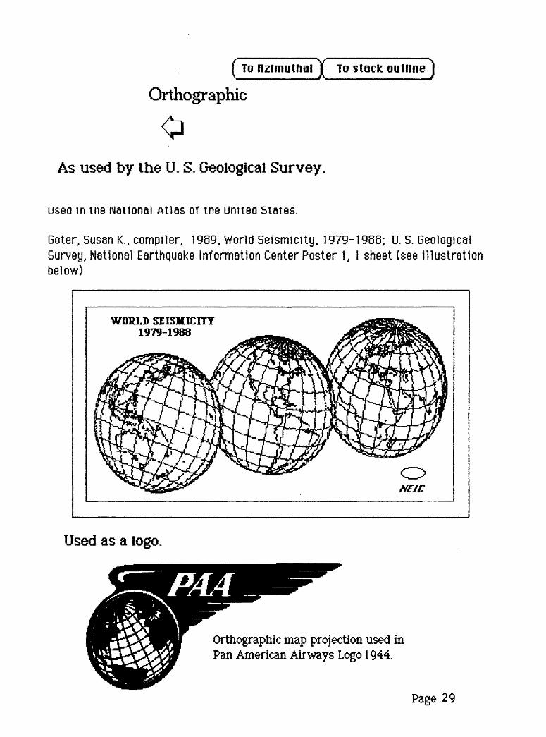
As used by the U. S. Geological Survey.

Used in the National Atlas of the United States.

Goter, Susan K., compiler, 1989, World Seismicity, 1979-1988; U. S. Geological Survey, National Earthquake information Center Poster 1, 1 sheet (see illustration below)

WORLD SEISMICITY 1979-1988

Used as a logo.

Orthographic map projection used in Pan American Airways Logo 1944.

flo flzimuthal 1

Stereographic ( TO stack outline ]

Equatorial aspect

Center of map projection Q°N.an<J 120°¥.

Stereographic

oPolar aspect

Center of map projection90 °N. and 120 °¥.

Oblique aspect

Center of map projection 40° H. and 120°¥.

Stereographic

o

Stereographic

oLines of longitude (meridians):

Polar aspect: the meridians are straight lines radiating from the point of tangency. Oblique and equatorial aspects: the meridians are arcs of circles concave toward a straight central meridian. In the equatorial aspect, the outer meridian of the hemisphere is a circle centered at the projection center.

Lines of latitude (parallels):Polar aspect: the parallels are concentric circles. Oblique aspect: the parallels are

nonconcentric arcs of circles concave toward one of the poles with one parallel being a straight line. Equatorial aspect: parallels are nonconcentric arcs of circles concave toward the poles; the equator is straight.

Graticule spacing:The graticule spacing increases away from the center of the projection in all aspects,

and it retains the property of conformality.

Linear scale:Scale increases toward the periphery of the projection. Areas are also enlarged

outward from the center.

Notes:The Stereographic projection is geometrically projected onto a plane, and the point of

the projection is on the surface of the sphere opposite the point of tangency. Circles on the earth appear as straight lines, parts of circles, or circles on the projection. Directions from the center of the Stereographic map projecton are true and lines intersect at their proper angle. Generally only one hemisphere is portrayed.

Uses:The Stereographic projection is the most widely used azimuthal projection, mainly

used for portraying large, continent-size areas of similar extent in all directions. It is used in geophysics for solving problems in spherical geometry. The polar aspect is used for topographic maps and navigational charts. The American Geographical Society uses the Stereographic map projection as the basis for its "Map of the Arctic." The U.S. Geological Survey uses the Stereographic map projection as the basis for maps of Antarctica.

c TO flzimutnai

Stereographic [ TO stack outline J

oAs used by the U. S. Geological Survey.

Used for some of the Antarctica 1:250,000 Reconnaissance series Maps.

Arctic

South America Antarctica

Africa "

Gnomonic

Equatorial aspect

f To Rzimuthal J

f To stack outline J

Gnomonic

o oPolar aspect

Page

Gnomonic

Oblique aspect

f TO Hzimutnai T TO stack outline 1

Gnomonic

oLines of longitude (meridians):

Polar aspect: the meridians are straight lines radiating from the point of tangency. Oblique and equatorial aspects: the meridians are straight lines.

Lines of latitude (parallels):Polar aspect: the parallels are concentric circles. Oblique and equatorial aspects:

parallels are ellipses, parabolas, or hyperbolas concave toward the poles (except for the equator, which is straight).

Graticule spacing:Polar aspect: the meridian spacing is equal and increases away from the pole. The

parallel spacing increases very rapidly from the pole. Oblique and equatorial aspects: the graticule spacing increases very rapidly away from the center of the projection.

Linear scale:Linear scale and angular and areal deformation are extreme, rapidly increasing

away from the center of the projection.

Notes and uses:The Gnomonic projection is geometrically projected onto a plane, and the point of

projection is at the center of the earth. It is impossible to show a full hemisphere with one Gnomonic map. It is the only projection in which any straight line is a great circle, and it is the only projection that shows the shortest distance between any two points as a straight line. Consequently, it is used in seismic work because seismic waves travel approximately in great circles. The Gnomonic projection is used together with the Mercator projection for navigation.

Page 36

fro deuelopable surfacesjf To stack outline

Cones

1 Equidistant Conic

On this card click on the

map projection nameto select it.

2 Albers Conic Equal-Area

3 Lambert Conformal Conic

4 American Polyconic

5 Bipolar Oblique Conic Conformal

There are five conic map projections

in this guide,

Equidistant Conic (or Simple Conic)

f To Cones 1

rvstack outline

Standard Parallels 20°N,60°N.

oTo cones

Equidistant Conic (or Simple Conic)

I TO stack outline

Lines of longitude (meridians):Meridians are straight lines converging on a polar axis. When one of the standard

parallels is at the pole (90° N. or S.) then the meridians converage at the pole.

Lines of latitude (parallels):Parallels are arcs of concentric circles, concave toward a pole.

Graticule spacing:Meridian spacing is true on the standard parallels and decreases toward the pole.

Parallels are spaced at true scale along the meridians. Meridians and parallels intersect each other at right angles. The graticule is symmetrical.

Linear scale:Linear scale is true along all meridians and along the standard parallel or parallels.

Notes:Projection is mathematically based on a cone that is tangent at one parallel or

conceptually secant at two parallels. North or South Pole is represented by an arc.

Uses:The Equidistant Conic projection is used in atlases for portraying

mid-latitude areas. It is good for representing regions with a few degrees of latitude lying on one side of the Equator. The Kavraisky's fourth map projection is an Equidistant conic map projection in which standard parallels are chosen to minimize overall error.

[ To Cones

Albers Conic Equal-Area , , aM , ,-)

f To "as used bg U.S.G.S." ]

Standard Parallels

Compairwith Lambert Conformal Conic using the same standard parallels.

Albers Conic Equal-Area

Lines of longitude (meridians):Meridians are straight lines converging on the polar axis., but not at the pole.

Lines or latitude (parallels):Parallels are arcs of concentric circles concave toward a pole.

Graticule spacing:Meridian spacing is equal on the standard parallels and decreases toward the poles.

Parallel spacing decreases away from the standard parallels and increases between them. Meridians and parallels intersect each other at right angles. The graticule spacing preserves the property of equivalence of area. The graticule is symmetrical.

Linear scale:Linear scale is true on the standard parallels. Maximum scale error is 1.25 percent

on a map of the contignous United States (46 states) with standard parallels of 29.5° N. and 45-5° N.

Notes:Projection is mathematically based on a cone that is conceptually secant on two

parallels. No areal deformation. North or South Pole is represented by an arc. Retains properties at various scales; indivdual sheets can be joined along their edges. Dr. Albers derived this projection and published about it in 1605.

Uses:Used for thematic maps requiring correct areas. Used for large countries with an

east-west orientation. Maps for Alaska based on the Albers Equal-Area Conic use standard parallels 55° N. and 65° N.; for Hawaii, the standard parallels are 6° N. and 16° N . The National Atlas of the United States, United'States Base Map (46 states), and the Geologic map of the United States all are based on standard parallels of 29-5° N. and 45-5° N.

[ To Cones J To stack outline

Albers Conic Equal-Area

o oAs used by the U.S. Geological Survey.

1932 Geologic map of the United States 1:2,500,000

1933 Base map, United States 1 :5,000,000

1962 Tectonic map of the United States 112,500,000

1965 Base map, United States 1:3,165,000

1970 National Atlas of United States 1:2,000,000 and 1:7,500,000

1961 Base map of United States 1:2,500,000

1967 Base map of United States 1 -.2,500,000

1972 Base map of United States 1:2,500,000

1974 Geologic map of the United States 1:2,500,000

1950 Geologic map of Alaska 1:2,500,000

1953 Generalized structural, lithologic, andphysiographic provinces on the fold andthrust belts of the United States 1: 2,500,000

Other map projections that can be used for North America

(TO Lambert Conic Con formal] [To Orthographic]

(TO Lambert Rzimuthal Equal-firea] MO Sinusoidal 1

oAlbers Conic Equal-Area50-State map of the United States

Standard Parallels

Outline represents area covered by the U. S. Geological Survey's Geologic and Tectonic Maps based on the base map entitled

"United States" at the scale of 1:2,500,000, two sheets, using standard parallels 29-5°N. and 45-5°N.

Albers Conic Equal-Area46 - State map of the United States

Standard Parallels 2 9.5*11,45.5°N.

Outline represents: area covered by the U. S. Geological Survey's Geologic and Tectonic Maps based on the base map entitled

"United States" at the scale of 1:2,500,000, .two sheets, using standard parallels 29-5°N. and 455°N.

oAlbers Conic Equal-Area46- State map of the United States

Standard Parallels

Outline represents area covered by thematic maps in The National Atlas of the United States of America at

the scale of 1:7,500,000 using standard parallels 295°N and

To stack outline

Albers Conic Equal-Area Alaska

Standard Parallels

Outline represents area covered by the I960 Geologic Map of Alaska

U. S. Geological Survey Scale 1: 2, 5000, 000 using Standard Parallels 55°N. and 65°N.

(two sheets)

Page 45

LambertConformalConic

[ To Cones jc To stack outline

f To "asuseddgU.S.G.S." 1

Standard Parallels

Compair with Albers Equal-Area using the same standard parallels.

o LambertConformalConic

Lines of longitude (meridians):Meridians are straight lines converging at a pole.

Lines of latitude (parallels):Parallels are arcs of concentric circles concave toward a pole and centered at the pole.

Graticule spacing:Meridian spacing is true on the standard parallels and decreases toward the pole.

Parallel spacing inceases away from the standard parallels and decreases between them. Meridians and parallels intersect each other at right angles. The graticule spacing retains the property of conformant?. The graticule is symmetrical.

Linear scale:Linear scale is true on standard parallels. Maximum scale error is 2.5 percent on a

map of the contignous United States (46 states) with standard parallels at 33° N. and 45° N.

Notes:Projection is mathematically based on a cone that is tangent at one parallel or (more

often) that is conceptually secant on two parallels. Areal distortion is minimal but increases away from the standard parallels. North or South Pole is represented by a point: the other pole cannot be shown. Great circle lines are approximately straight. Retains its properties at various scales: sheets can be joined along their edges. The projection was described 1772 by Johann Heinirich Lambert

Uses:Used for large countries in the mid -latitudes having an east- west orientation. The

United States (50 states) Base Map uses standard parallels at 37° N. and 65° N. Some of the National Topographic Map Series 7.5-minute and 15-minute quadrangles and the State Base Map Series are constructed on the Lambert Conformal Conic map projection. The latter series uses standard parallels of 33° N. and 45° N. Aeronautical charts for Alaska use standard parallels at 55° N. and 65° N. The National Atlas of Canada uses standard parallels at 49° N. and 77° N. On the previous card, the outline represents the United States (50 states) Base Map.

To Cones

\PI To stack outline

LambertConformalConic

As used by the U.S. Geological Survey.

Used for some of tlie State Base Map Series and for some of the 7.5-mirmte and 15-minute quadrangles of the National Topographic Map Series.

1965 East Coast bathymetric maps

1975 Base map, The United States

1:1,000,000

1:6,000,000 and 1:10,000,000

Other map projections that are used for the 7.5-minute and 15-minute quadrangles of the National Topographic Map Series.

To Transuerse Mercator[ To flmerican Poly conic J

Other map projections that can be used for North America,

(TO fllbers Conic Equal-flrea J

I To Lambert Rzimuthal Equal-flrea I

[To Sinusoidal J

LambertConforxnalConicStandard Parallels 33°N. and 45°N.

Lambert p » *uoniorma iConic

Outline represents area covered by " S * Geolo§ical Survey's base map entitled

The United States" at the scalesof l :^ooaooo ancj l . 1 0^00o,ooo,

using Standard Parallels 3?°N. and 65°N.

Standard Parallels

( To Cones ][ To stack outline]

American Polyconic

American Polyconic

Lines of longitude (meridians):Meridians are complex curves, concave toward a straight central meridian.

Lines of latitude (parallels):Parallels are nonconcentric circles except for a straight equator.

Graticule spacing:Meridian spacing is equal and decreases toward the poles. Parallels are spaced true

to scale on the central meridian, and the spacing increases toward the east and west borders. The graticule spacing results in a compromise of all properties.

Linear scale:Linear scale is true along each parallel and along the central meridian. Maximum scale

error is 7 percent on a map of the United States (45 states).

Notes:Projection is mathematically based on a infinite number of cones tangent to an infinite

number of parallels. Distortion increases away from the central meridian. Has both areal and angular deformation, but these are small for a small area. This projection was specifically devised for early maps of the United States.

Uses:Used for areas with a north-south orientation. Only portrays true shape, area,

distance, and direction along the central meridian. Formerly used as the base of the 7.5- and 15-minute quadrangles of the National Topographic Map Series. Individual sheets of this series can be edge-joined since they are drawn with straight meridians. They cannot be mosaicked beyond a few sheets.

Page

[ TO cones ][TO cones TO stack outline

American Polyconic

as used by the U. S, Geological Survey

Used for some of the 7.5-minute and 15-minute quadrangles of the National Topographic Map Series.

Other map projections that are used for the 7,5-minute and 15-minute quadrangles of the National Topographic Map Series.

( To Lambert Conic Confermal j

( To Transuerse Mercator 1

Bipolar Oblique Conic Conformal

To Cones J

f To stack outline J

( To "as used by U.S.G.S." )

Outline represents area covered by the Bipolar Oblique Conic Conformal developed by Osborn M. Miller and William A. Briesemeister of the American Geographical Society in 1941.

from: An Album of Map Projections, U.S.G.S. PP. M53,P- 99

Page


Lines of longitude (meridians):Meridians are complex curves, concave toward the center of the projection.

Lines of latitude (parallels):Parallels are complex curves concave toward the nearst pole.

Graticule spacing:Graticule spacing increases away from the lines of true scale and retains the property

of conformality.

Linear scale:Linear scale is true along two lines that do not lie along any meridian or parallel.

Scale is compressed between these lines and expanded beyond them. Linear scale is generally good, but there is as much as a 10 percent error at the edge of the projection. Areas are also compressed or expanded.

Notes:Projection is mathematically based on two cones whose apexes are 104° apart, and

which conceptually are obliquely secant to the sphere along lines (lines of tangency) following the trend of North and South America. See next card for illustration of "lines of tangency".

Uses:Used to represent one or both of the American continents. Examples are the

Basement map of North America and the Tectonic map of North America. See outlines of these maps, on next cards.

Page 5?

Tectonic map


Basement map

Lines of tangency

Page 56

[ To Cones j[ To stack outline

1965

1967

1965

1969

1976

1951


as used by the U. S. Geological Survey

Geologic map of the United States

Basement map of North America

1:5,000,000

1:5,000,000

Basement rock map of the United States 1: 2,500,000

Tectonic map of North America

Sub-surface Temperature map of North America

Metallogenic map of North America

1:5,000,000

1:5,000,000

1:5,000,000

Other map projections that can be used for North America.

Lambert Conic Conformal[To fllbers Conic Equal-fireaj

f To Lambert flzimuthal Equal-flrea J (TO Sinusoidal)

Outline represents,Tectonic Map of North America


Outline represents area covered by Basement Map of North America 1:5,000,000.

( To stack outline J


Outline represents area covered by Tectonic Map of North America (1969)and Metallogenic Map of North America (1961), both at the scale of 1:5,000,000.

MO deuelopable surfaces]! To stack outline J

Cylindrical

1 Mercator

On this card click on the map projection name

to select it.

2 Oblique Mercator

3 Transverse Mercator

There are four cylindrical

map projections in this guide,

4 Modified Transverse Mercator

Mercator[TO cylindrical^ To stack outline

[TO Cylindrical J To static outline ]

Mercator yap projections

o that should be used for the world.

Lines of longitude (meridians): fl ~.. .^i., ... . . . . . , To Sinusoidal IMeridians are straight and parallel. I J

.. .. ... . t < x To Goode Homolosine)Lines of latitude (parallels): V,____________JLatitude lines are straight and parallel. f TO R b'n }

Graticule spacing:Meridian spacing is equal, and the parallel spacing increases away from the equator.

The graticule spacing retains the property of conformaiity. The graticule is symmetrical. Meridians and parallels intersect at right angles.

Linear scale:Linear scale is true along the equator only (line of tangencyX or along two parallels

equidistant from the equator (the secant form). Scale can be determined by measuring one degree of latitude, which equals 60 nautical miles, 69 statute miles, or 111 kilometers.

Notes:Projection can be thought of as being mathematically based on a cylinder tangent at

the equator. Any straight line is a constant- azimuth (rhumb) line. Areal enlargement is extreme away from the equator; poles cannot be represented. Shape is true only within any small area. Reasonably accurate projection within a 15° band along the line of tangency.

Uses:An excellent projection for equatorial regions. Otherwise the Mercator is a special-

purpose map best suited for navigation. Secant constructions are used for large-scale coastal charts. The use of the Mercator map projection as the base for nautical charts is universal. Examples are the charts published by the National Ocean Survey., U. S. Dept. of Commerce. It should not be used for world maps or for maps of North America.

Map projections [ To fllbers Conic Equal-flrea Jthat should beused for the world. ________________

PflCf£ 64

. (To Lambert Rzimuthal

(To Sinusoidal J

f auiuno xoeis 01 TieoupunfiD oil

[TO cylindrical J To stack outline

Oblique Mercator

Lines of longitude (meridians):Meridians are complex curves concave toward the line of tangency, except each 150th

meridian is straight.

Lines of latitude (parallels):Parallels are complex curves concave toward the nearest pole.

Graticule spacing:Graticule spacing increases away from the line of tangency and retains the property of

conformality.

Linear scale:Linear scale is true along the line of tangency, or along two lines equidistant from and

parallel to the line of tangency.

Notes:Projection is mathematically based on a cylinder tangent along any great circle other

than the equator or a meridian. Shape is true only within any small area. Areal enlargement increases away from the line of tangency. Reasonably accurate projection v/ithin a 15° band along the line of tangency.

Uses:Useful for plotting linear configurations that are situated along a line oblique to the

earth's equator. Examples are: NOAA plane coordinates in the Aleutoin Islands ,NASA Surveyor Satellite tracking charts, ERTS flight indexes, strip charts for navigation, and the National Geographic Society's maps "West Indies,""Countries of the Caribbean,""Hawaii,"and "New Zealand."

[ To Cylindrical

Transverse Mercator [ TO stack outline j

f To "asusedbyU.S.G.S." 1

t/ Transverse Mercator

(_ Transverse Mercator

Page 66

Transverse Mercator

Lines of longitude (meridians):Meridians are complex curves concave toward a straight central meridian that is

tangent to the globe. The straight central meridian intersects the equator and one meridian at a 90° angle.

Lines of latitude (parallels):Parallels are complex curves concave toward the nearest pole; the equator is straight.

Graticule spacing:Parallels are spaced at their true distances on the straight central meridian. Graticule

spacing increases away from the tangent meridian. The graticule retains the property of conformality.

Linear scale:Linear scale is true along the line of tangency, or along two lines equidistant from

and parallel to the line of tangency.

Notes:Projection is mathematically based on a cylinder tangent to a meridian. Shape is

true only within any small area. Areal enlargement increases away from the tangent meridian. Reasonably accurate projection within a 15° band along line of tangency. Cannot be edge-joined in an east-west direction as each sheet has its own central meridian. First described by J. H. Lambert in 1772.

Uses:Used where the north-south dimension is greater than the east-west dimension.

Used as the base for the U.S.Geological Survey's l:250,OQQ-scale series and for some of the 7.S-minute and 15-minute quadrangles of the National Topographic Map Series.

[TO cylindrical J To stack outline )

Transverse Mercator

Transverse Mercatoras used by the U, S, Geological Survey

Used for all of the l:250,000-scale and for some of the 7.5-rninute and 15-minute quadrangles of the National Topographic Map Series.

1962 Base Map, North America 1:5,000,000 and 1:10,000,000

1966, Coal Map of North America 1: 5,000,000

Other map projections that are used for the 7,5-minute and 15-minute quadrangles of the National Topographic Map Series,

I To Lambert Conic Conformal J I TO Rmerican Poiyconic j

Other map projections that can be used for North America.

[ To fllbers Conic Equal-Rrea J [To Sinusoidal J

[ To Lambert Rzimuthai Equal-firea j [ To Lambert Conic Conformal J

Transverse MercatorOutline represents area covered by U. S. Geological Survey's

base map entitled "North America" at 1:5,000,000 and 1:10,000,000

Central Meridian 100°West

To stack outline(TO cylindrical) K f

f To "as used bg U.S.G.S." J

Modified Transverse Mercator

Pre-1973 Editions Curved Meridians

Post-1973 Editions Straight Meridians

Modified Transverse Mercator

Lines of longitude (meridians):On pre-1973 editions of the Alaska Map E, meridians are curved concave toward the

center or the projection. On post-1973 editions the meridians are straiglit

Lines of latitude (parallels): Parallels are arcs concave to the pole.

Graticule spacing:Meridian spacing is approximately equal and decreases toward the pole. Parallels

are approximately equally spaced. The graticule is symmetrical on post-1973 editions of the Alaska Map E.

Linear scale:Linear scale is more nearly correct along the meridians than along the parallels.

Notes:The Alaska Map E was adapted from a set of Transverse Mercator projections 6°

wide and approximately 16° long, repeated east and west of an arbitrary point of origin until a projection 72° wide was obtained. The post-1973 editions of the Alaska Map E more nearly approximate an equidistant conic map projection.

Uses:The U.S.Geological Survey's Alaska Map E at the scale of 1:2,500,000. The previous

card represents the 195^ edition. The 1973 edition is similar, but the meridians are straight. The Bathyrnetric Map, Eastern Continental Margin U.SA., published by the American Association of Petroleum Geologists, uses straight meridians on its Modified Transverse Mercator. The Modified Transverse Mercator projection is almost equivalent to the Equidistant Conic map projection.

[To Cylindrical] To stack outline )

Modified Transverse Mercatoras used by the U. S, Geological Survey

1954 Alaska map "E" 1:2,500,000

1973 Alaska map "E w 1:2,500,000

Other map projections that can be used for Alaska,

[To flibers Conic Equal-flrea ]use Standard Parallels of 55° N. and 65° N,

[TO Lambert Rzinuithal Equal-flrea J

MO Stereographicj

[TO aeuelopable surfaces^ TO stacic outline ]

Miscellaneous Goode Homolosine

On this cardclick on the 2 Robinsonmap projectionnameto select it. 3 ginusoidal

4 Van der Grinten

f To Miscellaneous J To stack outline )Goode Homolosine

Page

[ To Miscellaneous J To stack outline J Goode Homolosine

Lines of Longitude (meridians):Meridians from near the 40th parallels, to the Equator are sinusoidal curves, curved

concave toward a straight central meridian. From the poles to near the 40th parallels, meridians are semi-ellipse curved concave toward a straight central meridian.

Lines of latitude (parallels):Ail parallels are straight, parallel lines, equally spaced, perpendicular to the central

meridians.

Graticule spacing:Meridian spacing is equal. Parallel spacing is equal to the 40th parallels, then the

spacing decreases toward the poles. The graticule spacing retains the property of equivalence of area.

Linear scale:Linear scale is true on the parallels and central meridians between the 40th parallels.

Scale decreases toward the poles.

Notes:Goode's Homolosine map projection was developed by ]. Paul Goode in 1923 at the

University of Chicago. It is an "interrupted" projection and combines the Sinusoidal map projection and the Mollweide map projection. The Sinusoidal is used between 44° 44' North and South and the Mollweide is used from 44° 44' to the poles.

Uses:Used as an equal-area map projection of the world to display thematic data in

numerous atlases. The previous card represents the Goode Holomosine as found in Goode's World Atlas published by Rand McNally and Co. The Goode's Homoiosine projection was copyright protected by the University of Chicago.

[ To Miscellaneous J To stack outllnejRobinson

Page 76

[ To Miscellaneous J To stack outline Robinson

Lines of Longitude (meridians): Meridians are arcs, curved concave toward a straight central meridian.

Lines of Latitude (parallels):All parallels are straight, parallel lines.

Graticule spacing:Meridian spacing is equal and decreases toward the poles. Parallel spacing is equal

between the 30th parallels, then the spacing decreases toward the poles. The graticule spacing results in a compromise of all properties.

Linear scale:Linear scale is true along latitudes 35° North and South.

Notes:Robinson map projection was developed by A. H. Robinson in 1963 at the University

of Wisconsin. The map projection is not based on mathematical formulas but on tabular coordinates.

Uses:For world maps the National Geographic Society in 1966 replaced the Van der Grinten

map projection with the Robinson map projection. The Robinson map projection is copyright protected by Rand McNally and Company.

[ To MisceHaneousJ To stack outlinej

Sinusoidal

Page 60

/* K Sinusoidal

Lines of longitude (meridians):Meridians are sinusoidal curves, curved concave toward a straight central meridian.

Lines of latitude (parallels):All parallels are straight, parallel lines.

Graticule spacing:Meridian spacing is equal and decreases toward the poles. Parallel spacing is equal.

The graticule spacing retains the property of equivalence of area.

Linear scale:Linear scale is true on the parallels and the central meridian.

Notes:Projection is mathematically based on a sequence of cylinders with the first cylinder

tangent to the equator. The sinusoidal projection may have several central meridians depending on where the map projection is interrupted. The projection may be interrupted on any meridian to help reduce distortion at high latitudes. There is no angular deformation along the central meridian and the equator.

Uses- Used as an equal-area projection to portray areas that have a maximum extent in a

north-south direction. Used as a world equal-area projection in atlases to show distribution patterns. The previous card represents an interrupted version of the sinusoidal projection with three central meridians. Used by the U.S. Geological Survey as the base for maps showing prospective hydrocarbon provinces of the world and sedimentary basins of the world.

Page 61

[ To Miscellaneous JTo Miscellaneous To stack outline

Sinusoidal

Sinusoidalas used by the TJ. S. Geological Survey

Coury, A. B v Hendriclcs, T. A., Tyler, T. F., 1976, Map of Prospective Hydrocarbon Provinces of the World, Miscellaneous Field Studies Map MF-1CM4 - A,- B, and - C. Scale 1:20,000,000.

Other map projections that can be used for world maps.

(To Goode Homolosinej[ To Robinson )

Other map projections that can be used for North America,

f To flibers Conic Equal-area J f To Lambert Conic Conforms! ]

Page 62

[To Miscellaneous J To stack outline )

Van der Grinten

Page 63

o Van der Grinten

Lines of longitude (meridians):Meridians are circular arcs concave toward a straight central meridian.

Lines of latitude (parallels):Parallels are circular arcs, concave toward the poles except for a straight equator.

Graticule spacing:Meridian spacing is equal at the equator. The parallels are spaced farther apart

toward the poles. Central meridian and equator are straight lines. The poles commonly are not represented. The graticule spacing results in a compromise of all properties.

Linear scale:Linear scale is true along the equator. Scale increases rapidly tov/ard the poles.

Notes:The projection has both areal and angular deformation. The Van der Grinten shows

the world in a circle.

Uses:The Van der Grinten projection has been used by the National Geographic Society

for world maps for many years. It has now been replaced by Robinson's map projection. Used by the U. S. Geological Survey to show distribution of mineral resources on the sea floor (McKelvey and Wang, 1970).

[To Miscellaneous J To stack outline

Van der Grinten

Van der Grinten

as used by the U. S. Geological Survey

Me Kelvey, V. E., and Wang, F. H., 1970, World Subsea Mineral Resources, Miscellaneous Geologic Investigations Map 1-632, scale 1:39,263,200 and 1:60,000,000.

Other map projections that can be used for world maps.

(TO Sinusoidal)(To Goode Homolosine)[ To Robinson )

Page 65

f To stack outline]

Selected map projections and regional thematic maps published by the U. S. Geological Survey,

Base map or Date thematic map Map projection Scale

" " " " """ "^

1932, Geologic map of United States Albers Conic Equal-Area 1:2,500,000

[TO fllbers Conic Equal-flrea ) [ To Bipolar Oblique Conic J

| To Lambert flzimuthal Equal-flrea JI To Lambert Conformai Conic J

f To Modified Transuerse Mercator] f To Transuerse Mercator ]

Page 66

f To stack outline j

oHi i

(click me)

Alpha, T. R., and Snyder, J. P., 1982, The properties and uses of selected map projections: U.S. Geological Survey Miscellaneous investigation Series, Map 1-1402.

Bayer, K. C., 1983, Generalized structural, lithologic, and physiographic provinces in the fold and thrust belt of the United States: U. S. Geological Survey, scale 1:2,500,000

Bayley, W. R. and Muehlherger, W. R., (compilers), 1968, Basement rock map of the United States: U. S. Geological Survey, scale 1:2,500,000

Beikrnan, Helen M., compiler, 1980, Geologic map of Alaska: U. S. Geological Survey, scale 1:2,500,000.

Central Intelligence Agency, 1973, Projection handbook: Washington D.C., Central Intelligence Agency, 14 p.

Deetz, C.H., and Adams, O.S., 1944, Elements of map projection: U.S. Coast and Geodetic Survey Special Publication 68, 5th ed., 266 p.

Greenwood, David, 1951, Mapping: Chicago, University of Chicago Press, 289 p.

Goter, S. K., (compiler), 1989, World seismicity, 1979-1988; U. S. Geological Survey, National Earthquake Information Center Poster 1, 1 sheet.

Guild, P.W., (compiler), Preliminary metallogenic map of North America: Metallogenic Map Committee, U. S. Geological Survey, scale 1:5,000,000

Page 57

(click mej

King, P.B., 1969, Tectonic map of North America: U.S. Geological Survey, scale 1:5,000,000.

King, P.B., and Beikman, H.M., 1974, Geologic map of the United States (exclusive of Alaska and Hawaii): U.S. Geological Survey, scale 1:2,500,000.

Mahling, D.H., 1960, A review of some Russian map projections: Empire Survey Rev., v. 15, no.^" 115, p. 203-215; no. 116, p. 255-266; no. 117, p. 294-303.

McDonnell, P. W., Jr., 1979, Introduction to map projections: New York, Marcel Dekker, Inc., 174 p.

McKelvey, V.E., and Wang, F.H., 1970, World subsea mineral resources: U.S. Geological Survey Miscellaneous Geologic Investigations Map 1-632, scale 1:39,283,200 and 1:60,000..000.

Miller, O.M., 1941, A conformal map projection for the Americas: Geographical Review, v. 31, no. 1,p. 100-104.

Ministerstvo Oborony S.S.S.R., 1953, Morskio Atlas, Vol. 2: Fisiko-Geograficheskii Izdanie Glavnogo Shtaba Voenno-Morskikh Sil, 76 plates (Ministry of Defence, U:S.S.R., 1953, Ocean Atlas, Vol. 2, Physiogeographic publication of the major headquarters of naval strength).

Raisz, Erwin, 1962, Principles of cartography: New York, McGraw Hill, 315 p.

Richards, Peter, and Adler, R.K., 1972, Map projections for geodesists, cartographers, and geographers: Amsterdam, North Holland, 174 p.

Page 66

Pease

( click me)

Robinson, A.M., 1949, An analytical approach to map projections: Annals of the Association of American Geographers, vol. 39, p. 283-290.

Robinson, A.H., 1986, Which map is best? Projections for world maps: American Congress on Surveying and Mapping, Falls Church, Virginia, 14 p.

Robinson, A.H., and Sale, R.D., 1969, Elements of cartography: New Vork, John Wiley & Sons, 415 p.

Robinson, A.M., Sale, R.D., and Morrison, J.L., 1978, Elements of cartography: New Vork, John Wiley £. Sons, 448 p.

Snyder, J. P., 1982, Map projections used by the U.S. Geologcial Survey: U.S. Geological Survey Bulletin 1532, 313p.

Snyder, J. P., 1987, Map projections-a working manual: U.S. Geological Survey Professional Paper 1395, 383 p.

Snyder, J. P., and Voxland, P. M., 1989, An album of map projections: U. S. Geological Survey Professional Paper 1453, 249p.

Page 69

TO stack outline

(click me)

Steers, J.A., 1970, An introduction to the study of map projections, 15th ed.: London, University of London Press, 294 p.

Stepler, P.P., 1974, CAM Cartographic Automatic Mapping program documentation, version 4: Washington, D.C., Central intelligence Agency, 111 p.

U.S. Geological Survey, 1954, Alaska Map E, scale 1:2,500,000 (base map).

1962, Tectonic map of the United States, scale 1:2,500,000.

1967, Basement map of North America, scale 1:5,000,000.

1970, The national atlas of the United States of America: Washington, D.C., 417 p.

1972, United States, scale 1:2,500,000 (base map, 2 sheets).

1973, Alaska Map E, scale 1:2,500,000 (base map).

1975, The United States, scale 1:6,000,000 (base map).

1982, North America, scale 1:5,000,000 and 1:10,000,000 (base map).

Wood, G. H., Jr., and Bour, William, V., Ill, 1988, Coal map of North America: LI. S. Geological Survey, scale 1: 5,000,000

( To Ending flnimation J

The authors thank Mr. Jim Pinkerton of the U. S. Geological Survey and and Dr. Waldo R. Tobler of the University of California at Santa Barbara for inspiring conversations and helpful reviews.

( To Ending J i To begining of stack]

This labelcan be cut out

and used formicrodisk

suorpefoj<i

SUOTJOSfoJd

U.S. Geological Survey Open-File Report 91-???B

Designed for Macintosh computers using the application of

HyperCard 2.0

Print This Card The End

U.S. Geological Survey Open-File Report 91-??? B

Designed for Macintosh computersusing the application of

HyperCard 2.0

U.S. Geological Survey Open-File Report 91-???B

Designed for Macintosh computers using the application of

HyperCard 2.0

to beginning map projections rnimation - usgs

Documents