tolerance analysis of a multi-mode ceramic resonator658392/fulltext01.pdf · khawar naeem tolerance...
TRANSCRIPT

FACULTY OF ENGINEERING AND SUSTAINABLE DEVELOPMENT .
TOLERANCE ANALYSIS OF A MULTI-MODE
CERAMIC RESONATOR
Khawar Naeem
August 2013
Master’s Thesis in Electronics
Master’s Program in Electronics/Telecommunications
Examiner: Jose’ Chilo
Supervisor’s: Piotr Jedrzejewski & Reine Josefsson

Khawar Naeem TOLERANCE ANALYSIS OF A MULTI-MODE CERAMIC RESONATOR
i
Preface
While working on this thesis, I have been lucky enough to receive valuable help from many skilled
personnel. I would like to send my regards and thank each and every one of the many people who
were involved in the completion of this thesis work.
Firstly, I would like to thank my thesis supervisors Piotr Jedrzejewski, Patrik Lindell & Anders
Jansson for their invaluable assistance, encouragement, patience and guidance throughout the thesis
period. I would also like to extend my regards to my Manager Reine Josefsson for his extensive
cooperation and support during my time at Ericsson. They are unquestionably the best mentors a thesis
worker could ask for. I would also like to thank Qian Li for his friendship and support during my
research.
I would also like to thank the entire staff at Ericsson Kista for their much needed assistance during the
thesis period. In particular I would like to thank Hamid Jahja for his technical advice on ceramics and
all other members of the Filter Design team.
Khawar Naeem TOLERANCE ANALYSIS OF A MULTI-MODE CERAMIC RESONATOR
ii
Abstract
This thesis describes the design, test and measurement of a dual-mode ceramic cavity resonator for
cellular communications. Dual mode resonators present a challenging and exciting topic in the current
microwave filter industry. Dual mode dielectric resonators are identified by their characteristic
property of two resonances which can be used to construct RF filters capable of dual mode operation.
The motivation for this project has been derived from the novelty of multi-mode operation of a
resonator giving rise to new line of filters capable to deliver high performance, cost efficiency and
small size options to generate quality wireless communication systems. Multi-Mode Ceramic
Resonators provide an exciting solution to meet these challenging requirements.
Initially, the thesis discusses and quantifies the various developments in the modern microwave
industry on this topic by an extensive literature review.
The main thesis objective was to develop a routine to characterize a dual mode ceramic resonator
inside a test cavity with coupling bandwidth. Moreover, the resonator had to go through detailed
tolerance analysis so that its behavior can be specified in the form of a technical document.
Having this objective, various techniques and methods to develop the routine for dual mode ceramic
resonator inside a test cavity are discussed and evaluated in detail. The desired requirements were
achieved by simulations in different software environments according to the need. The 3-D finite
element method (FEM) electromagnetic simulation tool, HFSS from Ansys, was employed to
determine the ideal geometry of the resonator inside the test cavity.
Agilent’s Advanced Design System (ADS) environment was used to create equivalent circuit models
for both the test cavity and the resonator for various cases to establish correlation between geometry
and circuit parameters and to be able to characterize the dual-mode resonator inside a test cavity
along-with mutual and input-output couplings.
MATLAB by Mathworks was used to develop a measurement routine to define and simplify the dual
mode resonator measurement procedure.

Khawar Naeem TOLERANCE ANALYSIS OF A MULTI-MODE CERAMIC RESONATOR
iii
Abbreviations
ADS – Advanced Design System
DR – Dielectric Resonator
HFSS – High Frequency Structure Simulator
RF – Radio Frequency
SQP – Sequential Quadratic Programming
TE – Transverse Electric
TM – Transverse Magnetic
Khawar Naeem TOLERANCE ANALYSIS OF A MULTI-MODE CERAMIC RESONATOR
iv
Table of contents
Preface ...................................................................................................................................................... i
Abstract ................................................................................................................................................... ii
Abbreviations ......................................................................................................................................... iii
Table of contents .................................................................................................................................... iv
1 Introduction ..................................................................................................................................... 1
1.1 Technical Motivation .............................................................................................................. 1
1.2 Objective ................................................................................................................................. 2
1.3 Outline ..................................................................................................................................... 2
2 Theory ............................................................................................................................................. 3
2.1 Dielectric Resonators .............................................................................................................. 3
2.1.1 Resonators ....................................................................................................................... 3
2.1.2 Modes & Field Patterns of a Dielectric Resonator .......................................................... 3
2.1.3 Dielectric Permittivity ..................................................................................................... 5
2.1.4 Quality Factor .................................................................................................................. 6
2.1.5 Resonant Frequency ........................................................................................................ 7
2.1.6 Tuning ............................................................................................................................. 7
2.1.7 Coupling .......................................................................................................................... 8
2.1.8 Metallic Cavity ................................................................................................................ 8
2.1.9 Dielectric Resonators ...................................................................................................... 8
2.1.10 Multi-Mode Dielectric Resonators .................................................................................. 9
2.2 Filters & Their Types ............................................................................................................ 10
2.3 Two Port Network Theory .................................................................................................... 11
2.3.1 Y & Z-Parameters ......................................................................................................... 11
2.3.2 ABCD-Parameters ......................................................................................................... 12
2.3.3 S-Parameters .................................................................................................................. 13
3 Process & Results .......................................................................................................................... 15
3.1 Results ................................................................................................................................... 16

Khawar Naeem TOLERANCE ANALYSIS OF A MULTI-MODE CERAMIC RESONATOR
v
3.1.1 HFSS Simulations of TM Mode Dielectric Resonator .................................................. 16
3.1.2 Empty Cavity ................................................................................................................. 16
3.1.3 Single Mode DR ............................................................................................................ 17
3.1.4 Dual Mode DR .............................................................................................................. 20
3.2 Dual-Mode DR with diagonal cut ......................................................................................... 23
3.3 Circuit-Geometry Correlation ............................................................................................... 27
3.3.1 Coupling Probes ............................................................................................................ 27
3.3.2 Single Mode DR ............................................................................................................ 27
3.3.3 Dual Mode DR with Diagonal Cut ................................................................................ 29
3.4 Test Cavity ............................................................................................................................ 33
3.4.1 Reference Resonator ...................................................................................................... 33
3.4.2 Circuit Model & Correlated Response .......................................................................... 33
3.4.3 Tolerance Analysis ........................................................................................................ 35
3.4.4 Test Cavity with Reference Resonator & Losses .......................................................... 43
3.4.5 Tuning Screw Simulation & Quality Factor .................................................................. 44
4 MATLAB Routine ........................................................................................................................ 45
4.1 Nominal Resonator ................................................................................................................ 45
4.2 Test Cavity without losses ..................................................................................................... 46
4.3 Test Cavity with Losses ........................................................................................................ 49
4.4 Nominal Resonator Tolerance Analysis with MATLAB Routine ........................................ 51
4.4.1 Case: Width ................................................................................................................... 51
4.4.2 Case: Thickness ............................................................................................................. 52
4.4.3 Case: Cut Length ........................................................................................................... 53
4.4.4 Case: Cut Width ............................................................................................................ 54
4.4.5 Case: Geometry Variation ............................................................................................. 55
4.4.6 Comparison between HFSS, ADS & MATLAB Routines ............................................ 56
4.4.7 How to use MATLAB Routine ..................................................................................... 57
5 Discussions/Conclusions ............................................................................................................... 59
5.1 Suggested Future Work ......................................................................................................... 60

Khawar Naeem TOLERANCE ANALYSIS OF A MULTI-MODE CERAMIC RESONATOR
vi
References ............................................................................................................................................. 61
Appendix A .......................................................................................................................................... A1
Appendix B ........................................................................................................................................... B1
Appendix C ........................................................................................................................................... C1

Khawar Naeem TOLERANCE ANALYSIS OF A MULTI-MODE CERAMIC RESONATOR
1
1 Introduction
1.1 Technical Motivation
Dual Mode Dielectric Resonator filters were introduced in 1982 by Fedziuszko and Chapman [1] for
satellite communication systems but have currently been gaining increasing interest of the modern
microwave industry. This gives way to many design and development opportunities to be explored in
this field. The inspiration behind this thesis work has, therefore, been derived from the exciting new
development of using these dual mode resonators as components of new and efficient modern
telecommunication systems.
Ceramic filters offer smaller size compared to air cavity filters and better RF performance when the
size is kept constant. Compared to single mode filters, dual mode filters are considerably smaller in
size. Other key parameters depend on the mode type used in the dielectric resonators. For hybrid
modes, Q-factor is high while TM mode offers moderate Q values.
The idea for this project has been initiated by Ericsson, a global leader in provision of
telecommunications equipment and services to mobile and fixed network operators. A key area of
research at the Ericsson Filter Design group is to design RF filters for cellular base stations. The filters
in these base stations are set to select the bands for transmission and reception to deal with
interference issues. The quality and efficiency of the communication system is related to the
performance of these RF filters. Commercial focus in this research domain indicates that the
development of dual mode ceramic resonators is a challenging and significant problem to the cellular
filter design industry.
Khawar Naeem TOLERANCE ANALYSIS OF A MULTI-MODE CERAMIC RESONATOR
2
1.2 Objective
The ultimate aim of the project is to develop a routine to characterize and specify a dual mode ceramic
resonator inside a test cavity. Certain outcomes were set to achieve at the end of the project work. The
results generated during the project duration will act as a starting point for further innovation and
development. The outcomes to be derived from the project work are:
1. Develop a routine for characterization of a dual mode ceramic resonator inside a test cavity.
The focus of this project was to generate a method to identify the electrical parameters of a dual mode
ceramic resonator inside a test cavity.
1.3 Outline
This thesis describes the specification of a dual mode resonator inside a test cavity by developing a
robust and efficient routine for test and measurement.
Following the introduction of the thesis work in Chapter 1, detailed theoretical background of dual
mode dielectric resonator is given in Chapter 2 . It explains the dielectric resonator theory, modes
inside a resonator, resonator parameters as well as filter and two-port network theory.
Chapter 3 describes the detailed solution process developed to achieve the target as well as will
discuss the complete research results in detail. This include results for resonators such as single mode,
dual mode and dual mode with diagonal cut as well as detailed tolerance analysis or each case. Also
the test cavity development and tolerance analysis is also presented.
Chapter 4 discusses the MATLAB routine development in extensive detail. It starts with the
development of routine and then follows up with the testing of routine for various test cases developed
during the tolerance analysis process. At the end, the results are presented and also how to use the
MATLAB routine is also discussed.
Chapter 5 is the final chapter and deals with the conclusions drawn from the thesis work as well as the
future work that is possible to take the project further.

Khawar Naeem TOLERANCE ANALYSIS OF A MULTI-MODE CERAMIC RESONATOR
3
2 Theory
In this chapter, detailed theoretical background of dual mode dielectric resonator is presented. The
chapter starts with the basic resonator theory and modes inside a dielectric resonator. Later, all the
different resonator parameters are discussed in detail. This is followed by the theory involved with the
dual mode and other multi-mode resonators (triple, quadruple etc.). At the end, basic filter theory and
two port network theory is discussed in detail.
2.1 Dielectric Resonators
2.1.1 Resonators
A resonator is a circuit that resonates at its resonant frequency. Resonator circuits are usually made of
lumped or distributed elements. Resonator can be built using lumped elements that are useful in case
of lower frequencies. On the contrary, for higher frequencies lumped elements tend to be so small that
it is difficult to fabricate them. In order to resonate, the distributed realization is used at microwave
frequencies. Lumped element resonators are quite different since they have different elements to store
energy. There occurs an exchange of energy that happens every quarter cycle. In case of higher
frequencies losses occur, and if the loss is considered zero, then the exchange of energy is expected to
continue for infinite time. Distributed circuits are very similar to this one since same resonance
phenomena occurs here too, but it’s different from the previous one in this way that it uses same
region to store electric and magnetic energy. Distributed resonators are comparable to wavelength of
transmitted wave since they put the concept of forward and reverse travelling into practice [2]. Due to
high permittivity, materials like dielectric resonators confine the wave energy at their resonant
frequency.
2.1.2 Modes & Field Patterns of a Dielectric Resonator
Depending on the shape of the resonator different field patterns and modes can be found in dielectric
resonator. Despite of all those available pucks, the most commonly used is the cylindrical one
operating in the TE01 mode [1]. In 1968, Cohn initially described the TE01 mode as a simple case.
Cohn assumed the field as a perfect magnetic conductor covering the surfaces except the end caps.
The flaw in the structure allowed energy to leak out of the surface and the problem got reduced to
more of a waveguide problem [3]. The structure is illustrated below:

Khawar Naeem TOLERANCE ANALYSIS OF A MULTI-MODE CERAMIC RESONATOR
4
Fig. 1. Cylindrical resonator structure described by Cohn[1].
The mathematical analysis of dielectric resonators is not trivial and for this reason is explained in
references [4]. The theory states that there are 3 basic modes for dielectric waveguides. Those are
Transverse Electric, Transverse Magnetic and the Hybrid modes. In TE and TM modes electric and
magnetic field goes missing in the axial direction respectively. But for hybrid modes, both fields are
present and can propagate in all directions.
Most applications use and for single and dual mode operation respectively. When placed
within conducting boundaries, are the two lowest resonant modes inside a DR. Suitable
modes are chosen that best fit the respective application while designing. Field distribution is
illustrated in the following figure:
Fig. 2. Field patterns for (a) and (b) [5].
The dielectric resonator’s field dimensions and external boundary conditions determine if the mode
has the lowest resonant frequency [6].
Like many other 3D structures the DR has several modes of resonance. To be precise, there are infinite
modes satisfying all boundary conditions resonating inside a dielectric resonator. There have been
numerous conventions specifically geared towards naming those modes inside the DR [7], or [4]. But

Khawar Naeem TOLERANCE ANALYSIS OF A MULTI-MODE CERAMIC RESONATOR
5
the one proposed by Zaki et al., [8] is the one that is most widely used. According to Zaki et al., modes
can be named as , , , , . Here first two letters are indicative of
their origin. Those two letters indicate whether the aforementioned modes are of TE, TM or the
Hybrid variety. Whether the symmetry plane is an electric or magnetic wall can be known with the
third letter (E or H). That means if the E-field for the mode is tangential or perpendicular to the plane.
The subscript “n” indicates towards the order of the φ variation of the field and the second subscript
‘m’ indicates towards the resonant frequency. In the lowest resonant for particular mode ‘m’ is set at
zero. In this mode of designation, it is worth noting that for all TE and TM modes ‘n’ is set at “0”.
Radial and axial field variations are not indicated by this convention; rather it concentrates on the
resonant frequency of the modes [8].
The geometry and the size of the resonator play an important in determining the existence of various
modes in different resonance frequencies. Mode charts help to design DR cavities perfectly and
provide a better understanding of how modes behave inside a cavity. Useful references are Rebsch [9],
Kobayashi [10], and Zaki et al. [8] and [11].
2.1.3 Dielectric Permittivity
Microwave ceramic filters are made on the basis of dielectric resonators. The capability of the
dielectric resonator to store both electric and magnetic energy at resonance frequency is determined by
the permittivity of the resonator. In order to achieve higher Q at resonant frequency, materials with
high permittivity are used. Moreover, speed of the electromagnetic wave is dependent on the
permittivity of the dielectric material. The speed of the electromagnetic wave passing through the DR
is inversely proportional to the permittivity of the material [12]. Even though resonant frequency of
DR can be decreased with an increased permittivity, it also affects the bandwidth and reliability of the
DR. The following equation is a relation between the magnetic wave passing through the material and
its permittivity:
√ (1)
Where = Permittivity of the dielectric
= Free space wavelength
= Dielectric wavelength [13]
Khawar Naeem TOLERANCE ANALYSIS OF A MULTI-MODE CERAMIC RESONATOR
6
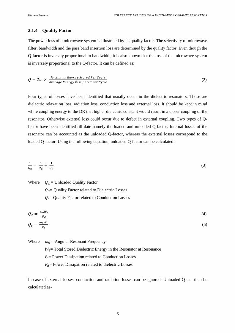
2.1.4 Quality Factor
The power loss of a microwave system is illustrated by its quality factor. The selectivity of microwave
filter, bandwidth and the pass band insertion loss are determined by the quality factor. Even though the
Q-factor is inversely proportional to bandwidth, it is also known that the loss of the microwave system
is inversely proportional to the Q-factor. It can be defined as:
(2)
Four types of losses have been identified that usually occur in the dielectric resonators. Those are
dielectric relaxation loss, radiation loss, conduction loss and external loss. It should be kept in mind
while coupling energy to the DR that higher dielectric constant would result in a closer coupling of the
resonator. Otherwise external loss could occur due to defect in external coupling. Two types of Q-
factor have been identified till date namely the loaded and unloaded Q-factor. Internal losses of the
resonator can be accounted as the unloaded Q-factor, whereas the external losses correspond to the
loaded Q-factor. Using the following equation, unloaded Q-factor can be calculated:
(3)
Where = Unloaded Quality Factor
= Quality Factor related to Dielectric Losses
= Quality Factor related to Conduction Losses
(4)
(5)
Where = Angular Resonant Frequency
= Total Stored Dielectric Energy in the Resonator at Resonance
= Power Dissipation related to Conduction Losses
= Power Dissipation related to dielectric Losses
In case of external losses, conduction and radiation losses can be ignored. Unloaded Q can then be
calculated as-

Khawar Naeem TOLERANCE ANALYSIS OF A MULTI-MODE CERAMIC RESONATOR
7
(6)
Where = Loss tangent of the resonator [14].
2.1.5 Resonant Frequency
Resonant frequency of a dielectric resonator is one where the stored magnetic and electric energies are
equal to each other. Minimum pass band insertion loss occurs at the instant when electromagnetic
energy is transferred to the load at resonant frequency. Both the resonant frequencies and spurious
modes of a dielectric resonator are a key factor when designing a DR filter. In order to design a DR
filter, fundamental and spurious mode resonant frequency has to be calculated beforehand [15].
The resonant frequencies of a dielectric resonator can be approximated by previously developed
models like Cohn’s and Itoh and Rudokah’s models [4]. All these models are subjected to limitations
in calculation accuracy of the resonant frequency. This presents the need to develop more robust and
accurate methods for the design of DR cavities and DR filters that are capable of including the effects
of surrounding environment of a DR also. For this reason, many iterative techniques have been
formulated to evaluate the exact solution by numerous approximations converging to the exact
solution. These techniques enable us to calculate the field strengths and resonant frequencies to a
certain accuracy level. Such techniques include mode matching method, finite element method and the
method of moments [16].
2.1.6 Tuning
In case of a dielectric resonator, operating frequency is dependent on resonator material permittivity
and its shape. One can tune the center frequency of the dielectric resonator in various ways. By design
or by putting an extra disk on top of the DR, one can fine tune the center frequency. Up to 15% change
can be achieved just by putting an extra tuning disk [17]. Tuning screws are used to mount the tuning
disk in the cavity. Frequency is affected in opposite direction when metallic disks are used instead of
the dielectric tuning disks. Dielectric tuning disks faces a reverse action when the DR fast approaches
the metallic disk resonant frequency. But additional tuning disks can have a negative impact on the Q
factor of the resonator, as it downgrades the Q value. Still, acceptable frequency response can be
achieved with this method. To overcome this issue, dielectric or metallic disks are mounted on screws
[3]. Certain frequencies can be obtained by turning the screw inwards or outwards. Mode of the
resonator and the desired tuning amount will define exactly which method to put into practice for this
instance [17].

Khawar Naeem TOLERANCE ANALYSIS OF A MULTI-MODE CERAMIC RESONATOR
8
2.1.7 Coupling
Energy is required to be coupled in or out of the resonators, in order for dielectric resonators to work
efficiently. There are several ways to do so such as waveguides transmission lines or electric and
magnetic coupling. The amount of coupling required or the resonator mode are determining factors for
coupling [5]. Magnetic coupling is the chosen solution for a cylindrical dielectric resonators operating
in mode. Apart from that, higher order filters can be achieved by coupling energy among
resonators. Direct coupling among resonators can be achieved by changing the resonator proximity.
Size and distance among resonators are defining factors for resonator coupling [5]. Several factors
such as the mode to be excited and transmission medium; should be taken into consideration while
choosing an appropriate structure to couple energy [17].
Coupling among the resonators is identified through strongest external field. Iris, an aperture within
the common wall of cavities is used to initiate coupling among resonators. Dimensions of iris are
changed frequently in order to attain varying coupling between resonators. Apart from iris, coupling
screws are used too.
2.1.8 Metallic Cavity
Radiation loss from a resonator can be overcome by adding a metallic cavity to the resonator. Cavity
dimension can also affect the response of the filter. Additionally, it can also affect the spurious
performance, temperature stability or the pass band insertion loss. Relationship between the cavity and
the resonator’s operating frequency can be described with the help of following equation:
√ (7)
Where = Volume of Metallic Cavity
= Dielectric Permittivity
A better Q-factor can be achieved by a large cavity size, but then again, it puts a negative impact on
the structure’s resonant frequency. Decreased x- dimension of the resonator cavity results in decreased
Q-factor. As a result, there is a growing insertion loss and decreased stop band rejection [15].
2.1.9 Dielectric Resonators
Due to high permittivity, dielectric materials can confine electromagnetic energy. A dielectric
resonator is defined as a material having high dielectric constant and usually having a cylindrical
shape. Typical shape is called as “puck” and is shown in the figure below. Due to difference in
permittivity of dielectric resonators, they can sustain resonance and energy inside at resonant
frequency [18]. The aim of enclosure is to stop the radiation from getting leaked outside, and the
conduction of enclosure is not dependent on the contact of puck. Resonant frequency is strongly

Khawar Naeem TOLERANCE ANALYSIS OF A MULTI-MODE CERAMIC RESONATOR
9
affected by dielectric constant and dimensions of a puck. A common dielectric resonator structure is
shown as under:
Fig.3. Conventional cross-section of a typical dielectric resonator structure [1].
The fields outside the dielectric resonator decay quickly as it moves at the opposite direction of the
puck. Dielectric resonators are mostly consisting of cylindrical pucks and have high Q-factor. The
spurious free response of the resonator can be achieved by introducing a hole inside the puck. The
fundamental TE01 mode of dielectric resonator and other higher order modes can be separated with
the help of this procedure. Adjustable metal plates above the resonator are used to fine tune the
dielectric resonators [19]. Center frequency of a resonator depends on physical dimensions and can be
adjusted by setting proper size. Low loss tangent and good temperature stability are the benchmark of
dielectric resonators [19]. Additionally, resonator modes are quite sensitive towards the diameter of
the dielectric resonator [6]. One more key characteristic of dielectric resonator is the High Q-factor to
volume ratio [17]. Dielectric resonator can also act as magnetic monopole in fundamental where
the E- field circulates in resonator and outward propagation of magnetic field is observed. Spurious
free bandwidth, Q-factor and the resonant frequencies are the most important properties of the
dielectric resonator [1]. But these properties are dependent on several factors such as the materials
used in the dielectric resonator, its shape and the mode used.
2.1.10 Multi-Mode Dielectric Resonators
Microwave resonators can be classified as single or multi-mode resonators. In a single mode resonator,
a singular field distribution is observed at the resonant frequency while in a dual mode resonator, we
have two field distributions at the desired resonant frequency and so on. The main reason for the usage
of multi-mode operation is size reduction as a single physical resonator is loaded with multiple
electrical resonators each having its own mode distribution. The multi-mode operation such as in dual
and triple mode resonators having multiple field distributions at the same frequency is generally due to
the degeneracy of the modes. These different field distributions in degenerate modes are mostly
orthogonal modes of a specific field distribution and arise due to symmetry of the resonator structure.
For this reason, 90-degree radial symmetry is generally used to realize dual mode resonators [20]

Khawar Naeem TOLERANCE ANALYSIS OF A MULTI-MODE CERAMIC RESONATOR
10
while triple mode operation is observed in cubic cavities or circular cavities with specific modes, [21]
,[22] and [23]. The following figure shows example of a dual, triple and quadruple-mode filters in
various technologies.
Fig.4. (left) Dual-Mode Micro-strip Filter [24], (middle) Waveguide Triple-Mode Filter [21], (right) Quadruple-
Mode Cavity in Circular waveguide [22]
The idea behind the multi-mode operation of dielectric resonators is the benefit in size reduction vital
for applications such as satellite communication systems but it also has some limitations. Even though
dielectric resonators can come in many shapes and forms, not all of them are easy to manufacture. The
main reason is the high pressure and temperature requirements needed while firing the ceramic.
In this thesis work, we will be focusing mainly on the dual mode resonator with emphasis on rigorous
analysis of the resonator structure in order to characterize the dual mode response.
2.2 Filters & Their Types
Filters are tasked with shaping the amplitude of the transmitted signals in most applications. But, time
delay or the linearity of insertion phase is highly important in some applications [13].
Filters are classified in several groups based on their frequency selectivity. Some of them are listed
below-
1. Low-pass filters: These filters are tasked with overseeing the transmission of low frequencies
from DC to a specific frequency. Here attenuation level is kept to a minimum (Fig. 8.a).
2. High-pass filters: These filters are tasked with transmitting signals above the cutoff frequency.
Anything below the cutoff frequency gets rejected (Fig. 8.b).

Khawar Naeem TOLERANCE ANALYSIS OF A MULTI-MODE CERAMIC RESONATOR
11
3. Band-pass filters: These filters only transmit a specific band of frequency. Anything below or
higher gets rejected (Fig. 8.c).
4. Band-stop filters: These filters are tasked with eliminating a specific band of frequency out of
a frequency spectrum (Fig. 8.d).
Fig. 5. Filter Types w.r.t Frequency selectivity [25]
Here, , , , and the are considered as the corner frequency of both low-pass and high-pass
filters, upper corner frequencies of band-pass and band-stop filters and pass band and stop band center
frequency respectively.
2.3 Two Port Network Theory
2.3.1 Y & Z-Parameters
The voltages and currents are directly related to each other by virtue of impedances or admittances, as
depicted in the two port network illustrated in figure below. The voltages can be calculated by Z-
parameters using the following equation, where it is represented in terms of currents.

Khawar Naeem TOLERANCE ANALYSIS OF A MULTI-MODE CERAMIC RESONATOR
12
V1= Z11I1 + Z12I2 (8)
V2 = Z21I1 + Z22I2 (9)
Fig. 6. A two-port network
On the other hand, in the form of matrices, it can be best illustrated with the help of following
equation:
[
]= [
] [
] (10)
The Z- matrices come in handy when portraying systems where networks are connected in series
rather than in shunts. Like this, linkage between currents and voltages through Y- parameters can be
described with the help of following equation:
I1 = Y11V1+ Y12V2 (11)
I2 = Y21V1 + Y22V2 (12)
While describing it in matrices, following equation can be used:
[
] = [
] [
] (13)
Unlike the Z- matrices, Y-matrices are of great use when portraying systems where networks are
connected in shunt.
2.3.2 ABCD-Parameters
If the two port networks are connected in cascade then ABCD parameters could possibly have a telling
impact on the systems. In order to calculate the overall ABCD matrix for the whole system, one would
have to calculate the matrix for a single two- port network first, and then multiply the calculated
amount with the total number of two-port networks.

Khawar Naeem TOLERANCE ANALYSIS OF A MULTI-MODE CERAMIC RESONATOR
13
The ABCD parameters, while working with a two-port network, can be described using the following
equation:
V1= AV2 + BI2 (14)
I1= CV2 + DI2 (15)
Additionally, in the form of matrices it can illustrated as depicted below-
[
]= [
] [
]
2.3.3 S-Parameters
Even though, Y- and Z- parameters are enough to describe most networks; sometimes it’s hard to
analyze a network using these parameters. Y & Z- parameters are used for low frequency networks
mostly since direct measurement of those parameters at high frequency could be troublesome. Two
factors are held responsible for such behavior:
1. In case of non- TEM transmission lines, it might be quite difficult to define the voltages and
currents at high frequencies.
2. It is of utmost importance to use open and short circuits while formulating those parameters.
But, it may cause instability to the system while working at microwave frequencies, especially
applicable if active elements are involved there.
While defining parameters, it is thought to have a relation with power which much unlike, can be
measured at high frequencies. In case of a two port network, the S- parameters are illustrated with a
and b waves representing the forward and reverse travelling waves respectively as shown in the figure
below.
Fig. 7. A two-port network characterized by S-parameters.
B1= S11a1 + S12a2 (16)
Khawar Naeem TOLERANCE ANALYSIS OF A MULTI-MODE CERAMIC RESONATOR
14
B2= S21a1+ S22a2 (17)
In the form of matrices:
[
]= [
] [
] (18)
If b2 in port 1 is calculated as zero, then S11 can be considered as the reflection coefficient. But for this
to happen, a perfectly matched load and the absence of source at the port 2 are pre-requisites. Same
formula is applicable for S22 where the b1 is absent.

Khawar Naeem TOLERANCE ANALYSIS OF A MULTI-MODE CERAMIC RESONATOR
15
3 Process & Results
The problem statement given at hand was to develop a routine for characterization of a dual mode
ceramic resonator inside a test cavity. To solve this problem, the solution process was divided into
various steps to achieve the required target. Following steps were included in the solution process:
Optimized EM design in HFSS
Detailed tolerance analysis
Equivalent circuit model in ADS
Test cavity Setup
Establish circuit-geometry correlation
MATLAB routine
The first step was to achieve the optimized EM design model of the dual mode ceramic resonator in
HFSS. The design process was initiated with single mode dielectric resonator and was then progressed
to the dual mode dielectric resonator. In the last part, a perturbation in the form of a diagonal cut was
introduced to achieve the desired coupling bandwidth.
The next step was to perform the tolerance analysis of the resonator models developed in the HFSS
environment. Test cases were setup to model different geometric tolerance scenarios and results were
recorded. The tolerance analysis was performed over the entire design work done during our research
so all the resonator models (single mode, dual mode and dual mode with coupling bandwidth) as well
as the test cavity models ( with reference resonator both lossless and with losses) were subjected to
tolerance analysis to come up with specifications of our resonator designs.
The next step was to develop the equivalent circuit models in ADS that exhibit the same response as
our EM models from HFSS. Coupled resonators circuit design were implemented to emulate the EM
response from HFSS and key circuit parameters such as inductor and capacitor values as well as
coupling coefficients and losses were extracted.
The process carried on the with the design on test cavity and coupling probes as well as a test case
(band-pass filter) to test the resonator in the test cavity. Both lossless and loss bearing simulations
were performed with the reference resonator inside the test cavity and sniffing probes and tolerance
analysis values were recorded. Equivalent circuit models were developed and circuit-geometry
correlation was established.

Khawar Naeem TOLERANCE ANALYSIS OF A MULTI-MODE CERAMIC RESONATOR
16
In the last part, MATLAB routine was developed based on the circuit solution of the equivalent circuit
models created hence eliminating the need for the use of circuit simulator and a robust solution was
achieved to specify the dual mode resonator inside test cavity. The routine was thoroughly tested for
different cases of tolerance analysis and conclusions were drawn based on the performance of routine
in different scenarios.
In the next section, all the results during the design work are presented. The results breakdown is
given as under:
Empty cavity analysis
Single mode DR & tolerance analysis
Dual mode DR & tolerance analysis
Dual mode DR with diagonal cut & tolerance analysis
Circuit-geometry correlation (along with band-pass filter test case & coupling probes)
Test cavity with reference resonator (With & Without losses & tolerance analysis)
MATLAB routine
3.1 Results
3.1.1 HFSS Simulations of TM Mode Dielectric Resonator
In order to come up with the optimal dimensions of the dual-mode dielectric resonator, HFSS
simulations were performed. HFSS is a simulation tool that employs the Finite Element Method
(FEM) to obtain a complete three dimensional electromagnetic field inside a respective structure.
Using this electromagnetic field solution, HFSS can then calculate S-parameters. HFSS was employed
in this thesis project to determine the resonant frequencies of the dielectric resonator inside the test
cavity.
3.1.2 Empty Cavity
Simulations were undertaken for a cavity size of 30*30*30 (mm) without the addition of losses and
with the addition of losses to characterize the general behavior of the test cavity. The first two modes
above 1GHz were calculated for both cases. Losses were calculated for the cavity by assigning finite
conductivity of the value (S/m).

Khawar Naeem TOLERANCE ANALYSIS OF A MULTI-MODE CERAMIC RESONATOR
17
Fig.8. Empty cavity
The HFSS simulation results from the Eigen-mode solution are given as under:
Cavity
Mode 1
Frequency
(MHz)
Mode 2
Frequency
(MHz)
Mode 3
Frequency
(MHz)
Without Losses 7066.43 7066.69 7066.76
With Losses 7065.98 7066.23 7066.38
Table 1. Eigen-mode data from the empty cavity simulation
The Eigen-mode solution from HFSS with number of modes set to 3 returns us the values shown in the
table above. The little frequency shift observed in the three modes inside the empty cavity is due to
numerical inaccuracy of the simulation software which implies that in reality all these three modes are
resonating at the same frequency but due to error tolerance of HFSS Eigen-mode solver these three
frequencies are few kHz apart.
3.1.3 Single Mode DR
A single Mode Dielectric resonator puck was placed inside the test cavity having dimensions
8.3*8.35*30 mm and dielectric constant = 35 and no losses i.e. tan = 0 to obtain a resonant
frequency of 1960 MHz

Khawar Naeem TOLERANCE ANALYSIS OF A MULTI-MODE CERAMIC RESONATOR
18
Fig.9. Single mode DR inside test cavity
The following resonant frequency was obtained with the Eigen mode solution.
Case Mode 1 Frequency (MHz)
Single Mode DR 1960.19
Table 2. Eigen-mode data for single mode DR inside test cavity
3.1.3.1 Electric & Magnetic Field Distribution TM01 Mode
The electric field and the magnetic field distributions inside the single mode DR are given as under:
Fig.10. E-field & H-field for TM01 mode for a single mode DR
We can observe from the above figures that the electric field strength is concentrated inside the
dielectric puck whereas magnetic field is perpendicular to that of the electric field strength for the
single mode resonant frequency. To understand the TM01 mode operation, key references are Rebsch
[9], Kobayashi [10], and Zaki et al. [8] and [11].
3.1.3.2 Tolerance Analysis (Width & Thickness)
The next step was to run the geometry tolerance analysis for the single mode DR to observe its
behavior relative to the change in geometry. Two simulations were setup each for thickness and width
tolerance and its effect on the resonant frequencies was observed.
Fig.11. Tolerance Setup for single mode DR
The following resonant frequencies were obtained during the geometry tolerance analysis:
Khawar Naeem TOLERANCE ANALYSIS OF A MULTI-MODE CERAMIC RESONATOR
19
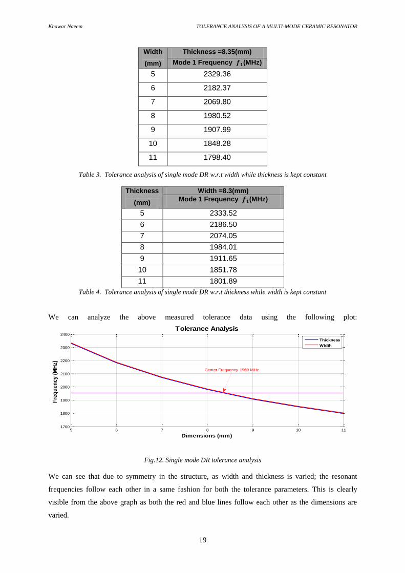
Width
(mm)
Thickness =8.35(mm)
Mode 1 Frequency (MHz)
5 2329.36
6 2182.37
7 2069.80
8 1980.52
9 1907.99
10 1848.28
11 1798.40
Table 3. Tolerance analysis of single mode DR w.r.t width while thickness is kept constant
Thickness
(mm)
Width =8.3(mm)
Mode 1 Frequency (MHz)
5 2333.52
6 2186.50
7 2074.05
8 1984.01
9 1911.65
10 1851.78
11 1801.89
Table 4. Tolerance analysis of single mode DR w.r.t thickness while width is kept constant
We can analyze the above measured tolerance data using the following plot:
Fig.12. Single mode DR tolerance analysis
We can see that due to symmetry in the structure, as width and thickness is varied; the resonant
frequencies follow each other in a same fashion for both the tolerance parameters. This is clearly
visible from the above graph as both the red and blue lines follow each other as the dimensions are
varied.
5 6 7 8 9 10 111700
1800
1900
2000
2100
2200
2300
2400
Dimensions (mm)
Fre
qu
en
cy (
MH
z)
Tolerance Analysis
Thickness
Width
Center Frequency 1960 MHz

Khawar Naeem TOLERANCE ANALYSIS OF A MULTI-MODE CERAMIC RESONATOR
20
3.1.4 Dual Mode DR
A cross-shaped dual-mode resonator puck was placed inside the test cavity with dimensions
8*7.92*30 mm having dielectric constant = 35 and no losses i.e. tan = 0 to obtain a resonant
frequency of 1960 MHz.
Fig.13. Dual-mode DR inside test cavity
The Eigen-Mode analysis generated the following resonant frequencies:
Case Mode 1 Frequency
(MHz)
Mode 2 Frequency
(MHz)
Dual- Mode DR 1960.52 1960.55
Table 5. Eigen-mode data for Dual mode DR inside test cavity
3.1.4.1 Electric & Magnetic Field Distribution for two orthogonal TM01 Modes
The electric field and magnetic field distributions inside the dual-mode DR for both the modes are
given as following:
(a) (b)

Khawar Naeem TOLERANCE ANALYSIS OF A MULTI-MODE CERAMIC RESONATOR
21
(c) (d)
Fig.14. (a) TM01 Mode1 E-field (b) TM01 Mode1 H-field (c) TM01 Mode 2 E-field (d) TM 01 Mode 2 H-field
The field plots of the two TM01 modes above indicate that we have two orthogonal modes inside the
test cavity and the two resonant frequencies are only few kHz apart which as explained earlier is due
to error tolerance inherent in the Eigen-mode solver of HFSS.
3.1.4.2 Tolerance Analysis
The tolerance analysis is one of the key steps in specification of a resonator. The principle behind
tolerance analysis is to test and check as to how different a resonator can behave if its geometry is
subjected to manufacturing tolerances in terms of width, thickness, dielectric constant and other
geometric tolerances. These tolerances affect the resonating frequency as well as coupling coefficient
and other parameters related to the resonator and hence need to be tested and specified. The geometry
tolerance analysis was also performed on the dual-mode resonator to see the behavior of resonant
frequencies with changing physical dimensions. In the first step, two simulations (test cases) were
performed each for the thickness and width of the dielectric resonator while keeping the nominal value
intact for a given iteration.
Fig. 15. Tolerance Setup for Dual mode DR

Khawar Naeem TOLERANCE ANALYSIS OF A MULTI-MODE CERAMIC RESONATOR
22
Table 6. Tolerance analysis of Dual-mode DR w.r.t width while thickness is kept constant
Table 7. Tolerance analysis of Dual-mode DR w.r.t width while thickness is kept constant
The following trend was seen when the above recorded tolerance data was analyzed in the form of
respective dimensions versus frequency plot.
Fig.16. Dual-Mode DR tolerance analysis
5 6 7 8 9 10 111700
1800
1900
2000
2100
2200
2300
2400
Dimensions (mm)
Fre
qu
en
cy (
MH
z)
Dual Mode DR Tolerance Analysis
Thickness
Width
Center Frequency 1960 MHz
Width
(mm)
Thickness =7.92(mm)
Mode 1 Frequency
(MHz)
Mode 2 Frequency
(MHz)
5 2317.55 2317.70
6 2166.30 2166.63
7 2051.44 2051.72
8 1960.52 1960.55
9 1886.92 1887.01
10 1826.48 1826.53
11 1777.73 1777.85
Thickness
(mm)
Width =8(mm)
Mode 1 Frequency
(MHz)
Mode 2 Frequency
(MHz)
5 2301.98 2302.12
6 2156.28 2156.30
7 2042.20 2042.34
8 1954.24 1954.38
9 1882.52 1882.58
10 1823.47 1823.55
11 1774.51 1774.59

Khawar Naeem TOLERANCE ANALYSIS OF A MULTI-MODE CERAMIC RESONATOR
23
We can observe from the above plot the tolerance w.r.t both width and thickness. We can see that for
the smaller dimension size such as 5mm, the dual mode frequencies are significantly apart but as we
increase the dimension size, the dual-mode frequencies start to vary in a more synchronous manner for
both the tolerance parameters.
The next step was to check the tolerance against the dielectric constant of the dual-mode resonator.
The case for change in dielectric constant was setup as we have various materials provided by the
manufacturers with different dielectric constants, quality factor and cost. Based on the data collected
during this tolerance analysis, a dielectric material will be chosen for use in the dual mode case. HFSS
simulations were setup for the nominal values of thickness and width at center frequency of 1960
MHz and the following data was recorded.
Dielectric
Constant
Mode 1 Frequency
(MHz)
Mode 2 Frequency
(MHz)
Step Size
/
(MHz)
33 2018.07 2018.17 57.55/57.62
34 1989.66 1989.70 29.14/29.15
35 1960.52 1960.55 0
36 1934.25 1934.46 26.27/26.09
37 1909.09 1909.20 51.43/51.35
Table 8. Tolerance analysis of Dual mode DR w.r.t dielectric constant
3.2 Dual-Mode DR with diagonal cut
During the course of the design work in HFSS, several resonator models were created to intentionally
destroy the symmetry of the resonator and separate the two resonant frequencies and generate coupling
bandwidth between the two modes. Several geometries were designed and simulated but at the end the
single diagonal two-cut variant of the dual-mode DR was finalized. The dimensions of dual-mode DR
were adjusted to 8*8.2*30 mm with 1*1 cut area.
Fig.17. (a) Dual Mode DR with diagonal cut (b) Dual Mode DR with diagonal Cut Setup

Khawar Naeem TOLERANCE ANALYSIS OF A MULTI-MODE CERAMIC RESONATOR
24
Cut
Width
(mm)
Cut
Length
(mm)
Even Mode
Frequency
(MHz)
Center
Frequency
(MHz)
Odd Mode
Frequency
(MHz)
Coupling
Factor
k=[
]
1 1 1943.83 1960.47 1977.11 0.016
Table 9. Eigen-mode data for Dual mode DR with coupling bandwidth
The electric and magnetic field distribution inside the cut variant of dual-mode DR can be seen as
under:
(a) (b)
(c) (d)
Fig.18. (a) Even Mode E-field (b) Even Mode H-field (c) Odd Mode E-field (d) Odd Mode H-field
We can see from the electric and magnetic field plots above that the symmetry of both the fields
within the test cavity has been destroyed and the two modes are not perfectly orthogonal to each other
as before giving rise to two different resonant frequencies and a coupling bandwidth of 33.28 MHz
was observed for a cut area of 1*1 These modes are termed as even and odd modes and have
been generated due to perturbation of the resonator by the diagonal cut. To read in detail about the
even and odd mode theory, reference Cameron [27] is highly useful.

Khawar Naeem TOLERANCE ANALYSIS OF A MULTI-MODE CERAMIC RESONATOR
25
The next step was to perform tolerance analysis for the cut variant of the dual-mode DR. The tolerance
analysis included thickness and width tolerance, dielectric tolerance, cut length, cut width and cut
offset tolerance. Simulations were setup for each case; for the eigen mode analysis of every parameter.
Following are the results for the Eigen-mode simulations for different tolerance parameters:
Table 10. Eigen-mode data for tolerance analysis of Dual mode DR with coupling bandwidth w.r.t thickness
while width is kept constant
Table 11. Eigen-mode data for tolerance analysis of Dual mode DR with coupling bandwidth w.r.t width while
thickness is kept constant
The next step was to check the tolerance against the dielectric constant of the dual-mode resonator.
HFSS simulations were setup for the nominal values of thickness and width at center frequency of
1960 MHz and the following data was recorded.
Thickness
(mm)
Width =8(mm)
Even Mode
Frequency
(MHz)
Odd Mode
Frequency
(MHz)
Coupling
Factor
k=[
]
Center
Frequency
(MHz)
8 1959.47 1992.87 0.0169 1976.17 8.1 1951.33 1984.81 0.0170 1968.07 8.2 1943.83 1977.11 0.0169 1960.47 8.3 1936.17 1969.30 0.0169 1952.73 8.4 1928.64 1961.35 0.0168 1944.99
Width
Thickness =8.2(mm)
Even Mode
Frequency
(MHz)
Odd Mode
Frequency
(MHz)
Coupling
Factor
k=[
]
Center
Frequency
(MHz)
7.8 1960.04 1989.45 0.0148 1974.74
7.9 1951.83 1983.15 0.0159 1967.49
8 1943.83 1977.11 0.0169 1960.47
8.1 1935.86 1970.91 0.0179 1953.38
8.2 1925.42 1962.63 0.0191 1944.02

Khawar Naeem TOLERANCE ANALYSIS OF A MULTI-MODE CERAMIC RESONATOR
26
Table 12. Eigen-mode data for tolerance analysis of Dual mode DR with coupling bandwidth w.r.t dielectric
constant
The next simulation that was carried out was the tolerance of the cut variant of the dual-mode DR with
cut width and cut length as the respective parameters. The following values were recorded:
Table 13. Eigen-mode data for tolerance analysis of Dual mode DR with coupling bandwidth w.r.t cut
width while cut length is kept constant
Table 14. Eigen-mode data for tolerance analysis of Dual mode DR with coupling bandwidth w.r.t cut width
while cut length is kept constant
Cut
Width
(mm)
Cut Length = 1(mm)
Even Mode
Frequency
(MHz)
Odd Mode
Frequency
(MHz)
Coupling
Factor
k=[
]
Center
Frequency
(MHz)
0.8 1942.86 1973.47 0.0156 1958.16
0.9 1943.04 1975.26 0.0164 1959.15
1 1943.83 1977.11 0.0169 1960.47
1.1 1944.25 1978.75 0.0175 1961.50
1.2 1944.84 1980.32 0.0180 1962.58
Dielectric
Constant
Even Mode
Frequency
(MHz)
Odd Mode
Frequency
(MHz))
Coupling
Factor
k=[
]
Center
Frequency
(MHz)
Step Size
/
(MHz)
33 1999.48 2033.36 0.0168 2016.42 55.65/56.25
34 1971.08 2004.62 0.0168 1987.57 27.25/27.51
35 1943.83 1977.11 0.0169 1960.47 0
36 1917.71 1950.70 0.0170 1934.20 26.12/26.41
37 1892.59 1925.32 0.0171 1908.95 51.24/51.79
Cut Length
(mm)
Cut Width = 1(mm)
Even Mode
Frequency
(MHz)
Odd Mode
Frequency
(MHz)
Coupling
Factor
k=[
]
Center
Frequency
(MHz)
0.8 1943.09 1969.70 0.0136 1956.39
0.9 1943.51 1973.48 0.0153 1958.49
1 1943.83 1977.11 0.0169 1960.47
1.1 1944.20 1980.94 0.0187 1962.57
1.2 1944.34 1984.67 0.020 1964.50

Khawar Naeem TOLERANCE ANALYSIS OF A MULTI-MODE CERAMIC RESONATOR
27
All the above data was recorded, the change in frequencies and coupling coefficient was observed for
the different cases and based on these values the manufacturing tolerances will be specified when
placing the order for commercial units of the resonator from ceramic manufacturers.
3.3 Circuit-Geometry Correlation
3.3.1 Coupling Probes
To couple electromagnetic energy to the modes inside the test cavity with a dielectric resonator,
coupling probes are required. For this purpose, two kinds of probes are generally used: electric and
magnetic loops. Different coupling probes were tested during the entire thesis period to couple the
energy efficiently to the two modes inside the test cavity and at the end, magnetic square loop was
finalized, because of its efficiency and ease of manufacturing in future.
Fig. 19. Magnetic Square Loop
3.3.2 Single Mode DR
To characterize the resonator, equivalent circuit models were created to establish the correlation
between circuit and geometry. For this purpose, ADS (Advanced Design System) software was
employed to create circuit models and simulate the circuit models. The following HFSS and circuit
(ADS) model was created for the single mode DR.
Fig. 20. Single mode DR inside test cavity with coupling probes
The lumped element equivalent circuit model for the single mode DR is given as under:
Khawar Naeem TOLERANCE ANALYSIS OF A MULTI-MODE CERAMIC RESONATOR
28
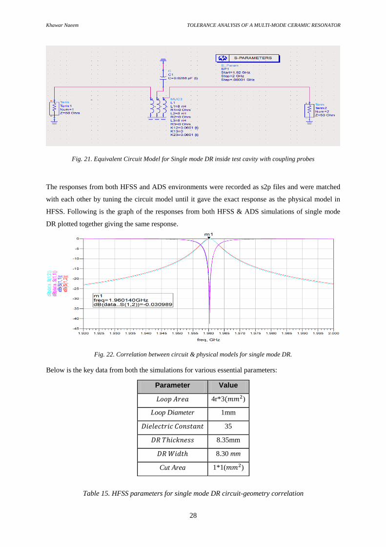
Fig. 21. Equivalent Circuit Model for Single mode DR inside test cavity with coupling probes
The responses from both HFSS and ADS environments were recorded as s2p files and were matched
with each other by tuning the circuit model until it gave the exact response as the physical model in
HFSS. Following is the graph of the responses from both HFSS & ADS simulations of single mode
DR plotted together giving the same response.
Fig. 22. Correlation between circuit & physical models for single mode DR.
Below is the key data from both the simulations for various essential parameters:
Table 15. HFSS parameters for single mode DR circuit-geometry correlation
Parameter Value
4r*3 )
Loop Diameter 1mm
35
8.35mm
8.30 mm
Cut Area 1*1( )

Khawar Naeem TOLERANCE ANALYSIS OF A MULTI-MODE CERAMIC RESONATOR
29
Table 16. ADS parameters for single mode DR circuit-geometry correlation (from equivalent circuit)
3.3.3 Dual Mode DR with Diagonal Cut
After completing the correlation between circuit and physical model for the single mode DR, the same
method was applied for dual mode DR as well. Coupling probes were used to couple the energy to the
two orthogonal modes inside the test cavity. Since filters are used to define the geometry of a
resonator, as a test case, two band-pass filters with 20 dB return loss specification were developed: one
using the inductive (magnetic) coupling probes and other with the capacitive (electric) coupling
probes.
3.3.3.1 Band-pass Filter Test Case (Inductive Coupled)
Since filters are used to define the geometry of a resonator, an inductive coupled band-pass filter was
developed as a part of characterizing the dual mode resonator inside the test cavity. Magnetic probes
were used to achieve strong coupling between input/output and the two modes inside the cavity and
band-pass response was generated.
Fig. 23. Band-pass filter test case (inductive coupled) for dual mode DR
The equivalent circuit model obtained for the dual mode inductive coupled case is given as under:
Parameter Value
0.0601
0.0601
8nH
0.8288pF

Khawar Naeem TOLERANCE ANALYSIS OF A MULTI-MODE CERAMIC RESONATOR
30
Fig. 24. Equivalent circuit model of band-pass filter test case (inductive coupled) for dual mode DR
Responses of both the HFSS and ADS models were recorded in the form of s2p files and plotted
together and the circuit model was tuned to get the exact same response as the physical mode for dual
mode DR. Following figure contains both HFSS & ADS responses plotted together:
Fig. 25. Correlation between circuit & physical models for dual mode DR w.r.t band-pass filter test
case (inductive coupled).
The important parameters of both the HFSS model and ADS model are listed as under:
Table 17. HFSS parameters for dual mode DR circuit-geometry correlation w.r.t band-pass filter test
case (inductive coupled)
Parameter Value
9.5r*9.2 )
Loop Diameter 1mm
35
8.7mm
8.6 mm
Cut Area 1*1( )

Khawar Naeem TOLERANCE ANALYSIS OF A MULTI-MODE CERAMIC RESONATOR
31
Table 18. ADS parameters for dual mode DR circuit-geometry correlation w.r.t band-pass filter test
case (inductive coupled)
3.3.3.2 Band-pass Filter Test Case (Capacitive Coupled)
Similar method was used to generate the band-pass filter test case with capacitive (electric) probes.
Electric probes were created to couple energy efficiently to the two resonant modes inside the test
cavity to give rise to the band-pass filter response.
Fig. 26. Band-pass filter test case (capacitive coupled) for dual mode DR
The equivalent circuit model was created in ADS which is given as under:
Fig. 27. Equivalent circuit model of Band-pass filter test case (capacitive coupled) for dual mode DR
Parameter Value
0.0247
0.2400
0.2400
8nH
0.864 pF

Khawar Naeem TOLERANCE ANALYSIS OF A MULTI-MODE CERAMIC RESONATOR
32
Both models were simulated and there results were exported as s2p files which were then used to
correlate both of them by tuning the circuit model. Here are the results for the correlated responses of
both the models:
Fig. 28. Correlation between circuit & physical models for dual mode DR w.r.t band-pass filter test case
(capacitive coupled).
Important parameters of both the models for this test case are tabulated as:
Table 19. ADS parameters for dual mode DR circuit-geometry correlation w.r.t band-pass filter test case
(capacitive coupled)
Table 20. HFSS parameters for dual mode DR circuit-geometry correlation w.r.t band-pass filter test
case (capacitive coupled)
Parameter Value
0.015
& 0.138pF
8nH
0.687 pF
Parameter Value
12.5mm
Loop Diameter 1mm
35
8 mm
8 mm
Cut Area 1*1( )

Khawar Naeem TOLERANCE ANALYSIS OF A MULTI-MODE CERAMIC RESONATOR
33
3.4 Test Cavity
The next step in the process was to characterize the test cavity for the dual mode DR. For this purpose,
the reference resonator from the inductive coupled band-pass filter test case was put inside the test
cavity and weak coupling probes (sniffers) were used to measure the test cavity response. A circuit
model was created for the test cavity as the first step and then a detailed tolerance analysis was
performed with several parameters on the reference resonator inside the test cavity.
Fig. 29. Test cavity with reference resonator & sniffing probes
3.4.1 Reference Resonator
The reference resonator has been picked up from the inductive coupled two pole bandpass filter test
case and has been placed inside the test cavity to analyze its behavior. The reference resonator
parameters are given as under:
Table 21. Reference Resonator Parameters
3.4.2 Circuit Model & Correlated Response
Just like the previous cases, an equivalent circuit model was developed in ADS to specify the test
cavity response with weak coupling probes and the reference resonator. Following figure shows the
equivalent circuit model developed in ADS for the test cavity.
Parameter Value
35
8.7 mm
8.6 mm
Cut Area 1*1( )

Khawar Naeem TOLERANCE ANALYSIS OF A MULTI-MODE CERAMIC RESONATOR
34
Fig. 30. Equivalent Circuit model for Test cavity with reference resonator & sniffing probes
The correlated response for both the HFSS and ADS models for the test cavity case is given by:
Fig. 31. Correlation between circuit & physical models for test cavity with reference resonator & coupling
probes
Several key parameters from both HFSS and ADS models are given in the tables below:
Table 22. HFSS parameters for test cavity circuit-geometry correlation
Parameter Value
2*1.5r )
Loop Diameter 1mm
Cavity Size 30*30*30 (mm)

Khawar Naeem TOLERANCE ANALYSIS OF A MULTI-MODE CERAMIC RESONATOR
35
Table 23. ADS parameters for test cavity circuit-geometry correlation
3.4.3 Tolerance Analysis
Detailed tolerance analysis was performed for the reference resonator inside test cavity w.r.t all the
different tolerance parameters such as thickness, width, dielectric constant variation, cut length, cut
width and cut offset.
The first simulation was tolerance analysis w.r.t thickness of the reference resonator. The limits for the
thickness tolerance were specified to be ±0.2mm. Here are the results recorded for the tolerance
simulation:
Fig. 32. Test cavity tolerance analysis setup w.r.t thickness
Cross
Thickness
(mm)
Even Mode
Frequency
(MHz)
Center
Frequency
(MHz)
Odd Mode
Frequency
(MHz)
Coupling
Factor
k=[
]
8.5 1873.41 1894.70 1915.99 0.0225
8.6 1866.09 1887.26 1908.43 0.0224
8.7 1859.41 1880.62 1901.83 0.0225
8.8 1852.77 1873.92 1895.08 0.0225
8.9 1846.17 1867.14 1888.12 0.0224
Table 24. Driven-modal data for test cavity tolerance analysis w.r.t thickness
Parameter Value
0.0225
0.0036
0.0036
8nH
0.8956 pF

Khawar Naeem TOLERANCE ANALYSIS OF A MULTI-MODE CERAMIC RESONATOR
36
Responses for each simulation was saved as an s2p file and were later on plotted together to see the
difference in test cavity response due to change in thickness of the reference resonator. Following
figure depicts the thickness tolerance clearly.
Fig. 33. Test cavity tolerance analysis w.r.t thickness
The next simulation was to do the tolerance analysis of the reference resonator w.r.t its width. The
limits specified for the width tolerance were same as thickness tolerance and following data was
recorded:
Fig. 34. Test cavity tolerance analysis setup w.r.t width
Khawar Naeem TOLERANCE ANALYSIS OF A MULTI-MODE CERAMIC RESONATOR
37
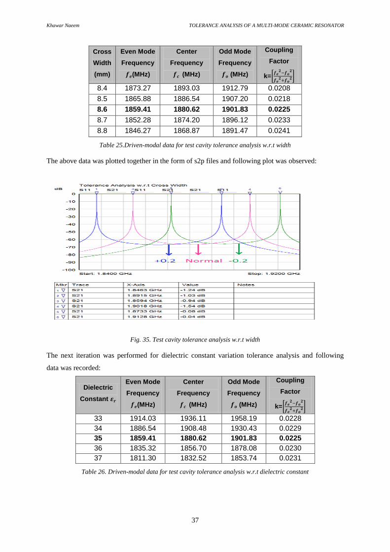
Cross
Width
(mm)
Even Mode
Frequency
(MHz)
Center
Frequency
(MHz)
Odd Mode
Frequency
(MHz)
Coupling
Factor
k=[
]
8.4 1873.27 1893.03 1912.79 0.0208
8.5 1865.88 1886.54 1907.20 0.0218
8.6 1859.41 1880.62 1901.83 0.0225
8.7 1852.28 1874.20 1896.12 0.0233
8.8 1846.27 1868.87 1891.47 0.0241
Table 25.Driven-modal data for test cavity tolerance analysis w.r.t width
The above data was plotted together in the form of s2p files and following plot was observed:
Fig. 35. Test cavity tolerance analysis w.r.t width
The next iteration was performed for dielectric constant variation tolerance analysis and following
data was recorded:
Dielectric
Constant
Even Mode
Frequency
(MHz)
Center
Frequency
(MHz)
Odd Mode
Frequency
(MHz)
Coupling
Factor
k=[
]
33 1914.03 1936.11 1958.19 0.0228
34 1886.54 1908.48 1930.43 0.0229
35 1859.41 1880.62 1901.83 0.0225
36 1835.32 1856.70 1878.08 0.0230
37 1811.30 1832.52 1853.74 0.0231
Table 26. Driven-modal data for test cavity tolerance analysis w.r.t dielectric constant

Khawar Naeem TOLERANCE ANALYSIS OF A MULTI-MODE CERAMIC RESONATOR
38
The above recorded data was plotted together in one plot resulting in the following figure:
Fig. 36. Test cavity tolerance analysis w.r.t dielectric constant
The next simulation sequence was the cut length tolerance. Limits were specified as same as the
thickness tolerance i.e. ±0.2mm and following results were obtained:
Fig. 37. Test cavity tolerance analysis w.r.t cut length

Khawar Naeem TOLERANCE ANALYSIS OF A MULTI-MODE CERAMIC RESONATOR
39
Cut
Length
(mm)
Even Mode
Frequency
(MHz)
Center
Frequency
(MHz)
Odd Mode
Frequency
(MHz)
Coupling
Factor
k=[
]
0.8 1859.03 1877.48 1895.93 0.0196
0.9 1859.34 1879.21 1899.08 0.0211
1 1859.41 1880.62 1901.83 0.0225
1.1 1859.65 1882.35 1905.06 0.0241
1.2 1859.63 1884.29 1908.96 0.0261
Table 27. Driven-modal data for test cavity tolerance analysis w.r.t cut length
Just like previous cases, all the relevant s2p files for the above data were plotted together as under:
Fig. 38. Test cavity tolerance analysis w.r.t cut length
The next simulation was done in the same fashion for cut width given as follows:
Fig. 39. Test cavity tolerance analysis w.r.t cut width
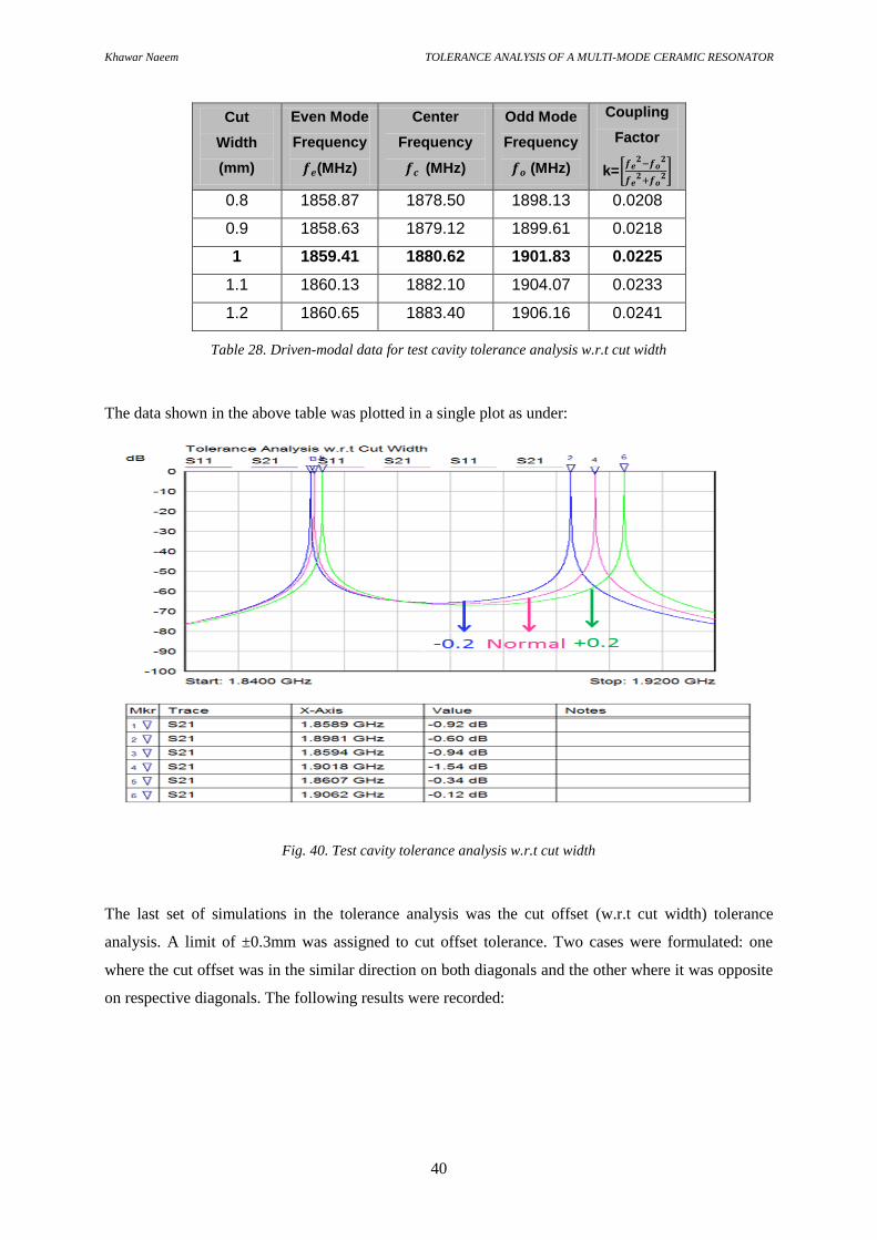
Khawar Naeem TOLERANCE ANALYSIS OF A MULTI-MODE CERAMIC RESONATOR
40
Cut
Width
(mm)
Even Mode
Frequency
(MHz)
Center
Frequency
(MHz)
Odd Mode
Frequency
(MHz)
Coupling
Factor
k=[
]
0.8 1858.87 1878.50 1898.13 0.0208
0.9 1858.63 1879.12 1899.61 0.0218
1 1859.41 1880.62 1901.83 0.0225
1.1 1860.13 1882.10 1904.07 0.0233
1.2 1860.65 1883.40 1906.16 0.0241
Table 28. Driven-modal data for test cavity tolerance analysis w.r.t cut width
The data shown in the above table was plotted in a single plot as under:
Fig. 40. Test cavity tolerance analysis w.r.t cut width
The last set of simulations in the tolerance analysis was the cut offset (w.r.t cut width) tolerance
analysis. A limit of ±0.3mm was assigned to cut offset tolerance. Two cases were formulated: one
where the cut offset was in the similar direction on both diagonals and the other where it was opposite
on respective diagonals. The following results were recorded:

Khawar Naeem TOLERANCE ANALYSIS OF A MULTI-MODE CERAMIC RESONATOR
41
Fig. 41. Test cavity tolerance analysis setup w.r.t cut offset (similar direction)
Cut Offset
(mm)
Even Mode
Frequency
(MHz)
Center
Frequency
(MHz)
Odd Mode
Frequency
(MHz)
Coupling
Factor
k=[
]
-0.3(up) 1860.50 1882.06 1903.63 0.0229
Normal 1859.41 1880.62 1901.83 0.0225
+0.3(down) 1860.04 1881.07 1902.11 0.0223
Table 29. Driven-modal data for test cavity tolerance analysis w.r.t cut offset (similar direction)
The above data was plotted in the following figure:
Fig. 42. Test cavity tolerance analysis w.r.t cut offset (similar direction)
For cut offset in the opposite direction, the following behavior was recorded:

Khawar Naeem TOLERANCE ANALYSIS OF A MULTI-MODE CERAMIC RESONATOR
42
Fig. 43. Test cavity tolerance analysis w.r.t cut offset (opposite direction)
Cut Offset
(mm)
Even Mode
Frequency
(MHz)
Center
Frequency
(MHz)
Odd Mode
Frequency
(MHz)
Coupling
Factor
k=[
]
Case 1 1859.47 1881.22 1902.97 0.0231
Normal 1859.41 1880.62 1901.83 0.0225
Case 2 1860.00 1881.95 1903.91 0.0233
Table 30. Driven-modal data for test cavity tolerance analysis w.r.t cut offset (opposite direction)
The following plot was observed when the data in the above table was plotted together:
Fig. 44. Test cavity tolerance analysis w.r.t cut offset (opposite direction)

Khawar Naeem TOLERANCE ANALYSIS OF A MULTI-MODE CERAMIC RESONATOR
43
3.4.4 Test Cavity with Reference Resonator & Losses
In the next simulation task, losses were added to the test cavity and resonator to see how the test cavity
response changes in the presence of losses. Three cases were developed in which first only the cavity
was changed to be having losses, then losses were added to resonator only and in the last case, both
cavity and resonator were modified to be as entities with losses.
For the first case, when cavity was modified to be having finite conductivity whereas the dielectric
material was ideal, we observed the following results:
Table 31. Parameters for the test cavity with losses
Even Mode
Frequency
(MHz)
Center
Frequency
(MHz)
Odd Mode
Frequency
(MHz)
Coupling
Factor
k=[
]
Mode 1
Q
Mode 2
Q
1863.43 1885.48 1907.53 0.0233 9946 8273
Table 32. Eigen-mode data for test cavity with losses
For the second case, reference resonator was modified to be the one with the losses and cavity was
assigned to be lossless. Following results came out as a result of that simulation:
Parameter Value
35
3.33 e-5
30000
Table 33. Parameters for the reference resonator with losses
Parameter Value
Silver
41000000(S/m)
35
8.7 mm
8.6 mm
Cut Area 1*1( )
Cavity Size 30*30*30( mm)

Khawar Naeem TOLERANCE ANALYSIS OF A MULTI-MODE CERAMIC RESONATOR
44
Even Mode
Frequency
(MHz)
Center
Frequency
(MHz)
Odd Mode
Frequency
(MHz)
Coupling
Factor
k=[
]
Mode 1
Q
Mode 2
Q
1863.12 1885.20 1907.28 0.0234 31143 31474
Table 34. Eigen-mode data for reference resonator with losses
The last case was setup such that both the cavity and resonator included losses. This case resulted in
the following results:
Even Mode
Frequency
(MHz)
Center
Frequency
(MHz)
Odd Mode
Frequency
(MHz)
Coupling
Factor
k=[
]
Mode 1
Q
Mode 2
Q
1863.52 1885.60 1907.69 0.0234 7811 6351
Table 35. Eigen-mode data for test cavity & reference resonator both with losses
3.4.5 Tuning Screw Simulation & Quality Factor
The tuning screw test case was setup in order to check if we can compensate the effect of geometric
(manufacturing tolerances) without compromising our quality factor too much. These values will give
us an idea of how much tuning range we have without destroying the quality factor. In the next
simulation sequence, a brass tuning screw of radius 1 mm was inserted from the top of the test cavity
while the cavity and resonator were both having losses as in the previous case. The quality factor Q
was observed for both the modes and is given as under:
Tuning
Distance
(mm)
Even Mode
Frequency
(MHz)
Center
Frequency
(MHz)
Odd Mode
Frequency
(MHz)
Coupling
Factor
k=[
]
Mode 1
Q
Mode 2
Q
1 1863.42 1886.06 1908.70 0.0240 7089 7246
2 1863.07 1886.59 1910.11 0.0249 7083 7150
3 1862.81 1887.56 1912.31 0.0262 7080 7049
4 1861.84 1887.90 1913.96 0.0276 7072 6931
5 1860.88 1888.26 1915.65 0.0289 7069 6846
Table 36. Eigen-mode data for tuning screw simulation for test cavity & reference resonator both with losses

Khawar Naeem TOLERANCE ANALYSIS OF A MULTI-MODE CERAMIC RESONATOR
45
4 MATLAB Routine
In the last part of the thesis work, a MATLAB routine was developed based on the ABCD-parameters
two port network solution of the equivalent circuit of the test cavity. Non-linear equations were
developed describing the equivalent circuit and ABCD to S-parameter conversion was performed to
get the response in terms of S-parameters to correlate with the circuit model. The complete set of non-
linear equations is given in Appendix A under the MATLAB code.
To find the three unknown of the system of non-linear equations, first the equations were made non-
dimensional. Constants like L, C, which are of order of nH are all divided by 1 ; frequency is
multiplied by 1 . By scaling these variables, unknowns will be of order, O(1). After getting non-
dimensional set of equations, parameters are solved by optimization.
The nonlinear equations which are to be solved are made into a single objective function of norm2
form. For the correct set of parameters, the objective function becomes zero. By this, the problem of
finding the unknown parameters is formulated into an optimization problem. For an initial guess of
parameters, objective function can be reduced iteratively by nonlinear programming algorithms like
sequential quadratic programming, active-set etc. But, it is found that the solution is highly sensitive to
initial guess, and is resulting in a local minima. To avoid convergence to local minima, a hybrid
approach is followed. First, the problem is solved by heuristics algorithm like genetic algorithm,
which can bring the solution close to global minima. After going through some iterations, best solution
obtained from genetic algorithm is taken as initial guess to sequential quadratic programming
algorithm. The SQP algorithm quickly reduces the objective function and gives the required
parameters.
4.1 Nominal Resonator
The reference resonator has been picked up from the inductive coupled two pole band-pass filter test
case and has been placed inside the test cavity to analyze its behavior. The reference resonator
parameters are given as under:
Parameter Value
35
8.7 mm
8.6 mm
Cut Area 1*1( )

Khawar Naeem TOLERANCE ANALYSIS OF A MULTI-MODE CERAMIC RESONATOR
46
Table 37. Reference Resonator Parameters
The loss parameters added to both the cavity and the reference resonator, are listed in the tables below:
Table 38. Reference Resonator Loss Parameters
Table 39. Test cavity Loss Parameters
4.2 Test Cavity without losses
For the first case, both the test cavity and reference resonator were considered ideal and having no
losses.
Fig. 45. Test cavity without losses
Equivalent Circuit model for the test cavity with weak coupling was created in ADS and is given as
under:
Parameter Value
3.33 e-5
3000
Parameter Value
Material Silver
41000000(S/m)
Cavity Size 30*30*30 ( )

Khawar Naeem TOLERANCE ANALYSIS OF A MULTI-MODE CERAMIC RESONATOR
47
Fig. 46. Equivalent Circuit Model for Test cavity without losses
The next step was to correlate the responses from both HFSS and ADS and following plot was created
after tuning the circuit model to match the HFSS response:
Fig. 47. Correlation between physical and circuit model for Test cavity without losses
Now to get a manual solution for the equivalent circuit for the test cavity, a T-network transformation
was applied on the original equivalent circuit given in Appendix B. The following equivalent circuit
was created as a result:

Khawar Naeem TOLERANCE ANALYSIS OF A MULTI-MODE CERAMIC RESONATOR
48
Fig. 48. T-Equivalent circuit model for Test cavity without losses
The T-equivalent circuit response was generated and was found to be only a few kHz apart from the
original equivalent circuit. Here is the T-equivalent circuit response:
Fig. 49. T-Equivalent circuit model response for Test cavity without losses
The manual solution was written for the T-equivalent circuit in the form of ABCD-parameters which
were then converted to S-parameters according to the conversion shown in Appendix C. Non-linear
equations were created and necessary approximations were made to write a MATLAB code that gave
the same response as the original circuit for the test cavity. The MATLAB code is listed in Appendix
A. Following MATLAB response was observed for the test cavity without losses scenario:
1.8 1.82 1.84 1.86 1.88 1.9 1.92 1.94 1.96 1.98 2-100
-90
-80
-70
-60
-50
-40
-30
-20
-10
0
Frequency(GHz)
dB(S
12)
MATLAB RESPONSE OF TEST CAVITY WIHTOUT LOSSES
dB (S12)
Original Frequency Points

Khawar Naeem TOLERANCE ANALYSIS OF A MULTI-MODE CERAMIC RESONATOR
49
Fig. 50. MATLAB response for Test cavity without losses
4.3 Test Cavity with Losses
The last case was to add losses to both the test cavity and the reference resonator and to model the
same response in MATLAB as the previous case.
Fig. 51. Test cavity & reference resonator with losses
The equivalent circuit model was created for the above losses modeled into the circuit cavity and
resonator and is given as following:
Fig. 52. Equivalent circuit model for test cavity & reference resonator with losses
The frequency response from HFSS and ADS simulations was plotted together in similar manner as in
the previous case and is given as below:

Khawar Naeem TOLERANCE ANALYSIS OF A MULTI-MODE CERAMIC RESONATOR
50
Fig. 53. Correlation between physical and circuit models for test cavity & reference resonator with losses
T-equivalent circuit model was then created for the test cavity and reference resonator having losses
cases in ADS.
Fig. 54. T-Equivalent circuit model for test cavity & reference resonator with losses
The T-equivalent circuit given in the previous figure gave out the following frequency response:
Fig. 55. T-Equivalent circuit model response for test cavity & reference resonator with losses
The newly added losses to the test cavity and reference resonator appeared in the form of a resistor in
the circuit models. These resistive losses were then modeled into the manual solution from the

Khawar Naeem TOLERANCE ANALYSIS OF A MULTI-MODE CERAMIC RESONATOR
51
previous case and MATLAB routine was modified to account for the losses. The following MATLAB
response was observed for the test cavity and reference resonator with losses case:
Fig. 56. MATLAB response for test cavity & reference resonator with losses
The following data for the circuit parameters was extracted. Inductances across the whole design work
were kept constant at 8nH:
Case
(MHz)
(MHz)
(pF)
(pF)
(Ohm)
Without Losses 1859.47 1901.79 0.8956 0.8956 0.0036 0.0036 0.02250 0
With Losses 1859.13 1901.93 0.8957 0.8957 0.0036 0.0036 0.02276 0.045
Table 40. Circuit Parameters for Nominal Resonator
4.4 Nominal Resonator Tolerance Analysis with MATLAB Routine
4.4.1 Case: Width
The next case was to test the nominal resonator with the change in its dimensions. The simulations
were setup such that the width of one of the two orthogonal resonators merged to form the cross
resonator was reduced by a nominal value whereas the width of the other resonator was increased w.r.t
same nominal value. Same method was followed as in the previous cases and the following results
were obtained:
1.85 1.86 1.87 1.88 1.89 1.9 1.91 1.92-75
-70
-65
-60
-55
-50
-45
-40
-35
FREQUENCY (GHz)
S12(d
B)MATLAB RESPONSE OF TEST CAVITY WITH LOSSES
S12 dB
Original Frequency Points
Parameter Value
35
8.7 mm
8.6± nominal value mm
Cut Area 1*1( )

Khawar Naeem TOLERANCE ANALYSIS OF A MULTI-MODE CERAMIC RESONATOR
52
Table 41. Reference Resonator Parameters
The nominal value for this case was set to be nominal width ± 0.2 mm. The figure below explains
clearly how this case was setup:
Fig. 57. Test Case setup for nominal resonator
For constant inductance value of 8nH, we have the following circuit parameters for this case:
Case
(MHz)
(MHz)
(pF)
(pF)
(Ω)
Without Losses 1857.98 1903.48 0.8955 0.8955 0.0036 0.0036 0.02420 0
With Losses 1857.40 1903.90 0.8957 0.8957 0.0036 0.0036 0.02476 0.045
Table 42. Circuit Parameters for Nominal Resonator with change in dimensions
4.4.2 Case: Thickness
The new case was to test the nominal resonator with the change in its dimensions w.r.t thickness. The
simulations were setup such that the thickness of one of the two orthogonal resonators combined to
generate the cross resonator was reduced by a nominal value whereas the width of the other resonator
was increased w.r.t same nominal value. Same method was followed as in the previous cases and the
following results were obtained:
Parameter Value
35
8.7 mm ± nominal value mm
8.6 mm
Cut Area 1*1( )

Khawar Naeem TOLERANCE ANALYSIS OF A MULTI-MODE CERAMIC RESONATOR
53
Table 43. Reference Resonator Parameters
The nominal value for this case was set to be nominal thickness ± 0.2 mm. The figure below explains
clearly how this case was setup:
Fig. 58. Test Case setup for nominal resonator
For constant inductance value of 8nH, we have the following circuit parameters for this case:
Case
(MHz)
(MHz)
(pF)
(pF)
(Ω)
Without Losses 1856.18 1901.84 0.8972 0.8972 0.0036 0.0036 0.02430 0
With Losses 1855.35 1900.34 0.8983 0.8983 0.0036 0.0036 0.02396 0.045
Table 44. Circuit Parameters for Nominal Resonator with change in dimensions
4.4.3 Case: Cut Length
The new case was to test the nominal resonator with the change in its dimensions w.r.t thickness. The
simulations were setup such that the cut length of one of the diagonal cuts to the cross resonator was
reduced by a nominal value whereas the cut length of the other diagonal cut was increased w.r.t same
nominal value. Same method was followed as in the previous cases and the following results were
obtained:
Table 45. Reference Resonator Parameters
The nominal value for this case was set to be nominal cut length ± 0.2 mm. The figure below explains
clearly how this case was setup:
Parameter Value
35
8.7 mm
8.6 mm
Cut Length 1mm ± nominal value mm
Cut Width 1 mm

Khawar Naeem TOLERANCE ANALYSIS OF A MULTI-MODE CERAMIC RESONATOR
54
Fig. 59. Test Case setup for nominal resonator
For constant inductance value of 8nH, we have the following circuit parameters for this case:
Case
(MHz)
(MHz)
(pF)
(pF)
(Ω)
Without Losses 1859.97 1902.11 0.8952 0.8952 0.0036 0.0036 0.02240 0
With Losses 1858.77 1900.80 0.8964 0.8964 0.0036 0.0036 0.02236 0.045
Table 46. Circuit Parameters for Nominal Resonator with change in dimensions
4.4.4 Case: Cut Width
The new case was to test the nominal resonator with the change in its dimensions w.r.t thickness. The
simulations were setup such that the cut width of one of the diagonal cuts to the cross resonator was
reduced by a nominal value whereas the cut width of the other diagonal cut was increased w.r.t same
nominal value. Same method was followed as in the previous cases and the following results were
obtained:
Table 47. Reference Resonator Parameters
The nominal value for this case was set to be nominal cut width ± 0.2 mm. The figure below explains
clearly how this case was setup:
Parameter Value
35
8.7 mm
8.6 mm
Cut Length 1mm
Cut Width 1 mm ± nominal value mm

Khawar Naeem TOLERANCE ANALYSIS OF A MULTI-MODE CERAMIC RESONATOR
55
Fig. 60. Test Case setup for nominal resonator
For constant inductance value of 8nH, we have the following circuit parameters for this case:
Case
(MHz)
(MHz)
(pF)
(pF)
(Ω)
Without Losses 1859.05 1901.36 0.8960 0.8960 0.0036 0.0036 0.02250 0
With Losses 1859.20 1901.43 0.8959 0.8959 0.0036 0.0036 0.02246 0.045
Table 48. Circuit Parameters for Nominal Resonator with change in dimensions
4.4.5 Case: Geometry Variation
The new case was to test the nominal resonator with the change in its geometry. The simulations were
setup in HFSS environment. Same characterization method was followed as in the previous cases and
the following results were obtained:
Table 49. Reference Resonator Parameters
The nominal value for this case was set to be nominal geometry ± 0.3 mm. The figure below explains
clearly how this case was setup:
Parameter Value
35
8.7 mm
8.6 mm
Cut Area 1*1( )
Case Nominal Geometry ± 0.3 mm

Khawar Naeem TOLERANCE ANALYSIS OF A MULTI-MODE CERAMIC RESONATOR
56
Fig. 61. Test Case setup for nominal resonator
For constant inductance value of 8nH, we have the following circuit parameters for this case:
Case
(MHz)
(MHz)
(pF)
(pF)
(Ω)
Without Losses 1859.26 1901.58 0.8958 0.8958 0.0036 0.0036 0.02250 0
With Losses 1858.88 1901.11 0.8962 0.8962 0.0036 0.0036 0.02246 0.01
Table 50. Circuit Parameters for Nominal Resonator with change in dimensions
4.4.6 Comparison between HFSS, ADS & MATLAB Routines
In the following table, different mutual coupling coefficient K values have been compared for various
simulations:
Case
Nominal
Resontaor
Without Losses 0.02250 0.02250 0.02250
With Losses 0.02275 0.02276 0.02276
Dimension
Change-Width
Without Losses 0.02418 0.02420 0.02420
With Losses 0.02472 0.02476 0.02475
Dimension
Change-
Thickness
Without Losses 0.02429 0.02340 0.02340
With Losses 0.02395 0.02396 0.02395
Dimension
Change-Cut
Length
Without Losses 0.02239 0.02240 0.02240
With Losses 0.02235 0.02236 0.02236
Dimension
Change-Cut
Width
Without Losses 0.02250 0.02250 0.02250
With Losses 0.02245 0.02246 0.02245
Geometry
Variation
Without Losses 0.02250 0.02250 0.02250
With Losses 0.02245 0.02246 0.02244
Table 51. Comparison of coupling coefficient values from different solutions.

Khawar Naeem TOLERANCE ANALYSIS OF A MULTI-MODE CERAMIC RESONATOR
57
The above table shows that MATLAB routine has successfully characterized the dual mode resonator
response with very little error. The values found were in agreement with the values of electromagnetic
model from HFSS and circuit model of ADS.
4.4.7 How to use MATLAB Routine
The following steps need to be followed for using the developed MATLAB routine:
1. Put the reference resonator in test cavity
2. Read s2p file
3. Read 3 Points from s2p file.
4. Input three Frequency Points into the MATLAB routine
5. Execute and get the circuit parameters.
4.4.7.1 Steps 1 & 2:
Steps 1 & 2 have been followed under the test cavity section for each and every case.
4.4.7.2 Steps 3& 4: Reading & Selection of Three Points:
Pass on the following three points i.e. two peaks and the center frequency taken from the dual mode
response to the MATLAB functions shown as follows:
Fig.62. Selection of 3 Points from the dual mode response
1.84 1.86 1.88 1.90 1.92 1.94 1.96 1.98 2.00Freq [GHz]
-70.00
-60.00
-50.00
-40.00
-30.00
-20.00
-10.00
0.00
Y1
HFSSDesign1XY Plot 1 ANSOFT
m3
m2m1
Curve Info
dB(S(1,2))Setup1 : Sweep
dB(S(1,1))Setup1 : Sweep
Name X Y
m1 1.89338668 -29.07315433
m2 1.93681936 -28.57380040
m3 1.91467093 -42.91719935

Khawar Naeem TOLERANCE ANALYSIS OF A MULTI-MODE CERAMIC RESONATOR
58
Fig.65. Appending 3 Points into the MATLAB Routine
4.4.7.3 Step 5: Execute & Get Circuit Parameters:
Execute the main Function provided in the MATLAB routine. The result will be displayed as follows:
Fig.63. Circuit Parameters calculated via MATLAB routine

Khawar Naeem TOLERANCE ANALYSIS OF A MULTI-MODE CERAMIC RESONATOR
59
5 Discussions/Conclusions
Based on the research work, single mode and dual mode DR inside a test cavity have been
characterized by Eigen-mode and two port simulations in HFSS, equivalent circuit models were
created in ADS to establish the correlation between geometry and circuit parameters and at the end, a
MATLAB routine was generated to characterize the response of the test cavity with a dual mode
reference resonator inside by using ABCD & S-parameters and non-linear equations.
In simulation sequences, a 30*30*30 cavity was used for all cases whereas the resonators were
designed to resonate at a center frequency of 1960 MHz. The field distributions of both single and dual
mode DR were studied closely to understand the modes present inside the test cavity. For the dual
mode DR, a novel method of introducing a diagonal cut was introduced to couple the two resonant
modes inside the test cavity. Different electric and magnetic probes were created to couple the energy
efficiently to the two modes inside the test cavity. Single mode and dual mode dielectric resonators,
both, were subjected to rigorous tolerance analysis w.r.t physical dimensions and other parameters to
record their behavior inside a test cavity. Equivalent circuit models were developed in each case to
establish the relationship between physical and circuit models for the resonators. Two 2-pole 20 dB
RL band-pass filters were developed as test cases for the dual mode DR by coupling via electric and
magnetic probes. These filters are used to define the geometry of the reference resonator inside test
cavity. Test Cavity model was developed with weak coupling probes and having the two pole band-
pass filter inside as reference resonator. Equivalent circuit model and correlation was achieved and
extensive tolerance analysis was performed. A tuning screw simulation was setup to measure the Q
value which showed the resonator has a good quality factor inside the test cavity.
A MATLAB routine was developed in the end to make the measurement of a dual mode resonator
inside a test cavity robust and to eliminate the use of a circuit simulator. Successful characterization of
the dual mode response was achieve in MATLAB by implementing the manual two port network
solution and the resulting non-linear equations in the MATLAB environment. Hence, it can be inferred
that a dual mode resonator has been developed in HFSS environment, its variant was generated for the
coupling bandwidth purpose, equivalent circuit models were developed to specify the relationship
between circuit and physical parameters and resonator response has been characterized by the detailed
test cavity model and tolerance analysis. The resonator measurement routine has been established in
MATLAB to specify the dual mode response.

Khawar Naeem TOLERANCE ANALYSIS OF A MULTI-MODE CERAMIC RESONATOR
60
5.1 Suggested Future Work
The Future work can include the development of a single and simplified equation that denotes the full
response of a dual mode resonator by rigorous manual solution of the non-linear equations of the two
port network. The development of physical model of the test cavity for the dual mode resonator is also
a pivotal task. The ideal placement of probes in the test cavity as well as development of detailed
specifications of the dual mode resonator tolerances should be included in the future goals.The
fabrication and lab measurement of the dual mode resonator will then follow.

Khawar Naeem TOLERANCE ANALYSIS OF A MULTI-MODE CERAMIC RESONATOR
61
REFERENCES
[1] I. Hunter, “Theory and design of microwave filters”, IEEE electromagnetic wave series,
volume 48, The institution of electrical engineers, London, UK.
[2] S. Ramo, J. Whinery and T. Duzer, “Fields and waves in communication electronics”, 3rd
edition, John Willey & sons, August 1993.
[3] S.B. Cohn, “Microwave Band pass Filters Containing High-Q Dielectric Resonators”, IEEE
transactions on microwave theory and techniques, vol. MTT-16, NO. 4, April 1968.
[4] D. Kajfez and P. Guillon, “Dielectric resonators”, Artech house, INC, 1986.
[5] Trans-Tech ceramics advanced materials, Application note No. 851: “Tuning and Exciting
Dielectric Resonator Modes”, March 9, 2007
[6] C. Wang, K. A. Zaki, A. E. Atia, and T. G. Dolan, “Dielectric Combline Resonators and
Filters”, IEEE transactions on microwave theory and techniques, vol. 46, No. 12,December
1998.
[7] Y. Kobayashi, N. Fukuoka, and S. Yoshida, “ Resonant modes for a shielded-dielectric rod
resonator” , Elect. Commun. Japan, vol. 64-B, 1981-translation, 1983 Scnpta Publishing Co.
[8] K. A. Zaki and C. Chen, “New results in dielectric-loaded resonators” , IEEE Trans. Microw.
Theory Tech., vol. MTT-34, pp. 815-824, July 1986.
[9] D. L. Rebsch, D. C.Webb, R. A. Moore, and J. D. Cowlishaw, “A mode chart for accurate
design of cylindrical dielectric resonators”, IEEE Trans. Microwave Theory Tech., vol. MTT-
13, pp. 468–469, May 1965.
[10] Y. Kobayashi and S. Tanaka, “ Resonant modes of a dielectric rod resonator short-circuited at
both ends by parallel conducting plates”, IEEE Trans. Microw. Theory Tech., vol. MTT-28,
pp. 1077–1085, Oct. 1980.
[11] K. A. Zaki and A. E. Atia, “Modes in dielectric-loaded waveguides and resonators”, IEEE
Trans. Microw. Theory Tech., vol. MTT-31, pp. 1039–1045, Dec. 1983.
[12] P. S. Neelakanta, “Handbook of electromagnetic materials Monolithic and composite versions
and their applications”, CRC press New York. January 1995.
[13] K. Mehmet, “Network Transformations for Realization of Lumped and Distributed Filters”,
M.S. Thesis in Electrical and Electronics Engineering Dept., Middle East Technical
University, Ankara, Turkey, September 1994.
[14] C. Wang and K. A. Zaki, “Dielectric Resonators and Filters”, IEEE microwave magazine, Oct
2007.
[15] M. T. Sebastian, “Dielectric materials for wireless communication”, First Edition, Elsevier
Linacre House, Jordan Hill, Oxford OX2 8DP, UK, 2008.
[16] M. Sadiku, “Numerical Techniques in Electromagnetics”, CRC Press, Florida, U.S.A., 2000.

Khawar Naeem TOLERANCE ANALYSIS OF A MULTI-MODE CERAMIC RESONATOR
62
[17] R. R. Mansour, “High Q tunable dielectric resonator filters”, IEEE microwave magazine,
October 2009.
[18] M. Memarian, and R. R. Mansour, “Quad-Mode and Dual-Mode Dielectric Resonator Filters”,
IEEE transactions on microwave theory and techniques, vol.57, No.12, December 2009.
[19] I. C. Hunter, J. D. Rhodes and V. Dassonville, “Dual-Mode Filters with Conductor-Loaded
Dielectric Resonators”, IEEE transactions on microwave theory and techniques, vol. 47, NO.
12, December 1999.
[20] A.E. Atia and A. E. Williams, “Narrow-Bandpass Waveguide Filters”,IEEE Trans. Microw.
Theory Tech., vol. MTT-20, No.4, pp. 258-265, April 1972.
[21] S. Amari, and U. Rosenberg, “New in-line dual- and triple-mode cavity filters with non-
resonating nodes,” IEEE Trans. Microw. Theory Tech., vol. MTT-53, pp. 1272–1279, April
2005.
[22] R.R. Bonetti, and A.E. Williams, “Application of Dual TM Modes to Triple- and Quadruple-
Mode Filters”, IEEE Trans. Microw. Theory Tech., vol. MTT-35, pp. 1143- 1149, Dec 1987.
[23] W. Tang and S.K Chaudhuri, “A True Elliptic-Function Filter Using Triple-Mode Degenerate
Cavities,” IEEE Trans. Microw. Theory Tech., vol. MTT-32, pp. 1449 – 1454, Nov. 1984.
[24] S. Fok et al., “A Novel Microstrip Square-Loop Dual-Mode Bandpass Filter with
Simultaneous Size Reduction and Spurious Response Suppression”, IEEE Trans. Microwave
Theory Tech., vol. MTT-54, pp. 2033 – 2041, May 2006.
[25] I. Oksar , “Design and realization of mixed element broadband bandpass filters”, M.S. Thesis
in Electrical and Electronics Engineering Dept., Middle East Technical University, Ankara,
Turkey, September 2003.
[26] C. Alexander and M. Sadiku, “Fundamentals of Electric Circuits”, McGraw Hill Education,
January 12, 2012.
[27] R. J. Cameron, C. M. Kudsia, and R. R. Mansour, “Microwave Filters for Communication
Systems”, New Jersey: J. Wiley & Sons, 2007.

Khawar Naeem TOLERANCE ANALYSIS OF A MULTI-MODE CERAMIC RESONATOR
A1
Appendix A
% The MAIN executable function
clc
clear all
% x0 = [0.0288
% 1.7914
% 0.3641];
x0 = ones(3,1);
options_nlp = optimset;
options_nlp = optimset(options_nlp,'Display','iter');
options_nlp = optimset(options_nlp,'TolX',1e-15);
options_nlp = optimset(options_nlp,'TolCon',1e-15);
options_nlp = optimset(options_nlp,'MaxFunEvals',1e5);
options_nlp = optimset(options_nlp,'MaxIter',1e4);
options_nlp = optimset(options_nlp,'Algorithm','sqp');
options_ga = gaoptimset;
options_ga = gaoptimset(options_ga,'CrossoverFraction',0.8);
options_ga = gaoptimset(options_ga,'Display','iter');
options_ga = gaoptimset(options_ga,'EliteCount',2);
options_ga = gaoptimset(options_ga,'Display','iter');
options_ga = gaoptimset(options_ga,'Generations',10000);
options_ga = gaoptimset(options_ga,'HybridFcn',@fmincon,options_nlp);
options_ga = gaoptimset(options_ga,'PopulationSize',1000);
options_ga = gaoptimset(options_ga,'StallGenLimit',50);
options_ga = gaoptimset(options_ga,'TimeLimit',10);
options_ga = gaoptimset(options_ga,'TolCon',1e-15);
options_ga = gaoptimset(options_ga,'TolFun',1e-15);
% lb = 0.01*x0;
% ub = 100*x0;
lb = 0.001*x0;
ub = 1000*x0;
% lb = 0.0001*x0;

Khawar Naeem TOLERANCE ANALYSIS OF A MULTI-MODE CERAMIC RESONATOR
A2
% ub = 10000*x0;
x =
ga(@double_coupled_eqns_reverse_nondimensional,3,[],[],[],[],lb,ub,[],optio
ns_ga);
%Solution
fprintf('Lc = %g\n',x(1)*1e-9);
fprintf('Ct = %g\n',x(2)*1e-12);
fprintf('Lc_ = %g\n',x(3)*1e-9);
Kin=x(1)/(sqrt(8)^2);
Kout = x(1)/(sqrt(8)^2);
Kmut= x(3)/(2*sqrt(8)^2);
Cap= x(2)/2;
fprintf('K_input = %g\n',Kin);
fprintf('K_output = %g\n',Kout);
fprintf('K_mutual = %g\n',Kmut);
fprintf('C1 = %g\n',Cap*1e-12);
fprintf('C2 = %g\n',Cap*1e-12);
double_coupled_eqns_nondimensional(x);
% The Function with the solution of non-linear system of equations
function [w_out,out_value ] = double_coupled_eqns_nondimensional(in)
%function [ out ] = double_coupled_eqns( in )
%Lc=in(1);
%Ct=in(2);
%Lc_=in(3);
out=[];
L=double(8);
C=double(0.8764);
% R=0; % Lossless Case
% R = 0.045; %(Lossy Case)
R = 0.01; %(Geometry1_lossy case)

Khawar Naeem TOLERANCE ANALYSIS OF A MULTI-MODE CERAMIC RESONATOR
A3
%[Lc,Ct,Lc_]=find_indcap_double(end_coup,inter_coup,L,C);
% x1 = 0.0288;
% x2 = 2*C;
% x3 = 0.3472;
Lc = in(1);
Ct = in(2)/1000;
Lc_ = in(3);
La=L-Lc;
La_=L-Lc_;
Lb=La;
Lb_=La_;
%%%%%%%%%%%%%%% Plot Frequency %%%%%%%%%%%%%%
f= linspace(1.840,1.920, 10000);
w=2*pi*f;
%%%%%%%%%%%%%%%%%%%%%%%%%%%%%%%%%%%%%%%%%%%%%
for q=1:length(w)
%%%%%%%%%%%%%%%%%% Stage1%%%%%%%%%%%%%%%%%%%%
Za(q)=1i*w(q)*La;
Zac(q)=La/Lc;
X(q)=(2*Za(q))+(Zac(q)*Za(q));
Za_(q)=R+1i*w(q)*La_; %%% Loss addition
Zac_(q)=(R+1i*w(q)*La_)/(1i*w(q)*Lc_);
X_(q)=2*Za_(q)+Zac_(q)*Za_(q);
Zb(q)=1i*w(q)*Lb;
Zb_(q)=R+1i*w(q)*Lb_; %%% Loss addition
Zbc(q)=Lb/Lc;
Zbc_(q)=(R+1i*w(q)*Lb_)/(1i*w(q)*Lc_);
Yc1(q)=1i*w(q)*Ct;
Yc(q)=(-1i)/(w(q)*Lc);

Khawar Naeem TOLERANCE ANALYSIS OF A MULTI-MODE CERAMIC RESONATOR
A4
Yc_(q)=(-1i)/(w(q)*Lc_);
%%%%%%%%%%%%%%%%%%%%%% Stage2%%%%%%%%%%%%%%%%
Z1ac(q)=1+Zac(q);
Z1bc(q)=1+Zbc(q);
Z1ac_(q)=1+Zac_(q);
Z1bc_(q)=1+Zbc_(q);
%%%%%%%%%%%%%%%%%%%%% Stage3%%%%%%%%%%%%%%%%
A1(q)=Z1ac(q)+Yc1(q)*X(q);
A2(q)=Z1ac_(q)+Yc1(q)*X_(q);
C1(q)=Yc(q)+Yc1(q)*Z1bc(q);
C2(q)=Yc_(q)+Yc1(q)*Z1bc_(q);
%%%%%%%%%%%%%%%%%%%%% Stage4 %%%%%%%%%%%%%%%%
A1_(q)=A1(q)*A2(q)+X(q)*C2(q);
B1_(q)=A1(q)*X_(q)+X(q)*Z1bc_(q);
C1_(q)=C1(q)*A2(q)+Z1bc(q)*C2(q);
D1_(q)=C1(q)*X_(q)+Z1bc(q)*Z1bc_(q);
%%%%%%%%%%%%%%%%%%%%% Stage5 %%%%%%%%%%%%%%%%
A(q)=A1_(q)*Z1ac(q)+B1_(q)*Yc(q);
B(q)=A1_(q)*X(q)+B1_(q)*Z1bc(q);
C(q)=C1_(q)*Z1ac(q)+D1_(q)*Yc(q);
D(q)=C1_(q)*X(q)+D1_(q)*Z1bc(q);
%%%%%%%%%%%%%%% ABCD to S12 Transformation %%%%%%%%%%%%
Zo=50;
S12(q)=(2*Zo)/abs(A(q)*Zo+B(q)+(C(q)*Zo^2)+D(q)*Zo);
out_value(q)=20*log10(S12(q));
%%%%%%%%%%%%%%%%%% Building 3 equations %%%%%%%%%%%%%%%%
%%%S12_lin(q)=10^(S12_log(q)/20);
%%%magnitude(q)=abs(A(q)*Zo+B(q)+(C(q)*Zo^2)+D(q)*Zo);
%%%out(q)=S12_lin(q)*magnitude(q)-2*Zo;
end

Khawar Naeem TOLERANCE ANALYSIS OF A MULTI-MODE CERAMIC RESONATOR
A5
%out=out';
w_out = w/(2*pi);
plot(w/(2*pi),out_value,'blue');
hold on
%%%%%%%%%%%%%%% Data From Graph %%%%%%%%%%%%%
% w_true=[1.859910 1.881100 1.902290]; %test cavity_lossless (nominal res)
% S12_log_true=[-4.438 -72.484 -5.159 ];
% w_true=[1.859590 1.881010 1.902440]; %test cavity_lossy (nominal res)
% S12_log_true=[-38.351 -72.584 -39.829];
% w_true=[1.858540 1.880790 1.904130];
% S12_log_true=[-1.802 -73.111 -0.003]; % Width_lossless
% w_true=[1.857850 1.880600 1.904490];
% S12_log_true=[-38.290 -73.309 -39.898]; % Width_lossy
% w_true=[1.856690 1.879010 1.902430];
% S12_log_true=[-5.031 -73.142 -2.705]; % Thickness_Lossless
% w_true=[1.855850 1.878390 1.900910];
% S12_log_true=[-38.321 -73.025 -39.876]; %Thickness_lossy
% w_true=[1.860420 1.881040 1.902610];
% S12_log_true=[-5.414 -72.439 -0.313]; %cutlength_lossless
% w_true=[1.859200 1.879780 1.901290];
% S12_log_true=[-38.364 -72.422 -39.817]; %cutlength_lossy
% w_true=[1.859500 1.8802000 1.901860];
% S12_log_true=[-1.727 -72.475 -1.520]; %cutwidth_lossless
% w_true=[1.859640 1.880320 1.901920];
% S12_log_true=[-38.360 -72.460 -39.820]; %cutwidth_lossy
%
% w_true=[1.859710 1.880420 1.902070];
% S12_log_true=[-5.701 -72.476 -5.421]; %geometry1_lossless

Khawar Naeem TOLERANCE ANALYSIS OF A MULTI-MODE CERAMIC RESONATOR
A6
w_true=[1.859330 1.880730 1.901600];
S12_log_true=[-38.361 -72.467 -39.821]; %geometry1_lossy(R = 0.01)
plot(w_true,S12_log_true,'*');
hold off
end
% The Function For getting circuit parameters from Frequency Response
%function [ ] = double_coupled_eqns( end_coup,inter_coup )
function J = double_coupled_eqns_reverse_nondimensional( in )
out=[];
L=double(8);
C=double(0.8764);
% R=0; % Lossless Case
% R = 0.045; %(Lossy Case)
R = 0.01; %(Geometry1_lossy case)
%[Lc,Ct,Lc_]=find_indcap_double(end_coup,inter_coup,L,C);
x1 = in(1);
x2 = in(2);
x3 = in(3);
Lc = x1;
Ct = x2/1000;
Lc_ = x3;
La=L-Lc;
La_=L-Lc_;
Lb=La;
Lb_=La_;
%%%%%%%%%%%%%%% Data From Graph %%%%%%%%%%%%%

Khawar Naeem TOLERANCE ANALYSIS OF A MULTI-MODE CERAMIC RESONATOR
A7
% w=2*pi*[1.859910 1.881100 1.902290]; %test cavity_lossless (nominal res)
% S12_log=[-4.438 -72.484 -5.159 ];
% w=2*pi*[1.859590 1.881010 1.902440]; %test cavity_lossy (nominal res)
% S12_log=[-38.351 -72.584 -39.829];
% w=2*pi*[1.858540 1.880790 1.904130];
% S12_log=[-1.802 -73.111 -0.003]; % Width_lossless
% w=2*pi*[1.857850 1.880600 1.904490];
% S12_log=[-38.290 -73.309 -39.898]; % Width_lossy
% w=2*pi*[1.856690 1.879010 1.902430];
% S12_log=[-5.031 -73.142 -2.705]; % Thickness_Lossless
%
% w=2*pi*[1.855850 1.878390 1.900910];
% S12_log=[-38.321 -73.025 -39.876]; %Thickness_lossy
% w=2*pi*[1.860420 1.881040 1.902610];
% S12_log=[-5.414 -72.439 -0.313]; %cutlength_lossless
% w=2*pi*[1.859200 1.879780 1.901290];
% S12_log=[-38.364 -72.422 -39.817]; %cutlength_lossy
% w=2*pi*[1.859500 1.8802000 1.901860];
% S12_log=[-1.727 -72.475 -1.520]; %cutwidth_lossless
% w=2*pi*[1.859640 1.880320 1.901920];
% S12_log=[-38.360 -72.460 -39.820]; %cutwidth_lossy
% w=2*pi*[1.859710 1.880420 1.902070];
% S12_log=[-5.701 -72.476 -5.421]; %geometry1_lossless
w=2*pi*[1.859330 1.880730 1.901600];
S12_log=[-38.361 -72.467 -39.821]; %geometry1_lossy
%%%%%%%%%%%%%%%%%%%%%%%%%%%%%%%%%%%%%%%%%%%%%
for q=1:length(w)

Khawar Naeem TOLERANCE ANALYSIS OF A MULTI-MODE CERAMIC RESONATOR
A8
%%%%%%%%%%%%%%%%%% Stage1%%%%%%%%%%%%%%%%%%%%
Za(q)=1i*w(q)*La;
Zac(q)=La/Lc;
X(q)=(2*Za(q))+(Zac(q)*Za(q));
Za_(q)=R+1i*w(q)*La_; %%% Loss addition
Zac_(q)=(R+1i*w(q)*La_)/(1i*w(q)*Lc_);
X_(q)=2*Za_(q)+Zac_(q)*Za_(q);
Zb(q)=1i*w(q)*Lb;
Zb_(q)=R+1i*w(q)*Lb_; %%% Loss addition
Zbc(q)=Lb/Lc;
Zbc_(q)=(R+1i*w(q)*Lb_)/(1i*w(q)*Lc_);
Yc1(q)=1i*w(q)*Ct;
Yc(q)=(-1i)/(w(q)*Lc);
Yc_(q)=(-1i)/(w(q)*Lc_);
%%%%%%%%%%%%%%%%%%%%%% Stage2%%%%%%%%%%%%%%%%
Z1ac(q)=1+Zac(q);
Z1bc(q)=1+Zbc(q);
Z1ac_(q)=1+Zac_(q);
Z1bc_(q)=1+Zbc_(q);
%%%%%%%%%%%%%%%%%%%%% Stage3%%%%%%%%%%%%%%%%
A1(q)=Z1ac(q)+Yc1(q)*X(q);
A2(q)=Z1ac_(q)+Yc1(q)*X_(q);
C1(q)=Yc(q)+Yc1(q)*Z1bc(q);
C2(q)=Yc_(q)+Yc1(q)*Z1bc_(q);
%%%%%%%%%%%%%%%%%%%%% Stage4 %%%%%%%%%%%%%%%%
A1_(q)=A1(q)*A2(q)+X(q)*C2(q);
B1_(q)=A1(q)*X_(q)+X(q)*Z1bc_(q);
C1_(q)=C1(q)*A2(q)+Z1bc(q)*C2(q);
D1_(q)=C1(q)*X_(q)+Z1bc(q)*Z1bc_(q);

Khawar Naeem TOLERANCE ANALYSIS OF A MULTI-MODE CERAMIC RESONATOR
A9
%%%%%%%%%%%%%%%%%%%%% Stage5 %%%%%%%%%%%%%%%%
A(q)=A1_(q)*Z1ac(q)+B1_(q)*Yc(q);
B(q)=A1_(q)*X(q)+B1_(q)*Z1bc(q);
C(q)=C1_(q)*Z1ac(q)+D1_(q)*Yc(q);
D(q)=C1_(q)*X(q)+D1_(q)*Z1bc(q);
%%%%%%%%%%%%%%% ABCD to S12 Transformation %%%%%%%%%%%%
Zo=50;
%%%S12(q)=(2*Zo)/abs(A(q)*Zo+B(q)+(C(q)*Zo^2)+D(q)*Zo);
%%%out_value(q)=20*log10(S12(q));
%%%%%%%%%%%%%%%%%% Building 3 equations %%%%%%%%%%%%%%%%
S12_lin(q)=10^(S12_log(q)/20);
magnitude(q)=abs(A(q)*Zo+B(q)+(C(q)*Zo^2)+D(q)*Zo);
out(q)=S12_lin(q)*magnitude(q)/(2*Zo) - 1;
end
out=out';
J = 0;
for i = 1:length(w)
J = J + out(i)*out(i);
end
%J = sqrt(J);
%plot(w/(2*pi),out_value);
end

Khawar Naeem TOLERANCE ANALYSIS OF A MULTI-MODE CERAMIC RESONATOR
B1
Appendix B
Fig.63: Equivalent T-Circuit of a Linear Transformer [26]

Khawar Naeem TOLERANCE ANALYSIS OF A MULTI-MODE CERAMIC RESONATOR
C1
Appendix C
[ ] [ ]
Where