tom thorvaldsen - ffirapporter.ffi.no/rapporter/2007/02128.pdf · materials having such properties,...
TRANSCRIPT
FFI-rapport 2007/02128
Numerical modeling of single-layered piezoelectric elements
Tom Thorvaldsen
Forsvarets forskningsinstitutt/Norwegian Defence Research Establishment (FFI)
3 December 2007

2 FFI-rapport 2007/02128
FFI-rapport 2007/02128
107202
ISBN 978-82-464-1304-4
Keywords
Piezoelektrisitet
Numerisk modellering
Sensorer og utløsere
Diffpack
MSC.Marc/Mentat
Approved by
Hege Kristin Jødahl Project manager
Stein Grinaker Director of Research
Johnny Bardal Director
FFI-rapport 2007/02128 3
English summary The focus of this report is on numerical simulation of piezoelectric materials. One example of such a material is quartz. By applying a pressure load to a piezoelectric material, electricity is generated – the so-called direct piezoelectric effect. In the opposite case, by applying an electric field, the material deforms (mechanically) – the so-called inverse piezoelectric effect. A mathematical model for linear piezoelectricity is described. This includes a model for linear elasticity, as well as a model for linear electrostatics. Piezoelectricity is expressed mathematically by combining the two above mentioned models. The explicit coupling between the elasticity problem and the electrostatics problem is through (modified) constitutive laws. Two simulators are implemented; one in Diffpack and one in MSC.Marc. In this way we are able to compare numerical results, and then verify the implementation in both software packages. In addition, this increases the general understanding of the problem. Simulation in Diffpack requires some low-level programming, but gives large possibilities for adjustments and assessments. Moreover, it provides access to all programming details needed. MSC.Marc is on the other hand to a larger extent an application software package. An advantage of MSC.Marc is that one is able to use robust software for advanced problems relatively fast. A main disadvantage is that most of the implementation details are hidden, which gives, among other things, uncertainty regarding the choice of solution method, what presumptions are made for the calculations, and the interpretation of quantities that are returned (results). For such a complex and comprehensive software package as MSC.Marc, detailed documentation, that easily can be searched, is a major challenge to work out. Two test examples are simulated in both software tools for different piezoelectric materials. In the first case we simulate the piezoelectric effect, whereas in the second case we consider the inverse piezoelectric effect. Comparison of the numerical results shows very good agreement in the two software packages for the material model cases included in this report.

4 FFI-rapport 2007/02128
Sammendrag Denne rapporten tar for seg numerisk modellering av piezoelektriske materialer. Et eksempel på et slikt materiale er kvarts. Piezoelektriske materialer har den egenskapen at ved å utsette disse for en trykklast, genereres elektrisitet – såkalt direkte piezoelektrisk effekt. I motsatt tilfelle, ved å påføre materialet et elektrisk felt, deformeres det (mekanisk) – såkalt invers piezoelektrisk effekt. En matematisk modell for lineær piezoelektrisitet er beskrevet. Dette inkluderer en modell for lineær elastisitet, så vel som en modell for lineær elektrostatikk. Piezoelektrisitet uttrykkes matematisk ved en kombinasjon av de to ovennevnte modellene. Den eksplisitte koblingen mellom elastisitetsproblemet og elektrostatikkproblemet er gjennom (modifiserte) konstitutive lover. To simulatorer er implementert; en i Diffpack og en i MSC.Marc. Dette gjør oss i stand til å sammenlikne numeriske resultater, og på den måten verifisere implementasjonen i begge programvarepakkene. I tillegg gir dette økt generell forståelse av problemet. Simulering i Diffpack krever en del lavnivå programmering, men gir store muligheter for egne tilpasninger og vurderinger. I tillegg har vi fullt innsyn i alle programmeringsdetaljer vi har behov for. MSC.Marc er på den andre siden i større grad en applikasjonsprogramvarepakke. En fordel med MSC.Marc er at man kan benytte robust programvare til avanserte problemer relativt raskt. En betydelig ulempe er at mange av implementeringsdetaljene er skjult, noe som blant annet gir usikkerhet knyttet til løsningsmetode, hvilke forutsetninger som er gjort i beregningene og hvilke størrelser som returneres (resultater). For en så komplisert og omfattende programvarepakke som MSC.Marc, er for øvrig detaljert nok dokumentasjon, som det samtidig er mulig å finne frem i, en stor utfordring å utarbeide. To testeksempler er simulert i begge programvarepakker for forskjellige piezoelektriske materialer. I det ene testproblemet simulerer vi piezoelektrisk effekt, mens vi i det andre testproblemet tar for oss invers piezoelektrisk effekt. Det er meget godt samsvar mellom de numeriske resultatene i de to programvarepakkene for de materialmodellene som er vist i denne rapporten.
FFI-rapport 2007/02128 5
Contents
1 Introduction 7
2 Piezoelectricity 8 2.1 Piezoelectric materials and piezoelectric elements 8 2.2 Usage of piezoelectric elements 9
3 Mathematical background 10 3.1 Electrostatic properties 11 3.2 Mechanical behavior 12 3.3 The piezoelectric coupling 15 3.3.1 Constitutive laws 15 3.3.2 The governing equations and the boundary and initial conditions 16 3.4 Finite element method 17 3.4.1 The electrostatic problem including the piezoelectric coupling 17 3.4.2 The elasticity problem including the piezoelectric coupling 18
4 Numerical Modeling 18 4.1 Piezoelectric modeling in Diffpack 19 4.1.1 The class hierarchy of the Diffpack simulator 19 4.1.2 The finite element method 19 4.1.3 Solution algorithm 24 4.2 Piezoelectric modeling in MSC.Marc 25
5 Test cases 26 5.1 Elastic test specimen 28 5.1.1 Isotropic material properties 28 5.1.2 Transversely isotropic material properties 31 5.2 Electrostatic test specimen 34 5.2.1 Isotropic permittivity 35 5.2.2 Orthotropic permittivity 36 5.3 Single-layered piezoelectric test specimen 38 5.3.1 Quartz 39 5.3.2 Langasite 44 5.3.3 Lithum niobate 50 5.3.4 Lithium tantalate 55 5.3.5 Barium titanate 61 5.3.6 Lead-zirconate-titanate (PZT) – PZT-4 66 5.3.7 Concluding remarks for the piezoelectric material cases 72

6 FFI-rapport 2007/02128
6 Summary and future work 72
Acknowledgements 73
Appendix A Constitutive laws 74 A.1 The stress-based constitutive laws 74 A.1.1 Tensor notation 74 A.1.2 Matrix-vector notation 74 A.1.3 Matrix-vector notation with reduced number of indices 76 A.2 The strain-based constitutive law 77
References 78
FFI-rapport 2007/02128 7
1 Introduction When doing analyses in structural mechanics, the focus is primarily on the mechanical behavior of the structure. From applying an external force or load to some material, we are able to measure the deformation of the structure due to that load. The deformation, or displacement field, may then be used to calculate strains in the structure. The strain tensor is an important quantity in the analysis. Displacement measurements, based on physical experiments, are furthermore fundamental for establishing the relationship between stresses and strains for the material. For an elastic material, where there is a linear relationship between the stresses and strains, the material is denoted as linear elastic. In other situations, our interest is directed towards the electrical properties and behavior of the material of consideration. Hence, the focus is on the variation of the electric field in the medium. Experiments and measurements are in these cases performed for establishing the electrical properties, and the relationship between the involved (electrical) quantities. This is commonly referred to as electrostatics. Some materials, such as crystalline minerals, have special properties, in that they have both elastic and electrical properties. When applying a force to such a mineral, e.g. a compressive force, the material is deformed. In addition to this, because such minerals are electrically polarized, a voltage (or electricity) is generated. Moreover, tensional and compressional mechanical forces result in generation of voltages of opposite sign (+/-). The generation of electricity due to applying a mechanical force or pressure to a material, is often called the direct piezoelectric effect [1;2]. The converse is also observed. When exposed to an electric field (or voltage), the mineral deforms (mechanically). This latter effect is called the inverse piezoelectric effect, or the converse piezoelectric effect [1;2]. Both effects are found in several situations in mechanics, in electronics and aerospace applications, and in biomedical engineering, and materials having such properties, i.e. both elastic and electrical, are referred to as piezoelectric materials. A lot of physical experiments have been performed involving piezoelectric materials, see e.g. [3;4]. From measurement of mechanical and electric properties some understanding of the direct and the inverse piezoelectric effect has been obtained. Due to the complexity of the problem itself and the complex materials involved, it may, however, often be difficult to carry out appropriate tests. One solution to this is to describe the physical problem mathematically. From this approach analytical expressions can be found for describing the physical phenomenon. However, for advanced problems, e.g. involving complex geometries and/or combinations of different piezoelectric materials, analytical expressions may not be available. In such cases computer simulations may be an appropriate tool, as a supplement to the knowledge and understanding obtained from the physical experiments.

8 FFI-rapport 2007/02128
Developing software tools for simulating the direct and the inverse piezoelectric effect employing computers is the focus of the work presented here. Simulators are implemented in two different software packages, that is, in Diffpack [5;6] and in MSC.Marc [7]. Developing different tools increases our general understanding of modeling piezoelectricity on a computer. In addition, we are able to compare numerical results and verify the computer implementation. In the following we first give a very brief introduction to piezoelectricity and piezoelectric materials. Then, we present mathematical expressions for linear elasticity and linear electrostatics, followed by a model for the coupled electro-mechanical problem. Finally, a formulation is presented for numerical modeling of piezoelectricity. At the end of the report we show some numerical results from running the simulators. Several test cases are performed in both software packages. These test cases include modeling both the direct and the inverse piezoelectric effect for various piezoelectric materials.
2 Piezoelectricity The piezoelectric properties of certain crystalline minerals were first discovered by Pierre and Jacques Curie in 1880. They found that by enforcing a mechanical force to the mineral, the crystalline produced electricity, or electric polarity. A year later, in 1881, the converse effect was also observed and documented by the Currie brothers, based on the theory of Lippmann [2]. Applying a voltage to the crystalline mineral made it deform. The phenomenon was called piezoelectricity, from the Greek word piezein, which means “press” or “squeeze”. To distinguish the two different cases, the first observation was called the direct piezoelectric effect, whereas the second finding was called the inverse (or the converse) piezoelectric effect. In this section we give a very brief introduction to piezoelectric materials, typically applied in single- and multi-layered piezoelectric elements, and some of their uses. More details may be found elsewhere, see e.g. [1;2].
2.1 Piezoelectric materials and piezoelectric elements
Since the discovery of piezoelectricity, piezoelectric materials have been included in various devices. In the early days crystalline materials were applied. Different classes of crystal materials were investigated, and the piezoelectric properties measured. An outline of different categories of crystals and their piezoelectric properties is found in the literature, see e.g. [2]. In addition to crystalline materials, one has also discovered other natural materials with weak piezoelectric properties, such as wood, bone, collagen, wool, and silk. Since the 1960’s, natural piezoelectric materials have been supplemented with man-made ceramic materials, where different types of lead zirconate titanate (PZT) have become the most employed materials the last years. As opposed to crystalline and other natural piezoelectric materials, ceramic materials do not have natural, or “built-in”, piezoelectric properties, but have to be made piezoelectric. The ceramics are made piezoelectric by so-called poling (or polarization). In the poling process the ceramic
FFI-rapport 2007/02128 9
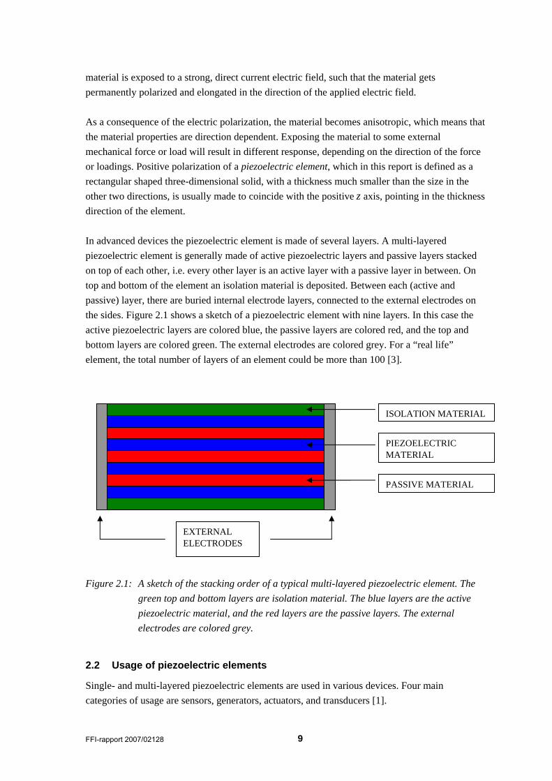
material is exposed to a strong, direct current electric field, such that the material gets permanently polarized and elongated in the direction of the applied electric field. As a consequence of the electric polarization, the material becomes anisotropic, which means that the material properties are direction dependent. Exposing the material to some external mechanical force or load will result in different response, depending on the direction of the force or loadings. Positive polarization of a piezoelectric element, which in this report is defined as a rectangular shaped three-dimensional solid, with a thickness much smaller than the size in the other two directions, is usually made to coincide with the positive z axis, pointing in the thickness direction of the element. In advanced devices the piezoelectric element is made of several layers. A multi-layered piezoelectric element is generally made of active piezoelectric layers and passive layers stacked on top of each other, i.e. every other layer is an active layer with a passive layer in between. On top and bottom of the element an isolation material is deposited. Between each (active and passive) layer, there are buried internal electrode layers, connected to the external electrodes on the sides. Figure 2.1 shows a sketch of a piezoelectric element with nine layers. In this case the active piezoelectric layers are colored blue, the passive layers are colored red, and the top and bottom layers are colored green. The external electrodes are colored grey. For a “real life” element, the total number of layers of an element could be more than 100 [3].
Figure 2.1: A sketch of the stacking order of a typical multi-layered piezoelectric element. The green top and bottom layers are isolation material. The blue layers are the active piezoelectric material, and the red layers are the passive layers. The external electrodes are colored grey.
2.2 Usage of piezoelectric elements
Single- and multi-layered piezoelectric elements are used in various devices. Four main categories of usage are sensors, generators, actuators, and transducers [1].
ISOLATION MATERIAL
PIEZOELECTRIC MATERIAL
PASSIVE MATERIAL
EXTERNAL ELECTRODES
10 FFI-rapport 2007/02128
A sensor typically transforms a force or pressure load to electrical signals, i.e. the piezoelectric effect. Sensors may be divided into two main groups [1]: axial sensors and flexional sensors. For the axial sensors the load or force is applied in the same direction as the direction of polarization of the element. The electric signal is also generated in the same direction. For flexional sensors the applied force is measured in the direction of the polarization, but the force makes the element deform (or bend) in a direction perpendicular to the polarization direction. To generate an electric signal, the pressure or force must be changed. A generator follows the same principle as a sensor. Generators are applied for instance as ignitors in fuel lighters, where it is needed to generate voltages that are sufficient to create a spark across an electrical gap. An actuator transforms an electric signal to mechanical deformation, i.e. the inverse piezoelectric effect. Actuators may be divided into three main groups [1]: axial actuators, transversal actuators, and flexional actuators. An axial actuator accepts an electrical signal in the direction of the polarization of the element, and creates a deformation in the same direction. A transversal actuator also accepts a signal in the direction of polarization, but creates a deformation in the plane perpendicular to this direction. The third actuator type is a bilinear (two-layered) element. The flexional actuator has the same properties as the transversal actuator, but is capable of performing much larger movements. Transducers are applied for converting electrical energy into mechanical vibration energy. Such piezoelectric elements are typically employed in sound and ultrasound devices.
3 Mathematical background In a mathematical setting the mechanical deformation and the electric field distribution are often described by partial differential equations (PDEs), together with boundary and initial conditions. Additional expressions are needed for describing the material and its electric properties, so-called constitutive laws. The PDE (or PDEs), the boundary and initial conditions, and the constitutive law form a complete mathematical description in each case. Piezoelectric materials have both mechanical and electrical properties. Analyses will hence in such cases involve the PDE and the boundary and initial conditions both from the elasticity part and from the electrostatics part. Moreover, the constitutive relations (or laws) involved are extended versions of the relations for each of the two (sub-) problems. The extra terms in the constitutive laws contain the explicit coupling between the material behavior and the electrostatic behavior. In this section we first give a brief introduction to a set of equations and constitutive laws for linear elasticity and linear electrostatics. Then, we show the expressions for the piezoelectric coupling. It should be remarked, that we assume isothermal conditions. This restriction simplifies

FFI-rapport 2007/02128 11
the expressions involved; see e.g. [2] for the expressions obtained when temperature changes are included.
3.1 Electrostatic properties
The Maxwell equations may be used for describing the quasi-static electric field [8;9],
es∇⋅ =D ρ (3.1) and
0∇× =E . (3.2) In (3.1), D is the electric displacement vector, and esρ is a given volume charge density.
However, it may be assumed that there are no free charges within the material; the Gauss’ law requires that the divergence of the electric displacement field is zero [8]. Hence, esρ can be set to
zero. Furthermore, E in (3.2) is the electric field. The relation between the electric field E and the electric potentialφ can be expressed as
φ= −∇E . (3.3)
This latter expression satisfies the constraint in (3.2) exactly [10]. In addition to the governing equations for electrostatics, we need to prescribe some boundary conditions. The essential boundary condition may be expressed as
*φ φ= , (3.4) where φ∗ is a prescribed electric potential on the surface Sφ . Moreover, the natural boundary
condition on the surface Sσ can be expressed
S
i i in D f= , (3.5) where in=n is the outwards normal vector, and S S
if=f is the applied surface charge.
To fully define the mathematical problem, we need to establish a constitutive law. For the electrostatics problem this may be written as
S=D b E , (3.6) where Sb is the permittivity tensor. The other quantities are defined above.

12 FFI-rapport 2007/02128
3.2 Mechanical behavior
The mechanical behavior of a solid continuum may be expressed by the following equilibrium equation [5;8],
b ρ∇⋅ + =σ f u , (3.7) which is based on Newton’s second law. In the above equation the first term on the left hand
side, ij
jxσ∂
∇⋅ =∂
σ , is the divergence of the stress tensor σ , where jx ( 1, 2,3j = ) are the
Cartesian coordinate axes. The second term on the left hand side contains the body forces, e.g. gravity forces ,b b i if bρ= =f , where ρ is the mass density and ib is the component of the body
force in direction i ( 1, 2,3i = ). The term on the right hand side of (3.7) expresses the
acceleration of the solid, where (from the assumption of small displacements) 2
, 2i
i ttuut
∂= =
∂u is
the second derivative of the displacement field [ , , ]u v w=u with respect to time t .
In addition to the above equation, boundary conditions need to be specified. Essential boundary conditions may be defined on part of the surface, uS ,
*
i iu u= , (3.8) where *
iu are prescribed displacements. Moreover, natural boundary conditions may be defined on other parts of the surface, fS ,
S
ij j in qσ = , (3.9) where ijσ is the stress tensor, jn=n is the outwards normal vector to the surface, and S
iq is the
applied surface force. The two surface parts, uS and fS , are non-overlapping.
Because the expression in (3.7) contains time derivatives of second order, we need to define two initial conditions. For instance, we can apply forces that causes an initial deformation of the continuum, that is
0 , 0t= =u u . (3.10) Moreover, we may assume that the displacement field is initially unchanged (in time),
0, 0tt
∂= =
∂u
. (3.11)

FFI-rapport 2007/02128 13
These two initial conditions are used to establish the solution for the first two time steps in a time-stepping scheme, see Section 4.1.3 and [5] for more details. To complete the mathematical formulation, we need to specify the material properties, i.e. the constitutive law. For linear elastic materials the stresses are related to the strains through Hooke’s generalized law, which may be expressed as
ij ijkl klCσ ε= , (3.12) where ijklC is the fourth order elasticity tensor and klε is the strain tensor. For small deformation
cases the strains are expressed by the displacements as follows,
12
jiij
j i
uux x
ε⎛ ⎞∂∂
= +⎜ ⎟⎜ ⎟∂ ∂⎝ ⎠. (3.13)
By utilizing the fact that the stress and the strain tensors are symmetric, and also the symmetry properties of the fourth order elasticity tensor ( ijkl jikl klijC C C= = ), Hooke’s generalized law may
be rewritten using the matrix-vector notation (see Appendix A for more details), =σ Cε , (3.14)
where in this case the stress and strain vectors are expresses as
11
22
33
12
23
31
σσστττ
⎛ ⎞⎜ ⎟⎜ ⎟⎜ ⎟
= ⎜ ⎟⎜ ⎟⎜ ⎟⎜ ⎟⎜ ⎟⎝ ⎠
σ (3.15)
and
11
22
33
12
23
31
εεεγγγ
⎛ ⎞⎜ ⎟⎜ ⎟⎜ ⎟
= ⎜ ⎟⎜ ⎟⎜ ⎟⎜ ⎟⎜ ⎟⎝ ⎠
ε . (3.16)
14 FFI-rapport 2007/02128
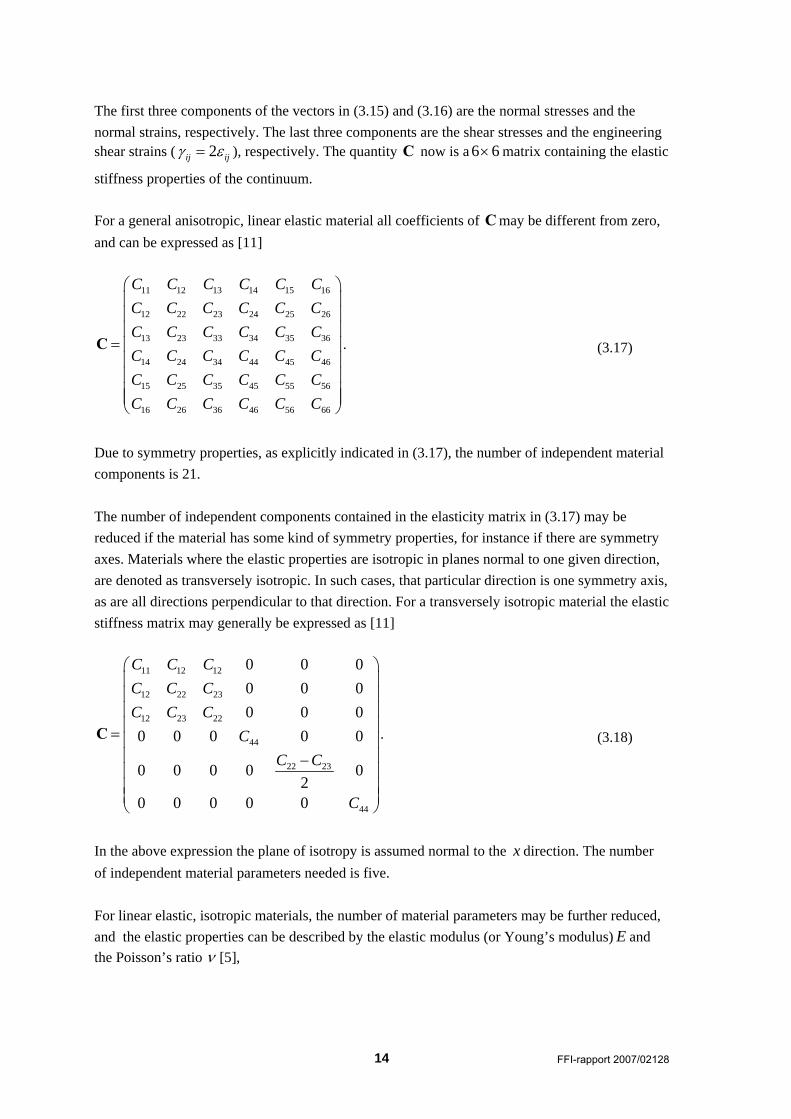
The first three components of the vectors in (3.15) and (3.16) are the normal stresses and the normal strains, respectively. The last three components are the shear stresses and the engineering shear strains ( 2ij ijγ ε= ), respectively. The quantity C now is a 6 6× matrix containing the elastic
stiffness properties of the continuum. For a general anisotropic, linear elastic material all coefficients of C may be different from zero, and can be expressed as [11]
11 12 13 14 15 16
12 22 23 24 25 26
13 23 33 34 35 36
14 24 34 44 45 46
15 25 35 45 55 56
16 26 36 46 56 66
C C C C C CC C C C C CC C C C C CC C C C C CC C C C C CC C C C C C
⎛ ⎞⎜ ⎟⎜ ⎟⎜ ⎟
= ⎜ ⎟⎜ ⎟⎜ ⎟⎜ ⎟⎜ ⎟⎝ ⎠
C . (3.17)
Due to symmetry properties, as explicitly indicated in (3.17), the number of independent material components is 21. The number of independent components contained in the elasticity matrix in (3.17) may be reduced if the material has some kind of symmetry properties, for instance if there are symmetry axes. Materials where the elastic properties are isotropic in planes normal to one given direction, are denoted as transversely isotropic. In such cases, that particular direction is one symmetry axis, as are all directions perpendicular to that direction. For a transversely isotropic material the elastic stiffness matrix may generally be expressed as [11]
11 12 12
12 22 23
12 23 22
44
22 23
44
0 0 00 0 00 0 0
0 0 0 0 0
0 0 0 0 02
0 0 0 0 0
C C CC C CC C C
CC C
C
⎛ ⎞⎜ ⎟⎜ ⎟⎜ ⎟⎜ ⎟= ⎜ ⎟⎜ ⎟−⎜ ⎟⎜ ⎟⎜ ⎟⎝ ⎠
C . (3.18)
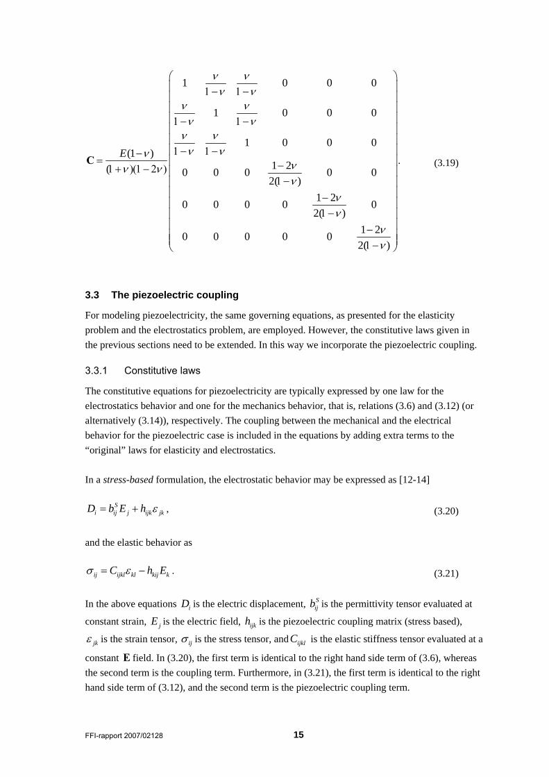
In the above expression the plane of isotropy is assumed normal to the x direction. The number of independent material parameters needed is five. For linear elastic, isotropic materials, the number of material parameters may be further reduced, and the elastic properties can be described by the elastic modulus (or Young’s modulus) E and the Poisson’s ratio ν [5],
FFI-rapport 2007/02128 15
1 0 0 0
1 0 0 0
1 0 0 0(1 )
1 2( 0 0 0 0 02( )
1 20 0 0 0 02( )
1 20 0 0 0 02( )
E
ν νν ν
ν νν ν
ν νν νν
νν νν
νν
νν
⎛ ⎞⎜ ⎟1− 1−⎜ ⎟⎜ ⎟⎜ ⎟1− 1−⎜ ⎟⎜ ⎟⎜ ⎟1− 1−−
= ⎜ ⎟−1+ )(1− 2 ) ⎜ ⎟1−⎜ ⎟
⎜ ⎟−⎜ ⎟1−⎜ ⎟
⎜ ⎟−⎜ ⎟⎜ ⎟1−⎝ ⎠
C . (3.19)
3.3 The piezoelectric coupling
For modeling piezoelectricity, the same governing equations, as presented for the elasticity problem and the electrostatics problem, are employed. However, the constitutive laws given in the previous sections need to be extended. In this way we incorporate the piezoelectric coupling.
3.3.1 Constitutive laws
The constitutive equations for piezoelectricity are typically expressed by one law for the electrostatics behavior and one for the mechanics behavior, that is, relations (3.6) and (3.12) (or alternatively (3.14)), respectively. The coupling between the mechanical and the electrical behavior for the piezoelectric case is included in the equations by adding extra terms to the “original” laws for elasticity and electrostatics. In a stress-based formulation, the electrostatic behavior may be expressed as [12-14]
Si ij j ijk jkD b E h ε= + , (3.20)
and the elastic behavior as
ij ijkl kl kij kC h Eσ ε= − . (3.21) In the above equations iD is the electric displacement, S
ijb is the permittivity tensor evaluated at
constant strain, jE is the electric field, ijkh is the piezoelectric coupling matrix (stress based),
jkε is the strain tensor, ijσ is the stress tensor, and ijklC is the elastic stiffness tensor evaluated at a
constant E field. In (3.20), the first term is identical to the right hand side term of (3.6), whereas the second term is the coupling term. Furthermore, in (3.21), the first term is identical to the right hand side term of (3.12), and the second term is the piezoelectric coupling term.
16 FFI-rapport 2007/02128
Alternatively the constitutive equations may be expressed in a strain-based setting. In this case the electrostatic behavior may be written as (not using indices) [14-17] = +D dσ ξE , (3.22)
and the elastic behavior as = +ε Sσ dE . (3.23)
In this case d is the piezoelectric coupling matrix (strain-based), ξ is the permittivity tensor (strain-based), and S is the mechanical compliance matrix ( 1−=S C ). The other quantities are defined above.
3.3.2 The governing equations and the boundary and initial conditions
Following the derivation and assumptions by Rahman et al. [8] the governing equations for the coupled problem may be expressed as
S lik ikl
i k i k
ub hx x x x
φ ∂∂ ∂ ∂=
∂ ∂ ∂ ∂ (3.24)
and
li ijkl i kij
j k j k
uu C b hx x x x
φρ ρ∂∂ ∂ ∂= + +∂ ∂ ∂ ∂
. (3.25)
The two above equations are obtained from inserting the constitutive laws in (3.20) and (3.21) into (3.1) and (3.7), respectively. In this case, the tensor notation has been applied in the expressions (and not the matrix-vector notation mentioned in Section 3.2). As one can observe, the mechanical deformation iu will affect the electrical behavior (the right hand side of (3.24)), whereas the mechanical behavior is influenced by the electrical potential φ (the last term on the
right hand side of (3.25)). For the (quasi-static) electrostatics problem in (3.24), the essential boundary conditions are expressed in (3.4), whereas the natural boundary conditions may be expressed as in (3.5). It should, however, be remarked that the electric displacement now contains two terms (and not one term, as in the pure electrostatic case). For the elasticity problem in (3.25), the essential boundary conditions are given in (3.8), the natural boundary conditions are given in (3.9), whereas the initial conditions are given in (3.10) and (3.11).
FFI-rapport 2007/02128 17
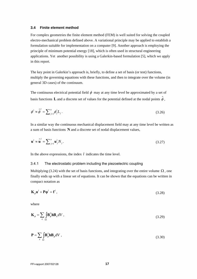
3.4 Finite element method
For complex geometries the finite element method (FEM) is well suited for solving the coupled electro-mechanical problem defined above. A variational principle may be applied to establish a formulation suitable for implementation on a computer [9]. Another approach is employing the principle of minimum potential energy [18], which is often used in structural engineering applications. Yet another possibility is using a Galerkin-based formulation [5], which we apply in this report. The key point in Galerkin’s approach is, briefly, to define a set of basis (or test) functions, multiply the governing equations with these functions, and then to integrate over the volume (in general 3D cases) of the continuum. The continuous electrical potential field φ may at any time level be approximated by a set of
basis functions L and a discrete set of values for the potential defined at the nodal points φ ,
1
l nl lj jjLφ φ φ
=≈ =∑ . (3.26)
In a similar way the continuous mechanical displacement field may at any time level be written as a sum of basis functions N and a discrete set of nodal displacement values,
1
l nl lj jjN
=≈ =∑u u u . (3.27)
In the above expressions, the index l indicates the time level.
3.4.1 The electrostatic problem including the piezoelectric coupling
Multiplying (3.24) with the set of basis functions, and integrating over the entire volume Ω , one finally ends up with a linear set of equations. It can be shown that the equations can be written in compact notation as
l l lφ + =K u Pφ f , (3.28)
where
ue
dVφ φΤ
Ω
=∑∫K B hB , (3.29)
e
dVφ φΤ
Ω
=∑∫P B hB , (3.30)

18 FFI-rapport 2007/02128
and lf is the surface density charge vector. The coefficients of φB and uB contain first
derivatives of the basis functions with respect to the coordinate directions. Assuming that the mechanical displacement field is known, the first term on the left hand side of (3.28) can be moved to the right hand side, and denoted as the load vector l
uf . The linear system
can then be solved for the potential field,
l l lu= −Pφ f f . (3.31)
3.4.2 The elasticity problem including the piezoelectric coupling
Following a similar procedure as in the previous section, the equation of motion may be expressed as [8],
1 1 2 1ˆ2 ( )l l l l l lt+ − −= − + Δ − + +u u u M Ku β Φ , (3.32) where l indicates the current time level, and 1ˆ −M is the inverse of the lumped mass matrix. Moreover,
u ue
dVΤ
Ω
=∑∫K B hB . (3.33)
The vector lβ contains the contributions from the body forces and surface tractions, and lΦ is the
load vector from the electric field. This latter load vector contains the piezoelectric coupling term. Remark that, in static (or quasi-static) cases, only the last term on the right hand side of (3.32) will not vanish. More details about the implementation of the problem on a computer, employing the finite element method, may be found in the following section. For more general FEM theory we refer to [5;18;19].
4 Numerical Modeling A lot of work has been done on modeling piezoelectricity, both when it comes to numerical algorithms and to applications. It is not intended in this report to cover all parts of the research, or to point out any special field of interest. The simulators presented here are implemented as a tool for understanding more about the fundamentals of piezoelectricity. Moreover, the simulators will work as a building block for further research and more advanced applications. For comparison and code verification, simulators are implemented in two different software packages, that is, in Diffpack [5;20] and in MSC.Marc/Mentat [21]. Both simulators are described in the following.

FFI-rapport 2007/02128 19
4.1 Piezoelectric modeling in Diffpack
A simulator for modeling piezoelectricity has been developed in the commercial software package Diffpack [22], which is a C++ based code library well suited for solving ordinary and partial differential equations (ODEs and PDEs, respectively). Developing a simulator in Diffpack gives us the flexibility of defining applications with special features often not supported by other comparable commercial software tools like MSC.Marc, ANSYS and ABAQUS. In addition we have full control of program details, solution techniques, and the numerical algorithm employed. In other software tools, most of these things are hidden inside a “black box”. On the other hand, in Diffpack we need to do more low-level programming, which is often more time consuming and error prone. However, employing already implemented standard simulators in Diffpack, and extending these for our special application case, the time needed and the number of bugs introduced will decrease.
4.1.1 The class hierarchy of the Diffpack simulator
The Diffpack simulator for simulating piezoelectricity is based on two standard and already implemented simulators in Diffpack; one simulator for modeling linear elasticity and one simulator applicable for solving the electrostatics problem (i.e. a simulator for solving the Poisson’s equation). Some modifications are needed in the current solvers for including the piezoelectric coupling. In addition, we need a manager class for connecting the two involved (sub-) simulators. The class structure for the piezoelectricity solver is shown in Figure 4.1. Here, Poisson2 is the standard time-dependent Poisson solver already found in Diffpack. Moreover, PoissonPiezo1 is a new class taking into account the contribution to the electrostatics part from the mechanical deformation, i.e. the piezoelectric coupling. Furthermore, Elasticity2 is the standard Diffpack solver for isotropic, linear elastic problems, applying the engineering approach (i.e. the matrix-vector notation). Elasticity3 is a new class including linear elastic, anisotropic materials. Also, ElasticVib1 is a standard Diffpack solver for time-dependent elastic motion, where some modifications are made to the original solver. These latter code adjustments are due to the inclusion of Elasticity3. Moreover, ElasticVibPiezo1 is a new class that takes into account the contribution from the electric field, i.e. the piezoelectric coupling. Finally, PiezoElec1 is a new class for managing the solve process of the piezoelectric problem. This latter class is in Diffpack terminology often referred to as the “manager class” [5].
4.1.2 The finite element method
When writing a computer program in Diffpack/C++, some low-level programming details are required. In this section we give the expressions required, namely the (problem-dependent) expressions needed in the integrands (volume integral) and integrands4side (surface integral) functions. These functions are common in most Diffpack simulators, and must be implemented for each simulator. More details about Diffpack simulators are found in [5].

20 FFI-rapport 2007/02128
Figure 4.1: Class structure in Diffpack for the piezoelectricity simulator. The classes Poisson2, Elasticity2, and ElasticVib1 are standard solvers. The classes PoissonPiezo1, Elasticity3, ElasticVibPiezo1, and PiezoElec1 are developed for the piezoelectric coupling application.
.
4.1.2.1 The electrostatics problem with piezoelectric coupling
For the electrostatics problem including piezoelectricity it is appropriate to start with the equation in (3.24). We write out all terms, multiply with the basis functions, and integrate over the domain of the continuum. For the left hand side of (3.24), applying Green’s theorem for integration by parts, and without doing any assumptions of the components of the permittivity tensor, we get that,
ElasticVibPiezo1 PoissonPiezo1
PiezoElec1
ElasticVib1 Possion2
Elasticity3
Elasticity2
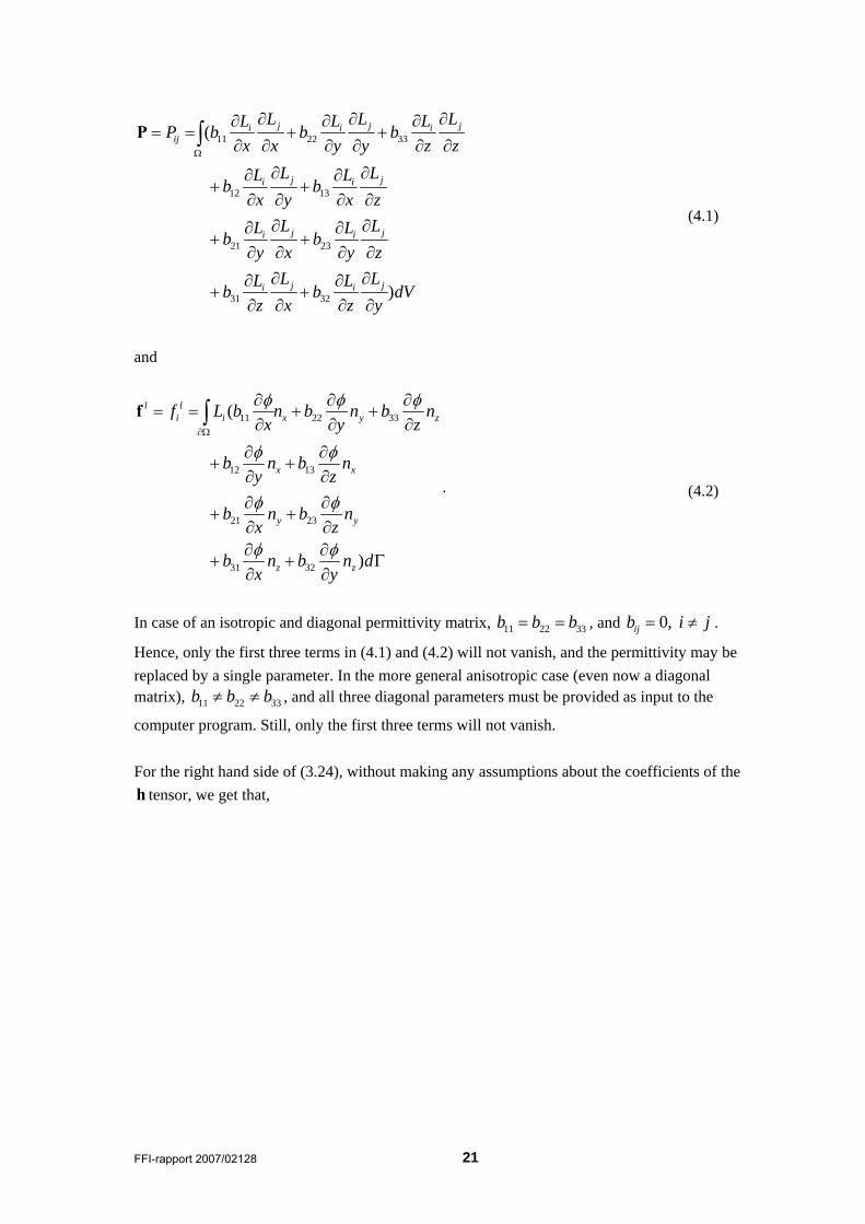
FFI-rapport 2007/02128 21
11 22 33
12 13
21 23
31 32
(
)
j j ji i iij
j ji i
j ji i
j ji i
L L LL L LP b b bx x y y z z
L LL Lb bx y x z
L LL Lb by x y z
L LL Lb b dVz x z y
Ω
∂ ∂ ∂∂ ∂ ∂= = + +
∂ ∂ ∂ ∂ ∂ ∂
∂ ∂∂ ∂+ +
∂ ∂ ∂ ∂∂ ∂∂ ∂
+ +∂ ∂ ∂ ∂
∂ ∂∂ ∂+ +
∂ ∂ ∂ ∂
∫P
(4.1)
and
11 22 33
12 13
21 23
31 32
(
)
l li i x y z
x x
y y
z z
f L b n b n b nx y z
b n b ny z
b n b nx z
b n b n dx y
φ φ φ
φ φ
φ φ
φ φ
∂Ω
∂ ∂ ∂= = + +
∂ ∂ ∂
∂ ∂+ +
∂ ∂∂ ∂
+ +∂ ∂∂ ∂
+ + Γ∂ ∂
∫f
. (4.2)
In case of an isotropic and diagonal permittivity matrix, 11 22 33b b b= = , and 0, ijb i j= ≠ .
Hence, only the first three terms in (4.1) and (4.2) will not vanish, and the permittivity may be replaced by a single parameter. In the more general anisotropic case (even now a diagonal matrix), 11 22 33b b b≠ ≠ , and all three diagonal parameters must be provided as input to the
computer program. Still, only the first three terms will not vanish. For the right hand side of (3.24), without making any assumptions about the coefficients of the h tensor, we get that,
22 FFI-rapport 2007/02128
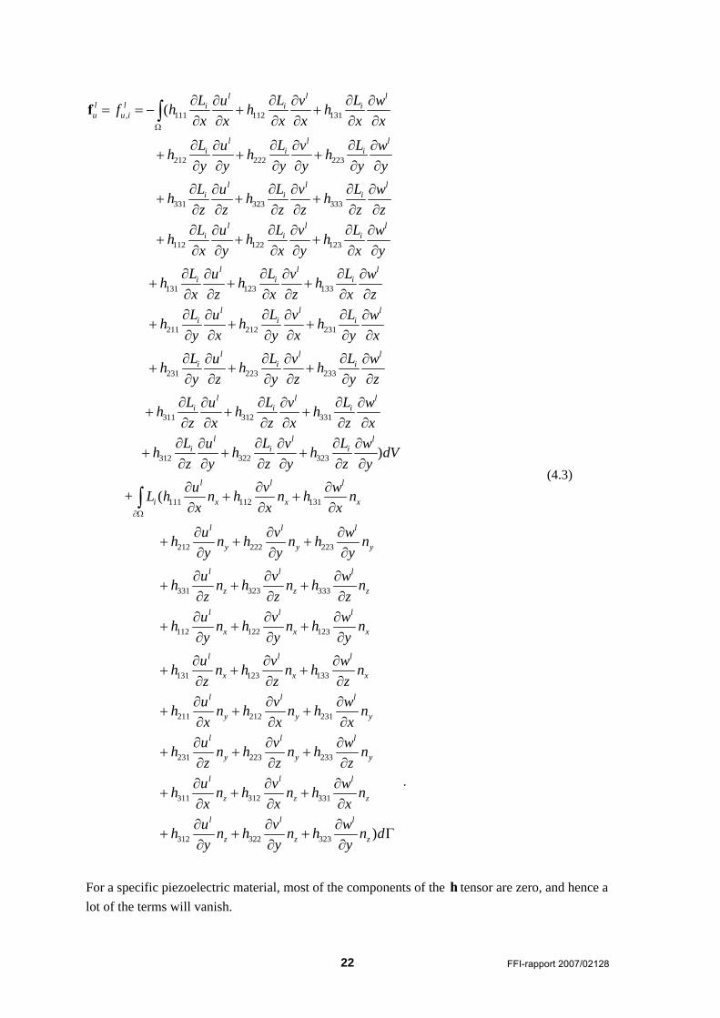
, 111 112 131
212 222 223
331 323 333
(
l l ll l i i iu u i
l l li i i
l l li i i
L L Lu v wf h h hx x x x x x
L L Lu v wh h hy y y y y yL L Lu v wh h hz z z z z z
Ω
∂ ∂ ∂∂ ∂ ∂= = − + +
∂ ∂ ∂ ∂ ∂ ∂
∂ ∂ ∂∂ ∂ ∂+ + +
∂ ∂ ∂ ∂ ∂ ∂
∂ ∂ ∂∂ ∂ ∂+ + +
∂ ∂ ∂ ∂ ∂ ∂
∫f
112 122 123
131 123 133
211 212 231
231
l l li i i
l l li i i
l l li i i
li
L L Lu v wh h hx y x y x y
L L Lu v wh h hx z x z x zL L Lu v wh h hy x y x y xL uhy z
∂ ∂ ∂∂ ∂ ∂+ + +
∂ ∂ ∂ ∂ ∂ ∂
∂ ∂ ∂∂ ∂ ∂+ + +
∂ ∂ ∂ ∂ ∂ ∂∂ ∂ ∂∂ ∂ ∂
+ + +∂ ∂ ∂ ∂ ∂ ∂
∂ ∂+
∂ ∂ 223 233
311 312 331
312 322 323
111 112 131
)
+ (
l li i
l l li i i
l l li i i
l l l
i x x
L Lv wh hy z y z
L L Lu v wh h hz x z x z x
L L Lu v wh h h dVz y z y z yu v wL h n h n hx x∂Ω
∂ ∂∂ ∂+ +
∂ ∂ ∂ ∂
∂ ∂ ∂∂ ∂ ∂+ + +
∂ ∂ ∂ ∂ ∂ ∂∂ ∂ ∂∂ ∂ ∂
+ + +∂ ∂ ∂ ∂ ∂ ∂
∂ ∂ ∂+ +
∂ ∂∫
212 222 223
331 323 333
112 122 123
131
x
l l l
y y y
l l l
z z z
l l l
x x x
l
x
nx
u v wh n h n h ny y yu v wh n h n h nz z zu v wh n h n h ny y yuh nz
∂
∂ ∂ ∂+ + +
∂ ∂ ∂
∂ ∂ ∂+ + +
∂ ∂ ∂∂ ∂ ∂
+ + +∂ ∂ ∂
∂+
∂ 123 133
211 212 231
231 223 233
311 312 331
l l
x x
l l l
y y y
l l l
y y y
l l l
z z z
v wh n h nz z
u v wh n h n h nx x xu v wh n h n h nz z zu v wh n h n h nx x x
∂ ∂+ +
∂ ∂∂ ∂ ∂
+ + +∂ ∂ ∂∂ ∂ ∂
+ + +∂ ∂ ∂∂ ∂ ∂
+ + +∂ ∂ ∂
312 322 323 )l l l
z z zu v wh n h n h n dy y y
∂ ∂ ∂+ + + Γ
∂ ∂ ∂
.
(4.3)
For a specific piezoelectric material, most of the components of the h tensor are zero, and hence a lot of the terms will vanish.

FFI-rapport 2007/02128 23
This completes the (detailed) description of the terms in (3.31). The above volume and surface integral expressions are implemented into the integrands and integrands4side functions, respectively, of class PoissonPiezo1.
4.1.2.2 The elasticity problem with piezoelectric coupling
For the elasticity problem, applying the matrix-vector notation, we end up with the following expression, similar to the form in (3.32) [5;8],
1 1 2 2 22ll l l T l
j j j i i it dV t N dV t N dρ− +
Ω Ω ∂Ω
− + + Δ = Δ + Δ Γ∫ ∫ ∫Mu Mu Mu B σ b t , (4.4)
where
i jN N dVρΩ
= ∫M (4.5)
is the mass matrix. In the computer code a lumped mass matrix is applied. In this way the mass matrix becomes invertible, and (4.4) may be solved for the unknown displacement vector field at the next time step 1l
j+u .
In (4.4), the contribution from the electric field is contained in the fourth term on the left hand side and in the second term on the right hand side. The fourth term on the left hand side, inserting the constitutive law on matrix-vector form (see Appendix A for details) becomes
( )l lT T T l T l T T l
i i i j j idV dV dV dVΩ Ω Ω Ω
= − = −∫ ∫ ∫ ∫B σ B Cε h E B CB u B h E . (4.6)
In the above expression the first term is the “standard” stiffness matrix for linear elastic problems. The only new code implementation needed for this part is the specification of anisotropic material properties. The second term is the part dealing with the piezoelectric coupling, and hence, we focus on this latter term here. The second term may be written as
T T l T li i EdV dV
Ω Ω
=∫ ∫B h E B σ , (4.7)
where
,11 111 1 211 2 311 3
,22 122 1 222 2 322 3
,33 133 1 233 2 333 3
,12 112 1 212 2 312 3
,23 123 1 223 2 323 3
,31 131 1 231 2 331 3
l l l lEl l l lEl l l lEl
E l l l lEl l l lEl l l lE
h E h E h Eh E h E h Eh E h E h Eh E h E h Eh E h E h Eh E h E h E
σσσσσσ
⎛ ⎞ ⎛ + +⎜ ⎟
+ +⎜ ⎟⎜ ⎟ + +
= =⎜ ⎟+ +⎜ ⎟
⎜ ⎟ + +⎜ ⎟⎜ ⎟ + +⎝ ⎠
σ
⎞⎜ ⎟⎜ ⎟⎜ ⎟⎜ ⎟⎜ ⎟⎜ ⎟⎜ ⎟⎜ ⎟⎝ ⎠
, (4.8)
24 FFI-rapport 2007/02128
from which we may write
, ,11 , ,12 , ,31
, ,22 , ,12 , ,23
, ,33 , ,23 , ,31
l l li x E i y E i z E
T T l l l li i y E i x E i z E
l l li z E i y E i x E
N N N dV
dV N N N dV
N N N dV
σ σ σ
σ σ σ
σ σ σ
Ω
Ω Ω
Ω
⎛ ⎞+ +⎜ ⎟
⎜ ⎟⎜ ⎟= + +⎜ ⎟⎜ ⎟⎜ ⎟+ +⎜ ⎟⎝ ⎠
∫
∫ ∫
∫
B h E , (4.9)
with ,i
i xNNx
∂=
∂, ,
ii y
NNy
∂=∂
, and ,i
i zNNz
∂=
∂.
In a similar way, the second term on the right hand side of (4.4) may be written,
l l li M i E iN d N d N d
∂Ω ∂Ω ∂Ω
Γ = Γ − Γ∫ ∫ ∫t t t . (4.10)
In the above expression, the first term is the “standard” boundary term, whereas the second term is the natural boundary condition from the piezoelectric coupling. Again, we focus on the piezoelectric coupling part. Having that , ,
l l lE E r E rs st nσ= =t , where ,
l lE rs prs ph Eσ = , and where
[ , , ]Ts x y zn n n n= =n is the normal vector, the latter term of (4.10) may be written,
, , 2 , 3
,2 ,22 ,23
,3 ,32 ,33
( )
( )
( )
l l li E x E y E z
l l l lE i i E x E y E z
l l li E x E y E z
N n n n d
N d N n n n d
N n n n d
σ σ σ
σ σ σ
σ σ σ
11 1 1∂Ω
1∂Ω ∂Ω
1∂Ω
⎛ ⎞+ + Γ⎜ ⎟
⎜ ⎟⎜ ⎟Γ = + + Γ⎜ ⎟⎜ ⎟⎜ ⎟+ + Γ⎜ ⎟⎝ ⎠
∫
∫ ∫
∫
t . (4.11)
Most of the terms in the piezoelectric coupling matrix often vanish. This will simplify the final expressions. This completes the (detailed) description of (4.4). The above volume and surface integral expressions are implemented into the integrands and integrands4side functions, respectively, of class ElasticVibPiezo1.
4.1.3 Solution algorithm
Rahman et al. [8] have applied a solution algorithm involving two sub-solvers; one sub-solver for the elasticity part, and one sub-solver for the electrostatics part. A similar solution algorithm is presented by Gaudenzi and Bathe [9]. In their approaches, for each time level the two sub-
FFI-rapport 2007/02128 25
problems are solved sequentially. Iterations are performed at each time level, always applying the latest solution fields in the computations. The procedure is repeated until a certain error tolerance is fulfilled. Employing sub-solvers, one is able to reuse already existing simulators, and need only to add the problem specific part for the particular application. Generally, this is a fundamental approach in object-oriented programming, which also will be adopted in our case. Assuming now that proper initial conditions are established for the elasticity problem, the main algorithm can be written as follows:
1. Solve with initial values to obtain initial conditions for 0φ and 0u 2. Compute the error e 3. While crite e> , repeat steps 1 and 2
4. Update field values; 1 0=φ φ and 1 0=u u
5. Solve the elasticity problem, including the piezoelectric coupling 6. Solve the electrostatic problem, including the piezoelectric coupling 7. Compute the error 8. While crite e> , repeat steps 5-7
In static problems, the computation of initial values is not needed. In this case, the solution algorithm starts at step 5. Also remark, that in the above solution algorithm the elasticity problem is solved first. The updated solution field (i.e. the displacement field) is then applied in the electrostatics solve. This solution order is typically applied for simulating the direct piezoelectric effect, where an externally applied pressure load, or force, results in generation of electricity. For simulating the inverse piezoelectric effect, i.e. the exposure of an electric potential resulting in a mechanical deformation, steps 5 and 6 must be switched. In this case the electrostatic sub-problem is solved first. Then the updated solution field values are applied in the solve process for the elasticity sub-problem. As an alternative to establishing two sub-problems and solving the piezoelectricity problem in an iterative way, the entire problem can be solved fully coupled as one linear system. We do not go any further into describing this approach in this report.
4.2 Piezoelectric modeling in MSC.Marc
A simulator is also implemented in MSC.Marc [23], which is a finite element (FE) solver that supports modeling of piezoelectricity. MSC.Marc is in this case used in combination with Mentat. Mentat is the graphical user interface (GUI) for the MSC.Marc FE solver. The GUI is very convenient for the pre and post processing part of the analysis. In this case all code development is more high-level, and hence also less time consuming. The user only needs to provide the input data. Advanced and well tested solvers are already contained in the software package, and we do not need to define any algorithm for the solution process

26 FFI-rapport 2007/02128
ourselves. On the other side, most programming details are hidden “behind the curtains”. Incorrect use of the software may give wrong answers, although the results appear to be reasonable. For modeling piezoelectricity in MSC.Marc we need to establish a problem description, which is saved on a file. The problem description file may later be opened and modified. The problem description, including geometry and element discretization, material properties, boundary conditions, element type, and solution process options, can be specified in Mentat. Alternatively, one may employ the PyMentat module [24]. All input data and other specifications are then written in a Python script file, which can be loaded into Mentat. In this way only one file needs to be saved. Moreover, all commands and chosen options (besides the default options set by the program) are explicitly given in the Python script. This latter approach may speed up the time spent and effort put into the debugging process.
5 Test cases In this section we show some numerical results from running the same problem in Diffpack and MSC.Marc. Although the simulators presented above are capable of handling time-dependent problems, we restrict our examples to static simulations. First, at time of writing static simulations are immediately needed in the project work, and hence more relevant than dynamic simulations. Furthermore, the primary aim in this report is to verify the code implementation, both the self-developed Diffpack solver and the MSC.Marc solver. Finally, we try to get a better understanding of the fundamental aspects of the problem itself. For these purposes it is appropriate to keep the examples relatively simple and time-independent. Obtaining the same numerical results in two independent software tools, one may conclude that the implementations are correct. Solving the same problem employing different software tools may in some cases produce slightly different results. Such differences may be due to the choice of solution method, accuracy tolerances, integration rules, employment of different computers and so on. In this case the Diffpack simulator and the MSC.Marc simulator are run on different computers, due to the fact that the software tools are installed on different computers. Moreover, for the MSC.Marc solver, a lot of computational details are hidden. Because of the above mentioned aspects, we only show (and compare) the primary solution fields for most of the cases included in this report. More data is, however, available for further analysis. In all test cases we consider a rectangular shaped test specimen, with width and length5 mm and thickness 0.1995 mm , where z is the global thickness direction, and the other two global axes are defined according to the right hand rule. The thickness value is a consequence of using the grid generation tools in MSC.Marc. Moreover, the specimen is assumed to be made of pure piezoelectric material, which often is referred to as a single-layered piezoelectric element (see Section 2.1). For all cases the test specimen is discretized using 10 10 15× × elements. Corresponding element types (i.e. same number of nodes and order of the basis functions) are

FFI-rapport 2007/02128 27
applied in the simulators. A sketch of the geometry of the specimen, with the element mesh, is shown in Figure 5.1.
Figure 5.1: Geometry and element mesh of the test specimen. The size of the specimen is 5 5 1.995 mm× × , with 10 10 15× × elements.
Color plots of the primary unknowns are shown for each test case. Remark that the color scales are different for the Diffpack and the MSC.Marc results; the software tools applied for plotting have predefined color scaling. In addition, we give the values at a set of nodal points. Table 5.1 lists the nodal point coordinates. Each geometric location has been given a point identification number.
Table 5.1: Coordinates, with point identification number, for the seven nodal points, where the primary field values are given.
Point id X Y Z P1 0.0 0.0025 0.001064P2 0.0025 0.0025 0.001064P3 0.005 0.0025 0.001064P4 0.0025 0.0 0.001064P5 0.0025 0.005 0.001064P6 0.005 0.0025 0.0 P7 0.0025 0.0025 0.001995
28 FFI-rapport 2007/02128
We start with a pure elasticity problem, including both an isotropic and a transversely isotropic material case. Then, we continue with a test case for a pure electrostatics problem. In this second case the permittivity is first set equal in all coordinate directions (i.e. isotropic permittivity), and then different in the thickness direction compared to the in-plane directions (i.e. orthotropic permittivity). Finally, we run two different piezoelectricity test cases, that is, a sensor/generator case (direct piezoelectric effect) and an actuator case (inverse piezoelectric effect). For the piezoelectricity test cases, anisotropic properties are chosen for both the elasticity part and the electrostatics part.
5.1 Elastic test specimen
In this first test case we consider a pure elasticity problem. The test specimen is in this case restricted from movement at 0.0z = . At 1.995 mmz = a pressure load 250000 N/mp = is
applied (pointing in the negative z direction). Two different linear elastic materials, both with mass density 37750 kg/mρ = , are investigated.
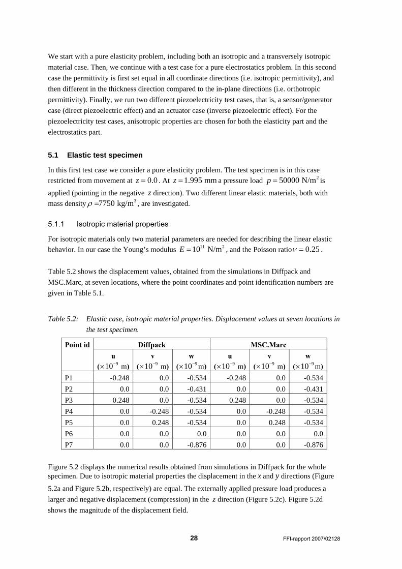
5.1.1 Isotropic material properties
For isotropic materials only two material parameters are needed for describing the linear elastic behavior. In our case the Young’s modulus 11 210 N/mE = , and the Poisson ratio 0.25ν = . Table 5.2 shows the displacement values, obtained from the simulations in Diffpack and MSC.Marc, at seven locations, where the point coordinates and point identification numbers are given in Table 5.1.
Table 5.2: Elastic case, isotropic material properties. Displacement values at seven locations in the test specimen.
Diffpack MSC.Marc Point id u
( 910−× m) v
( 910−× m)w
( 910−× m)u
( 910−× m)v
( 910−× m) w
( 910−× m) P1 -0.248 0.0 -0.534 -0.248 0.0 -0.534 P2 0.0 0.0 -0.431 0.0 0.0 -0.431 P3 0.248 0.0 -0.534 0.248 0.0 -0.534 P4 0.0 -0.248 -0.534 0.0 -0.248 -0.534 P5 0.0 0.248 -0.534 0.0 0.248 -0.534 P6 0.0 0.0 0.0 0.0 0.0 0.0 P7 0.0 0.0 -0.876 0.0 0.0 -0.876
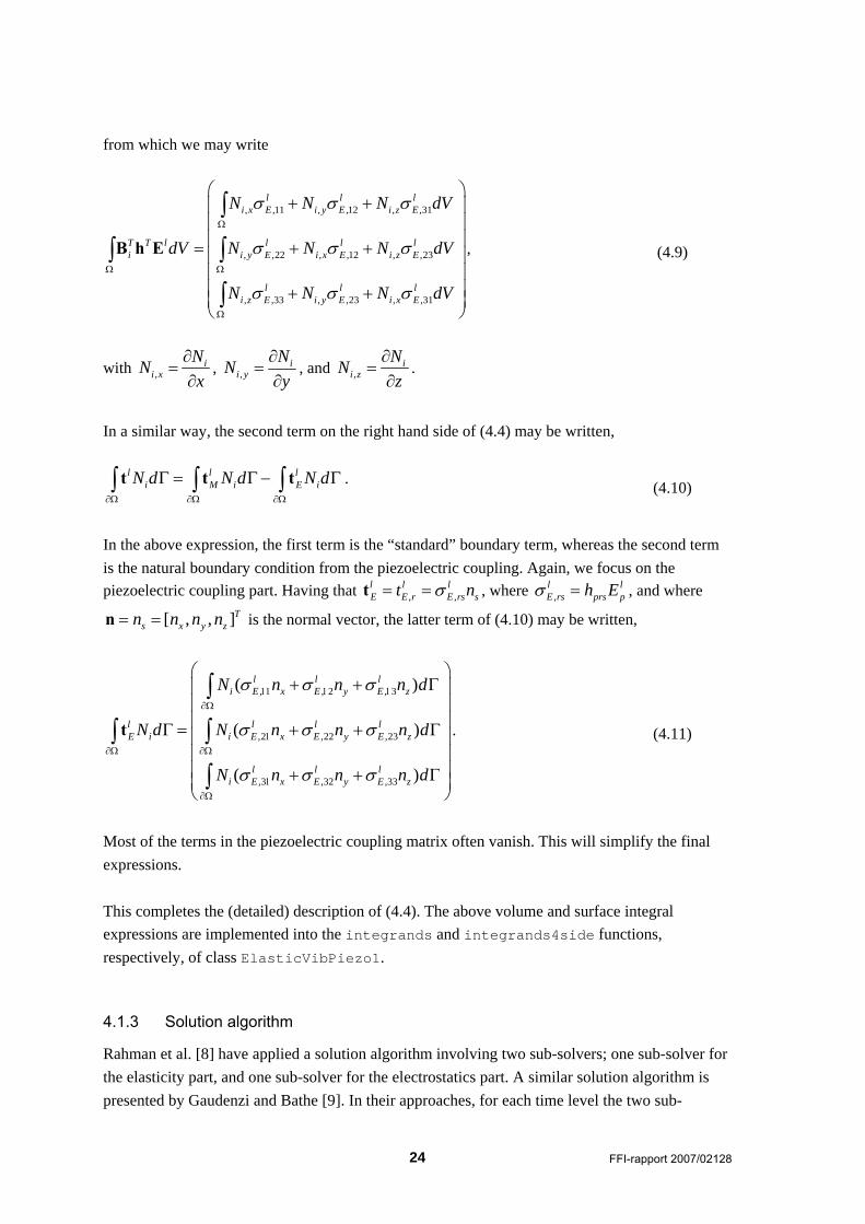
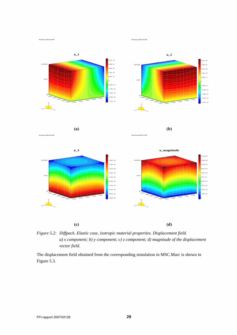
Figure 5.2 displays the numerical results obtained from simulations in Diffpack for the whole specimen. Due to isotropic material properties the displacement in the x and y directions (Figure
5.2a and Figure 5.2b, respectively) are equal. The externally applied pressure load produces a larger and negative displacement (compression) in the z direction (Figure 5.2c). Figure 5.2d shows the magnitude of the displacement field.
FFI-rapport 2007/02128 29
Wed Aug 8 08:55:05 2007
u_1
−3.23e−10
−2.58e−10
−1.94e−10
−1.29e−10
−6.46e−11
0
6.46e−11
1.29e−10
1.94e−10
2.58e−10
3.23e−10
XY
Z
0
0.001
0.001995
00.001
0.0020.003
0.0040.005
00.001
0.0020.003
0.0040.005
Wed Aug 8 08:55:29 2007
u_2
−3.23e−10
−2.58e−10
−1.94e−10
−1.29e−10
−6.46e−11
0
6.46e−11
1.29e−10
1.94e−10
2.58e−10
3.23e−10
XY
Z
0
0.001
0.001995
00.001
0.0020.003
0.0040.005
00.001
0.0020.003
0.0040.005
(a) (b) Wed Aug 8 08:55:56 2007
u_3
−1.09e−09
−9.81e−10
−8.72e−10
−7.63e−10
−6.54e−10
−5.45e−10
−4.36e−10
−3.27e−10
−2.18e−10
−1.09e−10
0
XY
Z
0
0.001
0.001995
00.001
0.0020.003
0.0040.005
00.001
0.0020.003
0.0040.005
Wed Aug 8 08:56:27 2007
u_magnitude
0
1.18e−10
2.36e−10
3.54e−10
4.72e−10
5.9e−10
7.07e−10
8.25e−10
9.43e−10
1.06e−09
1.18e−09
XY
Z
0
0.001
0.001995
00.001
0.0020.003
0.0040.005
00.001
0.0020.003
0.0040.005
(c) (d)
Figure 5.2: Diffpack. Elastic case, isotropic material properties. Displacement field. a) x component; b) y component; c) z component; d) magnitude of the displacement vector field.
The displacement field obtained from the corresponding simulation in MSC.Marc is shown in Figure 5.3.
30 FFI-rapport 2007/02128
(a) (b)
(c) (d)
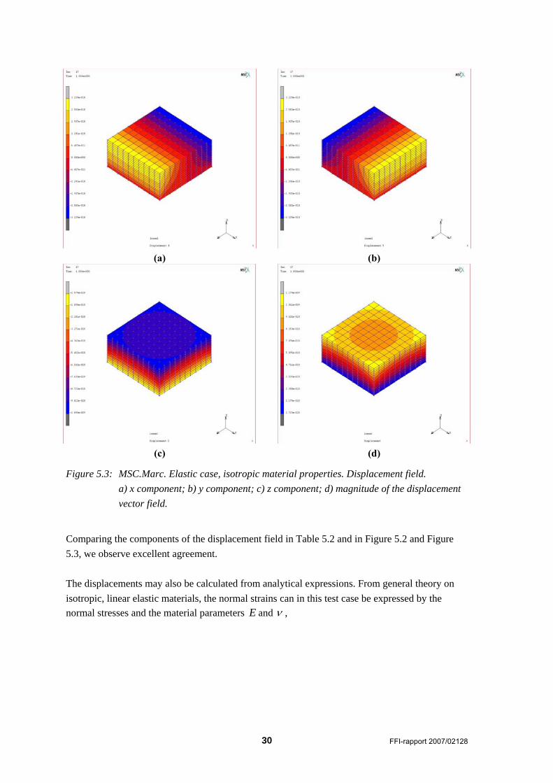
Figure 5.3: MSC.Marc. Elastic case, isotropic material properties. Displacement field. a) x component; b) y component; c) z component; d) magnitude of the displacement vector field.
Comparing the components of the displacement field in Table 5.2 and in Figure 5.2 and Figure 5.3, we observe excellent agreement. The displacements may also be calculated from analytical expressions. From general theory on isotropic, linear elastic materials, the normal strains can in this test case be expressed by the normal stresses and the material parameters E and ν ,
FFI-rapport 2007/02128 31
(1 )
(1 )
2
yx xz zx
y x xz zy
yx xz zz
σσ σσ σε ν ν ν ν
σ σ σσ σε ν ν ν ν
σσ σσ σε ν ν ν
= − − = − −Ε Ε Ε Ε Ε
= − − = − −Ε Ε Ε Ε Ε
= − − = −Ε Ε Ε Ε Ε
. (5.1)
In the above expressions we have used that the normal stresses, xσ and yσ , in this case are equal,
but different from zσ . Moreover, a large pressure load is applied to the top surface, whereas the
bottom surface is restricted from movement in all directions. The remaining four sides are
unloaded and free to move. From this we can conclude that the quantity x
Eσ
in the expressions in
(5.1) typically is much smaller than z pE Eσ
= − , and hence may be neglected. Hence, we may
write,
0
0
0
x
y
z
u pu
v pvw p
w
ε ν
ε ν
ε
Δ= =
ΕΔ
= =Ε
Δ= = −
Ε
, (5.2)
where uΔ is the displacement and 0u is the original length of the specimen in the global
x direction; analogous for the two other directions. Inserting material parameters and lengths of the undeformed test specimen, we get
10011
10011
0.25 0.005 50000 m 6.25 10 m10
0.001995 50000 m 9.975 10 m10
u pu v
w pw
ν −
−
× ×Δ = Δ = = = ×
Ε×
Δ = − = − = − ×Ε
. (5.3)
The analytic displacement in the z direction is close to the displacement value in the center node on the top surface (location P7 in Table 5.2). Moreover, at the top surface the analytic displacement values in the other directions are also very close to the numerical values (Figure 5.2a and b, and Figure 5.3a and b). Applying the expressions in (5.1) and running a test case where the bottom surface is allowed to move in the x and y directions, would probably result in
better agreement between the numerical and analytical values.
5.1.2 Transversely isotropic material properties
In this second case the material properties of the test specimen are transversely isotropic. Piezoelectric materials, which are central in this study, typically have transversely isotropic

32 FFI-rapport 2007/02128
material properties (for example man-made ceramics) or anisotropic material properties (for example quartz). In our case the elasticity matrix is given by
11 2
1.2035 0.7518 0.7509 0 0 00.7518 1.2035 0.7509 0 0 00.7509 0.7509 1.1087 0 0 0
10 N/m0 0 0 0.2257 0 00 0 0 0 0.2105 00 0 0 0 0 0.2105
⎛ ⎞⎜ ⎟⎜ ⎟⎜ ⎟
= ×⎜ ⎟⎜ ⎟⎜ ⎟⎜ ⎟⎜ ⎟⎝ ⎠
C , (5.4)
where the material is isotropic in planes normal to the z direction. Table 5.3 gives the displacement values obtained in Diffpack and MSC.Marc at the same seven locations as in the isotropic material case.
Table 5.3: Elastic case, anisotropic material properties. Displacement values at seven locations in the test specimen.
Diffpack MSC.Marc Point id u
( 910−× m) v
( 910−× m)w
( 910−× m)u
( 910−× m)v
( 910−× m)w
( 910−× m) P1 -0.749 0.0 -0.892 -0.749 0.0 -0.892 P2 0.0 0.0 -0.581 0.0 0.0 -0.581 P3 0.749 0.0 -0.892 0.749 0.0 -0.892 P4 0.0 -0.749 -0.892 0.0 -0.749 -0.892 P5 0.0 0.749 -0.892 0.0 0.749 -0.892 P6 0.0 0.0 0.0 0.0 0.0 0.0 P7 0.0 0.0 -1.379 0.0 0.0 -1.379
Figure 5.4 and Figure 5.5 show the components and the magnitude of the displacement field in this case. With isotropic material properties in planes normal to the z direction, the displacement components in the x and y directions become equal. Moreover, the agreement between the
numerical results in Diffpack and MSC.Marc are excellent also in this case.

FFI-rapport 2007/02128 33
Wed Aug 8 09:43:04 2007
u_1
−9.56e−10
−7.65e−10
−5.74e−10
−3.83e−10
−1.91e−10
0
1.91e−10
3.83e−10
5.74e−10
7.65e−10
9.56e−10
XY
Z
0
0.001
0.001995
00.001
0.0020.003
0.0040.005
00.001
0.0020.003
0.0040.005
Wed Aug 8 09:43:15 2007
u_2
−9.56e−10
−7.65e−10
−5.74e−10
−3.83e−10
−1.91e−10
0
1.91e−10
3.83e−10
5.74e−10
7.65e−10
9.56e−10
XY
Z
0
0.001
0.001995
00.001
0.0020.003
0.0040.005
00.001
0.0020.003
0.0040.005
(a) (b) Wed Aug 8 09:43:29 2007
u_3
−2.04e−09
−1.84e−09
−1.63e−09
−1.43e−09
−1.22e−09
−1.02e−09
−8.17e−10
−6.12e−10
−4.08e−10
−2.04e−10
0
XY
Z
0
0.001
0.001995
00.001
0.0020.003
0.0040.005
00.001
0.0020.003
0.0040.005
Wed Aug 8 09:43:44 2007
u_magnitude
0
2.44e−10
4.87e−10
7.31e−10
9.75e−10
1.22e−09
1.46e−09
1.71e−09
1.95e−09
2.19e−09
2.44e−09
XY
Z
0
0.001
0.001995
00.001
0.0020.003
0.0040.005
00.001
0.0020.003
0.0040.005
(c) (d)
Figure 5.4: Diffpack .Elastic case, anisotropic material properties. Displacement field. a) x component; b) y component; c) z component; d) magnitude of the displacement vector field.

34 FFI-rapport 2007/02128
(a) (b)
(c) (d)
Figure 5.5: MSC.Marc. Elastic case, anisotropic material properties. Displacement field. a) x component; b) y component; c) z component; d) magnitude of the displacement vector field.
5.2 Electrostatic test specimen
In this next case we consider a pure electrostatics problem. At 0.0 mmz = the electric potential is set equal to zero, whereas at 1.995 mmz = the potential value is 10000 V . The electric field can be expressed as the negative gradient of the electric potential, see (3.3). In this case the potential in the z direction is the most important and interesting component. With the chosen potential value and test specimen thickness, the third component of the electric field becomes
63
10000 V/m 5.01 10 V/m0.001995
E = − = − × . (5.5)
FFI-rapport 2007/02128 35
Piezoelectric materials typically have anisotropic permittivity properties. We now investigate how, and if, the permittivity will influence on the distribution of the electric potential and the electric field.
5.2.1 Isotropic permittivity
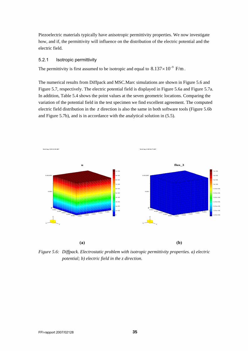
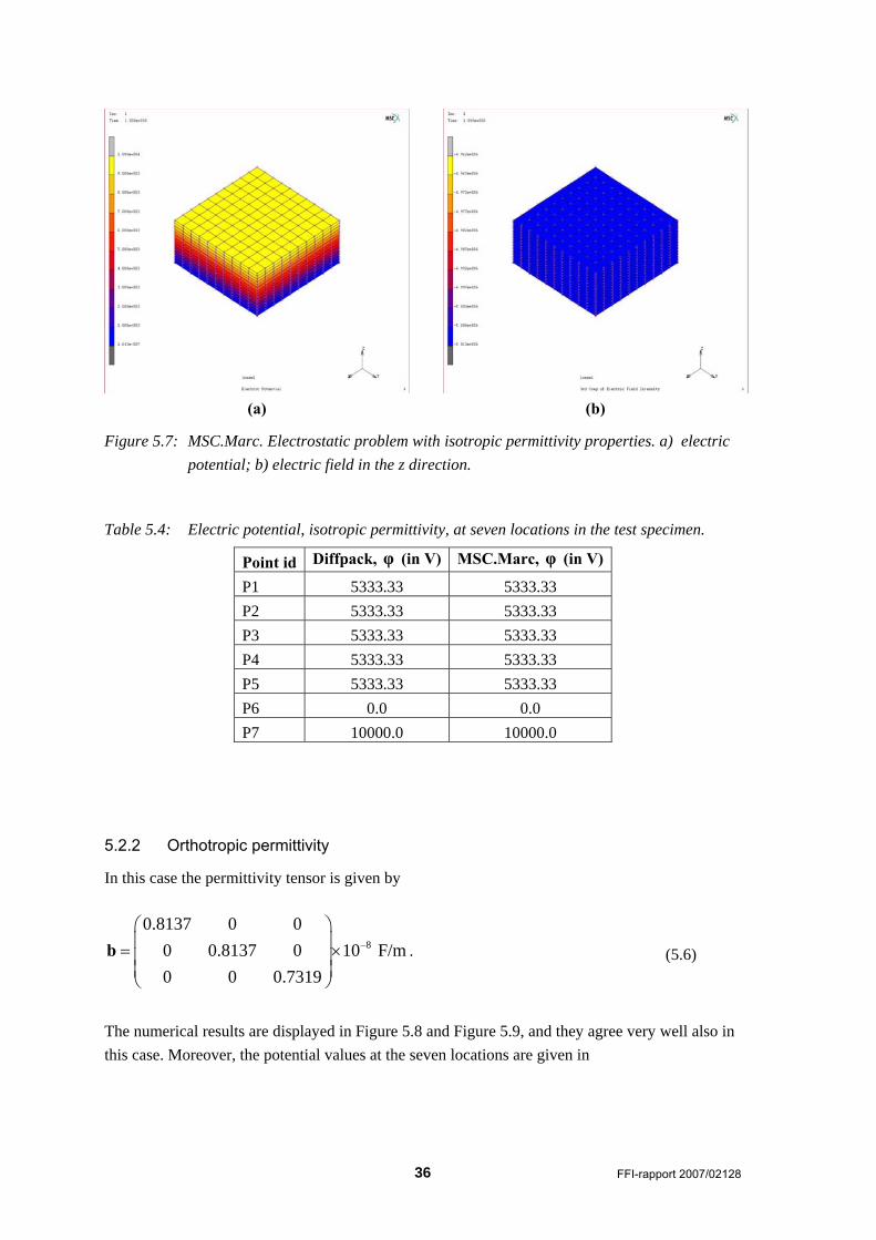
The permittivity is first assumed to be isotropic and equal to 98.137 10 F/m−× . The numerical results from Diffpack and MSC.Marc simulations are shown in Figure 5.6 and Figure 5.7, respectively. The electric potential field is displayed in Figure 5.6a and Figure 5.7a. In addition, Table 5.4 shows the point values at the seven geometric locations. Comparing the variation of the potential field in the test specimen we find excellent agreement. The computed electric field distribution in the z direction is also the same in both software tools (Figure 5.6b and Figure 5.7b), and is in accordance with the analytical solution in (5.5).
Wed Aug 8 09:53:58 2007
u
0
1e+03
2e+03
3e+03
4e+03
5e+03
6e+03
7e+03
8e+03
9e+03
1e+04
XY
Z
0
0.001
0.001995
00.001
0.0020.003
0.0040.005
00.001
0.0020.003
0.0040.005
Wed Aug 8 09:56:27 2007
flux_3
−5.01e+06
−5.01e+06
−5.01e+06
−5.01e+06
−5.01e+06
−5.01e+06
−5.01e+06
−5e+06
−5e+06
−5e+06
−5e+06
XY
Z
0
0.001
0.001995
00.001
0.0020.003
0.0040.005
00.001
0.0020.003
0.0040.005
(a) (b)
Figure 5.6: Diffpack. Electrostatic problem with isotropic permittivity properties. a) electric potential; b) electric field in the z direction.
36 FFI-rapport 2007/02128
(a) (b)
Figure 5.7: MSC.Marc. Electrostatic problem with isotropic permittivity properties. a) electric potential; b) electric field in the z direction.
Table 5.4: Electric potential, isotropic permittivity, at seven locations in the test specimen.
Point id Diffpack, φ (in V) MSC.Marc, φ (in V)
P1 5333.33 5333.33 P2 5333.33 5333.33 P3 5333.33 5333.33 P4 5333.33 5333.33 P5 5333.33 5333.33 P6 0.0 0.0 P7 10000.0 10000.0
5.2.2 Orthotropic permittivity
In this case the permittivity tensor is given by
8
0.8137 0 00 0.8137 0 10 F/m0 0 0.7319
−
⎛ ⎞⎜ ⎟= ×⎜ ⎟⎜ ⎟⎝ ⎠
b . (5.6)
The numerical results are displayed in Figure 5.8 and Figure 5.9, and they agree very well also in this case. Moreover, the potential values at the seven locations are given in

FFI-rapport 2007/02128 37
Table 5.5. Based on the results presented here and in Section 5.2.1, it seems that the orthotropic permittivity does not influence either on the electric potential or the electric field distribution in the z direction. A larger variation of the permittivity values may violate this conclusion.
Wed Aug 8 10:00:09 2007
u
0
1e+03
2e+03
3e+03
4e+03
5e+03
6e+03
7e+03
8e+03
9e+03
1e+04
XY
Z
0
0.001
0.001995
00.001
0.0020.003
0.0040.005
00.001
0.0020.003
0.0040.005
Wed Aug 8 10:00:52 2007
flux_3
−5.01e+06
−5.01e+06
−5.01e+06
−5.01e+06
−5.01e+06
−5.01e+06
−5.01e+06
−5e+06
−5e+06
−5e+06
−5e+06
XY
Z
0
0.001
0.001995
00.001
0.0020.003
0.0040.005
00.001
0.0020.003
0.0040.005
(a) (b)
Figure 5.8: Diffpack. Electrostatic problem with orthotropic permittivity properties. a) electric potential; b) electric field in the z direction.
(a) (b)
Figure 5.9: MSC.Marc. Electrostatic problem with orthotropic permittivity properties. a) electric potential; b) electric field in the z direction.
38 FFI-rapport 2007/02128
Table 5.5: Electric potential, orthotropic permittivity, at seven locations in the test specimen.
Point id Diffpack, φ (in V) MSC.Marc, φ (in V)
P1 5333.33 5333.33 P2 5333.33 5333.33 P3 5333.33 5333.33 P4 5333.33 5333.33 P5 5333.33 5333.33 P6 0.0 0.0 P7 10000.0 10000.0
5.3 Single-layered piezoelectric test specimen
Now we run two different test cases for various piezoelectric materials. In the first case, modeling the piezoelectric effect (i.e. sensor/generator), the test specimen is restricted from movement at
0.0z = . At 0.1995z = an external pressure load 2500000 N/mp = is applied. The electric potential is in this case set equal to zero at 0.0z = and at 0.1995z = (i.e. shorted electric circuit). In the second case, modeling the inverse piezoelectric effect (i.e. actuator), the test specimen is (still) restricted from movement at 0.0z = . The top surface at 0.1995z = is now stress free. Moreover, at 0.0z = the electric potential is set to zero, whereas the potential at
0.1995z = is 100000 V . In the literature, the constitutive laws, and hence the matrices containing the material properties, are often given according to a strain-based formulation. These expressions then need to be transformed to express the corresponding constitutive laws (and material properties) in a stress-based formulation. For the Diffpack simulator, only the stress-based formulation is implemented. For the MSC.Marc simulator on the other hand, both the stress-based and strain-based formulations may be given as input. However, the latter software tool always converts the material data into a stress-based formulation before solving the problem. Hence, it is natural only to present the material parameter values in the stress-based formulation in this report. The material parameters for different piezoelectric materials are given below, together with the numerical results. Only the primary solution fields are displayed in these cases. Some general comments about the numerical results for all piezoelectric material models are given in Section 5.3.7.

FFI-rapport 2007/02128 39
5.3.1 Quartz
Quartz is a natural piezoelectric material. The material parameters for quartz are as follows [25;26]: Mass density: 32649.0 kg/mρ = .
Elastic properties:
9 2
86.74 6.99 11.91 0 17.91 06.99 86.74 11.91 0 17.91 0
11.91 11.91 107.2 0 0 010 N/m
0 0 0 39.88 0 17.9117.91 17.91 0 0 57.94 0
0 0 0 17.91 0 57.94
−⎛ ⎞⎜ ⎟⎜ ⎟⎜ ⎟
= ×⎜ ⎟−⎜ ⎟
⎜ ⎟−⎜ ⎟⎜ ⎟−⎝ ⎠
C . (5.7)
Permittivity:
12
39.21 0 00 39.21 0 10 F/m0 0 41.03
−
⎛ ⎞⎜ ⎟= ×⎜ ⎟⎜ ⎟⎝ ⎠
b . (5.8)
Piezoelectric coupling:
2
0.171 0.171 0 0 0.0406 00 0 0 0.171 0 0.0406 C/m0 0 0 0 0 0
− −⎛ ⎞⎜ ⎟= −⎜ ⎟⎜ ⎟⎝ ⎠
h . (5.9)
5.3.1.1 Piezoelectric effect
The numerical results are shown in Table 5.6 and and in Figure 5.10 and Figure 5.11.
Table 5.6: Quartz, piezoelectric effect; Diffpack. Displacement and electric potential at seven locations in the test specimen.
Point id u ( 910−× m) v ( 910−× m) w ( 910−× m) φ (V)
P1 -1.042 0.0989 -5.26 -0.61 P2 0.0 -0.0083 -4.74 0.0 P3 1.042 0.0989 -5.26 0.61 P4 0.0 -1.124 -5.21 0.0 P5 0.0 0.965 -5.31 0.0 P6 0.0 0.0 0.0 0.0 P7 0.0 -0.0258 -9.13 0.0

40 FFI-rapport 2007/02128
Wed Aug 8 10:17:50 2007
u_1
−1.48e−09
−1.19e−09
−8.9e−10
−5.94e−10
−2.97e−10
0
2.97e−10
5.94e−10
8.9e−10
1.19e−09
1.48e−09
XY
Z
0
0.001
0.001995
00.001
0.0020.003
0.0040.005
00.001
0.0020.003
0.0040.005
Wed Aug 8 10:18:12 2007
u_2
−1.51e−09
−1.2e−09
−9e−10
−5.98e−10
−2.96e−10
6.85e−12
3.09e−10
6.12e−10
9.14e−10
1.22e−09
1.52e−09
XY
Z
0
0.001
0.001995
00.001
0.0020.003
0.0040.005
00.001
0.0020.003
0.0040.005
(a) (b) Wed Aug 8 10:18:34 2007
u_3
−1.02e−08
−9.18e−09
−8.16e−09
−7.14e−09
−6.12e−09
−5.1e−09
−4.08e−09
−3.06e−09
−2.04e−09
−1.02e−09
0
XY
Z
0
0.001
0.001995
00.001
0.0020.003
0.0040.005
00.001
0.0020.003
0.0040.005
Wed Aug 8 10:18:59 2007
phi
−0.653
−0.522
−0.392
−0.261
−0.131
0
0.131
0.261
0.392
0.522
0.653
XY
Z
0
0.001
0.001995
00.001
0.0020.003
0.0040.005
00.001
0.0020.003
0.0040.005
(c) (d)
Figure 5.10: Quartz, piezoelectric effect; Diffpack. a) displacement in the x direction; b) displacement in the y direction; c) displacement in the z direction; d) electric potential.
FFI-rapport 2007/02128 41
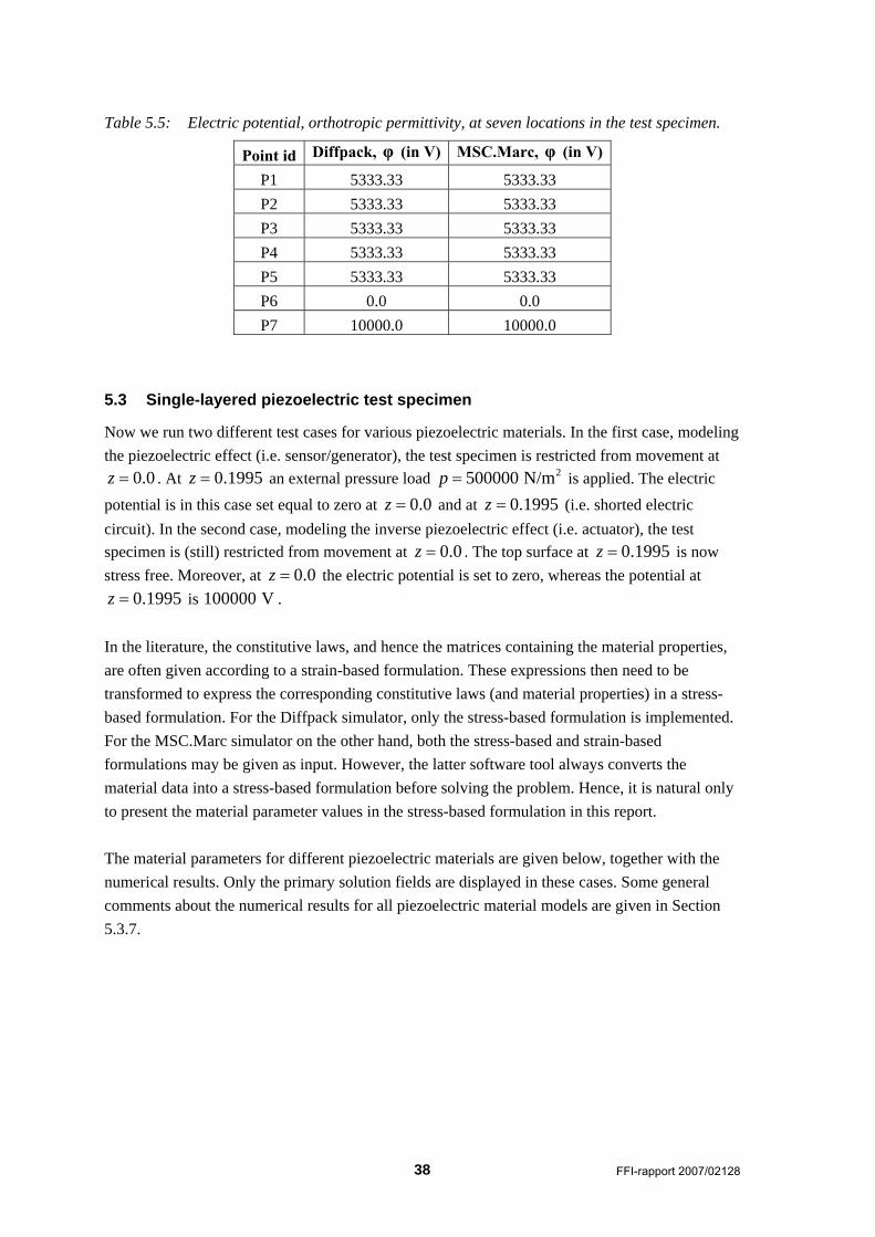
Table 5.7: Quartz, piezoelectric effect; MSC.Marc. Displacement and electric potential at seven locations in the test specimen.
Point id u ( 910−× m) v ( 910−× m) w ( 910−× m) φ (V)
P1 -1.042 0.0989 -5.26 -0.61 P2 0.0 -0.0083 -4.74 0.0 P3 1.042 0.0989 -5.26 0.61 P4 0.0 -1.124 -5.21 0.0 P5 0.0 0.965 -5.31 0.0 P6 0.0 0.0 0.0 0.0 P7 0.0 -0.0258 -9.13 0.0
(a) (b)
(c) (d)
Figure 5.11: Quartz, piezoelectric effect; MSC.Marc. a) displacement in the x direction; b) displacement in the y direction; c) displacement in the z direction; d) electric potential.

42 FFI-rapport 2007/02128
5.3.1.2 Inverse piezoelectric effect
The numerical results are displayed in Table 5.8 and Table 5.9 and in Figure 5.12 and Figure 5.13.
Wed Aug 8 10:24:38 2007
u_1
−4.65e−14
−3.69e−14
−2.73e−14
−1.77e−14
−8.05e−15
1.58e−15
1.12e−14
2.08e−14
3.05e−14
4.01e−14
4.97e−14
XY
Z
0
0.001
0.001995
00.001
0.0020.003
0.0040.005
00.001
0.0020.003
0.0040.005
Wed Aug 8 10:24:49 2007
u_2
−4.91e−14
−3.94e−14
−2.97e−14
−2e−14
−1.04e−14
−6.98e−16
8.98e−15
1.87e−14
2.83e−14
3.8e−14
4.77e−14
XY
Z
0
0.001
0.001995
00.001
0.0020.003
0.0040.005
00.001
0.0020.003
0.0040.005
(a) (b) Wed Aug 8 10:25:01 2007
u_3
−4.98e−13
−4.48e−13
−3.98e−13
−3.49e−13
−2.99e−13
−2.49e−13
−1.99e−13
−1.49e−13
−9.96e−14
−4.98e−14
0
XY
Z
0
0.001
0.001995
00.001
0.0020.003
0.0040.005
00.001
0.0020.003
0.0040.005
Wed Aug 8 10:25:15 2007
phi
0
1e+04
2e+04
3e+04
4e+04
5e+04
6e+04
7e+04
8e+04
9e+04
1e+05
XY
Z
0
0.001
0.001995
00.001
0.0020.003
0.0040.005
00.001
0.0020.003
0.0040.005
(c) (d)
Figure 5.12: Quartz, inverse piezoelectric effect; Diffpack. a) displacement in the x direction; b) displacement in the y direction; c) displacement in the z direction; d) electric potential.

FFI-rapport 2007/02128 43
Table 5.8: Quartz, inverse piezoelectric effect; Diffpack. Displacement and electric potential at seven locations in the test specimen.
Point id u ( 1410−× m) v ( 1410−× m) w ( 1410−× m) φ (V)
P1 -4.54 0.64 -38.16 53333.3 P2 -0.06 0.02 -37.26 53333.3 P3 4.49 0.49 -38.13 53333.3 P4 0.14 -4.73 -37.81 53333.3 P5 -0.11 4.19 -38.53 53333.3 P6 0.0 0.0 0.0 0.0 P7 -0.04 -0.02 -48.03 100000.0
(a) (b)
(c) (d)
Figure 5.13: Quartz, piezoelectric effect; MSC.Marc. a) displacement in the x direction; b) displacement in the y direction; c) displacement in the z direction; d) electric potential.

44 FFI-rapport 2007/02128
Table 5.9: Quartz, inverse piezoelectric effect; MSC.Marc. Displacement and electric potential at seven locations in the test specimen.
Point id u ( 1410−× m) v ( 1410−× m) w ( 1410−× m) φ (V)
P1 -4.49 0.48 -38.14 53333.3 P2 0.0 -0.03 -37.27 53333.3 P3 4.49 0.48 -38.14 53333.3 P4 0.0 -4.77 -37.77 53333.3 P5 0.0 4.23 -38.55 53333.3 P6 0.0 0.0 0.0 0.0 P7 0.0 -0.11 -48.01 100000.0
5.3.2 Langasite
The material parameters for langasite ( 3 5 14La Ga SiO ) are as follows [26;27]:
Mass density: 35743.0 kg/mρ =
Elastic properties:
10 2
18.875 10.475 9.589 0 1.412 010.475 18.875 9.589 0 1.412 09.589 9.589 26.14 0 0 0
10 N/m0 0 0 4.2 0 1.412
1.412 1.412 0 0 5.35 00 0 0 1.412 0 5.35
−⎛ ⎞⎜ ⎟⎜ ⎟⎜ ⎟
= ×⎜ ⎟−⎜ ⎟
⎜ ⎟−⎜ ⎟⎜ ⎟−⎝ ⎠
C . (5.10)
Permittivity:
12
167.5 0 00 167.5 0 10 F/m0 0 448.9
−
⎛ ⎞⎜ ⎟= ×⎜ ⎟⎜ ⎟⎝ ⎠
b . (5.11)
Piezoelectric coupling:
2
0.44 0.44 0 0 0.08 00 0 0 0.44 0 0.08 C/m0 0 0 0 0 0
− −⎛ ⎞⎜ ⎟= ⎜ ⎟⎜ ⎟⎝ ⎠
h . (5.12)
FFI-rapport 2007/02128 45
5.3.2.1 Piezoelectric effect
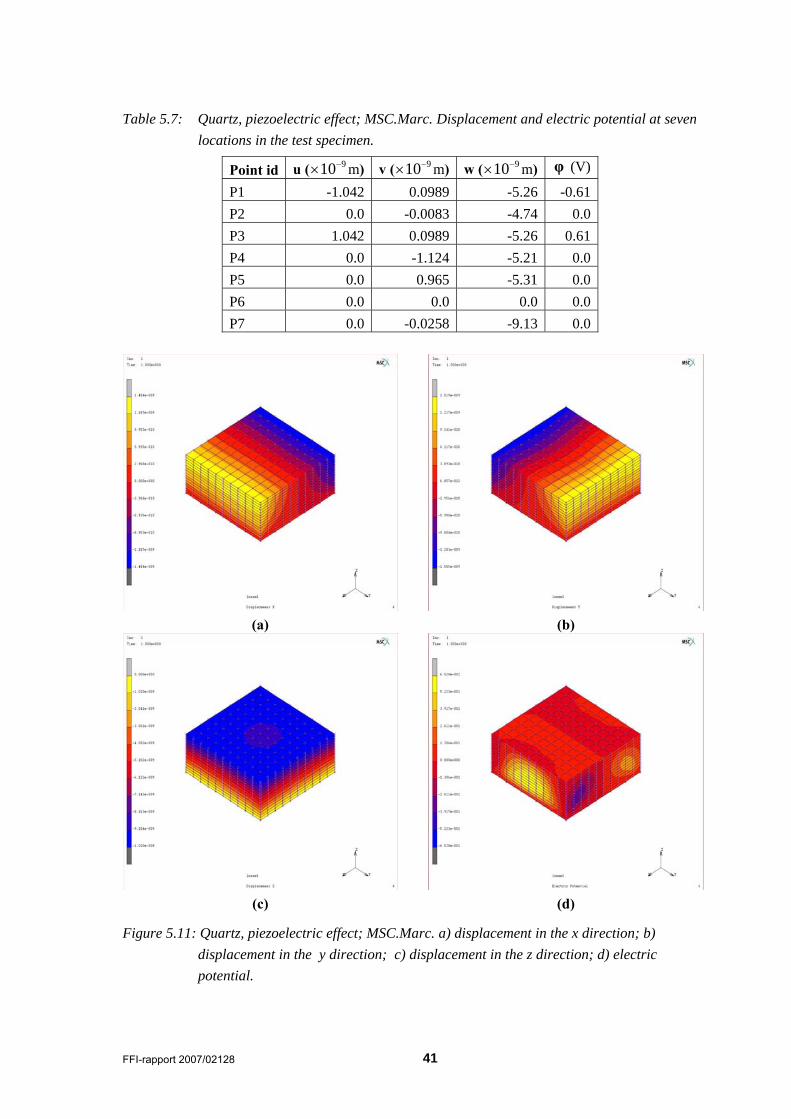
The numerical results are shown in and Table 5.11 and in Figure 5.14 and Figure 5.15.
Wed Aug 8 10:32:34 2007
u_1
−2.18e−09
−1.74e−09
−1.31e−09
−8.7e−10
−4.35e−10
0
4.35e−10
8.7e−10
1.31e−09
1.74e−09
2.18e−09
XY
Z
0
0.001
0.001995
00.001
0.0020.003
0.0040.005
00.001
0.0020.003
0.0040.005
Wed Aug 8 10:32:46 2007
u_2
−2.2e−09
−1.77e−09
−1.33e−09
−8.99e−10
−4.65e−10
−3.07e−11
4.04e−10
8.38e−10
1.27e−09
1.71e−09
2.14e−09
XY
Z
0
0.001
0.001995
00.001
0.0020.003
0.0040.005
00.001
0.0020.003
0.0040.005
(a) (b) Wed Aug 8 10:32:59 2007
u_3
−5.5e−09
−4.95e−09
−4.4e−09
−3.85e−09
−3.3e−09
−2.75e−09
−2.2e−09
−1.65e−09
−1.1e−09
−5.5e−10
0
XY
Z
0
0.001
0.001995
00.001
0.0020.003
0.0040.005
00.001
0.0020.003
0.0040.005
Wed Aug 8 10:33:12 2007
phi
−0.512
−0.41
−0.307
−0.205
−0.102
0
0.102
0.205
0.307
0.41
0.512
XY
Z
0
0.001
0.001995
00.001
0.0020.003
0.0040.005
00.001
0.0020.003
0.0040.005
(c) (d)
Figure 5.14: Langasite, piezoelectric effect; Diffpack. a) displacement in the x direction; b) displacement in the y direction; c) displacement in the z direction; d) electric potential.

46 FFI-rapport 2007/02128
Table 5.10: Langasite, piezoelectric effect; Diffpack. Displacement and electric potential at seven locations in the test specimen.
Point id u ( 910−× m) v ( 910−× m) w ( 910−× m) φ (V)
P1 -1.735 0.128 -2.652 0.382 P2 0.0 -0.021 -2.078 0.0 P3 1.735 0.128 -2.652 -0.382 P4 0.0 -1.835 -2.613 0.0 P5 0.0 1.634 -2.697 0.0 P6 0.0 0.0 0.0 0.0 P7 0.0 -0.046 -4.297 0.0
(a) (b)
(c) (d)
Figure 5.15:Langasite, piezoelectric effect; MSC.Marc. a) displacement in the x direction; b) displacement in the y direction; c) displacement in the z direction; d) electric potential.

FFI-rapport 2007/02128 47
Table 5.11: Langasite, piezoelectric effect; MSC.Marc. Displacement and electric potential at seven locations in the test specimen.
Point id u ( 910−× m) v ( 910−× m) w ( 910−× m) φ (V)
P1 -1.735 0.128 -2.652 0.382 P2 0.0 -0.021 -2.078 0.0 P3 1.735 0.128 -2.652 -0.382 P4 0.0 -1.835 -2.613 0.0 P5 0.0 1.634 -2.697 0.0 P6 0.0 0.0 0.0 0.0 P7 0.0 -0.046 -4.297 0.0
5.3.2.2 Inverse piezoelectric effect
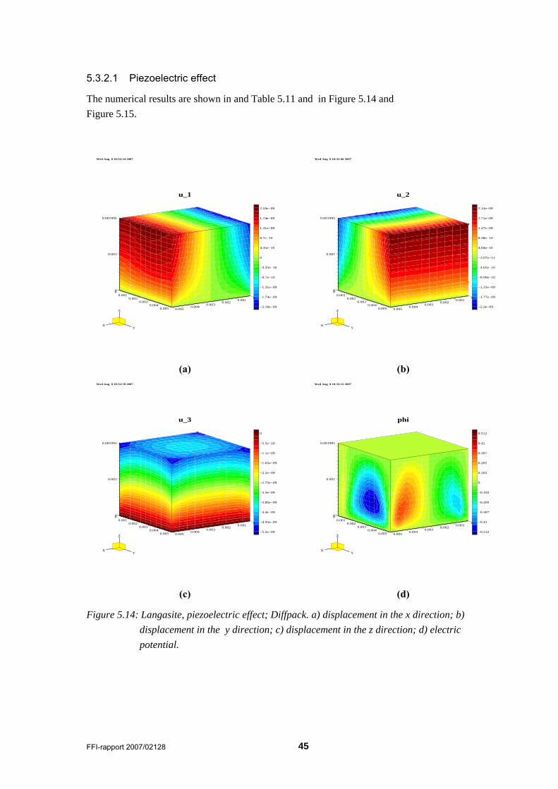
The numerical results are displayed in Table 5.12 and Table 5.13 and in Figure 5.16 and Figure 5.17.
Table 5.12: Langasite, inverse piezoelectric effect; Diffpack. Displacement and electric potential at seven locations in the test specimen.
Point id u ( 1410−× m) v ( 1410−× m) w ( 1410−× m) φ (V)
P1 -17.65 1.12 -37.58 53333.3 P2 -0.08 -0.26 -35.19 53333.3 P3 17.33 0.68 -37.45 53333.3 P4 0.11 -17.53 -36.84 53333.3 P5 0.21 16.82 -38.31 53333.3 P6 0.0 0.0 0.0 0.0 P7 0.02 -0.45 -48.36 100000.0

48 FFI-rapport 2007/02128
Wed Aug 8 10:37:40 2007
u_1
−1.9e−13
−1.52e−13
−1.14e−13
−7.62e−14
−3.84e−14
−6.38e−16
3.71e−14
7.49e−14
1.13e−13
1.5e−13
1.88e−13
XY
Z
0
0.001
0.001995
00.001
0.0020.003
0.0040.005
00.001
0.0020.003
0.0040.005
Wed Aug 8 10:37:50 2007
u_2
−1.96e−13
−1.58e−13
−1.2e−13
−8.26e−14
−4.5e−14
−7.39e−15
3.02e−14
6.79e−14
1.05e−13
1.43e−13
1.81e−13
XY
Z
0
0.001
0.001995
00.001
0.0020.003
0.0040.005
00.001
0.0020.003
0.0040.005
(a) (b) Wed Aug 8 10:38:06 2007
u_3
−5.35e−13
−4.81e−13
−4.28e−13
−3.74e−13
−3.21e−13
−2.67e−13
−2.14e−13
−1.6e−13
−1.07e−13
−5.35e−14
0
XY
Z
0
0.001
0.001995
00.001
0.0020.003
0.0040.005
00.001
0.0020.003
0.0040.005
Wed Aug 8 10:38:18 2007
phi
0
1e+04
2e+04
3e+04
4e+04
5e+04
6e+04
7e+04
8e+04
9e+04
1e+05
XY
Z
0
0.001
0.001995
00.001
0.0020.003
0.0040.005
00.001
0.0020.003
0.0040.005
(c) (d)
Figure 5.16: Langasite, inverse piezoelectric effect; Diffpack. a) displacement in the x direction; b) displacement in the y direction; c) displacement in the z direction; d) electric potential.
FFI-rapport 2007/02128 49
(a) (b)
(c) (d)
Figure 5.17: Langasite, inverse piezoelectric effect; MSC.Marc. a) displacement in the x direction; b) displacement in the y direction; c) displacement in the z direction; d) electric potential.
Table 5.13: Langasite, inverse piezoelectric effect; MSC.Marc. Displacement and electric potential at seven locations in the test specimen.
Point id u ( 1410−× m) v ( 1410−× m) w ( 1410−× m) φ (V)
P1 -17.29 0.93 -37.51 53333.3 P2 0.0 -0.27 -35.18 53333.3 P3 17.29 0.93 -37.51 53333.3 P4 0.0 -17.68 -36.81 53333.3 P5 0.0 16.84 -38.31 53333.3 P6 0.0 0.0 0.0 0.0 P7 0.0 -0.49 -48.25 100000.0

50 FFI-rapport 2007/02128
5.3.3 Lithum niobate
The material parameters for lithium niobate are as follows [26;28]: Mass density: 34700.0 kg/mρ =
Elastic properties:
11 2
2.03 0.53 0.75 0 0.09 00.53 2.03 0.75 0 0.09 00.75 0.75 2.45 0 0 0
10 N/m0 0 0 0.75 0 0.09
0.09 0.09 0 0 0.6 00 0 0 0.09 0 0.06
⎛ ⎞⎜ ⎟−⎜ ⎟⎜ ⎟
= ×⎜ ⎟⎜ ⎟⎜ ⎟−⎜ ⎟⎜ ⎟⎝ ⎠
C . (5.13)
Permittivity:
11
38.9 0 00 38.9 0 10 F/m0 0 25.7
−
⎛ ⎞⎜ ⎟= ×⎜ ⎟⎜ ⎟⎝ ⎠
b . (5.14)
Piezoelectric coupling:
2
0 0 0 2.5 0 3.72.5 2.5 0 0 3.7 0 C/m
0.2 0.2 1.3 0 0 0
−⎛ ⎞⎜ ⎟= −⎜ ⎟⎜ ⎟⎝ ⎠
h . (5.15)
5.3.3.1 Piezoelectric effect
The numerical results are shown in Table 5.14 and Table 5.15 and in Figure 5.18 and Figure 5.19.
Table 5.14: Lithium niobate, piezoelectric effect; Diffpack. Displacement and electric potential at seven locations in the test specimen.
Point id u ( 910−× m) v ( 910−× m) w ( 910−× m) φ (V)
P1 -1.389 -0.010 -2.667 0.458 P2 0.0 -0.001 -2.106 -1.851 P3 1.389 -0.010 -2.667 0.458 P4 0.0 -1.400 -2.656 -0.298 P5 0.0 1.376 -2.672 1.121 P6 0.0 0.0 0.0 0.0 P7 0.0 0.001 -4.302 0.0
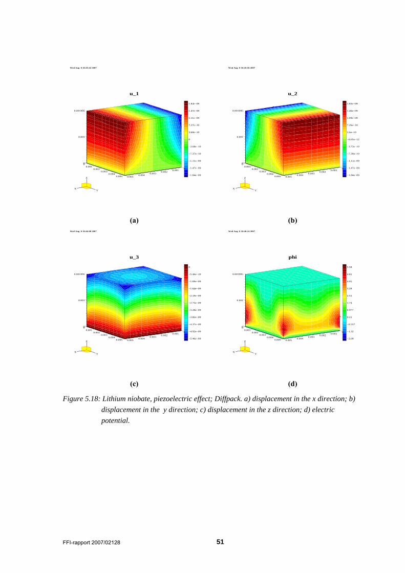
FFI-rapport 2007/02128 51
Wed Aug 8 10:45:42 2007
u_1
−1.84e−09
−1.47e−09
−1.11e−09
−7.37e−10
−3.68e−10
0
3.68e−10
7.37e−10
1.11e−09
1.47e−09
1.84e−09
XY
Z
0
0.001
0.001995
00.001
0.0020.003
0.0040.005
00.001
0.0020.003
0.0040.005
Wed Aug 8 10:45:56 2007
u_2
−1.84e−09
−1.47e−09
−1.11e−09
−7.39e−10
−3.73e−10
−6.65e−12
3.6e−10
7.26e−10
1.09e−09
1.46e−09
1.83e−09
XY
Z
0
0.001
0.001995
00.001
0.0020.003
0.0040.005
00.001
0.0020.003
0.0040.005
(a) (b) Wed Aug 8 10:46:08 2007
u_3
−5.46e−09
−4.92e−09
−4.37e−09
−3.82e−09
−3.28e−09
−2.73e−09
−2.19e−09
−1.64e−09
−1.09e−09
−5.46e−10
0
XY
Z
0
0.001
0.001995
00.001
0.0020.003
0.0040.005
00.001
0.0020.003
0.0040.005
Wed Aug 8 10:46:24 2007
phi
−2.09
−1.32
−0.557
0.21
0.977
1.74
2.51
3.28
4.05
4.81
5.58
XY
Z
0
0.001
0.001995
00.001
0.0020.003
0.0040.005
00.001
0.0020.003
0.0040.005
(c) (d)
Figure 5.18: Lithium niobate, piezoelectric effect; Diffpack. a) displacement in the x direction; b) displacement in the y direction; c) displacement in the z direction; d) electric potential.
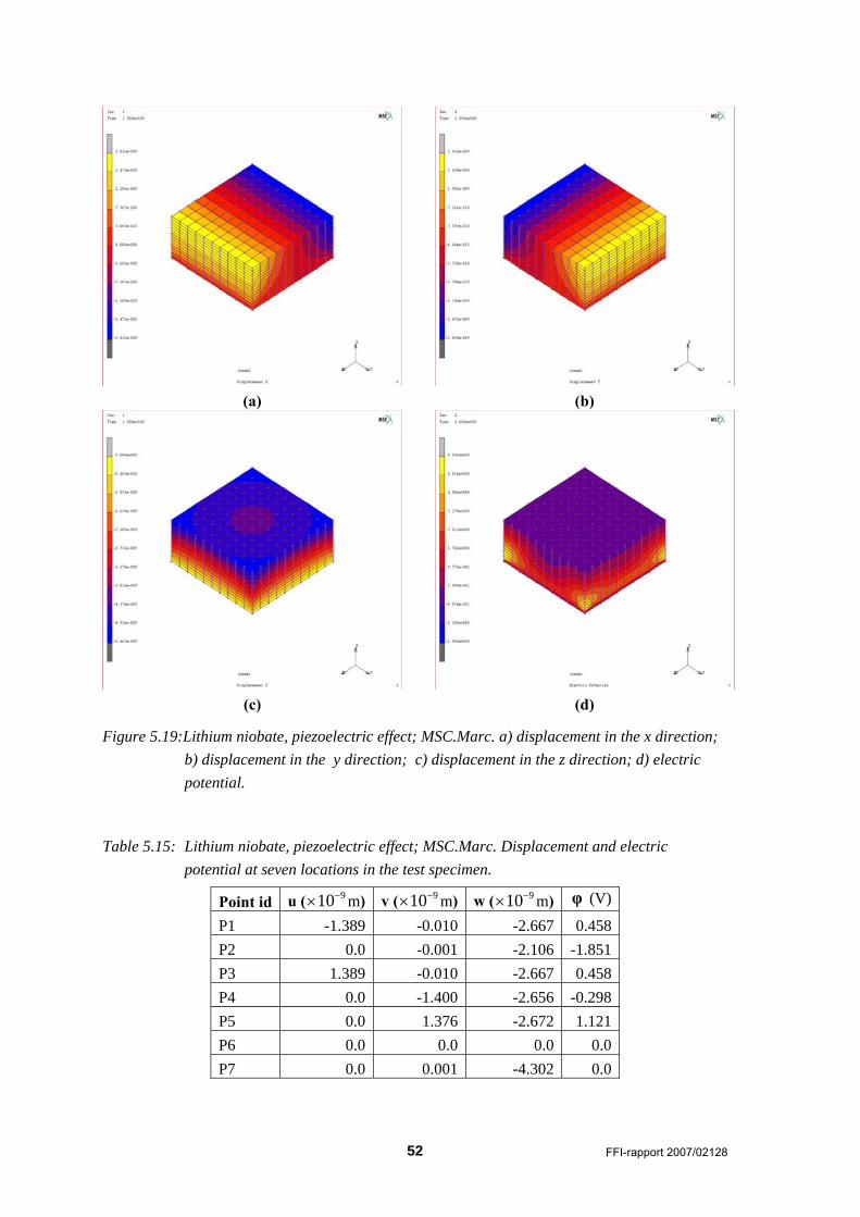
52 FFI-rapport 2007/02128
(a) (b)
(c) (d)
Figure 5.19:Lithium niobate, piezoelectric effect; MSC.Marc. a) displacement in the x direction; b) displacement in the y direction; c) displacement in the z direction; d) electric potential.
Table 5.15: Lithium niobate, piezoelectric effect; MSC.Marc. Displacement and electric potential at seven locations in the test specimen.
Point id u ( 910−× m) v ( 910−× m) w ( 910−× m) φ (V)
P1 -1.389 -0.010 -2.667 0.458 P2 0.0 -0.001 -2.106 -1.851 P3 1.389 -0.010 -2.667 0.458 P4 0.0 -1.400 -2.656 -0.298 P5 0.0 1.376 -2.672 1.121 P6 0.0 0.0 0.0 0.0 P7 0.0 0.001 -4.302 0.0

FFI-rapport 2007/02128 53
5.3.3.2 Inverse piezoelectric effect
The numerical results are displayed in Table 5.16 and Table 5.17 and in Figure 5.20 and Figure 5.21.
Wed Aug 8 10:53:20 2007
u_1
−1.19e−07
−9.55e−08
−7.16e−08
−4.78e−08
−2.39e−08
0
2.39e−08
4.78e−08
7.16e−08
9.55e−08
1.19e−07
XY
Z
0
0.001
0.001995
00.001
0.0020.003
0.0040.005
00.001
0.0020.003
0.0040.005
Wed Aug 8 10:53:30 2007
u_2
−1.19e−07
−9.54e−08
−7.17e−08
−4.79e−08
−2.42e−08
−4.3e−10
2.33e−08
4.71e−08
7.08e−08
9.46e−08
1.18e−07
XY
Z
0
0.001
0.001995
00.001
0.0020.003
0.0040.005
00.001
0.0020.003
0.0040.005
(a) (b) Wed Aug 8 10:53:41 2007
u_3
−6.21e−07
−5.59e−07
−4.97e−07
−4.35e−07
−3.72e−07
−3.1e−07
−2.48e−07
−1.86e−07
−1.24e−07
−6.21e−08
0
XY
Z
0
0.001
0.001995
00.001
0.0020.003
0.0040.005
00.001
0.0020.003
0.0040.005
Wed Aug 8 10:53:53 2007
phi
0
1e+04
2e+04
3e+04
4e+04
5e+04
6e+04
7e+04
8e+04
9e+04
1e+05
XY
Z
0
0.001
0.001995
00.001
0.0020.003
0.0040.005
00.001
0.0020.003
0.0040.005
(c) (d)
Figure 5.20: Lithium niobate, inverse piezoelectric effect; Diffpack. a) displacement in the x direction; b) displacement in the y direction; c) displacement in the z direction; d) electric potential.

54 FFI-rapport 2007/02128
Table 5.16: Lithium niobate, inverse piezoelectric effect; Diffpack. Displacement and electric potential at seven locations in the test specimen.
Point id u ( 710−× m) v ( 710−× m) w ( 710−× m) φ (V)
P1 -0.9 -0.007 -3.15 53363.0 P2 0.0 -0.001 -2.79 53213.4 P3 0.9 -0.007 -3.15 53363.0 P4 0.0 -0.907 -3.14 53314.1 P5 0.0 0.892 -3.15 53406.0 P6 0.0 0.0 0.0 0.0 P7 0.0 0.001 -5.46 100000.0
(a) (b)
(c) (d)
Figure 5.21: Lithium niobate, inverse piezoelectric effect; MSC.Marc. a) displacement in the x direction; b) displacement in the y direction; c) displacement in the z direction; d) electric potential.

FFI-rapport 2007/02128 55
Table 5.17: Lithium niobate, inverse piezoelectric effect; MSC.Marc. Displacement and electric potential at seven locations in the test specimen.
Point id u ( 710−× m) v ( 710−× m) w ( 710−× m) φ (V)
P1 -0.9 -0.007 -3.15 53363.0 P2 0.0 -0.001 -2.79 53213.4 P3 0.9 -0.007 -3.15 53363.0 P4 0.0 -0.907 -3.14 53314.1 P5 0.0 0.892 -3.15 53406.0 P6 0.0 0.0 0.0 0.0 P7 0.0 0.001 -5.46 100000.0
5.3.4 Lithium tantalate
The material properties for lithium tantalate are as follows [26;28]: Mass density: 37450.0 kg/mρ =
Elastic properties:
11 2
2.33 0.47 0.8 0 0.11 00.47 2.33 0.8 0 0.11 00.8 0.8 2.75 0 0 0
10 N/m0 0 0 0.93 0 0.11
0.11 0.11 0 0 0.94 00 0 0 0.11 0 0.94
−⎛ ⎞⎜ ⎟⎜ ⎟⎜ ⎟
= ×⎜ ⎟−⎜ ⎟
⎜ ⎟−⎜ ⎟⎜ ⎟−⎝ ⎠
C . (5.16)
Remark that Yang [26] has reported another value for component 33C ( 11 22.45 10 N/m= × ),
although referring to the work by Warner et al. [28]. Permittivity:
11
36.3 0 00 36.3 0 10 F/m0 0 38.2
−
⎛ ⎞⎜ ⎟= ×⎜ ⎟⎜ ⎟⎝ ⎠
b . (5.17)
Piezoelectric coupling:
2
0 0 0 1.6 0 2.61.6 1.6 0 0 2.6 0 C/m0 0 1.9 0 0 0
−⎛ ⎞⎜ ⎟= −⎜ ⎟⎜ ⎟⎝ ⎠
h . (5.18)

56 FFI-rapport 2007/02128
5.3.4.1 Piezoelectric effect
The numerical results are shown in and Table 5.19 and in Figure 5.22 and Figure 5.23.
Wed Aug 8 11:11:14 2007
u_1
−1.55e−09
−1.24e−09
−9.32e−10
−6.21e−10
−3.11e−10
0
3.11e−10
6.21e−10
9.32e−10
1.24e−09
1.55e−09
XY
Z
0
0.001
0.001995
00.001
0.0020.003
0.0040.005
00.001
0.0020.003
0.0040.005
Wed Aug 8 11:11:24 2007
u_2
−1.56e−09
−1.25e−09
−9.37e−10
−6.25e−10
−3.14e−10
−2.23e−12
3.09e−10
6.21e−10
9.32e−10
1.24e−09
1.56e−09
XY
Z
0
0.001
0.001995
00.001
0.0020.003
0.0040.005
00.001
0.0020.003
0.0040.005
(a) (b) Wed Aug 8 11:11:36 2007
u_3
−4.83e−09
−4.35e−09
−3.87e−09
−3.38e−09
−2.9e−09
−2.42e−09
−1.93e−09
−1.45e−09
−9.66e−10
−4.83e−10
0
XY
Z
0
0.001
0.001995
00.001
0.0020.003
0.0040.005
00.001
0.0020.003
0.0040.005
Wed Aug 8 11:11:54 2007
phi
−0.435
−0.174
0.0873
0.348
0.609
0.87
1.13
1.39
1.65
1.91
2.17
XY
Z
0
0.001
0.001995
00.001
0.0020.003
0.0040.005
00.001
0.0020.003
0.0040.005
(c) (d)
Figure 5.22: Lithium tantalate, piezoelectric effect; Diffpack. a) displacement in the x direction; b) displacement in the y direction; c) displacement in the z direction; d) electric potential.

FFI-rapport 2007/02128 57
Table 5.18: Lithium tantalate, piezoelectric effect; Diffpack. Displacement and electric potential at seven locations in the test specimen.
Point id u ( 910−× m) v ( 910−× m) w ( 910−× m) φ (V)
P1 -1.138 0.037 -2.346 0.462 P2 0.0 -0.003 -1.835 -0.363 P3 1.138 0.037 -2.346 0.462 P4 0.0 -1.170 -2.321 0.044 P5 0.0 1.105 -2.371 0.921 P6 0.0 0.0 0.0 0.0 P7 0.0 -0.010 -3.746 0.0
(a) (b)
(c) (d)
Figure 5.23: Lithium tantalate, piezoelectric effect; MSC.Marc. a) displacement in the x direction; b) displacement in the y direction; c) displacement in the z direction; d) electric potential.
58 FFI-rapport 2007/02128
Table 5.19: Lithium tantalate, piezoelectric effect; MSC.Marc. Displacement and electric potential at seven locations in the test specimen.
Point id u ( 910−× m) v ( 910−× m) w ( 910−× m) φ (V)
P1 -1.138 0.037 -2.346 0.462 P2 0.0 -0.003 -1.835 -0.363 P3 1.138 0.037 -2.346 0.462 P4 0.0 -1.170 -2.321 0.044 P5 0.0 1.105 -2.371 0.921 P6 0.0 0.0 0.0 0.0 P7 0.0 -0.010 -3.746 0.0
5.3.4.2 Inverse piezoelectric effect
The numerical results are displayed in Table 5.20 and Table 5.21 and in Figure 5.24 and Figure 5.25.
Table 5.20: Lithium tantalate, inverse piezoelectric effect; Diffpack. Displacement and electric potential at seven locations in the test specimen.
Point id u ( 710−× m) v ( 710−× m) w ( 710−× m) φ (V)
P1 -2.167 0.070 -4.467 53421.4 P2 0.0 -0.005 -3.494 53264.4 P3 2.167 0.070 -4.467 53421.4 P4 0.0 -2.228 -4.419 53341.8 P5 0.0 2.104 -4.516 53508.8 P6 0.0 0.0 0.0 0.0 P7 0.0 -0.018 -7.133 100000.0
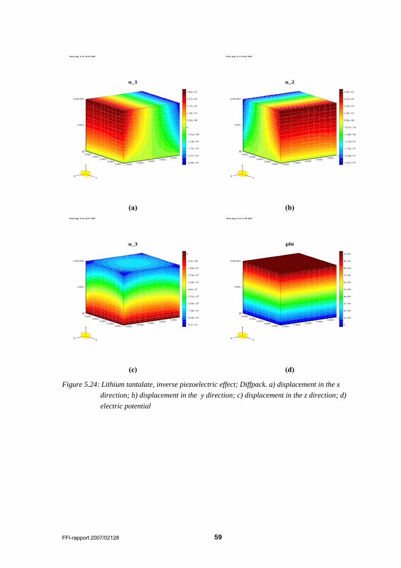
FFI-rapport 2007/02128 59
Wed Aug 8 11:16:34 2007
u_1
−2.96e−07
−2.37e−07
−1.77e−07
−1.18e−07
−5.92e−08
0
5.92e−08
1.18e−07
1.77e−07
2.37e−07
2.96e−07
XY
Z
0
0.001
0.001995
00.001
0.0020.003
0.0040.005
00.001
0.0020.003
0.0040.005
Wed Aug 8 11:16:45 2007
u_2
−2.97e−07
−2.38e−07
−1.78e−07
−1.19e−07
−5.98e−08
−4.25e−10
5.89e−08
1.18e−07
1.78e−07
2.37e−07
2.96e−07
XY
Z
0
0.001
0.001995
00.001
0.0020.003
0.0040.005
00.001
0.0020.003
0.0040.005
(a) (b) Wed Aug 8 11:16:57 2007
u_3
−9.2e−07
−8.28e−07
−7.36e−07
−6.44e−07
−5.52e−07
−4.6e−07
−3.68e−07
−2.76e−07
−1.84e−07
−9.2e−08
0
XY
Z
0
0.001
0.001995
00.001
0.0020.003
0.0040.005
00.001
0.0020.003
0.0040.005
Wed Aug 8 11:17:09 2007
phi
0
1e+04
2e+04
3e+04
4e+04
5e+04
6e+04
7e+04
8e+04
9e+04
1e+05
XY
Z
0
0.001
0.001995
00.001
0.0020.003
0.0040.005
00.001
0.0020.003
0.0040.005
(c) (d)
Figure 5.24: Lithium tantalate, inverse piezoelectric effect; Diffpack. a) displacement in the x direction; b) displacement in the y direction; c) displacement in the z direction; d) electric potential
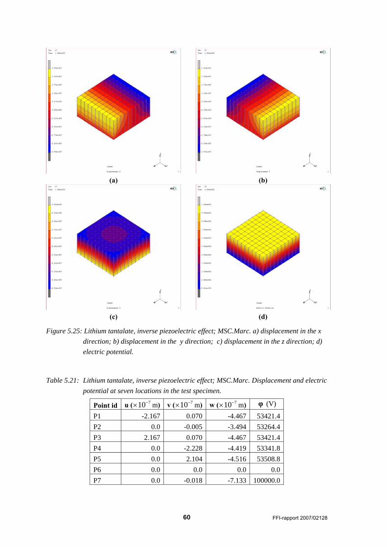
60 FFI-rapport 2007/02128
(a) (b)
(c) (d)
Figure 5.25: Lithium tantalate, inverse piezoelectric effect; MSC.Marc. a) displacement in the x direction; b) displacement in the y direction; c) displacement in the z direction; d) electric potential.
Table 5.21: Lithium tantalate, inverse piezoelectric effect; MSC.Marc. Displacement and electric potential at seven locations in the test specimen.
Point id u ( 710−× m) v ( 710−× m) w ( 710−× m) φ (V)
P1 -2.167 0.070 -4.467 53421.4 P2 0.0 -0.005 -3.494 53264.4 P3 2.167 0.070 -4.467 53421.4 P4 0.0 -2.228 -4.419 53341.8 P5 0.0 2.104 -4.516 53508.8 P6 0.0 0.0 0.0 0.0 P7 0.0 -0.018 -7.133 100000.0
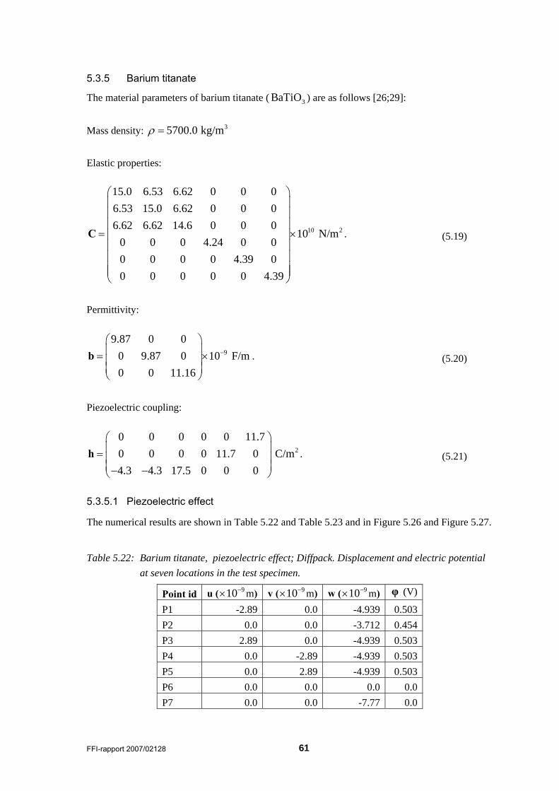
FFI-rapport 2007/02128 61
5.3.5 Barium titanate
The material parameters of barium titanate ( 3BaTiO ) are as follows [26;29]:
Mass density: 35700.0 kg/mρ =
Elastic properties:
10 2
15.0 6.53 6.62 0 0 06.53 15.0 6.62 0 0 06.62 6.62 14.6 0 0 0
10 N/m0 0 0 4.24 0 00 0 0 0 4.39 00 0 0 0 0 4.39
⎛ ⎞⎜ ⎟⎜ ⎟⎜ ⎟
= ×⎜ ⎟⎜ ⎟⎜ ⎟⎜ ⎟⎜ ⎟⎝ ⎠
C . (5.19)
Permittivity:
9
9.87 0 00 9.87 0 10 F/m0 0 11.16
−
⎛ ⎞⎜ ⎟= ×⎜ ⎟⎜ ⎟⎝ ⎠
b . (5.20)
Piezoelectric coupling:
2
0 0 0 0 0 11.70 0 0 0 11.7 0 C/m4.3 4.3 17.5 0 0 0
⎛ ⎞⎜ ⎟= ⎜ ⎟⎜ ⎟− −⎝ ⎠
h . (5.21)
5.3.5.1 Piezoelectric effect
The numerical results are shown in Table 5.22 and Table 5.23 and in Figure 5.26 and Figure 5.27.
Table 5.22: Barium titanate, piezoelectric effect; Diffpack. Displacement and electric potential at seven locations in the test specimen.
Point id u ( 910−× m) v ( 910−× m) w ( 910−× m) φ (V)
P1 -2.89 0.0 -4.939 0.503 P2 0.0 0.0 -3.712 0.454 P3 2.89 0.0 -4.939 0.503 P4 0.0 -2.89 -4.939 0.503 P5 0.0 2.89 -4.939 0.503 P6 0.0 0.0 0.0 0.0 P7 0.0 0.0 -7.77 0.0

62 FFI-rapport 2007/02128
Wed Aug 8 12:27:18 2007
u_1
−3.69e−09
−2.96e−09
−2.22e−09
−1.48e−09
−7.39e−10
0
7.39e−10
1.48e−09
2.22e−09
2.96e−09
3.69e−09
XY
Z
0
0.001
0.001995
00.001
0.0020.003
0.0040.005
00.001
0.0020.003
0.0040.005
Wed Aug 8 12:27:31 2007
u_2
−3.69e−09
−2.96e−09
−2.22e−09
−1.48e−09
−7.39e−10
0
7.39e−10
1.48e−09
2.22e−09
2.96e−09
3.69e−09
XY
Z
0
0.001
0.001995
00.001
0.0020.003
0.0040.005
00.001
0.0020.003
0.0040.005
(a) (b) Wed Aug 8 12:27:43 2007
u_3
−1.03e−08
−9.29e−09
−8.26e−09
−7.23e−09
−6.2e−09
−5.16e−09
−4.13e−09
−3.1e−09
−2.07e−09
−1.03e−09
0
XY
Z
0
0.001
0.001995
00.001
0.0020.003
0.0040.005
00.001
0.0020.003
0.0040.005
Wed Aug 8 12:27:57 2007
phi
0
0.081
0.162
0.243
0.324
0.405
0.486
0.567
0.648
0.729
0.81
XY
Z
0
0.001
0.001995
00.001
0.0020.003
0.0040.005
00.001
0.0020.003
0.0040.005
(c) (d)
Figure 5.26: Barium titanate, piezoelectric effect; Diffpack. a) displacement in the x direction; b) displacement in the y direction; c) displacement in the z direction; d) electric potential.

FFI-rapport 2007/02128 63
(a) (b)
(c) (d)
Figure 5.27:Barium titanate, piezoelectric effect; MSC.Marc. a) displacement in the x direction; b) displacement in the y direction; c) displacement in the z direction; d) electric potential.
Table 5.23: Barium titanate, piezoelectric effect; MSC.Marc. Displacement and electric potential at seven locations in the test specimen.
Point id u ( 910−× m) v ( 910−× m) w ( 910−× m) φ (V)
P1 -2.89 0.0 -4.939 0.503 P2 0.0 0.0 -3.712 0.454 P3 2.89 0.0 -4.939 0.503 P4 0.0 -2.89 -4.939 0.503 P5 0.0 2.89 -4.939 0.503 P6 0.0 0.0 0.0 0.0 P7 0.0 0.0 -7.77 0.0
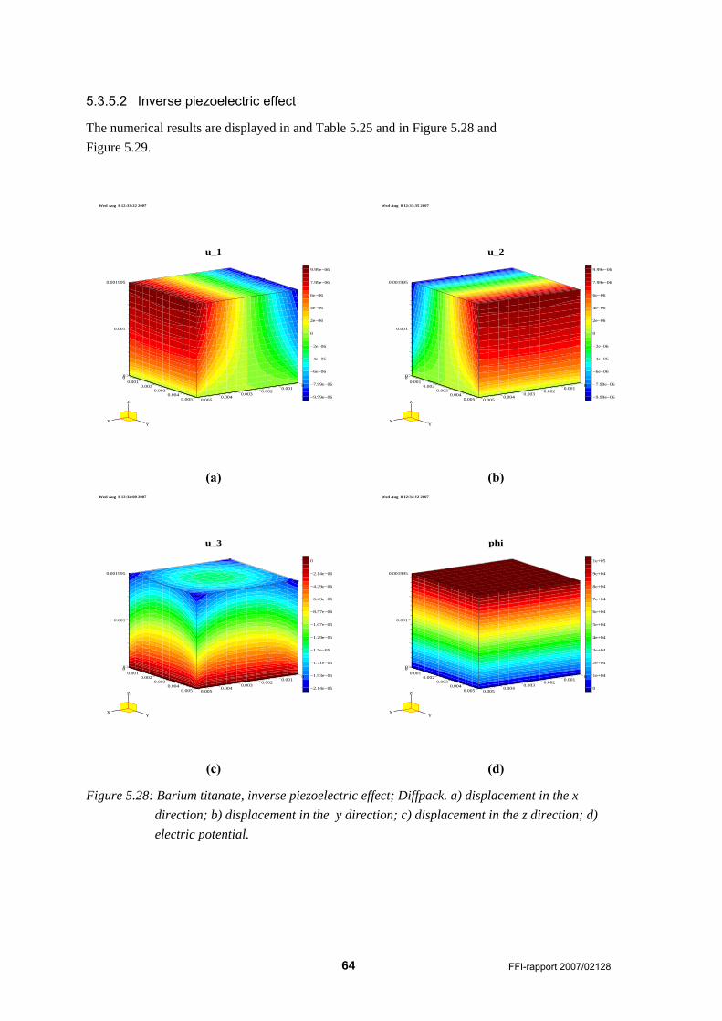
64 FFI-rapport 2007/02128
5.3.5.2 Inverse piezoelectric effect
The numerical results are displayed in and Table 5.25 and in Figure 5.28 and Figure 5.29.
Wed Aug 8 12:33:22 2007
u_1
−9.99e−06
−7.99e−06
−6e−06
−4e−06
−2e−06
0
2e−06
4e−06
6e−06
7.99e−06
9.99e−06
XY
Z
0
0.001
0.001995
00.001
0.0020.003
0.0040.005
00.001
0.0020.003
0.0040.005
Wed Aug 8 12:33:35 2007
u_2
−9.99e−06
−7.99e−06
−6e−06
−4e−06
−2e−06
0
2e−06
4e−06
6e−06
7.99e−06
9.99e−06
XY
Z
0
0.001
0.001995
00.001
0.0020.003
0.0040.005
00.001
0.0020.003
0.0040.005
(a) (b) Wed Aug 8 12:34:00 2007
u_3
−2.14e−05
−1.93e−05
−1.71e−05
−1.5e−05
−1.29e−05
−1.07e−05
−8.57e−06
−6.43e−06
−4.29e−06
−2.14e−06
0
XY
Z
0
0.001
0.001995
00.001
0.0020.003
0.0040.005
00.001
0.0020.003
0.0040.005
Wed Aug 8 12:34:12 2007
phi
0
1e+04
2e+04
3e+04
4e+04
5e+04
6e+04
7e+04
8e+04
9e+04
1e+05
XY
Z
0
0.001
0.001995
00.001
0.0020.003
0.0040.005
00.001
0.0020.003
0.0040.005
(c) (d)
Figure 5.28: Barium titanate, inverse piezoelectric effect; Diffpack. a) displacement in the x direction; b) displacement in the y direction; c) displacement in the z direction; d) electric potential.
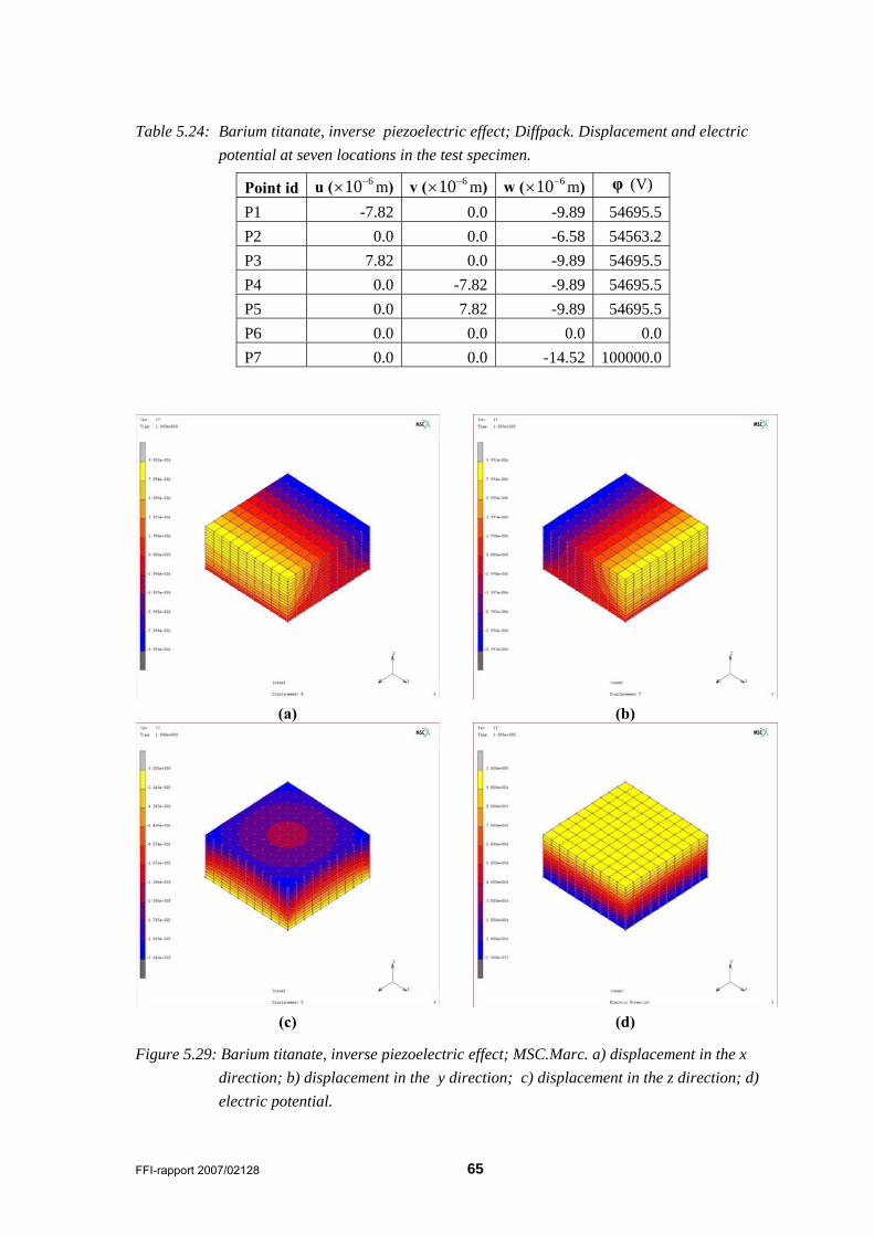
FFI-rapport 2007/02128 65
Table 5.24: Barium titanate, inverse piezoelectric effect; Diffpack. Displacement and electric potential at seven locations in the test specimen.
Point id u ( 610−× m) v ( 610−× m) w ( 610−× m) φ (V)
P1 -7.82 0.0 -9.89 54695.5 P2 0.0 0.0 -6.58 54563.2 P3 7.82 0.0 -9.89 54695.5 P4 0.0 -7.82 -9.89 54695.5 P5 0.0 7.82 -9.89 54695.5 P6 0.0 0.0 0.0 0.0 P7 0.0 0.0 -14.52 100000.0
(a) (b)
(c) (d)
Figure 5.29: Barium titanate, inverse piezoelectric effect; MSC.Marc. a) displacement in the x direction; b) displacement in the y direction; c) displacement in the z direction; d) electric potential.

66 FFI-rapport 2007/02128
Table 5.25: Barium titanate, inverse piezoelectric effect; MSC.Marc. Displacement and electric potential at seven locations in the test specimen.
Point id u ( 610−× m) v ( 610−× m) w ( 610−× m) φ (V)
P1 -7.82 0.0 -9.89 54695.5 P2 0.0 0.0 -6.58 54563.2 P3 7.82 0.0 -9.89 54695.5 P4 0.0 -7.82 -9.89 54695.5 P5 0.0 7.82 -9.89 54695.5 P6 0.0 0.0 0.0 0.0 P7 0.0 0.0 -14.52 100000.0
5.3.6 Lead-zirconate-titanate (PZT) – PZT-4
PZT-4 is a type of lead zirconate titanate, which is a ceramic man-made piezoelectric material. The material parameters for PZT-4 are as follows [26;29]: Mass density: 37500.0 kg/mρ =
Elastic properties:
10 2
13.9 7.78 7.40 0 0 07.78 13.9 7.40 0 0 07.40 7.40 11.5 0 0 0
10 N/m0 0 0 3.06 0 00 0 0 0 2.56 00 0 0 0 0 2.56
⎛ ⎞⎜ ⎟⎜ ⎟⎜ ⎟
= ×⎜ ⎟⎜ ⎟⎜ ⎟⎜ ⎟⎜ ⎟⎝ ⎠
C . (5.22)
Permittivity:
9
6.46 0 00 6.46 0 10 F/m0 0 5.62
−
⎛ ⎞⎜ ⎟= ×⎜ ⎟⎜ ⎟⎝ ⎠
b . (5.23)
Piezoelectric coupling:
2
0 0 0 0 0 12.70 0 0 0 12.7 0 C/m5.2 5.2 15.1 0 0 0
⎛ ⎞⎜ ⎟= ⎜ ⎟⎜ ⎟− −⎝ ⎠
h . (5.24)
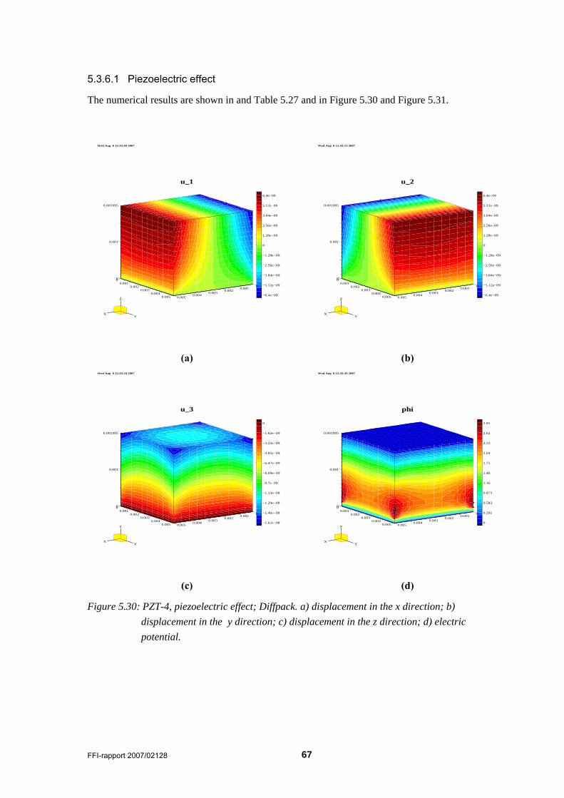
FFI-rapport 2007/02128 67
5.3.6.1 Piezoelectric effect
The numerical results are shown in and Table 5.27 and in Figure 5.30 and Figure 5.31.
Wed Aug 8 12:43:04 2007
u_1
−6.4e−09
−5.12e−09
−3.84e−09
−2.56e−09
−1.28e−09
0
1.28e−09
2.56e−09
3.84e−09
5.12e−09
6.4e−09
XY
Z
0
0.001
0.001995
00.001
0.0020.003
0.0040.005
00.001
0.0020.003
0.0040.005
Wed Aug 8 12:43:13 2007
u_2
−6.4e−09
−5.12e−09
−3.84e−09
−2.56e−09
−1.28e−09
0
1.28e−09
2.56e−09
3.84e−09
5.12e−09
6.4e−09
XY
Z
0
0.001
0.001995
00.001
0.0020.003
0.0040.005
00.001
0.0020.003
0.0040.005
(a) (b) Wed Aug 8 12:43:24 2007
u_3
−1.62e−08
−1.46e−08
−1.29e−08
−1.13e−08
−9.7e−09
−8.09e−09
−6.47e−09
−4.85e−09
−3.23e−09
−1.62e−09
0
XY
Z
0
0.001
0.001995
00.001
0.0020.003
0.0040.005
00.001
0.0020.003
0.0040.005
Wed Aug 8 12:43:39 2007
phi
0
0.291
0.582
0.873
1.16
1.46
1.75
2.04
2.33
2.62
2.91
XY
Z
0
0.001
0.001995
00.001
0.0020.003
0.0040.005
00.001
0.0020.003
0.0040.005
(c) (d)
Figure 5.30: PZT-4, piezoelectric effect; Diffpack. a) displacement in the x direction; b) displacement in the y direction; c) displacement in the z direction; d) electric potential.
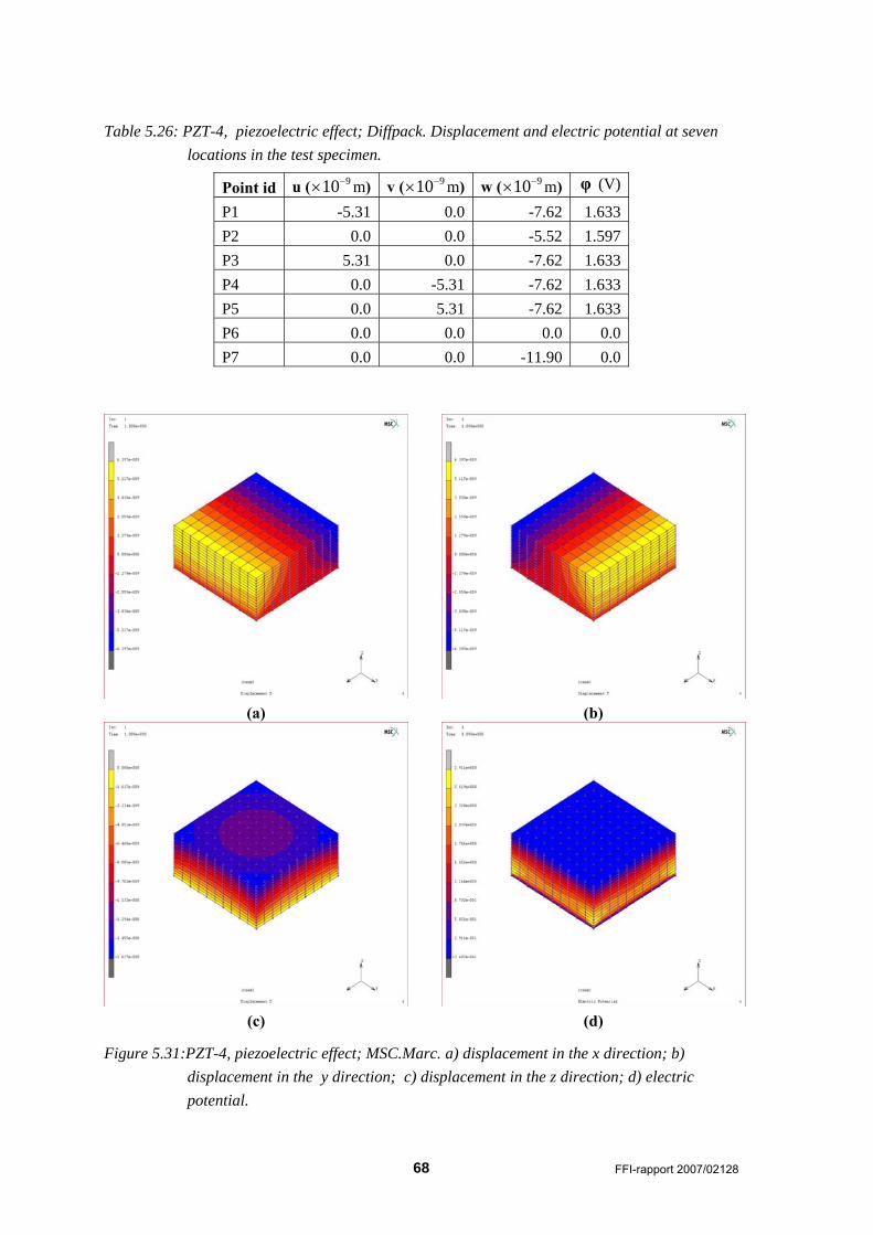
68 FFI-rapport 2007/02128
Table 5.26: PZT-4, piezoelectric effect; Diffpack. Displacement and electric potential at seven locations in the test specimen.
Point id u ( 910−× m) v ( 910−× m) w ( 910−× m) φ (V)
P1 -5.31 0.0 -7.62 1.633 P2 0.0 0.0 -5.52 1.597 P3 5.31 0.0 -7.62 1.633 P4 0.0 -5.31 -7.62 1.633 P5 0.0 5.31 -7.62 1.633 P6 0.0 0.0 0.0 0.0 P7 0.0 0.0 -11.90 0.0
(a) (b)
(c) (d)
Figure 5.31:PZT-4, piezoelectric effect; MSC.Marc. a) displacement in the x direction; b) displacement in the y direction; c) displacement in the z direction; d) electric potential.

FFI-rapport 2007/02128 69
Table 5.27: PZT-4, piezoelectric effect; MSC.Marc. Displacement and electric potential at seven locations in the test specimen.
Point id u ( 910−× m) v ( 910−× m) w ( 910−× m) φ (V)
P1 -5.31 0.0 -7.62 1.633 P2 0.0 0.0 -5.52 1.597 P3 5.31 0.0 -7.62 1.633 P4 0.0 -5.31 -7.62 1.633 P5 0.0 5.31 -7.62 1.633 P6 0.0 0.0 0.0 0.0 P7 0.0 0.0 -11.90 0.0
5.3.6.2 Inverse piezoelectric effect
The numerical results are displayed in Table 5.28 and Table 5.29 and in Figure 5.32 and Figure 5.33.
Table 5.28: PZT-4, inverse piezoelectric effect; Diffpack. Displacement and electric potential at seven locations in the test specimen.
Point id u ( 510−× m) v ( 510−× m) w ( 510−× m) φ (V)
P1 -1.24 0.0 -1.40 57130.0 P2 0.0 0.0 -0.91 57045.1 P3 1.24 0.0 -1.40 57130.0 P4 0.0 -1.24 -1.40 57130.0 P5 0.0 1.24 -1.40 57130.0 P6 0.0 0.0 0.0 0.0 P7 0.0 0.0 -2.06 100000.0
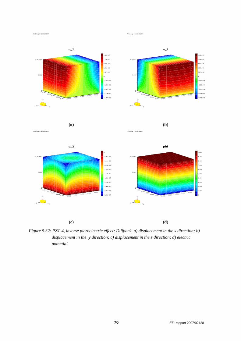
70 FFI-rapport 2007/02128
Wed Aug 8 12:57:24 2007
u_1
−1.49e−05
−1.19e−05
−8.92e−06
−5.95e−06
−2.97e−06
0
2.97e−06
5.95e−06
8.92e−06
1.19e−05
1.49e−05
XY
Z
0
0.001
0.001995
00.001
0.0020.003
0.0040.005
00.001
0.0020.003
0.0040.005
Wed Aug 8 12:57:36 2007
u_2
−1.49e−05
−1.19e−05
−8.92e−06
−5.95e−06
−2.97e−06
0
2.97e−06
5.95e−06
8.92e−06
1.19e−05
1.49e−05
XY
Z
0
0.001
0.001995
00.001
0.0020.003
0.0040.005
00.001
0.0020.003
0.0040.005
(a) (b) Wed Aug 8 12:58:01 2007
u_3
−3.05e−05
−2.75e−05
−2.44e−05
−2.14e−05
−1.83e−05
−1.53e−05
−1.22e−05
−9.16e−06
−6.11e−06
−3.05e−06
0
XY
Z
0
0.001
0.001995
00.001
0.0020.003
0.0040.005
00.001
0.0020.003
0.0040.005
Wed Aug 8 12:58:14 2007
phi
0
1e+04
2e+04
3e+04
4e+04
5e+04
6e+04
7e+04
8e+04
9e+04
1e+05
XY
Z
0
0.001
0.001995
00.001
0.0020.003
0.0040.005
00.001
0.0020.003
0.0040.005
(c) (d)
Figure 5.32: PZT-4, inverse piezoelectric effect; Diffpack. a) displacement in the x direction; b) displacement in the y direction; c) displacement in the z direction; d) electric potential.

FFI-rapport 2007/02128 71
(a) (b)
(c) (d)
Figure 5.33: PZT-4, inverse piezoelectric effect; MSC.Marc. a) displacement in the x direction; b) displacement in the y direction; c) displacement in the z direction; d) electric potential.
Table 5.29: PZT-4, inverse piezoelectric effect; MSC.Marc. Displacement and electric potential at seven locations in the test specimen.
Point id u ( 510−× m) v ( 510−× m) w ( 510−× m) φ (V)
P1 -1.24 0.0 -1.40 57130.0 P2 0.0 0.0 -0.91 57045.1 P3 1.24 0.0 -1.40 57130.0 P4 0.0 -1.24 -1.40 57130.0 P5 0.0 1.24 -1.40 57130.0 P6 0.0 0.0 0.0 0.0 P7 0.0 0.0 -2.06 100000.0

72 FFI-rapport 2007/02128
5.3.7 Concluding remarks for the piezoelectric material cases
The numerical results from the simulations in Diffpack and in MSC.Marc agree very well for all the presented piezoelectric materials test cases. The best agreement is generally found for the test cases simulating the piezoelectric effect; some minor differences are observed for the displacements for quartz and langasite in simulating the inverse piezoelectric effect, see Table 5.8 and Table 5.9, and Table 5.12 and Table 5.13, respectively. For the Diffpack simulator more iterations were needed for obtaining the same error tolerance value for the ceramic material compared to the other materials. This may be related to the elastic material properties being transversely isotropic for ceramic materials. For the other materials tested, the elastic properties are anisotropic, with a coupling (i.e. values different from zero) between the normal stresses and shear strains. Moreover, convergence problems were experienced when simulating a PZT-5H ceramic material [26;30] in Diffpack; this material test case is not included in this report. In all cases a standard conjugate gradient solver has been applied for solving the linear systems involved. The iterative solution method presented in Section 4.1.3, hence does not seem to be fully appropriate for all ceramic piezoelectric materials. From additional tests it seems that the large values in the piezoelectric coupling matrix, related to the poling direction, and the high permittivity values cause the numerical problems. The same numerical problems did not occur when simulating the same problem (i.e. for the PZT-5H material) in MSC.Marc.
6 Summary and future work In this report the aim has been on numerical modeling of piezoelectricity. Basic knowledge of piezoelectricity has been presented, with focus on the mathematical formulation and computer implementation. Two different simulators have been implemented and applied for various piezoelectric materials. Both the piezoelectric effect and the inverse piezoelectric effect have been simulated for all materials. Comparison of the numerical results shows very good agreement. The main reason for implementing two different simulators has been for verification of the code implementation, as well as for increasing the general understanding of the problem. Simulation in Diffpack requires some low-level programming. New classes need to be created for the particular problem, and modifications need to be done for already existing code. Moreover, the integral expressions, which contain the most problem specific part, need to be established and implemented. Details are found in Section 4.1. Such code development is quite time consuming and error prone. However, standard simulators already exist in Diffpack. Hence, a lot of the “standard” code lines can be reused for this particular problem. Another advantage is that we have full control of the implementation, and may easily make adjustments and extensions, when needed. MSC.Marc on the other hand, is more an application software, meaning that all low-level details are hidden to the front-end user. Moreover, efficient solution algorithms are already implemented.

FFI-rapport 2007/02128 73
The advantage of this type of software tools is that we can apply a robust an well tested software for complex problems quite fast. The only programming requirement is establishing an input file. The disadvantage is that a lot of details are hidden inside a “black box”. Some misunderstanding and confusion about the input parameters and calculated results may be experienced. There is very good agreement between the numerical results calculated in the two software tools for all test cases presented in this report. However, some convergence problems occurred in the Diffpack simulator for one ceramic material case. For piezoelectric materials with large values in the piezoelectricity matrix related to the poling direction, and with high permittivity values (compared to the other materials considered), such as the PZT-5H material [26;30], the suggested iterative solution method seems not to be fully appropriate. More research must therefore be done for making the Diffpack simulator applicable to such material cases. The same convergence problems have not been experienced for the MSC.Marc solver. Further work will focus on developing and extending the simulators to also include more advanced, multi-layered piezoelectric elements. Another advanced, future application may be to include piezoelectric material into an elastic composite material. Moreover, the simulation results in this report have been restricted to a static situation only. The piezoelectric effect as a function of time can be of interest. It would, for instance, be interesting to simulate and study the electric field distribution in a free vibrating element. In summary, the exercise of developing two different simulators for the piezoelectricity problem has been very fruitful. It has increased the understanding of the problem and the phenomenon of piezoelectricity, as well as clarified the possibilities and restrictions of the current software tools. In addition, the employed software codes have been verified.
Acknowledgements The author will thank Hege Kristin Jødahl (FFI) and John Fredrik Moxnes (FFI) for reading the manuscript, and for giving very useful input and suggesting improvements.
74 FFI-rapport 2007/02128
Appendix A Constitutive laws In previous sections the constitutive laws, including the piezoelectric coupling term, are expressed both using the tensor notation and the matrix-vector notation. In this section we give some more details about the relationship between the two notations. In structural engineering Hooke’s generalized law expresses the stresses as a product of material stiffness coefficients and the strain values. The “inverse Hooke’s law” then expresses the strains as a product of the compliance values and the stresses. Although the former variant is normally used in defining the constitutive law for elasticity problems, this latter variant is often applied in describing the constitutive law for piezoelectricity. It should, however, be mentioned that there are several ways of formulating the constitutive laws for piezoelectricity. Only two variants are included in this report, starting with a stress-based formulation.
A.1 The stress-based constitutive laws
A.1.1 Tensor notation
In tensor notation, and applying index notation, the stress-based constitutive laws for piezoelectricity may be expressed as
ij ijkl kl kij kC h Eσ ε= − (A.1) and
Si ij j ijk jkD b E h ε= + . (A.2)
In (A.1) the first term is the “original” term in the stress-strain relation for linear elastic materials, whereas the second term expresses the piezoelectric coupling. In (A.2), the first term is the “original “ term in electrostatics problems, and the second term is the piezoelectric coupling term.
A.1.2 Matrix-vector notation The first term on the right hand side in (A.1) contains the fourth order tensor ijklC , which
generally has 81 coefficients. However, it is known from basic elasticity theory that the stress and strain tensors are symmetric. Hence, only six different components are needed to fully describe the stress-strain relationship in three-dimensional cases. Due to these symmetry properties, the number of independent coefficients in the fourth order tensor is reduced. Moreover, assuming the existence of a strain-energy function with some given properties, the number of coefficients of the tensor may be reduced even further. It can be shown that the number of independent coefficients in ijklC is 21 in the most general case (i.e. for anisotropic materials). Details may be found in any
book on the subject, see e.g. [11;31].

FFI-rapport 2007/02128 75
From writing out the expressions for the nine stress components, and again using the fact that the stress tensor is symmetric, we find that the third order tensor kijh in the second term of (A.1) have
some symmetry properties, that is
kij kjih h= . (A.3) No other symmetry properties exist for this tensor [2]. Now, writing the six independent stress components in a vector, and utilizing the symmetry properties of the other involved quantities, we get the constitutive laws on matrix-vector form. The expression in (A.1) may then be expressed
T= −σ Cε h E , (A.4) or all written out,
11 11 12 13 14 15 16 11
22 12 22 23 24 25 26 22
33 13 23 33 34 35 36 33
12 14 24 34 44 45 46 12
23 15 25 35 45 55 56 23
31 16 26 36 46 56 66 31
C C C C C CC C C C C CC C C C C CC C C C C CC C C C C CC C C C C C
σ εσ εσ ετ γτ γτ γ
⎛ ⎞ ⎛ ⎞⎛ ⎞⎜ ⎟ ⎜ ⎟⎜ ⎟⎜ ⎟ ⎜ ⎟⎜ ⎟⎜ ⎟ ⎜ ⎟⎜ ⎟
=⎜ ⎟ ⎜ ⎟⎜⎜ ⎟ ⎜ ⎟⎜⎜ ⎟ ⎜ ⎟⎜⎜ ⎟ ⎜ ⎟⎜⎜ ⎟ ⎜ ⎟⎜⎝ ⎠ ⎝ ⎠⎝ ⎠
111 211 311
122 222 3221
133 233 3332
112 212 3123
123 223 323
131 231 331
h h hh h h
Eh h h
Eh h h
Eh h hh h h
⎛ ⎞⎜ ⎟⎜ ⎟⎛ ⎞⎜ ⎟⎜ ⎟−⎟ ⎜ ⎟⎜ ⎟
⎟ ⎜ ⎟⎜ ⎟⎝ ⎠⎟ ⎜ ⎟
⎟ ⎜ ⎟⎟ ⎜ ⎟⎝ ⎠
. (A.5)
As already indicated in (A.5), the elasticity matrix C is symmetric. For the piezoelectric coupling matrix h all coefficients are generally independent. However, most of the coefficients for piezoelectric materials are typically equal to zero. Moreover, due to the electric polarization, the material has isotropic properties in directions normal to the poling direction, which reduces the number of different coefficients even further. In a similar way, the constitutive law in (A.2) may be rewritten by taking into account the symmetry properties of the strain tensor. We find that the constitutive law in (A.2) on matrix-vector form may be expressed as
S= +D hε b E , (A.6) or all written out,
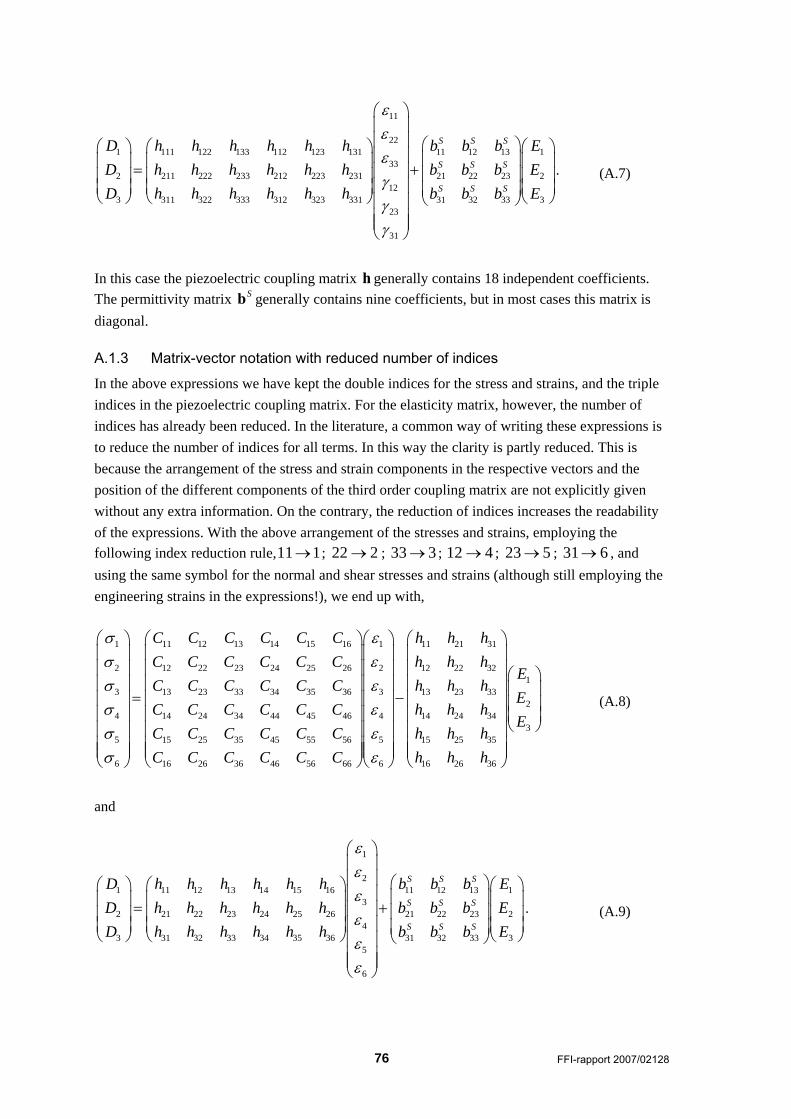
76 FFI-rapport 2007/02128
11
221 111 122 133 112 123 131 11 12 13 1
332 211 222 233 212 223 231 21 22 23 2
123 311 322 333 312 323 331 31 32 33 3
23
31
S S S
S S S
S S S
D h h h h h h b b b ED h h h h h h b b b ED h h h h h h b b b E
εεεγγγ
⎛ ⎞⎜ ⎟⎜ ⎟ ⎛ ⎞⎛ ⎞ ⎛ ⎞ ⎛ ⎞⎜ ⎟ ⎜ ⎟⎜ ⎟ ⎜ ⎟ ⎜ ⎟= +⎜ ⎟ ⎜ ⎟⎜ ⎟ ⎜ ⎟ ⎜ ⎟⎜ ⎟⎜ ⎟ ⎜ ⎟ ⎜ ⎟⎜ ⎟⎝ ⎠ ⎝ ⎠ ⎝ ⎠⎝ ⎠⎜ ⎟⎜ ⎟⎜ ⎟⎝ ⎠
. (A.7)
In this case the piezoelectric coupling matrix h generally contains 18 independent coefficients. The permittivity matrix Sb generally contains nine coefficients, but in most cases this matrix is diagonal.
A.1.3 Matrix-vector notation with reduced number of indices
In the above expressions we have kept the double indices for the stress and strains, and the triple indices in the piezoelectric coupling matrix. For the elasticity matrix, however, the number of indices has already been reduced. In the literature, a common way of writing these expressions is to reduce the number of indices for all terms. In this way the clarity is partly reduced. This is because the arrangement of the stress and strain components in the respective vectors and the position of the different components of the third order coupling matrix are not explicitly given without any extra information. On the contrary, the reduction of indices increases the readability of the expressions. With the above arrangement of the stresses and strains, employing the following index reduction rule,11 1→ ; 22 2→ ; 33 3→ ; 12 4→ ; 23 5→ ; 31 6→ , and using the same symbol for the normal and shear stresses and strains (although still employing the engineering strains in the expressions!), we end up with,
1 11 12 13 14 15 16 1 11 21
2 12 22 23 24 25 26 2
3 13 23 33 34 35 36 3
4 14 24 34 44 45 46 4
5 15 25 35 45 55 56 5
6 16 26 36 46 56 66 6
C C C C C C h hC C C C C CC C C C C CC C C C C CC C C C C CC C C C C C
σ εσ εσ εσ εσ εσ ε
⎛ ⎞ ⎛ ⎞⎛ ⎞⎜ ⎟ ⎜ ⎟⎜ ⎟⎜ ⎟ ⎜ ⎟⎜ ⎟⎜ ⎟ ⎜ ⎟⎜ ⎟
= −⎜ ⎟ ⎜ ⎟⎜ ⎟⎜ ⎟ ⎜ ⎟⎜ ⎟⎜ ⎟ ⎜ ⎟⎜ ⎟⎜ ⎟ ⎜ ⎟⎜ ⎟⎜ ⎟ ⎜ ⎟⎜ ⎟⎝ ⎠ ⎝ ⎠⎝ ⎠
31
12 22 321
13 23 332
14 24 343
15 25 35
16 26 36
hh h h
Eh h h
Eh h h
Eh h hh h h
⎛ ⎞⎜ ⎟⎜ ⎟⎛ ⎞⎜ ⎟⎜ ⎟⎜ ⎟⎜ ⎟⎜ ⎟⎜ ⎟
⎝ ⎠⎜ ⎟⎜ ⎟⎜ ⎟⎝ ⎠
(A.8)
and
1
21 11 12 13 14 15 16 11 12 13 1
32 21 22 23 24 25 26 21 22 23 2
43 31 32 33 34 35 36 31 32 33 3
5
6
S S S
S S S
S S S
D h h h h h h b b b ED h h h h h h b b b ED h h h h h h b b b E
εεεεεε
⎛ ⎞⎜ ⎟⎜ ⎟ ⎛ ⎞⎛ ⎞ ⎛ ⎞ ⎛ ⎞⎜ ⎟ ⎜ ⎟⎜ ⎟ ⎜ ⎟ ⎜ ⎟= +⎜ ⎟ ⎜ ⎟⎜ ⎟ ⎜ ⎟ ⎜ ⎟⎜ ⎟⎜ ⎟ ⎜ ⎟ ⎜ ⎟⎜ ⎟⎝ ⎠ ⎝ ⎠ ⎝ ⎠⎝ ⎠⎜ ⎟⎜ ⎟⎜ ⎟⎝ ⎠
. (A.9)

FFI-rapport 2007/02128 77
Remark that, for the piezoelectric coupling matrix the two latter indices are truncated into one. Once again we remark, that, in general, pq qph h≠ .
A.2 The strain-based constitutive law
From inverting the above expression, the strain-based constitutive laws in matrix-vector notation become
1 1 T− −= +ε C σ C h E (A.10) and
1 1( )T− −= + +D hC σ b hC h E . (A.11) These expressions are useful when converting the constitutive laws from a stress-based to a strain-based setting.
78 FFI-rapport 2007/02128
References
[1] APC International Ltd., Piezoelectric ceramics: principles and applications 2002.
[2] W. G. Cady, Piezoelectricity - an introduction to the theory and applications of electromechanical phenomena in crystals, Dover Publications, Inc., 1964.
[3] H. Jødahl, "Piezoelectric power supply for 30 mm programmable ammunition," Forsvarets forskningsinstitutt, FFI-rapport 2006/01865, 2006.
[4] F. Lorentzen and H. Jødahl, "Piezoelektrisk strømforsyning for engangsbruk," Forsvarets forskningsinstitutt,FFI-rapport 2003/00307, 2003.
[5] H. P. Langtangen, Computational partial differential equations - numerical methods and Diffpack programming, 2nd ed Springer-Verlag, 2003.
[6] "InuTech, www.diffpack.com," 2007.
[7] "MSC.Marc documentation, www.mscsoftware.com," 2007.
[8] S. Rahman, H. P. Langtangen, and C. H. W. Barnes, "A finite element method for modelling electromechanical wave propagation in anisotropic piezoelectric media," Communications in Computational Physics, vol. 2, no. 2, pp. 271-292, 2007.
[9] P. Gaudenzi and K.-J. Bathe, "An iterative finite element procedure for the analysis of piezoelectric continua," Journal of Intelligent Material Systems and Structures, vol. 6, pp. 266-273, 1995.
[10] C. T. Herakovich, Mechanics of fibrous composites, 1st ed John Wiley & Sons, Inc., 1998.
[11] J. Kim, V. V. Varadan, and V. K. Varadan, "Finite element modelling of structures including piezoelectric active devices," International Journal for Numerical Methods in Engineering, vol. 40, pp. 817-832, 1997.
[12] L. Costa, I. Figueiredo, R. Leal, P. Oliveira, and G. Stadler, "Modeling and numerical study of actuator and sensor effects for a laminated piezoelectric plate," Computers and Structures, vol. 85, pp. 385-403, 2007.
[13] C. K. Lee, "Theory of laminated piezoelectric plates for the design of distributed sensors/actuators. Part I: Governing equations and reciprocal relationships," Journal of the Acoustical Society of America, vol. 87, no. 3, pp. 1144-1158, 1990.
[14] M. Pozzi and T. King, "Piezoelectric modelling for an impact actuator," Mechatronics, vol. 13, pp. 553-570, 2003.
[15] J. Rödel, "Effective intrinsic linear properties of laminar piezoelectric composites and simple ferroelectric domain structures," Mechanics of Materials, vol. 39, pp. 302-325, 2007.
[16] R. D. Cook, D. S. Malkus, and M. E. Plesha, Concepts and applications of finite element analysis, 3rd ed John Wiley & Sons. Inc., 1989.

FFI-rapport 2007/02128 79
[17] T. Thorvaldsen, H. P. Langtangen, and H. Osnes, "Finite element modeling of elastic structures," in Advanced topics in computational partial differential equations- numerical methods and Diffpack programming. H. P. Langtangen and A. Tveito, Eds. Springer-Verlag, 2003, pp. 507-576.
[18] R. Bechmann, "Elastic and piezoelectric constants of alpha-quartz," Physical Review, vol. 110, no. 5, pp. 1060-1061, 1958.
[19] J. Yang, An introduction to the theory of piezoelectricity, 1st ed Springer-Verlag, 2005.
[20] B. P. Sorokin, P. P. Turchin, S. I. Burkov, D. A. Glushkov, and K. S. Aleksandrov, "Influence of static electric field, mechanical pressure and temperature on the propagation of acoustic waves in La_3Ga_5SiO_14 piezoelectric single crystals," 1996, pp. 161-169.
[21] A. W. Warner, M. Onoe, and G. A. Coquin, "Determination of elastic and piezoelectric constants for crystals in class (3m)," The Journal of the Acoustical Society of America, vol. 42, no. 6, pp. 1223-1231, 1967.
[22] H. Jaffe and D. A. Berlincourt, "Piezoelectric transducer materials," Proceedings of the IEEE, vol. 53, pp. 1372-1386, 1965.
[23] B. A. Auld, Acoustic fields and waves in solids John Wiley & Sons, Inc., 1973.
[24] B.D.Agarwal, L.J.Broutman, and K.Chandrashekhara, Analysis and performance of fiber composites, 3rd ed John Wiley & Sons, Inc., 2006.