tomas bata university in zlín - digilib.k.utb.cz
TRANSCRIPT

Tomas Bata University in Zlín Faculty of Applied Informatics
Dissertation Thesis for the degree of
Doctor of Sciences
The Evolutionary Computation Techniques in Chemical Engineering
Tran Trong Dao, Ing.
Supervisor: assoc. prof. Ivan Zelinka Study-branch: Technical Cybernetics
Zlín, Czech Republic, 2009

Acknowledgments:
Firstly, I would like to thank assoc. prof Ivan Zelinka for his helpful insights and discussions. Thank you, Ivan for the “green light” to go to the “world of evolutionary computation”, for supporting me from the beginning in a very professional way and being very kind and patient. Thank you for being a supervisor, a master and a big friend.
I would like to thank prof. Petr Dostál for his offer advise on model of chemical reactor and for precising this thesis.
Thanks to Dr. Zuzana Oplatková and Dr. Roman Šenkeřík for their helpful and advices at the Department of Applied Informatics during my study and research here, in Zlin.
I would also like to thank cordially my loving fiancée Le Thanh for the incredible moral support and love.
Thanks to all of my very kind and friendly friends, in the nice country of Czech Republic. I would just like to add that you know how great you are and that your support shall never be forgotten. Thank you very much.
Last, but not least, I'd like to thank my parents and “Mr. God“ for everything.

ABSTRACT
Chemical process control requires intelligent monitoring due to the dynamic nature of the chemical reactions and the non-linear functional relationship between the input and output variables involved. Chemical reactors is one of the major processing unit in many chemical, pharmaceutical and petroleum industries as well as in environmental and waste management engineering. In spite of continuing advances in optimal solution techniques for optimization and control problems, many of such problems remain too complex to be solved by the known techniques.
The main aim of this thesis is to show that such a powerful optimizing tool like evolutionary algorithms (EAs) can be in reality used for the optimization and predictive control of chemical processes. Four algorithms from the field of artificial intelligent - Differential evolution (DE), Self-organizing migrating algorithm (SOMA), Genetic algorithm (GA) and Simulated annealing (SA) are used in this investigation. In the first section EAs were used to investigative and optimize of batch reactor to improve its parameters. Consequently, EAs are used to model the technical requirements for chemical reaction. The second section presents the optimizing of chemical engineering processes, particularly those in which the evolutionary algorithm is used for static optimization and control of Continuous stirred tank reactors (CSTRs).
The optimizations and control chemical reactors have been performed in several ways, each one for a different set of reactor parameters or different cost function. The optimized and predictive control chemical reactor processes were used in simulations with optimization by evolutionary algorithms and the results are presented in graphs. Finally, experimental results are reported, followed by conclusion.
Keywords: Optimization, Simulation, Evolutionary Algorithms, Batch, CSTR.

RESUMÉ
Vzhledem k dynamice chemických reakcí a nelinearitě funkčních vztahů mezi vstupy a výstupy proměnných, vyžaduje řízení chemických procesů inteligentní kontrolu. „Chemický reaktor“ je jednou z hlavních procesních jednotek v chemickém, farmaceutickém a petrochemickém průmyslu, stejně jako v inženýrství řízení odpadu a životního prostředí. Navzdory pokračujícím pokrokům v rozvoji technik optimalizace a problémům řízení, stále existuje velká část příliš komplexních problémů, které se nedají řešit klasickými metodami.
Hlavním cílem této práce je demonstrovat fakt, že optimalizační nástroje, jakými jsou evoluční algoritmy (EA), mohou být použity pro prediktivní řízení a optimalizaci chemických procesů. V práci jsou použity čtyři algoritmy: Diferenciální evoluce (DE), Self organizing migrating algorithm (SOMA), Genetický algoritmus (GA) a Simulované žíhání (SA). V první části práce byly tyto evoluční algoritmy použity k optimalizaci parametrů dávkového reaktoru („batch reactor“). Následně jsou EA použity k modelování technických parametrů chemických reaktorů. Druhá část demonstruje optimalizaci chemických procesů, zvláště těch, ve kterých je použit evoluční algoritmus pro optimalizaci a řízení „Continuous stirred tank“ reaktorů.
Optimalizace a řízení chemických reaktorů byla provedena několika způsoby, každá pro jiný vektor parametrů reaktoru nebo s rozdílnou účelovou funkcí evolučního algoritmu. Veškeré optimalizované procesy jsou demonstrovány v grafech. Závěrem práce jsou prezentovány experimentální výsledky a jejich zhodnocení.
Klíčová slova: Optimalizace, Simulace, evoluční algoritmy, Batch, CSTR.

- 5 -
CONTENTS LIST OF FIGURES...........................................................................................................................7 LIST OF TABLES.............................................................................................................................9 LIST OF SYMBOLS AND ABBREVIATIONS..........................................................................11 1 INTRODUCTION .....................................................................................................................15 2 THE AIMS OF DISSERTATION............................................................................................17 3 CHEMICAL ENGINEERING PROCESS..............................................................................19
3.1 GENERAL INTRODUCTION..................................................................................................19 3.2 BATCH REACTOR ...............................................................................................................20
3.2.1 Characteristics of batch processes .....................................................................21 3.3 CONTINUOUS STIRRED TANK REACTORS (CSTR) ..............................................................22
3.3.1 Characteristics of CSTR process ........................................................................23 4 METHODS AND EVOLUTIONARY ALGORITHMS.........................................................25
4.1 INTRODUCTION AND A BRIEF SURVEY TO EVOLUTIONARY ALGORITHMS ..........................25 4.2 A BRIEF SURVEY OF SCOPING AND SCREENING CHEMICAL REACTION NETWORKS
USING STOCHASTIC OPTIMIZATION ....................................................................................30 4.3 SELECT EVOLUTIONARY ALGORITHMS .............................................................................33
4.3.1 Differential Evolution (DE) ................................................................................34 4.3.2 Self Organizing Migrating Algorithm (SOMA) ..................................................37 4.3.3 Genetic Algorithm (GA) .....................................................................................40 4.3.4 Simulated annealing (SA) ...................................................................................40
4.4 THE COST FUNCTION AND PRINCIPLE SIMULATION EVOLUTIONARY ALGORITHMS IN ENVIRONMENT MATHEMATICA .........................................................................................43 4.4.1 Quality of the evolutionary processes.................................................................47
5 SIMULATION PART – PROBLEM DESIGN AND EXPERIMENTAL RESULTS .........49 5.1 INTRODUCTION TO SIMULATION PART ...............................................................................49 5.2 THE MAIN AIM OF CHAPTER ...............................................................................................49 5.3 OPTIMIZATION OF BATCH REACTOR...................................................................................50
5.3.1 Description of batch reactor...............................................................................50 5.3.2 Problem design - Non-linear model of reactor...................................................52 5.3.3 Optimization of process parameters and the reactor geometry..........................53
5.3.3.1 Mathematical problems......................................................................54

- 6 -
5.3.3.2 The Cost Function (CF) .....................................................................55 5.3.3.3 Parameter settings ..............................................................................55 5.3.3.4 Experimental Results .........................................................................57 5.3.3.5 Discussion to the results optimization................................................70
5.3.4 Optimization of Continuous stirred tank reactor................................................72 5.3.4.1 Mathematical problems......................................................................72
5.3.5 Static optimization reactor .................................................................................74 5.3.5.1 The Cost Function (CF) .....................................................................74 5.3.5.2 Parameter settings ..............................................................................75 5.3.5.3 Experimental results...........................................................................76 5.3.5.4 Discussion and conclusion .................................................................86
6 PREDICTIVE CONTROL .......................................................................................................88 6.1 PRINCIPLE SIMULATION.....................................................................................................89 6.2 OPTIMIZATION OF CSTR VALUE WITH PREDICTION CONTROL...........................................90 6.3 RESULTS OF PREDICTIVE CONTROL....................................................................................91 6.4 DISCUSSION AND CONCLUSION TO THE RESULTS OF PREDICTIVE CONTROL .......................96
7 RESULTS OF DISSERTASION THESIS AND FURTHER RESEARCH PERSPECTIVE .........................................................................................................................97 7.1 EVALUATION OF THE OBJECTIVES......................................................................................97 7.2 GENERAL CONCLUSION AND FURTHER RESEARCH PERSPECTIVE........................................99
8 REFERENCES ........................................................................................................................101 LIST OF AUTHOR’S PUBLICATION ACTIVITIES..............................................................110 CURRICULUM VITAE ...............................................................................................................111

- 7 -
LIST OF FIGURES
Fig. 1. Batch reactor with single external cooling jacket ................................................. 22 Fig. 2. Scheme of Continuous Stirred Tank Reactor with Cooling Jacket ....................... 23 Fig. 3. The general scheme of an Evolutionary Algorithm in pseudo-code ...................... 26 Fig. 4. Structure of a single population evolutionary algorithm...................................... 27 Fig. 5. Structure of an extended multipopulation evolutionary algorithm........................ 27 Fig. 6. Population in the evolutionary algorithm.............................................................. 28 Fig. 7. Cost function surface representation, called Rana's function. .............................. 29 Fig. 8. Pseudo code of DE................................................................................................ 35 Fig. 9. Differential evolution, an artificial example
(http://www.icsi.berkeley.edu/~storn/code.html). ........................................... 36 Fig. 10. Pseudocode of SOMA ......................................................................................... 38 Fig. 11 . SOMA, an artificial example
(http://www.fai.utb.cz/people/zelinka/soma)................................................... 39 Fig. 12. Pseudocode of GA (http://www.ra.cs.uni-
tuebingen.de/software/EvA2/)......................................................................... 40 Fig. 13. Structure of simulated annealing algorithm ........................................................ 42 Fig. 14. Principle simulation evolutionary algorithms ..................................................... 45 Fig. 15. General subroutines call of SOMA, DE, GA, SA in environment
Mathematica ................................................................................................... 46 Fig. 16. Overview process “Start EA” in environment Mathematica (1x
simulation of version SOMAATO) .................................................................. 47 Fig. 17. Scheme Batch reactor .......................................................................................... 51 Fig. 18. Parameter variation of SOMA and DE................................................................ 61 Fig. 19. Parameter variation of GA and SA...................................................................... 62 Fig. 20. Process parameters for 100 simulations of SOMA - version
SOMAATO ...................................................................................................... 63 Fig. 21. Process parameters for 100 simulations of SOMA - version
SOMAATR....................................................................................................... 64 Fig. 22. Process parameters for 100 simulations of DE - version DERan1Bin................ 65 Fig. 23. Process parameters for 100 simulations of DE - version DERan2Bin................ 66

- 8 -
Fig. 24. Process parameters for 100 simulations of GA ................................................... 67 Fig. 25. Process parameters for 100 simulations of SA – version SA_Elitism.................. 68 Fig. 26. Process parameters for 100 simulations of SA – version SA_NoElitism ............. 69 Fig. 27. 100 simulations for T ........................................................................................... 71 Fig. 28. Continuous Stirred Tank reactor ......................................................................... 72 Fig. 29. Parameter variation of SOMA and DE for model CSTR ..................................... 80 Fig. 30. Parameter variation of SA and GA for model CSTR ........................................... 81 Fig. 31. Process parameters of cA for 100 simulations of each algorithm...................... 82 Fig. 32. Process parameters of cB for 100 simulations of each algorithm...................... 83 Fig. 33. Process parameters of Tr for 100 simulations of each algorithm...................... 84 Fig. 34. Process parameters of Tc for 100 simulations of each algorithm....................... 85 Fig. 35. Best solution of SOMA........................................................................................ 87 Fig. 36. Principle of predictive control by evolutionary algorithm .................................. 88 Fig. 37. Principle simulation............................................................................................. 90 Fig. 38. Predictive control temperatures Tr and Tc of CSTR by SOMAATO,
“red” was required value .............................................................................. 92 Fig. 39. Predictive control temperatures Tr and Tc of CSTR by DERan1Bin,
“red” was required value .............................................................................. 93 Fig. 40. Predictive control temperatures Tr and Tc of CSTR by GA, “red” was
required value ................................................................................................. 94 Fig. 41. Predictive control temperatures Tr and Tc of CSTR by SA_Elitism,
“red” was required value .............................................................................. 95

- 9 -
LIST OF TABLES
Tab.1 Parameters of reactor, “yellow” was optimized..................................................... 53 Tab.2 SOMA parameter setting........................................................................................ 55 Tab.3 DE parameter setting .............................................................................................. 56 Tab.4 GA parameter setting .............................................................................................. 56 Tab.5 SA parameter setting ............................................................................................... 56 Tab.6 Optimized reactor parameters and their range inside which has been
optimization done............................................................................................ 57 Tab.7 The best values of optimized parameters by SOMA, DE......................................... 58 Tab.8 The best values of optimized parameters by GA, SA............................................... 58 Tab.9 Estimated parameters for DERand1Bin.................................................................. 58 Tab.10 Estimated parameters for DERand2Bin................................................................ 59 Tab.11 Estimated parameters for SOMAATO................................................................... 59 Tab.12 Estimated parameters for SOMAATR ................................................................... 59 Tab.13 Estimated parameters for GA................................................................................ 60 Tab.14 Estimated parameters for SA_Elitism ................................................................... 60 Tab.15 Estimated parameters for SA_NoElitism............................................................... 60 Tab. 16 Parameters, inlet values and initial conditions.................................................... 73 Tab. 17. Parameters of reactor, “yellow” was optimized................................................. 74 Tab.18 SOMA parameter setting for simulation of CSTR model ...................................... 75 Tab.19 Optimized reactor parameters and their range inside which has been
optimization done............................................................................................ 75 Tab. 20. The best values of optimized parameters by SOMA, DE..................................... 76 Tab. 21. The best values of optimized parameters by GA, SA........................................... 76 Tab.22 Estimated parameters of version SOMAATO........................................................ 77 Tab.23 Estimated parameters of version SOMAATR ........................................................ 77 Tab.24 Estimated parameters of version DERan1Bin....................................................... 77 Tab.25 Estimated parameters of version DERan2Bin....................................................... 78 Tab.26 Estimated parameters of version GA .................................................................... 78 Tab.27 Estimated parameters of version SA_Elitism ........................................................ 78

- 10 -
Tab.28 Estimated parameters of version SA_NoElitism ................................................... 79 Tab. 29 Range inside for predictive control of CSTR........................................................ 91 Tab. 30. Parameters setting for predictive control of CSTR............................................. 91

- 11 -
LIST OF SYMBOLS AND ABBREVIATIONS
symbol unit meaning
EAs - evolutionary algorithms EA - evolutionary algorithm DE - differential evolution SOMA - self-organizing migrating algorithm GA - genetic algorithm SA - simulated annealing CSTRs - continuous stirred tank reactors EP - evolutionary programming ES - evolution Strategies AGO - algorithms global optimization xi,G - individual in the current generation x’i,G - DE generates a new trial individual xr1,G, xr2,G - randomly selected individuals ui,G+1 - perturbation vector G - current generation δ - a random number ΔE - the newly generated solution
FKm& [kg.s-1] mass flow rate of ”Input Chemical FK”
FKT [K] temperature of ”Input Chemical FK”
FKc [J.kg. K-1] specific heat of ”Input Chemical FK”
Vm& [kg.s-1] mass flow rate of “Input cooling medium”
VPT [K] temperature of “Input cooling medium”
VRm [kg] total weigh of jacketed through space of reaction
VT [K] temperature of “output cooling medium”

- 12 -
Vc [J.kg. K-1] specific heat of “output cooling medium”
Pm [kg] parameter mass initial batch inside the reactor
m [kg] total mass of reactionary mixture T [K] temperature of reactionary mixture
Rc [J.kg. K-1] specific heat of reactionary mixture
FKa [kmol m-3] concentration of chemical FK A [s-1] frequency factor ρP [kg.m-3] density of chemical P K [kg. s-3. K-1] coefficient of heat transfer ρFK [kg.m-3] density of chemical FK r [m] diameter of vessel h [m] weight of vessel ΔHr [J. kg-1] heat of reaction
tfcos - cost function PathLength - Control parameter of SOMA; it
determines the stopping position of the movement of an individual
F - mutation constant CR - constant of crossover NP - number individuals of population in
DE Step - step size of migration PRT - perturbation constant PopSize - population size in SOMA Migrations - number of rounds of migrations in
SOMA MinDiv - max. division values cost function of
individuals sufficient for stopping algorithms
Individual Length - length of individuals MutationCostant - mutation constant Generations - number of generation cycles in DE PocetCastic - number particle

- 13 -
DERan1Bin - strategy random version 1 Bin for DE
DERan2Bin - strategy random version 2 Bin for DE
SOMAATO - SOMA All to One SOMAATR - SOMA All to One Random SA_Elitism - strategy SA with Elitism SA_NoElitism - strategy SA without Elitism Vr [m3] volume of the reactant mixture Vc [m3] volume of the coolant Qr [m3min-1] volumetric flow rate of the reactant
mixture Qc [m3min-1] volumetric flow rate of the coolant ρr [kg m-3] density of the ρc [kg m-3] density of the the coolant cpr [kJ kg-1K-1] specific heat capacity of the reactant
mixture cpc [kJ kg-1K-1] specific heat capacity of the coolant Ar [m2] heat exchange surface area U [kJ m-2min-1K-1] heat transfer coefficient k10, k20 [m-1] pre-exponential factors
E1, E2 [K J Kkmol−1] activation energies
R [J K mol−1] gas constant h1, h2 [kJ kmol-1] reaction enthalpies cAi [kmol m-3] concentration of chemical A for feed
(inlet) value cBi [kmol m-3] concentration of chemical B for feed
(inlet) value Tri [K] temperature of the reactant mixture
(inlet) Tci [K] concentration of the coolant (inlet) cA
s [kmol m-3] concentration of chemical A for
steady-state value cB
s [kmol m-3] concentration of chemical B for
steady-state value

- 14 -
Trs [K] temperature of the reactant for
steady-state value Tc
s [K] temperature of the coolant for
steady-state value
- 15 -
1 INTRODUCTION
The optimization of dynamic process has received growing attention in recent years because it is essential for the process industry to strive for more efficient and agile manufacturing in face of saturated market and global competition (T. Backx, O. Bosgra 2000).
Evolutionary algorithms such as evolution strategies and genetic algorithms have become the method of choice for optimization problems that are too complex to be solved using deterministic techniques such as linear programming or gradient (Jacobian) methods. The large number of applications (Beasley (1997)) and the continuously growing interest in this field are due to several advantages of EAs compared to gradient based methods for complex problems (Ivo F. Sbalzarini, Sibylle Muller and Petros Koumoutsakos 2000).
In chemical engineering, evolutionary optimization has been applied by the author and others to system identification (Pham and Coulter, 1995; Moros, 1996); a model of a process is built and its numerical parameters are found by error minimization against experimental data. Evolutionary optimization has been widely applied to the evolution of neural networks models for use in control applications (e.g. Li & Haubler, 1996).
The area of reactor network synthesis currently enjoys a proliferation of contributions in which researchers from various perspectives are making efforts to develop systematic optimization tools to improve the performance of chemical reactors. The contributions reflect on the increasing awareness that textbook knowledge and heuristics (Levenspiel, 1962), commonly employed in the development of chemical reactors, are now deemed responsible for the lack of innovation, quality, and efficiency that characterizes many industrial designs.
The main aim of this participation is to show that evolutionary algorithms (EAs) are capable of optimization on chemical engineering processes. The ability of EAs to successfully work with at investigation on optimization and predictive control of chemical reactors.

- 16 -
Firstly, a non-linear mathematical model is required to describe the dynamic behaviour of batch process; this justifies the use of evolutionary method of the EAs to deal with this process, for static optimization of a chemical batch reactor. Consequently, it is used to design geometry technique equipments for chemical reaction. The method was used to optimize the design of the growth chamber, and was found to be in good agreement with the observed growth rate results. The second one was chosen for optimization of a continuous stirred tank reactor (CSTR). On the next part, we have used EAs to predictive control of chemical process of rectors too.
The following and the biggest part describes the results of optimization of chemical process. The optimizations and control chemical reactors have been performed in several ways, each one for a different set of reactor parameters or different cost function. The optimized reactor and predictive control were used in a simulation with optimization by evolutionary algorithms and the results are presented in graphs.
This thesis is followed by a brief description of the chemical reactors and used EAs. Evolutionary algorithms are then studied, and finally experimental results are reported, followed by conclusion.

- 17 -
2 THE AIMS OF DISSERTATION
This dissertation aims to show how methods of artificial intelligence--mainly evolutionary computational techniques--can be used in dynamical systems of chemical reactors, particularly for the complex tasks of analyses and optimization of predictive control. The main focus here is on the examples of evolution algorithms (EAs) implementation in methods for achieving stable chemical reaction. The purpose is to obtain better results, meaning efficiency in reaching the desired stable state and superior stabilisation, through having robust and effective optimization of predictive control.
EAs is used to determine the optimal settings for the adjustable parameters, which are then used to achieve the desired state or behaviour of the chemical reactors' process. As noted in the results and conclusion of the presented project, EAs are able to find the optimal solution for the selected control technique. Thus avoiding complicated mathematical analysis of chemical process to find the settings for control method.
Research on this thesis is concerned with the field of optimization of chemical engineering through EAs. The main purposes and goals of the research can be summarised as thus:
1. Introduction of the chemical engineering process, formulation of the mathematical problems, and the description and analysis of the chosen dynamic systems--more concretely those in the processes of a Batch reactor and a Continuous stirred-tank reactor (CSTR);
2. Proposing a set of solving algorithms for the application of stochastic optimization, which enhances confidence in the optimization results, particularly in the chemical reaction;
3. Selecting and demonstrating EAs and practical method to optimize the chemical process, especially of Batch and CSTR reactors;

- 18 -
4. Demonstrating the use of designed algorithms for global optimization of the predictive control chemical processes and comparison between each selected algorithms; and
5. Presenting conclusions and suggesting further research perspective.

- 19 -
3 CHEMICAL ENGINEERING PROCESS
3.1 General introduction The chemical industry produces many products by using chemical reaction
and physical processes. To successfully realize these processes of chemical technology, it is necessary to make quantitative and qualitative analyses, especially in places where there is planned automated systems of technology processes control. To make the modernization of present and future processes purposeful, it is necessary to divide the modernization into periods.
The first and very important period is the analyzing of the industrial producing system. It usually includes simulations based on real model of chemical-physical processes for converting input sources into output products. These simulations will show the important key points of the technological process and where necessary changes to a new control system will be able to significantly improve the technological process’s efficiency.
It is possible to say generally that the key technological points are the chemical reactors. To design the optimal parameters of reactor and its control system is one of the most difficult tasks of the process engineering. The situation is very often complicated by the imprecise kinetic principles of chemical reaction, which necessitates extensive measurements of dependencies of input and output elements on time, temperature, pressure, and etc. These quite complicated kinetic models (which are usually verified by experimental measurements) can be simplified using different methods into simpler models of which known methods of control already exist.
Notwithstanding the petrochemical industry, big attention must be paid to materials used in the production of macromolecular substances, i.e. plastic materials. Macromolecular substances are created from two kinds of reactions – polymerization and polycondensation. Algorithms must be designed to control these reactions, of which the majority comprises exothermic reactions (they produce heat). From an economic point of view, it is expected to have maximum efficiency of chemical reactor productivity with required quality. The reactor productivity depends on reacting speed, and reacting speed usually rises exponentially with temperature.

- 20 -
Although it may seem that the exothermal kind of reaction is a big advantage for us, it may not always be true due to security reasons and product quality (rising temperature may decrease the output product quality). The product quality may decrease especially in cases when the main reaction is followed by side reactions, their speed exponentially raised with temperature as well. As such, the most important parameter that has to be controlled during exothermic reactions is the reaction compound temperature. For this reason, the models presented in this work are based on enthalpy balances, with relevant simulations.
Nowadays, the application domain of chemical reactions and reactors constitutes one of the backbones for interdisciplinary collaboration. In fact, the optimization of industrial chemical processes has drawn attention in recent years. For experimental determination of the most important parameter - this thesis is described and analysed process of a Batch and Continuous stirred tank reactors. It is hoped that the examples presented here will provide some appreciation of the creative process.
3.2 Batch reactor The Batch reactor is the generic term for a type of vessel widely used
in the process industries. Its name is something of a misnomer since vessels of this type are used for a variety of process operations such as solids dissolution, product mixing, chemical reactions, batch distillation, crystallization, liquid/liquid extraction and polymerization. In some cases, they are not referred to as reactors but have a name which reflects the role they perform (such as crystallizer, or bio reactor).
The advantages of the batch reactor lie with its versatility. A single vessel can carry out a sequence of different operations without the need to break containment. This is particularly useful when processing, toxic or highly potent compounds.

- 21 -
3.2.1 Characteristics of batch processes
The optimization of batch processes has attracted attention in recent years (Aziz et al. 2000; Silva et al. 2003) because, in the face of growing competition, it is a natural choice for reducing production costs, improving product quality, meeting safety requirements and environmental regulations. Batch and semi-batch processes are of considerable importance in the fine chemicals industry. A wide variety of special chemicals, pharmaceutical products, and certain types of polymers are manufactured in batch operations. Batch processes are typically used when the production volumes are low, when isolation is required for reasons of sterility or safety, and when the materials involved are difficult to handle. In batch operations, all the reactants are charged in a tank initially and processed according to a pre-determined course of action during which no material is added or removed. In semi-batch operations, a reactant may be added with no product removal, or a product may be removed with no reactant addition, or a combination of both. From a process systems point of view, the key feature that differentiates continuous processes from batch and semi-batch processes is that continuous processes have a steady state, whereas batch and semi-batch processes do not (Srinisavan 2000 et al. 2002a and 2000b).
Reactor Configurations
In batch system all reactants are added to the tank at the given starting time. During the course of reaction, the reactant concentrations decrease continuously with time, and products are formed. On completion of the reaction, the rector is emptied, cleaned and is made ready for another batch.
This type of operation provides great flexibility with very simple equipment and allows differing reaction to be carried out in the same reactor. The disadvantages are the downtime needed for loading and cleaning and possibly the changing reaction conditions. Batch operation is often ideal for small scale flexible production and high value, low output product production, where the chemistry and reaction kinetics are not known exactly. In semi-batch operation, one reactant may be charged to the vessel at the start of the batch, and then the other fed to the reactor at perhaps varying rate and over

- 22 -
differing time periods. When the vessel is full, feeding is stopped and the contents allowed to discharge. Semi-batch operation allows one to vary the reactant concentration to a desired level in a very flexible way, and thus to control the reaction rates and the reactor temperature. It is, however, necessary to develop an appropriate feeding strategy. Modelling and simulation allows estimation of optimal feeding profiles. Sometimes it is necessary to adjust the feeding rates using feedback control. The flexibility of operation is generally similar to that of a batch reactor system. (J. Ingham, I.J.Dunn, E.Heinzle, J.E.P 2000).
Heat transfer to and from reactor
Heat transfer is usually affected by coils or jackets, but can also be achieved with the use of external loop heat exchanger and, in certain case; heat is transported out of the reactor. The treatment here mainly concerns jackets and coils.
Fig. 1. Batch reactor with single external cooling jacket
3.3 Continuous stirred tank reactors (CSTR) The continuous stirred-tank reactor (CSTR), also known as vat- or back
mix reactor is a common ideal reactor type in chemical engineering. A CSTR

- 23 -
often refers to a model used to estimate the key unit operation variables when using a continuous agitated-tank reactor to reach a specified output.
CSTR runs at steady state with continuous flow of reactants and products; the feed assumes a uniform composition throughout the reactor, exit stream has the same composition as in the tank.
Fig. 2. Scheme of Continuous Stirred Tank Reactor with Cooling Jacket
where A is the raw material, B is the desired product, and C is an undesired by-product.
3.3.1 Characteristics of CSTR process
Continuous stirred tank reactors (CSTRs) belong to a class of nonlinear systems where both steady-state and dynamic behaviour are nonlinear. Their models are derived and described in e.g. (Ogunnaike and Ray, 1994), (Schmidt, 2005) and (Corriou, 2004). verification can be found in (Stericker and Sinha, 1993).
Chemical process control requires intelligent monitoring due to the dynamic nature of the chemical reactions and the non-linear functional relationship between he input and output variables involved. CSTR is one of

- 24 -
the major processing unit in many chemical, pharmaceutical and petroleum industries as well as in environmental and waste management engineering. In spite of continuing advances in optimal solution techniques for optimization and control problems, many of such problems remain too complex to be solved by the known techniques (Emuoyibofarhe O.Justice, Reju A Sunday, 2008).

- 25 -
4 METHODS AND EVOLUTIONARY
ALGORITHMS
4.1 Introduction and a brief survey to Evolutionary Algorithms
As the history of the field suggests there are many different variants of Evolutionary Algorithms. The common underlying idea behind all these techniques is the same: given a population of individuals the environmental pressure causes natural selection (survival of the fittest) and this causes a rise in the fitness of the population. Given a quality function to be maximised we can randomly create a set of candidate solutions, i.e., elements of the function’s domain, and apply the quality function as an abstract fitness measure – the higher the better. Based on this fitness, some of the better candidates are chosen to seed the next generation by applying recombination and/or mutation to them. Recombination is an operator applied to two or more selected candidates (the so-called parents) and results one or more new candidates (the children). Mutation is applied to one candidate and results in one new candidate. Executing recombination and mutation leads to a set of new candidates (the offspring) that compete – based on their fitness (and possibly age)– with the old ones for a place in the next generation. This process can be iterated until a candidate with sufficient quality (a solution) is found or a previously set computational limit is reached. In this process there are two fundamental forces that form the basis of evolutionary systems.
Variation operators (recombination and mutation) create the necessary diversity and thereby facilitate novelty, while Selection acts as a force pushing quality.
The combined application of variation and selection generally leads to improving fitness values in consecutive populations. It is easy (although some-what misleading) to see such a process as if the evolution is optimising, or at least “approximising”, by approaching optimal values closer and closer over its course. Alternatively, evolution it is often seen as a process of adaptation. From this perspective, the fitness is not seen as an objective function to be optimised, but as an expression of environmental requirements. Matching

- 26 -
these requirements more closely implies an increased viability, reflected in a higher number of offspring. The evolutionary process makes the population adapt to the environment better and better.
Let us note that many components of such an evolutionary process are stochastic. During selection fitter individuals have a higher chance to be selected than less fit ones, but typically even the weak individuals have a chance to become a parent or to survive. For recombination of individuals the choice of which pieces will be recombined is random. Similarly for mutation, the pieces that will be mutated within a candidate solution, and the new pieces replacing them, are chosen randomly. The general scheme of an Evolutionary Algorithm can is given in Fig. 3 in a pseudo-code fashion. (A.e. Eiben and j.e. Smith, 2003).
BEGIN
INITIALISE population with random candidate solutions;
EVALUATE each candidate;
REPEAT UNTIL ( TERMINATION CONDITION is satisfied ) DO
1 SELECT parents;
2 RECOMBINE pairs of parents;
3 MUTATE the resulting offspring;
4 EVALUATE new candidates;
5 SELECT individuals for the next generation;
OD
END
Fig. 3. The general scheme of an Evolutionary Algorithm in pseudo-code
Structure of a population evolutionary algorithm show in Fig. 4. & 5.

- 27 -
Fig. 4. Structure of a single population evolutionary algorithm
Fig. 5. Structure of an extended multipopulation evolutionary algorithm
Overview from source: http://www.geatbx.com/docu/algindex-01.html
start
are optimization criteria met?
Initialization • Creation of
initial population • Evaluation of
individuals
best individuals
Fitness assignment selection
recombination
mutation
Generate new
population
yes
Evaluation of offspring
reinsertion
migration
competition
no
yes
are optimization criteria met?
generate initial
population evaluative objective
functionbest
individuals
start selection
recombination
mutation
Generate new
population
yes
no
- 28 -
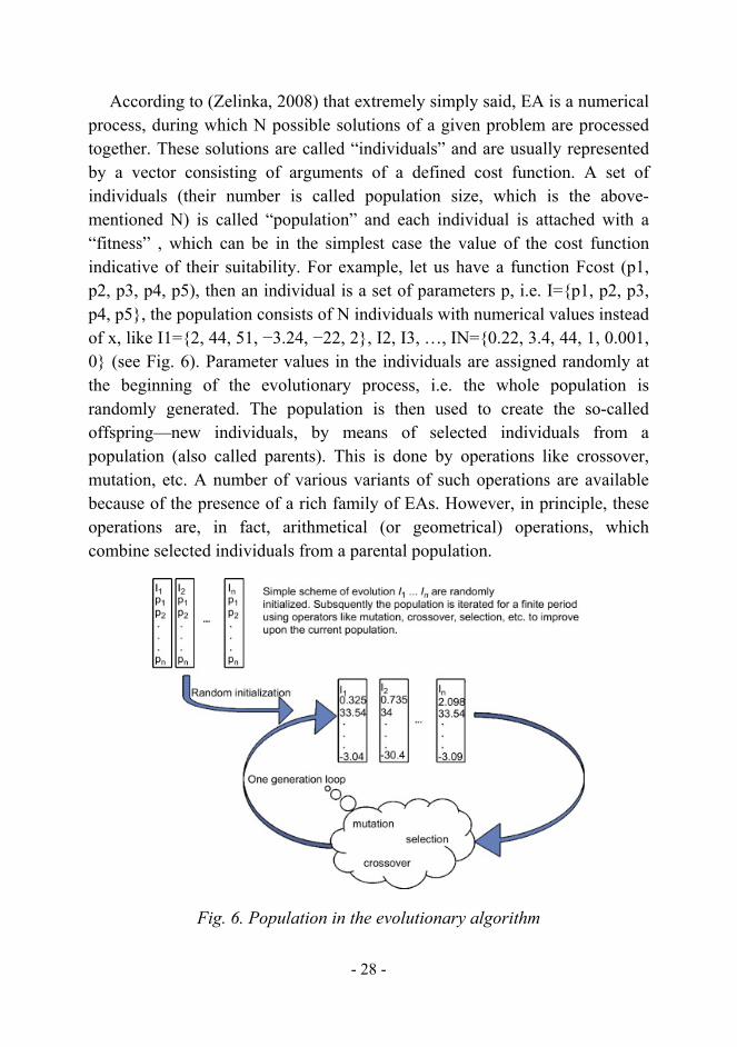
According to (Zelinka, 2008) that extremely simply said, EA is a numerical process, during which N possible solutions of a given problem are processed together. These solutions are called “individuals” and are usually represented by a vector consisting of arguments of a defined cost function. A set of individuals (their number is called population size, which is the above-mentioned N) is called “population” and each individual is attached with a “fitness” , which can be in the simplest case the value of the cost function indicative of their suitability. For example, let us have a function Fcost (p1, p2, p3, p4, p5), then an individual is a set of parameters p, i.e. I={p1, p2, p3, p4, p5}, the population consists of N individuals with numerical values instead of x, like I1={2, 44, 51, −3.24, −22, 2}, I2, I3, …, IN={0.22, 3.4, 44, 1, 0.001, 0} (see Fig. 6). Parameter values in the individuals are assigned randomly at the beginning of the evolutionary process, i.e. the whole population is randomly generated. The population is then used to create the so-called offspring—new individuals, by means of selected individuals from a population (also called parents). This is done by operations like crossover, mutation, etc. A number of various variants of such operations are available because of the presence of a rich family of EAs. However, in principle, these operations are, in fact, arithmetical (or geometrical) operations, which combine selected individuals from a parental population.
Fig. 6. Population in the evolutionary algorithm

- 29 -
Evolutionary process is thus an iterative process with the selection and survival of the temporarily best solutions, which are used in the next generation to create better solutions.
Finally, the best individual (i.e. problem solution) is selected from the last population and is regarded like the best solution from the actually ended evolution. The cost function used in the population should be defined so that its minimization or maximization should lead to the optimal solution. From this point of view, evolution can be also regarded like a mutually parallel search of an N-dimensional, nonlinear and complicated surface, where each point represent a possible solution. Example of the “cost function landscape” of the individual with two parameters, I={x, y} is depicted in Fig. 7 (see also Zelinka, 2004). Cost value is on the axis “z”.
Fig. 7. Cost function surface representation, called Rana's function.
Today, a rich set of various versions of EAs exists. They differ by mathematical principles driving their evolutionary process as well as by the
- 30 -
fundamentally unique terminology and algorithm philosophy employed. Another difference is also that of individual representation, i.e. an individual can consist of integer or/and real numbers like I={2, 44, 51, −3.24, −22, 2} or can be based on binary string I={0010101101010101}, which is typical for genetic algorithm (GA) in its canonical version.
For a closer and more detailed study of EAs, which is time-consuming, it is recommended to use the literature like, for example, Holland (1975) and Davis (1996) (GAs), (Price, 1994), (Price, 1996) and (Price, 1999) (differential evolution (DE)), Kirkpatrick et al. (1983) and Cerny (1985) (simulated annealing (SA)), Eberhart and Kennedy (1995) and Clerc (2006) (particle swarm), Zelinka, (2004) (self-organizing migrating algorithm (SOMA)), Beyer (2001) (evolutionary strategies (ES)), Dorigo and Stützle (2004) (ant colony optimization), or in general Back et al. (1997).
4.2 A brief survey of Scoping and Screening chemical reaction networks using stochastic optimization
Many methods were adapted for the so-called optimal chemical reactors. The new methods focus on a systematic and thorough consideration of the available options and employ technology in the form of superstructures, optimization techniques, and a variety of graphical methods.
The importance of mathematical methods in optimizing reactors has been exemplified early enough with the application of dynamic programming for the estimation of optimal operating conditions in CSTR cascades (Aris, 1960) and the development of graphical techniques for single reversible reactions in PFRs (1961).
Around the same time, a set of brilliant contributions by Horn (1964) provided the basis of material that later emerged as attainable-region (AR) approaches. Dyson and Horn (1967) developed graphical tools for optimal temperature control schemes, feed distribution profiles along a PFR and catalyst minimization problems (Dyson and Horn, 1969). In these early days, separate groups made attempts to consolidate options and alternatives within comprehensive reactor structures (Ng and Rippin, 1965; Jackson, 1968;

- 31 -
Ravimohan, 1971). Optimization approaches initially addressed fixed reactor structures. Examples include the work of Paynter and Haskins (1970), and Chitra and Govind (1981, 1985a,b). The first studies of comprehensive structures should be attributed to Achenie and Biegler (1986, 1988, 1990), who employed existing representations (Jackson, 1968; Ng and Rippin, 1965) to launch optimization techniques in the form of NLP methods.
Kokossis and Floudas (1990, 1991, 1994) first introduced the idea of a reactor network superstructure modeled and optimized as an MINLP formulation. Though general and inclusive, their representation did not follow previous developments, but made an effort to facilitate the functionalities of the MINLP technology with the synthesis objectives. Mainly to scope, optimize and analyze the reaction process, Kokossis and Floudas replaced detailed models with simple though generic structures, enough to screen for design options and estimate the limiting performance of the reaction system. In the same vane, dynamic components have been replaced by CSTR cascades. A superstructure of generic elements (ideal CSTRs and PFRs) was postulated to account for all possible interconnections among the units. The representation was modeled and optimized as a MINLP model.
Though fundamental limitations appear evident, persistent efforts to extend the graphical methods have appeared in the literature (Hildebrandt et al., 1990; Hildebrandt and Glasser, 1990; Glasser et al., 1992, 1994; Feinberg and Hildebrandt, 1997; Price et al., 1997; Glasser and Hildebrandt, 1997; Hopley et al., 1996; Nisoli et al., 1997; McGregor et al., 1999; Godorr et al., 1999.)
A more promising direction has been pursued by Biegler and coworkers. The motivation has been to instill better guarantees in the optimization efforts by exploiting ideas and rules established in the construction of the AR. Applications presented in this area include the work by Balakrishna and Biegler (1992a,b) and Lakshmanan and Biegler (1994, 1996, 1997), and involved mathematical programming applications in the form of NLP and MINLP formulations. Optimal control formulation has been presented by Rojnuckarin et al. (1996) and Schweiger and Floudas (1999). Hildebrandt and Biegler (1994) presented a review of the attainable region approaches and suggested areas for future development of the concept. (Marcoulaki and Kokossis, 2004).

- 32 -
Especially in recent years, the methods of artificial intelligence, namely the evolutionary algorithms were used to optimise successfully chemical processes.
The optimization of non-linear constrained problems is relevant to chemical engineering practice [Wong, (1990); Salcedo, (1992); Floudas, (1995)]. Nonlinearities are introduced by process equipment design relations, by equilibrium relations and by combined heat and mass balances. The design variables may be floating points [non-linear programming (NLP) problems] or some of them may be integers [mixed integer non-linear programming (MINLP) problems].
In recent years, evolutionary algorithms (EAs) have been applied to the solution of NLP in many engineering applications. The best-known algorithms in this class include Genetic Algorithms (GA), Evolutionary Programming (EP), Evolution Strategies (ES) and Genetic Programming (GP). There are many hybrid systems, which incorporate various features of the above paradigms and consequently are hard to classify, which can be referred just as EC methods Dasgupta and Michalewicz, (1997). They differ from the conventional algorithms since, in general, only the information regarding the objective function is required. In recent years, EC methods have been applied to a broad range of activities in process system engineering including modeling, optimization and control. See for example real-time control of plasma reactor (Nolle et al., 2001 and (Nolle et al., 2005); Zelinka and Nolle, 2006), Optimization and control of batch reactor by evolutionary algorithms Senkerik, Zelinka, 2005], Optimization of reactive distillation processes using Self-organizing Migrating Algorithm and Differential Evolution Strategies (Tran, Zelinka, 2008), Using method of artificial intelligence to optimise and control chemical reactor (Tran, Zelinka, 2009), Investigation on optimization of Process Parameters and chemical reactor geometry by evolutionary algorithms (Tran, Zelinka, 2009) or An optimum solution for a process control problem (continuous stirred tank reactor) using a hybrid neural network (Emuoyibofarhe O.Justice, Reju A Sunday, 2008)…

- 33 -
4.3 Select Evolutionary Algorithms For the experiments described here, stochastic optimisation algorithms,
such as Differential Evolution (DE) (Price, 1999), Self-Organizing Migrating Algorithm (SOMA) (Zelinka, 2004), Genetic Algorithms (GA) (Holland, 1975) and Simulated Annealing (SA) (Kirkpatrick et al., 1983; Cerny, 1985) were selected. Main reason why DE, SOMA, GA and SA have been seed comes from contemporary state in chemical engineering and EAs use. Since now has been done some research with attention on use of EAs in chemical engineering optimization, including DE. This participation has to show that applicability of relatively new algorithms is also positive and can lead to applicable results, as was shown for example in Zelinka (2001), which has been done under 5th EU project RESTORM (acronym of Radically Environmentally Sustainable Tannery Operation by Resource Management) and main aim was to use EAs in chemical engineering processes. True is also that there is a plenty of other heuristic like particle swarm (Liu, Liu, Cartres, 2007), scatter search (Glover, Laguna, Martí, 2003), memetic algorithms, simulated annealing (Kirkpatrick, Gelatt, Vecchi, 1983), etc. and according to No Free Lunch teorem (Wolpert, Macready, 1997) is clear that each heuristic would be less or more applicable on example presented here. SOMA is a stochastic optimization algorithm that is modelled on the social behaviour of co-operating individuals (Zelinka, 2004). It was chosen because it has been proved that the algorithm has the ability to converge towards the global optimum (Zelinka, 2004). GA is one of the most modern paradigms for general problem solving. Genetic algorithms are more robust than existing directed search methods. Another important property of GA based search methods is that they maintain population of potential solutions – all other methods process a single point of the search space like hill climbing method. Hill climbing methods provide local optimum values and these values depend on the selection of starting point. Also there is no information available on the relative error with respect to global optimum. To increase the success rate in hill climbing method, it is executed for large number of randomly selected different starting points. On the other hand, GA is a multi-directional search maintaining a population of potential solutions and encourages information formation and exchange between these directions. Furthermore, SA is a generic probabilistic meta-algorithm for the global optimization problem,

- 34 -
namely locating a good approximation to the global optimum of a given function in a large search space. SA has been used in various combinatorial optimization problems and has been particularly successful in circuit design problems (see Kirkpatrick et al. 1983).
4.3.1 Differential Evolution (DE)
Differential Evolution (Price, 1999) (see Fig. 9) is a population-based optimization method that works on real-number coded individuals. For each individual xi,G in the current generation G, DE generates a new trial individual x’i,G by adding the weighted difference between two randomly selected individuals xr1,G and xr2,G to a third randomly selected individual xr3,G. The resulting individual x’i,G is crossed-over with the original individual xi,G. The fitness of the resulting individual, referred to as perturbated vector ui,G+1, is then compared with the fitness of xi,G. If the fitness of ui,G+1 is greater than the fitness of xi,G, xi,G is replaced with ui,G+1, otherwise xi,G remains in the population as xi,G+1. Deferential Evolution is robust, fast, and effective with global optimization ability. It does not require that the objective function is differentiable, and it works with noisy, epistatic and time-dependent objective functions. Pseudocode of DE shows:

- 35 -
( ) ( ) ( )
[ ] ( )
⎪⎪⎪⎪⎪⎪⎪⎪
⎩
⎪⎪⎪⎪⎪⎪⎪⎪
⎨
⎧
+=
⎪⎪⎪⎪⎪⎪
⎩
⎪⎪⎪⎪⎪⎪
⎨
⎧
⎩⎨⎧ ≤
=
⎪⎩
⎪⎨
⎧
=∨<
−⋅+
=≤∀
∈≠≠≠∈
≤∀
<
⎪⎩
⎪⎨⎧
∈===
−•+=≤∀∧≤∀
∈+∈≥
+++
+
=
1
otherwise )()( if
Select 5.
otherwise
)]1,0[( if
)(
, 3.4
each once selectedrandomly },,...,2,1{ 4.2 :except selected,randomly },,....,2,1{,, 4.1
:recombine and Mutate .4 While.3
]1,0[]1,0[ ,0 },,...,2,1{ },,...,2,1{
1,0: :Initialize .2
.,:bounds initial and ],1,0[,1,0,4,, :Input .1
,
,1,1,1,
,,
,,,,,,
1,,
321321
max
)()()(0,,
max
213
GG
xxfufu
x
x
jjCRrand
xxFx
uDj
iDjirrrNPrrr
NPi
GG
randGDjNPi
xxrandxxDjNPi
xxCRFNPGD
Gi
GiGiGiGi
Gij
randj
GrjGrjGrj
Gij
rand
j
loj
hijj
lojGji
hilo
r
rrrr
rr
Fig. 8. Pseudo code of DE
There are some version for optimization by mean differential evolution and two standard versions of DE, concretely DERand1Bin and DERand2Bin were chosen for optimization and predictive control of chemical reactors.

- 36 -
Fig. 9. Differential evolution, an artificial example
(http://www.icsi.berkeley.edu/~storn/code.html).

- 37 -
4.3.2 Self Organizing Migrating Algorithm (SOMA)
SOMA is a stochastic optimization algorithm that is modelled on the social behaviour of co-operating individuals (Zelinka, 2004). It was chosen because it has been proved that the algorithm has the ability to converge towards the global optimum (Zelinka, 2004). SOMA works on a population of candidate solutions in loops called migration loops. The population is initialized randomly distributed over the search space at the beginning of the search. In each loop, the population is evaluated and the solution with the highest fitness becomes the leader L. Apart from the leader, in one migration loop, all individuals will traverse the input space in the direction of the leader. Mutation, the random perturbation of individuals, is an important operation for evolutionary strategies (ES). It ensures the diversity amongst the individuals and it also provides the means to restore lost information in a population. Mutation is different in SOMA compared with other ES strategies. SOMA uses a parameter called PRT to achieve perturbation. This parameter has the same effect for SOMA as mutation has for GA. The PRT Vector defines the final movement of an active individual in search space.
The randomly generated binary perturbation vector controls the allowed dimensions for an individual. If an element of the perturbation vector is set to zero, then the individual is not allowed to change its position in the corresponding dimension. An individual will travel a certain distance (called the path length) towards the leader in n steps of defined length. If the path length is chosen to be greater than one, then the individual will overshoot the leader. This path is perturbed randomly. For an exact description of use of the algorithms see (Price, 1999) for DE and (Zelinka, 2004) for SOMA. Pseudocode of SOMA shown in Fig. 10 and SOMA, an artificial example show in Fig. 11:

- 38 -
Input : N ,Migrations ,PopSize ≥ 2,PRT ∈ [0,1], Step ∈ (0,1], MinDiv ∈ (0,1],
PathLength ∈ (0,5], Specimen with uper and lower bound x j( hi ) , x j
( lo )
Inicialization : ∀ i ≤ PopSize ∧ ∀ j ≤ N : x i, j ,Migrations = 0 = x j
( lo ) + rand j 0,1[ ]• x j( hi ) − x j
( lo )( )i = {1,2,..., Migrations }, j = {1,2,..., N }, M igrations = 0, rand j [0,1] ∈ [0,1]
⎧ ⎨ ⎪
⎩ ⎪
While M igrations < Migrations max
∀ i ≤ PopSize
While t ≤ PathLengthif rnd j < PRT pak PRTVector j = 1 else 0 , j = 1,K ,N
x i, jML +1 = x i, j ,start
ML + ( x L , jML − x i, j ,start
ML ) t PRTVector j
f x i, jML +1( )= if f x i, j
ML( )≤ f x i, j ,startML( ) else f x i, j ,start
ML( ) t = t + Step
⎧
⎨
⎪ ⎪ ⎪
⎩
⎪ ⎪ ⎪
M igrations = M igrations + 1
⎧
⎨
⎪ ⎪ ⎪ ⎪ ⎪
⎩
⎪ ⎪ ⎪ ⎪ ⎪
Fig. 10. Pseudocode of SOMA
Now a day, there are some versions of algorithms SOMA. In this work, I have used three strategies of SOMA for optimization and predictive control of chemical reactors. They are “All to One” (SOMAATO) and “All to One Random” (SOMAATR):
• All to One – this strategy was described in previous section. “All to one” means that all subjects in population migrate to the leader (except leader itself).
• All to One Random – is strategy, in which all individuals move back to one individual (Leader), which is not the deepest position on the hyperplane, but it is on the migration of individuals of each randomly selected from the population. Here emerged possible modification of this strategy, and such that the individuals don’t select randomly, but as appropriate, as is the case of genetic algorithms.

- 39 -
Fig. 11 . SOMA, an artificial example (http://www.fai.utb.cz/people/zelinka/soma).

- 40 -
4.3.3 Genetic Algorithm (GA)
Genetic Algorithms (GA) imitate the evolutionary processes with emphasis on genotype based operators (genotype/phenotype dualism). The GA works on a population of artificial chromosomes, referred to as individuals. Each individual is represented by a string of L bits. Each segment of this string corresponds to a variable of the optimizing problem in a binary encoded form.
The population is evolved in the optimization process mainly by crossover operations. This operation recombines the bit strings of individuals in the population with a certain probability Pc. Mutation is secondarily in most applications of a GA. It is responsible to ensure that some bits are changed, thus allowing the GA to explore the complete search space even if necessary alleles are temporarily lost due to convergence.
The following pseudocode describes the general principle of a Genetic Algorithm:
t = 0; initialize(P(t=0)); evaluate(P(t=0)); while is NotTerminated() do Pp (t) = P(t).selectParent(); Pc(t) = reproduction(Pp); mutace(Pc(t)); evaluate(Pc(t)); P(t+1) = buildNextGenerationForm(Pc(t), P(t)); t=t+1; end
Fig. 12. Pseudocode of GA (http://www.ra.cs.uni-tuebingen.de/software/EvA2/)
4.3.4 Simulated annealing (SA)
Simulated annealing (SA) is based on the similarity between the solid annealing process and solving combinatorial optimization problems (S. Kirkpatrick, C.D. Gelatt Jr and M.P. Vecchi,1983). SA consists of several decreasing temperatures. Each temperature has a few iterations. First, the beginning temperature is selected and an initial solution is randomly chosen.

- 41 -
The value of the cost function based on the current solution (i.e., the initial solution in this case) will then be calculated. The goal is to minimize the cost function. Afterwards, a new solution from the neighborhood of the current solution will be generated. The new value of the cost function based on the new solution will be calculated and compared to the current cost function value. If the new cost function value is less than the current value, it will be accepted. Otherwise, the new value would be accepted only when the Metropolis's criterion (N. Metropolis, A.W. Rosenbluth, M.N. Rosenbluth, A.H. Teller and E. Teller,1953), which is based on Boltzman's probability, is met. According to Metropolis's criterion, if the difference between the cost function values of the current and the newly generated solutions (ΔE) is equal to or larger than zero, a random number δ in [0,1] is generated from a uniform distribution. If Eq. (4.1) is met, the newly generated solution is accepted as the current solution.
δ≤e(−ΔE/T) (4.1)
The number of new solutions generated at each temperature is the same as the iteration number at the temperature which is constrained by the termination condition. The termination condition could be as simple as a certain number of iterations. After all the iterations at a temperature complete, the temperature would be lowered based on the temperature updating rule. At the updated (and lowered) temperature, all required iterations will have to be completed before moving to the next temperature. This process would repeat until the halting criterion is met. The halting criterion could be “reaching the pre-set minimum temperature.” The result of simulated annealing (SA) is related to the number of iterations at each temperature and the speed of reducing temperature. The temperature updating rule proposed in this paper is shown in Eq. (4.2).
Temperature = Te(−rt) (4.2)
where T is the initial temperature, r the cooling ratio, and t the number of times the temperature has been lowered. The cooling ratio controls the speed of cooling. The higher the cooling ratio, the faster the temperature cools down.
Structure of simulated annealing algorithm show in Fig.13

- 42 -
Fig. 13. Structure of simulated annealing algorithm
No
Input, Assess Initial Solution
Estimate Initial Temperature
Generate New Solution
Assess New Solution
Update Stores
Adjust Temperature
Terminate
Search?
Stop?
Accept New
Solution?
No
Yes
Yes
No
No

- 43 -
In this thesis I have chosen two versions of SA algorithms (SA elitism (SA_Elitism) and SA without elitism (SA_NoElitism)) for investigation on optimization and predictive control of a chemical reactor.
Usage of elitism
It uses synchronization at the end of temperature phase, otherwise the communication proceeds asynchronous after each iteration.
• Disadvantage of this approach lies in excessive communication, which results in computation time increase.
• Advantage – elitism removes problem with the acceptance of worse solutions at low temperature phase
4.4 The cost function and principle simulation evolutionary algorithms in environment Mathematica
Evolutionary algorithms emerged as a mathematical analogy of the natural processes taking place in nature during evolution, which, if done completely at random, ensuring that they survive only individuals who are able to withstand the battle with the natural effect. This is the natural breeding population of individuals, when properties of the individual shall be amended so as to better accommodate natural conditions. This has become a fundamental principle of evolutionary algorithms to the initial randomly generated population of individuals forming a new generation of individuals with better characteristics, if appropriate, amending the parameters so that the values of cost function attained optimal values. Normally, therefore, looking for extreme function, usually a minimum, the n-dimensional hyperplane. Cost function of optimization problems can be specified as follows:
( )( )xf tcosmin (4.3)
Using the optimal values of the arguments:
( )DxxX ,...,1= (4.4)

- 44 -
Where X is a vector composed of D parameters of cost function, they have limitations:
)()( Hijj
Loj xxx ≤≤ j = 1,…,D (4.4)
Where Lo is the lower limit, Hi is the higher limit.
Evolutionary algorithms (EAs) in environment mathematica perform according to a general cycle is illustrative in Fig. 14. Principle simulation evolutionary algorithms can be split into several steps: Setting parameters and starting EAs, Generating population, Migration Process, Stop EAs and selecting the best individuals.
Concretely, evolutionary algorithms SOMA will be governor through the following steps:
1. Definition of parameters - before running the algorithm it is necessary to select parameters such as: Step (step size of migration), PathLength (max distance migration), MinDiv (maximum division cost function values of individuals sufficient for stopping algorithms), PopSize (population size), migration (number of rounds of migration), PRT (constant perturbation), the PRT parameter is in some sense the equivalent of CR for parameter genetic algorithm and differential evolution. It has an impact on whether an individual will migrate directly to the leaders, or its trajectory will be diverted to the improved scanning n-dimensional space and thus to a higher robustness in finding global extreme. Without the use of PRT parameters SOMA often find only a local extreme .
2. Generating population - in this step is a randomly generated initial population in using the standard individual - specimen, which is precisely defined type and range of values <Lo, Hi> each of the individual parameters.
3. Migration Process - In this step, the actual migration of individual subjects after the n-dimensional hyperplane according to the rules of strategies SOMA algorithm.

- 45 -
4. Evaluation - At the end of the migration process is to evaluate the division cost function values of individual subjects. If this division is less than parameter MinDiv, the algorithm is ended - Step 5, otherwise the re-start the migration process - step 3.
5. Stop algorithms SOMA and select the best individuals of cost function values.
Fig. 14. Principle simulation evolutionary algorithms
From environment Mathemtica, I have created the “General subroutines call of SOMA, DE, GA, SA”, which was shown in Fig. 15 and example for the overview process “Start EA” in environment Mathematica show in Fig. 16
Evaluation functional
with model of reactor
Functional for static optimization in
environment Mathematica
Mathematica Definition of parameters and starting EA.
Processing with form of graphics and tables
Setting parameters and
starting EA Return back best values and history running EA Start EA from
AGO library (Coding of EA
in language Mathematica)
Run EA (SOMA, DE, GA, SA) and call functional in environment
Mathematica
Return back
values of functional
for existing individual
to EA
Stop EA

- 46 -
StartEA[opt__] := Module[{pbest, pworst},
ret = StringTake[ToString[opt], 2];
FinalPopulation =Switch[ret,
"SOMA",Population = DoPopulation[PopSize,Specimen];Print["\nPopulation has been initialized\n",Population // Transpose // Tab.Form];CheckAbort[NestList[opt, Population, Migrations], FinPop],
"DE",Population = DoPopulation[NP,Specimen];Print["\nPopulation has been initialized\n",Population // Transpose // Tab.Form];CheckAbort[NestList[opt, Population, Generations], FinPop],
"GA",Population = DoGAPopulation[PopSize,Specimen];Print["\nPopulation has been initialized\n",Population // Transpose // Tab.Form];NestList[opt, Population, Generations],
"SA",Population = DoPopulation[PocetCastic,Specimen];Print["\nPopulation has been initialized\n",Population // Transpose // Tab.Form];StartSA[opt],
_, Print["Unknown algorithm"]
];
Print["\nFinal population is\n",
Tab.Form[Transpose[Take[FinalPopulation, -1][[1]]]]];
Print["\n"];
BestInd[Take[FinalPopulation, -1][[1]]];
Return[FinalPopulation] ]
Fig. 15. General subroutines call of SOMA, DE, GA, SA in environment Mathematica

- 47 -
Fig. 16. Overview process “Start EA” in environment Mathematica (1x simulation of version SOMAATO)
4.4.1 Quality of the evolutionary processes
The quality and course of the evolutionary processes can be influenced by many factors, notably:
• Setting parameters - a combination of which may have a significant influence on the course and speed of evolution;
• Population size - a small population will limit choice while a major population will need more time to pass for the gradual creation of newer population;
• Definition of cost function - if badly or inappropriately defined, evolution may slow down to a stop;

- 48 -
• Number of generations - for a small number of generations, evolution may end before they find the extreme; and
• Definition of the interval - it is better to define the interval of evolution, and if there are uncertainties about, the evolutionary process can be maintained in the area of foreseeable solutions by looking at the extreme.

- 49 -
5 SIMULATION PART – PROBLEM DESIGN AND
EXPERIMENTAL RESULTS
5.1 Introduction to simulation part
Presently, the chemical industry developes a wide range of products using a number of known physical and chemical laws in its chemical and technological processes. Quantitative and qualitative assessment should be done on these processes, particularly in the application of automated systems on the technological process, to ensure it is successfully managed.
Automated project management consist of several stages of which the most important step is the detailed analysis of the production systems. Evaluation on whether the system is in accordance with the description of its behaviour is done through simulation calculations performed on the computer. The calculations are based on the idea of the actual physical-chemical mechanisms, beginning with the original materials right through a defined sequence of events which eventually lead to the creation of the finished product with the desired characteristics and quality. The simulation calculations could help reveal key points of the technological process that needed modification through optimization techniques in order to meet the requirements of quality control with minimal production costs.
The application domain of the chemical reactions and reactors constitute one of the backbones for interdisciplinary collaboration. In fact, the optimization of industrial chemical processes has drawn attention in recent years, of which the optimal design and operation of chemical reactor is one of the most popular areas of study. The goal of this chapter is to show semirealistic design and optimization of chemical reactors processes, specifically of the Batch reactor and CSTR.
5.2 The main aim of chapter This chapter's objective is to describe the implementation of optimization
parameters of the Batch reactor and CSTR and the subsequent management of

- 50 -
the optimized reactors using the methods of artificial intelligence, namely EAs. Specifically, the algorithms are used to find the optimum parameters of the chemical reactor and model the technical requirements for chemical reaction. These tasks can be discussed within a few points:
• Development of a mathematical model of the process of chemical batch and CSTR reactor;
• Design optimization of the physical parameters of the reactor using EAs, i.e. finding appropriate cost functions, including the definition of its limitations and the implementation of the optimization using different versions of algorithms (SOMAATO, SOMAATR, DERan1Bin, DERan2Bin, GA, SA_Elitism, SA_NoElitism);
• The design of the reactor is based on standard chemical-technological methods and proposes a physical dimensions of the reactor and the parameters of the chemical substances. These values are known in this work as expert parameters. The objective of this part of the work is to perform a simulation and optimization of the given reactor.
• Evaluating and comparing the results obtained of each EA.
5.3 Optimization of batch reactor
5.3.1 Description of batch reactor
This work uses a mathematical model of a reactor shown in Fig. 17. From constructional standpoint, the acts about the vessel with double side for cooling medium and is further equipped with stirrer for mixing reactionary mixtures.
Reactor disposes by two physical inputs. First input denoted ”Input Chemical FK” is chemical dosing into reaction about mass flow rate FKm& , temperature FKT and specific heat FKc . Second input denoted “Input cooling medium” is water drain into the reactor double side with mass flow rate Vm& , temperature VPT and specific heat Vc . This coolant further traverses among -

- 51 -
jacketed through space of reaction and his total weight in this space is VRm . Coolant after it gets off the exit reaction denoted “output cooling medium” about mass flow rate Vm& , temperature VT and specific heat Vc . At the beginning of the process there is an initial batch inside the reactor with parameter mass Pm . Reactionary mixture then has total mass m , temperature T , specific heat Rc and stirs till the time chemicals FK described by parameter concentration FKa .
This technique partially allows controlling the temperature of reaction mixture by the controlled feeding of the input chemical FK.
The main objective of optimization is to achieve the processing of large amount of chemical FK in a very short time. An exothermal reaction described by relationships (5.1) – (5.3) takes place in the reactor.
In general, this reaction is highly exothermal. Hence, the most important parameter is the temperature of the reaction mixture. This temperature must not exceed 100°C because of safety aspects and quality of the product.
Fig. 17. Scheme Batch reactor

- 52 -
5.3.2 Problem design - Non-linear model of reactor
Description of the reactor applies a system of four balance equations (5.1). The first one expresses a mass balance of reaction mixture inside the reactor, the second a mass balance of the chemical FK, and the last two formulate entalpic balances, namely balances of reaction mixture and cooling medium.
Equation (5.1), in which (5.2) is represented by term “k”, is written out here for simplified notation of basic equations.
][ tmm FK ′=&
][][][][ tatmktatmm FKFKFK +′=&
][][])[][(][][ tTctmtTtTSKtatmkHTcm RVFKrFKFKFK ′+−=Δ+&
][][])[][( tTcmtTcmtTtTSKTcm VVVRVVVVVPVV ′+=−+ &&
(5.1)
][tTRE
eAk−
= (5.2)
After modification into the standard form, the balance equations are obtained in form (5.3)
FKmtm &=′ ][
][][
][ ][ taeAtm
mta FKtTR
EFK
FK
−
−=′&
R
V
RR
ArtTR
E
R
FKFKFK
ctmtTSK
ctmtTSK
ctaHeA
ctmTcmtT
][][
][][][
][][
][
+−Δ
+=′−
&
VR
VV
VVR
V
VVRVR
VPVV m
tTmcm
tTSKcm
tTSKm
TmtT ][][][][&&
−−+=′
(5.3)
The parameters for this reactor and initial conditions (aFK0, TV0, T0, m0,…. )
were specified by expert, giving physical dimensions as well as parameters of individual chemical substances. These were used to simulate the behaviour of this reactor. The design of the reactor was based on standard chemical-technological methods and gives a proposal of reactor physical dimensions

- 53 -
and parameters of chemical substances. These values are called in this participation expert parameters. The objective of the work is to perform a simulation and optimization of the given reactor.
Therefore into system equations (5.3) were instated constants:
A = 219,588 s-1, E = 29967,5087 J.mol-1, R = 8,314 J. mol-1.K-1, cFK = 4400 J.kg. K-1, cV = 4118 J.kg. K-1, cR = 4500 J.kg. K-1, ΔHr = 1392350 J. kg-1, K = 200 kg. s-3. K-1.
Next parameters, that are important for calculations are:
• Geometric dimension of the reaction: r[m] , h[m]
• Density of chemicals: ρP = 1203 kg.m-3 , ρFK = 1050 kg.m-3
• Stoicheiometric rate chemical: mP = 2,82236.mFK
5.3.3 Optimization of process parameters and the reactor geometry
The design approach using the batch reaction system show in Fig.18. The main aim in this example is finding the optimization of process parameters and the reactor geometry. Here, it is a optimization of batching value FKm& together with process parameters of the cooling medium and including also reactor geometry and cooling area.
Tab.1 Parameters of reactor, “yellow” was optimized
SecondKilogram
→FKm& Second
Kilogram→Vm&
Kilogram→Vm Kilogram→Pm
MoleJoule
→E KelvinMole
Joule→R
Second1
→A Kilogram
Joule→Δ rH
Kelvin→FKT Kelvin→VPT 3SecondKelvin
Kilogram→K
Kelvin→T
Kelvin KilogramJoule
→FKc Kelvin Kilogram
Joule→Vc
Kelvin KilogramJoule
→Rc
Kilogram→m
Meter→d Meter→h Meter→r Kilogram→VRm

- 54 -
5.3.3.1 Mathematical problems
In this optimization was founded optimized parameters with one another linked ,so that heat transfer surface, volume, and hence also mass mixtures of reaction was mutually in relation. Heat transfer surface S has relation:
22 rrhS ππ += (5.4)
Where r is radius and h is high of the space reactor (see Fig.15)
Volume of vessel of rector applies to relation:
hrV 2π= (5.5)
Total mass of mixtures in the reaction is initial batch inside the reactor with parameter mass Pm a mass “input chemical FK” FKm , that:
FKp mmm += (5.6)
The stechiometric ratio is given by (5.7).
FKP mm 82236,2= (5.7)
Total volume of mixtures in the reaction equal sum of volume initial mixtures in the reaction and volume of FK:
FK
FK
p
pFKp
mmVVV
ρρ+=+=
(5.8)
The relationship between the optimized volume of reactor and the mass of added chemical FK is given by (5.8). Then substituting to (5.7) gives the mass of the initial batch in the reactor.
pFK
FKpFK
Vm
ρρρρ
+=
82236,2 (5.9)
In this example, the optimization was then added parameter thickness d of vessel, which have relation that:
Sdm VVR ρ= (5.10)

- 55 -
5.3.3.2 The Cost Function (CF)
In this optimization the point was to minimize the area arising as a difference between the required and real temperature profile of the reaction mixture in a selected time interval, which was the duration of a batch cycle. The required temperature was 97°C (370.15 K). The cost function that was minimized is given in (5.11):
[ ]∑=
−=t
tt tTwf
0cos (5.11)
Where: w - control point, T – temperature
The CF has been calculated in general from the distance between desired state and actual system output.
5.3.3.3 Parameter settings
The control parameter settings have been found empirically and are given in Tab. 2 (SOMA) and Tab. 3 (DE). In Tab. 4 and Tab. 5 are parameters setting for GA and SA. The main criterion for this setting was to keep the same setting of parameters as much as possible and of course the same number of cost function evaluations as well as population size (parameter PopSize for SOMA, GA and NP for DE). Number of optimized reactor parameters and their range inside represents in Tab. 6.
Tab.2 SOMA parameter setting A
PathLength 3
Step 0.41
PRT 0.1
PopSize 20
Migrations 50
MinDiv -1
Individual Length 6
CF Evaluations 6951

- 56 -
Tab.3 DE parameter setting A
NP 20
F 0.9
CR 0.2
Generations 200
Individual Length 6
CF Evaluations 4000
Tab.4 GA parameter setting A
PopSize 20
MutationCostant 0.2
Generations 200
Individual Length 6
CF Evaluations 4000
Tab.5 SA parameter setting A
PocetCastic 2
diameter 0.5
kmax 66
Tmin 0.0001
Tmax 1000
alfa(cooling factor) 0.8

- 57 -
Tab.6 Optimized reactor parameters and their range inside which has been optimization done
Parameter Range
FKm& [kg.s-1] 0 – 500 r [m] 0.3 – 3.0 h [m] 0.5 – 3.5
VPT [K] 273.15 – 323.15
Vm& [kg.s-1] 0-10 d [m] 0.03 – 0.1
5.3.3.4 Experimental Results
Due to the fact that EAs are partly of stochastic nature, a large set of simulations has to be done in order to get data for statistical data processing. Four algorithms (SOMA, DE, GA and SA) have been applied 100 times in order to find the optimum of process parameters and the reactor geometry. All important data has been visualized directly or/and processed for graphs demonstrating performance of four algorithms. Estimated parameters and their diversity (minimum, maximum and average) are depicted in Fig. 18 - Fig. 19. From those pictures it is visible that results from four algorithms are comparable. For the demonstration are graphically the best solutions show in Fig. 20 – Fig. 26 of items (b), (d), (f), (h). There is shown time dependence of processes parameters from four algorithms. The best values of parameters setting are recorded in Tab.7 & Tab. 8. All one hundred simulations diversity (minimum, maximum and average) were described from Tab. 9 to Tab. 15 for each versions of four algorithms. On Fig. 20 – Fig. 26 are for example shown records of all 100 simulations and the best solutions of all 100 simulations (Fig. 20-21 for SOMA, Fig. 22 – 23 for DE, Fig. 24 for GA and Fig. 25-26 for SA).

- 58 -
Tab.7 The best values of optimized parameters by SOMA, DE Parameter SOMAATO SOMAATR DERan1Bin DERan2Bin
FKm& [kg.s-1] 0.0226579 0.0370397 0.225063 0.135087 r [m] 0.302427 0.496691 0.195776 2.50725 h [m] 3.12646 2.46924 0.83969 0.715263
VPT [K] 319.286 311.758 296.179 318.115
Vm& [kg.s-1] 5.58697 9.57913 9.35465 9.431 d [m] 0.0474563 0.0379435 0.030377 0.0583956
Tab.8 The best values of optimized parameters by GA, SA Parameter GA SA_Elitism SA_NoElitism
FKm& [kg.s-1] 0.00417218 0.187008 0.519387 r [m] 2.58293 2.51294 2.84268 h [m] 3.40438 0.858557 2.76458
VPT [K] 310.944 314.657 319.494
Vm& [kg.s-1] 5.09912 9.02945 6.56782 d [m] 0.0315134 0.0597223 0.0918064
Parameter diversity for repeated 100 times simulations
Tab.9 Estimated parameters for DERand1Bin Parameter Min Avg Max
FKm& [kg.s-1] 0.00732026 0.157858 0.467508
r [m] 0.360715 1.80667 2.97025 h [m] 0.506418 1.79237 3.47477
VPT [K] 293.29 306.98 322.669
Vm& [kg.s-1] 5.32214 9.31932 9.99522 d [m] 0.0300719 0.0391487 0.078392

- 59 -
Tab.10 Estimated parameters for DERand2Bin Parameter Min Avg Max
FKm& [kg.s-1] 0.00985924 0.133546 0.551649
r [m] 0.328569 1.48296 2.99652 h [m] 0.527274 1.96553 3.48392
VPT [K] 293.185 306.886 323.001
Vm& [kg.s-1] 0.382172 8.31582 9.99879 d [m] 0.0300549 0.0440286 0.0941844
Tab.11 Estimated parameters for SOMAATO Parameter Min Avg Max
FKm& [kg.s-1] 0.0064630
0.0290028 0.126721
r [m] 0.3 0.719769 2.38758 h [m] 0.500022 1.22914 3.29516
VPT [K] 293.52 308.434 322.923
Vm& [kg.s-1] 2.91889 8.84481 9.99993
d [m] 0.0304519
0.0558279 0.0987916
Tab.12 Estimated parameters for SOMAATR Parameter Min Avg Max
FKm& [kg.s-1] 0.0159922
0.0927306 0.378352
r [m] 0.321836 1.28136 2.88948 h [m] 0.501199 1.76971 3.47737
VPT [K] 293.444 303.046 322.487
Vm& [kg.s-1] 1.66669 9.53494 9.99987
d [m] 0.0301466
0.0386274 0.093981

- 60 -
Tab.13 Estimated parameters for GA Parameter Min Avg Max
FKm& [kg.s-1] 0.0041721 0.362735 1.4908 r [m] 0.308429 2.20758 2.98134 h [m] 0.673105 2.2323 3.48275
VPT [K] 293.253 308.797 323.114
Vm& [kg.s-1] 0.234471 5.14055 9.96397
d [m] 0.0303933 0.0652728 0.0995752
Tab.14 Estimated parameters for SA_Elitism Parameter Min Avg Max
FKm& [kg.s-1] 0.0234063 0.25735 0.978476
r [m] 0.382136 2.12841 2.9857 h [m] 0.570715 2.25282 3.47805
VPT [K] 293.557 309.318 322.894
Vm& [kg.s-1] 0.0981996 5.77572 9.99886
d [m] 0.0303382
0.0661099 0.0994636
Tab.15 Estimated parameters for SA_NoElitism Parameter Min Avg Max
FKm& [kg.s-1] 0.0176978 0.315186 1.19071 r [m] 0.506012 2.1492 2.99712 h [m] 0.513602 2.30953 3.49055
VPT [K] 293.282 306.615 322.332
Vm& [kg.s-1] 0.0015723 5.27791 9.90747
d [m] 0.0300534 0.0630213 0.0994389

- 61 -
a) Parameter variation (DERan1Bin)
mFK r h TVP mV d0
2
4
6
8
10
Cost Function Parameter No.
Valu
e
b)Parameter variation (DERan1Bin) –
detail
mFK r h TVP mV d
050
100150
200250
300
Cost Function Parameter No.
Valu
e
c) Parameter variation (DERan2Bin)
mFK r h TVP mV d0
2
4
6
8
10
Cost Function Parameter No.
Valu
e
d).Parameter variation (DERan2Bin) –
detail
e) Parameter variation (SOMAATO)
f) Parameter variation (SOMAATO) –
detail
g) Parameter variation (SOMAATR)
h) Parameter variation (SOMAATR) –
detail Fig. 18. Parameter variation of SOMA and DE

- 62 -
mFK r h TVP mV d
050
100150
200250
300
Cost Function Parameter No.
Valu
e
a) Parameter variation (GA)
mFK r h TVP mV d0
2
4
6
8
10
Cost Function Parameter No.
Valu
e
b) Parameter variation (GA) – detail
c) Parameter variation (SA_Elitism) d) Parameter variation (SA_Elitism) – detail
e) Parameter variation (SA_NoElitism) f)Parameter variation (SA_NoElitism) – detail
Fig. 19. Parameter variation of GA and SA

- 63 -
a) 100 simulations for m (SOMAATO) b).The best solution for m (SOMAATO)
c).100 simulations for aFK (SOMAATO) d) The best solution for aFK (SOMAATO)
e) 100 simulations for T (SOMAATO)
f) The best solution for T (SOMAATO)
g) 100 simulations for TV (SOMAATO)
h) The best solution for TV (SOMAATO)
Fig. 20. Process parameters for 100 simulations of SOMA - version SOMAATO

- 64 -
a) 100 simulations for m (SOMAATR)
b).The best solution for m (SOMAATR)
c).100 simulations for aFK (SOMAATR)
d) The best solution for aFK (SOMAATR)
e) 100 simulations for T (SOMAATR)
f) The best solution for T (SOMAATR)
g) 100 simulations for TV (SOMAATR)
h) The best solution for TV (SOMAATR)
Fig. 21. Process parameters for 100 simulations of SOMA - version SOMAATR

- 65 -
a) 100 simulations for m (DERan1Bin)
b).The best solution for m (DERan1Bin)
c) 100 simulations for aFK (DERan1Bin)
d) The best solution for aFK (DERan1Bin)
e) 100 simulations for T (DERan1Bin)
f) .The best solution for T (DERan1Bin)
g) 100 simulations for TV (DERan1Bin)
h) The best solution for TV (DERan1Bin)
Fig. 22. Process parameters for 100 simulations of DE - version DERan1Bin

- 66 -
a) 100 simulations for m (DERan2Bin)
b) The best solution for m (DERan2Bin)
c) 100 simulations for aFK (DERan2Bin)
d) The best solution for aFK (DERan2Bin)
e) 100 simulations for T (DERan2Bin)
f) The best solution for T (DERan2Bin)
g) 100 simulations for TV (DERan2Bin)
h) The best solution for TV (DERan2Bin)
Fig. 23. Process parameters for 100 simulations of DE - version DERan2Bin

- 67 -
a) 100 simulations for m (GA)
b) The best solution for m (GA)
c) 100 simulations for aFK (GA)
d) The best solution for aFK (GA)
e) 100 simulations for T (GA)
f) The best solution for T (GA)
g) 100 simulations for TV (GA)
h) The best solution for TV (GA)
Fig. 24. Process parameters for 100 simulations of GA

- 68 -
a) 100 simulations for m (SA_Elitism)
b) The best solution for m (SA_Elitism)
c) 100 simulations for aFK (SA_Elitism)
d) .The best solution for aFK (SA_Elitism)
e) 100 simulations for T (SA_Elitism)
f) The best solution for T (SA_Elitism)
g) 100 simulations for TV (SA_Elitism)
h) The best solution for TV (SA_Elitism)
Fig. 25. Process parameters for 100 simulations of SA – version SA_Elitism

- 69 -
a) 100 simulations for m (SA_NoElitism)
b) The best solution for m (SA_Elitism)
c) 100 simulations for aFK (SA_NoElitism)
d) The best solution for aFK
(SA_NoElitism)
e) 100 simulations for T (SA_NoElitism)
f) The best solution for T
(SA_NoElitism)
g) 100 simulations for TV (SA_NoElitism)
h) The best solution for TV
(SA_NoElitism)
Fig. 26. Process parameters for 100 simulations of SA – version SA_NoElitism

- 70 -
5.3.3.5 Discussion to the results optimization
This project of thesis has presented a systematic procedure to derive a solution model for operation of a dynamic chemical reactor process. The results produced by the optimizations depend not only on the problem being solved but also on the way how to define a given function. All simulations were repeated 100 times for each EA with the same initial conditions for each simulation. In total, 2800 (7 algorithms×4 case studies×100 repeated experiments) independent simulations were conducted of real-time optimization of Batch reactor on Power Mac G5 Quad 2.5 GHz with software Grid Mathematica®.
The differences between four methods SOMA, DE, GA and SA are best seen in Tab.6, Tab. 7 and Tab.8. The first part shows the parameters of batch reactor designed by an expert , and the second part shows the parameters obtained through static optimization.
Calculation was 100 times repeated and the best, worst and average result (individual) was recorded from the last population in each simulation. All one hundred triplets (best, worst, average) were used to create Fig. 18 and Fig.19.
Four algorithms (SOMA, DE, GA, SA) have been applied 100 times in order to find the optimum of process parameters and the reactor geometry. The primary aim of this comparative study is not to show which algorithm is better or worse. But in this investigation, the results from the outputs of all simulations are depicted in Fig. 22-26 show that evolution SOMA represents the best solution from actual simulation more than DE, GA and SA. Based on data from all simulations, four comparisons can be done. From parameter variation of view, the estimated parameters depicted in Fig.18 & Fig.19 show that four algorithms are comparable in performance (with small deviations).
From the graphs, it is evident that the courses of SOMA algorithm are more densities in a thin spectra and not far from the start of mass axis (see Fig. 20a). Only few values drifting out of the spectra. From these results we may conclude, that SOMA has much better convergence than DE, GA, SA algorithm (see Fig.20 - Fig.26). Or for better overview of comparison between four algorithms, I have chosen processes temperature of reactionary mixture T, show in Fig. 27

- 71 -
SOMA
DE
GA
SA
Fig. 27. 100 simulations for T
In Fig. 27 we can see the process parameters temperature T simulation by SOMA were stability more than other algorithms (concretely, in this experimental problem of Batch reactor).
From the obtained results, it is possible to say that all simulations give satisfactory results and thus evolutionary algorithms are capable of solving this class of difficult problems and the quality of results does not depend only on the problem being solved but they are extremely sensitive on the proper definition of the cost function, selection of parameters setting of evolutionary algorithms.

- 72 -
5.3.4 Optimization of Continuous stirred tank reactor
5.3.4.1 Mathematical problems
Consider a CSTR with the first order consecutive exothermic reaction according to the scheme CBA 21 ⎯→⎯⎯→⎯ kk and with a perfectly mixed cooling jacket. The model CSTR show in Fig. 28. Using the usual simplifications, the model of the CSTR is described by four nonlinear differential equations.
iAr
rA
r
rA cVQck
VQ
dtcd
+⎟⎟⎠
⎞⎜⎜⎝
⎛+−= 1
(5.12)
iBr
rAB
r
rB cVQ
ckckVQ
dtcd
++⎟⎟⎠
⎞⎜⎜⎝
⎛+−= 12
(5.13)
)()(
)()( rc
rpr
hrri
r
r
rp
rr TTcVUATT
VQ
ch
dtdT
−+−+=ρρ
(5.14)
)()(
)( crcpc
hcci
c
cc TTcVUA
TTVQ
dtdT
−+−=ρ
(5.15)
Fig. 28. Continuous Stirred Tank reactor

- 73 -
with initial conditions (0) sA Ac c= , (0) s
B Bc c= , (0) sr rT T= and (0) s
c cT T= . Here, t is the time, c are concentrations, T are temperatures, V are volumes, ρ are densities, cp are specific heat capacities, Q are volumetric flow rates, Ar is the heat exchange surface area and U is the heat transfer coefficient. The subscripts are denoted (.)r for the reactant mixture, (.)c for the coolant, (.)i for feed (inlet) values and the superscript (.)s for steady-state values. The reaction rates and the reaction heat are expressed as
2,1,exp0 =⎟⎟⎠
⎞⎜⎜⎝
⎛ −= j
TRE
kkr
jjj
(5.16)
BAr ckhckhh 2211 += (5.17)
where k0 are pre-exponential factors, E are activation energies and h are
reaction entalpies. The values of all parameters, feed values and steady-state values are given in
Tab. 16 Parameters, inlet values and initial conditions
Vr = 1.2 m3 Vc = 0.64 m3 ρr = 985 kg m-3 ρc = 998 kg m-3 Ar = 5.5 m2
Qr = 0.08 m3min-1 Qc
s = 0.03 m3min-1 cpr = 4.05 kJ kg-1K-1 cpc = 4.18 kJ kg-1K-1 U = 43.5 kJ m-2min-1K-1
k10 = 5.616 . 1016 min-1 k20 = 1.128 . 1018 min-1 h1 = 4.8 . 104 kJ kmol-1
E1/ R = 13477 K E2/ R = 15290 K h2 = 2.2 . 104 kJ kmol-1
cAi = 2.85 kmol m-3 Tri = 323 K
cBi = 0 kmol m-3 Tci = 293 K
cAs = 0.1649 kmol m-3
Trs = 350.19 K
cBs = 0.9435 kmol m-3
Tcs = 330.55 K

- 74 -
5.3.5 Static optimization reactor
In this model of CSTR the parameters were optimized include: the parameters of volumetric flow rates of the reactant mixture and the coolant Qr,
Qc, the parameter of concentration for feed values cAi and temperature reactant mixture and colant Tri, Tci.
Tab. 17. Parameters of reactor, “yellow” was optimized
3Meter→rV 3Meter→cV 3Meter
Kilogram→rρ
3MeterKilogram
→cρ
2Meter→rA min
Meter 3
→rQ min
Meter 3
→cQ Kelvin KilogramKiloJoule
→prc
Kelvin KilogramKiloJoule
→pcc
Kelvinmin Meter
KiloJoule2→U
Kelvin1 →
RE Kelvin2 →
RE
KiloMoleKiloJoule
1 →h KiloMoleKiloJoule
2 →h min
110 →k
min1
20 →k
3MeterKiloMole
→Aic 3Meter
KiloMole→Bic Kelvin→riT Kelvin→ciT
3MeterKiloMole
→sA
c 3Meter
KiloMole→s
Bc Kelvin→sr
T Kelvin→scT
5.3.5.1 The Cost Function (CF)
In this research, the objective was to minimize the area arising as a difference of the process between the observed and real selected time interval, which was the duration of a CSTRs cycle. With the inlet concentration cBi = 0 kmol m-3, the cost function that was minimized is given in (5.17). In the cost function, we multiplied by (-1) in order to transfer from maximization into minimization.
( ) [ ]∑=
−=t
tBt tcf
0cos *1
(5.17)

- 75 -
5.3.5.2 Parameter settings
The control parameter settings for simulation by EAs of model CSTR have been found empirically and are given in Tab. 18 for SOMA. In this model o CSTR, I have changed number of migration from 50 to 10 and the parameters setting of algorithms DE, GA and SA are the same in the previous part of simulation for model of Batch reactor. Number of optimized reactor parameters and their range inside represents in Tab. 19.
Tab.18 SOMA parameter setting for simulation of CSTR model A
PathLength 3
Step 0.1
PRT 0.1
PopSize 20
Migrations 10
MinDiv -1
Individual Length 6
CF Evaluations 5182
Tab.19 Optimized reactor parameters and their range inside which has been optimization done
Parameter Range
Qc [m3min-1] 0.015 – 0.1
Qr [m3min-1] 0.05 – 0.012
cAi [kmol m-3] 2 – 3.5
Tri [K] 303 – 333
Tci [K] 288-303

- 76 -
5.3.5.3 Experimental results
The best values of parameter setting are recorded in Tab. 20 & 21 of each algorithms SOMA, DE, GA, SA. Then, four algorithms have to been applied 100 times in order to find the optimum of process parameters and get data for statistical data processing. All important data has been visualized directly or/and processed for graphs demonstrating performance of this algorithms. Estimated parameters and their diversity (minimum, maximum and average) are depicted in Tab. 22 - Tab. 28. From those figures of parameter variation, it is visible that results from each of evolutionary algorithms are showed detail “optimal points”. For the demonstration are graphically the best solutions shown in Fig. 29 & 30. On Fig. 31 - Fig. 34 are for example shown records of all 100 simulations of each algorithm.
Tab. 20. The best values of optimized parameters by SOMA, DE
Parameter SOMAATO SOMAATR DERan1Bin DERan2Bin
Qc [m3min-1] 0.071157 0.0822537 0.0761633 0.0922708
Qr [m3min-1] 0.119602 0.119802 0.119109 0.118459
cAi [kmol m-3] 2.46777 2.26616 2.26559 3.46583
Tri [K] 321.212 321.326 321.124 321.808
Tci [K] 299.741 301.983 301.767 302.244
Tab. 21. The best values of optimized parameters by GA, SA Parameter GA SA_Elitism SA_NoElitism
Qc [m3min-1] 0.0566459 0.0958446 0.0176245
Qr [m3min-1] 0.107929 0.110968 0.111787
cAi [kmol m-3] 2.22209 2.12066 2.38449
Tri [K] 319.325 323.437 314.535
Tci [K] 302.563 297.987 301.052
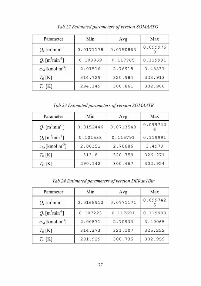
- 77 -
Tab.22 Estimated parameters of version SOMAATO
Parameter Min Avg Max
Qc [m3min-1] 0.0171178 0.0750863 0.0999769
Qr [m3min-1] 0.103969 0.117765 0.119991
cAi [kmol m-3] 2.01516 2.76918 3.48831
Tri [K] 314.729 320.984 323.913
Tci [K] 294.149 300.861 302.986
Tab.23 Estimated parameters of version SOMAATR
Parameter Min Avg Max
Qc [m3min-1] 0.0152446 0.0713548 0.0997426
Qr [m3min-1] 0.101533 0.115791 0.119991
cAi [kmol m-3] 2.00351 2.70686 3.4979
Tri [K] 313.8 320.759 326.271
Tci [K] 290.142 300.467 302.924
Tab.24 Estimated parameters of version DERan1Bin
Parameter Min Avg Max
Qc [m3min-1] 0.0165912 0.0771171 0.0997425
Qr [m3min-1] 0.107223 0.117691 0.119999
cAi [kmol m-3] 2.00871 2.70933 3.49065
Tri [K] 314.373 321.107 325.252
Tci [K] 291.929 300.735 302.959

- 78 -
Tab.25 Estimated parameters of version DERan2Bin
Parameter Min Avg Max
Qc [m3min-1] 0.0150441 0.076943 0.099324
Qr [m3min-1] 0.111014 0.117478 0.119987
cAi [kmol m-3] 2.00442 2.76267 3.4904
Tri [K] 314.342 320.982 323.118
Tci [K] 295.49 301.138 302.939
Tab.26 Estimated parameters of version GA
Parameter Min Avg Max
Qc [m3min-1] 0.0152769 0.0706135 0.0994583
Qr [m3min-1] 0.105348 0.115416 0.119818
cAi [kmol m-3] 2.00811 2.69678 3.49589
Tri [K] 314.177 320.645 324.491
Tci [K] 290.091 299.845 302.908
Tab.27 Estimated parameters of version SA_Elitism
Parameter Min Avg Max
Qc [m3min-1] 0.0153787 0.0720453 0.0998463
Qr [m3min-1] 0.108632 0.115819 0.119973
cAi [kmol m-3] 2.00362 2.82362 3.47147
Tri [K] 313.761 320.712 324.473
Tci [K] 292.07 300.187 302.983

- 79 -
Tab.28 Estimated parameters of version SA_NoElitism
Parameter Min Avg Max
Qc [m3min-1] 0.0162479 0.0733041 0.0998877
Qr [m3min-1] 0.103081 0.115918 0.119989
cAi [kmol m-3] 2.0153 2.7703 3.48319
Tri [K] 314.29 320.966 324.916
Tci [K] 292.525 300.063 302.977

- 80 -
a) Parameter variation (SOMAATO)
b) Parameter variation
(SOMAATO)-detail
c) Parameter variation (SOMAATR)
d) Parameter variation
(SOMAATR)-detail
e) Parameter variation (DERan1Bin)
f) Parameter variation (DERan1Bin)-detail
g) Parameter variation (DERan2Bin)
h) Parameter variation
(DERan2Bin)-detail
Fig. 29. Parameter variation of SOMA and DE for model CSTR

- 81 -
a) Parameter variation (SA_Elitism)
b) Parameter variation (SA_Elitism)-detail
c) Parameter variation (SA_NoElitism)
d) Parameter variation (SA_NoElitism)
e) Parameter variation (GA)
f). Parameter variation (GA)-detail
Fig. 30. Parameter variation of SA and GA for model CSTR
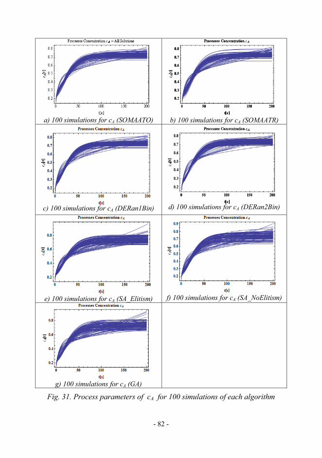
- 82 -
a) 100 simulations for cA (SOMAATO)
b) 100 simulations for cA (SOMAATR)
c) 100 simulations for cA (DERan1Bin) d) 100 simulations for cA (DERan2Bin)
e) 100 simulations for cA (SA_Elitism)
f) 100 simulations for cA (SA_NoElitism)
g) 100 simulations for cA (GA)
Fig. 31. Process parameters of cA for 100 simulations of each algorithm
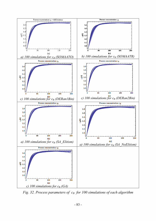
- 83 -
a) 100 simulations for cB (SOMAATO)
b) 100 simulations for cB (SOMAATR)
c) 100 simulations for cB (DERan1Bin) c) 100 simulations for cB (DERan2Bin)
a) 100 simulations for cB (SA_Elitism) a) 100 simulations for cB (SA_NoElitism)
c) 100 simulations for cB (GA)
Fig. 32. Process parameters of cB for 100 simulations of each algorithm

- 84 -
a) 100 simulations for Tr (SOMAATO)
b) 100 simulations for Tr (SOMAATR)
c) 100 simulations for Tr (DERan1Bin) c) 100 simulations for Tr (DERan2Bin)
a) 100 simulations for Tr (SA_Elitism)
a) 100 simulations for Tr (SA_NoElitism)
c) 100 simulations for Tr (GA)
Fig. 33. Process parameters of Tr for 100 simulations of each algorithm

- 85 -
a) 100 simulations for Tc (SOMAATO)
b) 100 simulations for Tc (SOMAATR)
c) 100 simulations for Tc (DERan1Bin)
c) 100 simulations for Tc (DERan2Bin)
a) 100 simulations for Tc (SA_Elitism)
a) 100 simulations for Tc (SA_NoElitism)
c) 100 simulations for Tc (GA)
Fig. 34. Process parameters of Tc for 100 simulations of each algorithm

- 86 -
5.3.5.4 Discussion and conclusion
Just as in the case mentioned in the previous section for optimization of batch reactor, all simulations were repeated 100 times for each EA with the same principle simulation evolutionary algorithms. The parameters setting for EAs is the same in the case of optimization for bacth reactor, only I have changed number migrations of parameters setting of SOMA from 50 to 10 in order to get speedier simulation. The optimization by the cost function with concentration cB show in (5.17) and time of each simulation is 200 seconds.
Calculation was 100 times repeated and the best, worst and average result (individual) was recorded from the last population in each simulation. All one hundred triplets (best, worst, average) were used to create Fig.29 & 30.
Compared with model of Batch, that the results from optimization on CSTR have obtained nearly resemblance. Estimated parameters and their diversity (minimum, maximum and average) are near approximately (see in Tab. 22-28). From the graphs of processes parameters for 100 simulations for cA, cB, Tr Tc (see Fig. 31-34) of each algorithm, it is very difficult to determine which algorithm is better. There are only small differences between them. On optimization of SOMA and DE, it is evident that the courses of algorithm are densities in a thin spectrum more than GA and SA. Alongside it, sometime few values drift out of the actual solution. But by the repetition of simulation was recorded the best result. On Fig. 35, the process of parameters by SOMA algorithm obtained best solution for the optimization.
Specially, there is difference between from both chosen model of chemical reactors (batch and CSTR). From investigation on optimization of process parameter of CSTR we can see, that four evolutionary algorithms (SOMA, DE, SA, GA) have obtained optimized results on very approximate value.
From these results we may conclude, that the quality and course of the evolutionary processes can be influenced by many factors, notably: setting parameters, definition of cost function, number of generations…. Moreover the results produced by the optimization process depends on the problem being solved, e.g. dynamical systems (mathematical and physical model).

- 87 -
a) Best solution for cA
a) Best solution for cB
c) Best solution for Tr
c) a) Best solution for Tc
Fig. 35. Best solution of SOMA

- 88 -
6 PREDICTIVE CONTROL
During the last decade, control scientists and experts have been thinking and given ideas in order to explore future directions of control theory and its applications. In addition, recent advances in computer technology, modern control techniques, and computational intelligence have opened a path for application of new generations of advanced process control algorithms (Takatsu et al., 1998; VanDoren, 1998).
Predictive control by mean evolutionary algorithms is very robust method, particular in system with many disturbing effects and failures. It's also a powerful tool in the search for optimal solutions to very complex problem in the field of control process. The basic idea is to find a set of action that lead to the principle optimization with required value. The block prediction procedure is shown in Fig. 36.
k+1k -1k
y(t) $ ( )y t
w
h isto ry fu ture
u(t)
tim eN1
k+Nu
Nu N2
k+ N2
Fig. 36. Principle of predictive control by evolutionary algorithm
Model of system
Algorithms optimization
System
w u y

- 89 -
In block „Algorithms optimization“ are evolutionary algorithms, the predictive control is selected by minimising the commonly cost function J:
∑∑==
−+Δ++−+=uN
j
N
Nju jkujjkwjkyNNNJ
1
2221 )]1()[()]()([),,(
2
1
λ (6.1)
Here y is the output of system, u is actuating signal, w is the controlled value prediction, Δu is the control value change, k is the control step, N1
is the lower and N2 is the upper output prediction horizon, Nu is control horizon and λ is a weight sequence control of action.
Block "system" is a control process and block "model system" is used to predict its behaviour, it often represented in the appropriate algorithms of artificial intelligent, commonly artificial neural network.
Predictive control proceed that when change of required value running optimization algorithms in conjunction with model of system and minimising cost function (6.1) is found optimal action, which is for chosen system.
6.1 Principle simulation
In simulation of predictive control were used non-linear models, which were described in “problem design” of batch reactor and “mathematical problems” of CSTR. It was used such as block “system” and “model of system”. The principle simulation shown in Fig. 37.

- 90 -
Fig. 37. Principle simulation
6.2 Optimization of CSTR value with prediction control
In this part of thesis, the temperature of CSTR reactor were chosen for prediction control. On this optimization the point was to minimize the area arising as a difference between the required and real temperature profile of the reaction mixture in a selected time interval, which was the duration of CSTR cycle. The cost functions that were minimized is given in (6.2) for Tc temperature and (6.3) for Tr.
[ ]∑
=
−=t
trt tTwf
01cos
(6.2)
[ ]∑
=
−=t
tct tTwf
02cos
(6.3)
Where w1 , w2 are required values (control points)
Mathematica Definition of parameters and starting EA.
Processing with form of graphics and tables
Return back best values and history running EA
Setting
parameters and starting EA
EA from AGO library (Coding of EA in
language Mathematica) Stop EA Start EA
Return back values of
functional for existing
individual to EA Valuation functional
with model of reactor
Cycle till stopping
Run EA and call functional in environment Mathematica
Functional for static optimization in environment
Mathematica

- 91 -
For static optimization of CSTR value with prediction control we have added required value for simulation of temperature Tr and Tc belong following below Tab.29 & 30. The range inside of temperature Tr and Tc for predictive is <273.;380> [K ].
Tab. 29 Range inside for predictive control of CSTR
Parameter Range
rT [K] 273 – 380
cT [K] 273 – 380
Tab. 30. Parameters setting for predictive control of CSTR Time
simulation[s] Required value w1
for rT [K] Required value w2
for cT [K]
0 - 80 360 340
80 - 150 340 320
150 - 200 320 300
200 - 300 370 370
Simulations were conducted so that the first minimising cost function using the prediction horizon is found within the optimal action and intervention that was held for the control horizon. After that was calculated new intervention and has been applied during control horizon etc. till to do filling of reactor. For the CSTR reactor was selected: N1 = 1, N2 =300 a Nu = till to change.
6.3 Results of predictive control
On investigation of predictive control chemical reactor CSTR, I have chosen one basic version of each algorithm to optimize process parameters reactor. Concretely: version SOMAATO for SOMA; version DERan1Bin for

- 92 -
DE; version SA Elitism for SA. The evolutionary algorithms have been applied 100 times and the evolutionary processes of four algorithms show in follow graphs from Fig. 38 - 41.
Fig. 38. Predictive control temperatures Tr and Tc of CSTR by SOMAATO, “red” was required value

- 93 -
Fig. 39. Predictive control temperatures Tr and Tc of CSTR by DERan1Bin, “red” was required value

- 94 -
Fig. 40. Predictive control temperatures Tr and Tc of CSTR by GA, “red” was required value

- 95 -
d) Evolutionary process for Tc
Fig. 41. Predictive control temperatures Tr and Tc of CSTR by SA_Elitism, “red” was required value

- 96 -
6.4 Discussion and conclusion to the results of predictive control
The work here is performed through predictive control on non-linear system using evolutionary algorithms SOMA, DE, SA GA. Based on the achieved results it can be stated as follows:
• EA is used successfully on predictive control of the chemical reactors' processes;
• In the previous section about part optimization process of chemical reactions, it cannot be fully confirmed if any one of the chosen algorithm produced better results than the others. However, from the image results shown above, it may be concluded that SOMA and DE algorithms are best for the predictive control (at least in this case). Specifically, it can be seen in figures 38-41 items (c) & (d) for evolutionary process Tr and Tc. All 100 simulations of SOMA and DE have obtained very approximate values, which evidently prove that the courses of algorithm are densities in a thin spectrum and they meet the required value more closely than GA and SA; and
• From the results obtained, it is found that the process of concentration cA was in inverse ratio to the process temperatures. When temperature of the reactant mixture and coolant increased, temperature of concentration cA decreased. And when the temperature was stable, the concentration too was stable. Only on the process of concentration cB did it appear to be failure. From interval time simulation 150-200, process of cB decreased in direct ratio to the temperatures, and from time simulation 200, failure appeared.
Finally, it can be asserted that EAs are certainly and completely capable of controlling simple faulted system. Nevertheless, this topic deserves further and more detailed study that goes beyond the scope of the work presented here.

- 97 -
7 RESULTS OF DISSERTASION THESIS AND
FURTHER RESEARCH PERSPECTIVE
7.1 Evaluation of the objectives
This thesis has identified six targets and the achievement of those targets are discussed here. The evaluation of each objective is contained in the information provided at the end of each chapter where the respective evaluation is carried out. Specifically:
The introduction of chemical engineering process, application domain of chemical reactions and reactors and analysis of chosen dynamic systems
The objective has been achieved. In the chapter "Chemical Engineering process" -- it is raised that this is the important period to analyse industrial producing system, especially of chemical engineering process in the industries. This chapter confirms that the application domain of chemical reactions and reactors constitute one of the backbones for interdisciplinary collaboration. In fact, the optimization of industrial chemical processes has drawn attention in recent years, and designing the optimal parameters of reactor and its control system is one of the most difficult tasks of process engineering. Here, the thesis uses as model case, two chemical reactors, namely Batch and CSTR (known as an expert proposed), for optimization. Finding the optimum parameters of the chemical reactor and the exact procedure will greatly aid in drawing up proposal for technological equipment that can meet the economic and quality demands placed on an industrial operation.
Analysis of evolutionary algorithm, principle simulation and selecting new methods of algorithms, from artificial intelligence to optimization and predictive control chemical reactor.
The objective has been achieved. Chapter 4 analysed and described very concretely about EAs and their principle in use. A brief survey of Scoping and Screening chemical reaction networks using stochastic optimization is

- 98 -
also raised in this chapter. Four algorithms from the field of artificial intelligence -- Differential evolution (DE), Self-organizing migrating algorithm (SOMA), Genetic algorithm (GA) and Simulated annealing (SA) -- are used in the investigation. In the first section, EAs are used investigate and optimize the batch reactor to improve its parameters. Consequently, EAs are used to model the technical requirements for chemical reaction. The second section presents the optimizing of chemical engineering processes, particularly those in which the evolutionary algorithm is used for static optimization and control of Continuously-stirred tank reactors (CSTRs).
Demonstrating successfully on simulation by mean evolutionary algorithms, the problem design model of chemical reactors and the practical method to optimize chemical processes.
The objective has been achieved. In chapter 5 "Simulation part" the optimization tool has been described and four EAs were selected, especially for a certified high robustness and the ability to successfully solve complex optimization problems. Mathematical model of the process, established on the basis of balance equations, coupled with other important relationships derived for the real reactor, are used to conduct simulations of experts to set the reactor for optimization. The aim of this work was to use artificial intelligence methods, namely evolutionary algorithms, for static optimization of chemical reactor in order to improve the quality of its behaviour.
Demonstrating the use of designed algorithms global optimization on the predictive control chemical processes and comparing between each selected algorithms.
The objective has been achieved. Here it is demonstrated that methods of artificial intelligence, mainly EA, are successfully applied to predictive control of a chemical reactor. The optimized reactor is used in a simulation with prediction control by evolutionary algorithms and the results are presented in graphs (see chapter 6).

- 99 -
7.2 General conclusion and further research perspective
In this thesis, evolutionary algorithms are used for static optimization of chemical reactors in order to improve the quality of their behaviour in the uncontrolled state and in predictive control. The optimization tool has been described and four EAs (SOMA, DE, SA and GA) are chosen, especially for a certified high robustness and the ability to successfully solve complex optimization problems of chemical reactors.
The optimization and control of the chemical reactors have been performed in several ways, each one for a different set of reactor parameters or different cost function. From the results obtained, it is possible to say that all simulations give satisfactory results and thus EAs are capable of solving this class of difficult problems. The quality of the results depends not only on the problems being solved, they are also extremely sensitive to the proper definition of the cost function and the selection of parameters setting of evolutionary algorithms.
In fact, methods of artificial intelligence, mainly evolutionary computational techniques, should be used in the difficult tasks of analysing and optimizing dynamical systems, especially of chemical reactors. The main aim of the dissertation is focused on examples of EA implementation on the methods for chemical reaction that could be robust and effective to optimize difficult problems in the field of chemical engineering, with the intent to obtain better results, i.e. efficiency in reaching the desired stable state and superior stabilization.
The basic optimization process presented here is based on a relatively simple function. Nevertheless, there is no problem in defining more complex functional including as subcriteria, e.g. stability, costs, time-optimal criteria, controllability and etc., or their arbitrary combinations; unless the experiment is limited by technical issues while searching for optimal parameters.
Future research of evolutionary algorithms SOMA, DE, GA and SA is still ongoing. Based to all results obtained from this current research, it is suggested that the main activities should be focused on the expanding of this study for other chemical dynamic systems.

- 100 -
It can be concluded from the results of this dissertation that EAs have shown great potential and ability to solve complex problems of optimization, not only in the fields of chemical engineering process but also in diverse industrial fields.

- 101 -
8 REFERENCES
[1] Achenie, L. E. K., and L. T. Biegler, ‘‘Algorithmic Synthesis of Chemical Reactor Networks Using Mathematical Programming,’’ Ind. Eng. Chem. Fundam., 25, 621 (1986).
[2] Achenie, L. E. K., and L. T. Biegler, ‘‘Developing Targets for the Performance Index of a Reactor Network,’’ Ind. Eng. Chem. Res., 27, 1811 (1988).
[3] Achenie, L. E. K., and L. T. Biegler, ‘‘A Superstructure Based Approach to Chemical Reactor Network Synthesis,’’ Comput. Chem.Eng., 14, 23 (1990).
[4] A.e. Eiben and j.e. Smith, Introduction to Evolutionary Computing, Springer, Natural Computing series1st edition, 2003, ISBN: 3-540-40184-9corr. 2nd printing, 2007, ISBN: 978-3-540-40184-1.
[5] Angira, Rakesh and B.V.Babu, "Optimization of Non-Linear Chemical Processes Using Modified Differential Evolution (MDE)", Proceedings of The 2nd Indian International Conference on Artificial Intelligence (IICAI-2005), Pune, India, December 20-22, 2005, pp. 911-923, 2005.
[6] Aris, R., ‘‘Studies in Optimisation. III. The Optimum Operating Conditions in Sequences of Stirred Tank Reactors,’’ Chem. Eng.Sci., 13, 75 (1960).
[7] Aris, R., ‘‘Studies in Optimisation_IV. The Optimum Conditions for a Single Reaction,’’ Chem. Eng. Sci., 13, 197 (1961).
[8] Aziz N., Hussain M.A., Mujtaba I.M. (2000). Performance of different types of controllers in tracking optimal temperature in batch reactors. Computers and Chemical Engineering, Vol. 27, p. 1069-1075.
[9] B. Naderi, M. Zandieh, A. Khaleghi Ghoshe Balagh, V. Roshanaei, An improved simulated annealing for hybrid flowshops with sequence-dependent setup and transportation times to minimize total completion time and total tardiness, Expert Systems with Applications, Volume 36, Issue 6, August 2009, Pages 9625-9633, ISSN 0957-4174, DOI: 10.1016/j.eswa.2008.09.063.

- 102 -
[10] Balakrishna, S., and L. T. Biegler, ‘‘Constructive Targeting Approaches to the Synthesis of Chemical Reactor Networks,’’ Ind. Eng. Chem. Res., 31, 300 (1992a.).
[11] Balakrishna, S., and L. T. Biegler, ‘‘Targeting Strategies for the Synthesis and Energy Integration of Nonisothermal Reactor Networks,’’ Ind. Eng. Chem. Res., 31, 2152 (1992b).
[12] Beasley, D. 1997 Possible applications of evolutionary computation. In B¨ack, T., Fogel, D. B. &Michalewicz, Z., editors, Handbook of Evolutionary Computation. 97/1, A1.2, IOP Publishing Ltd. and Oxford University Press.
[13] Béla G. Lipták, Instrument Engineers' Handbook: Process control and optimization. Edition: 4, illustrated. Published by CRC Press, 2003. ISBN 0849310814, 9780849310812. 2464 pages.
[14] Bruce Nauman, E. Chemical Reactor Design, Optimization, and Scale up, IBSN 0-07-137753-0.
[15] Chitra, S. P., and R. Govind, ‘‘Yield Optimization for Complex Reaction Systems,’’ Chem. Eng. Sci., 36, 1219 (1981).
[16] Chitra, S. P., and R. Govind, ‘‘Synthesis of Optimal Serial Reactor Structures for Homogeneous Reactions. Part I: Isothermal Reactors,’’ AIChE J., 31, 177 (1985a.).
[17] Chitra, S. P., and R. Govind, ‘‘Synthesis of Optimal Serial Reactor Structures for Homogeneous Reactions. Part II: Nonisothermal Reactors,’’ AIChE J., 31, 185 (1985b).
[18] Corriou, J.P. (2004). Process control. Theory and applications. Springer-Verlag, London.
[19] Dasgupta, D. and Michalewicz, Z., .Evolutionary algorithms in Engineering Applications., Springer, Germany, pp 3-23 (1997).
[20] Dostál, P., V. Bobál and M. Blaha (2001). One approach to adaptive control of nonlinear processes. In: Proc. IFAC Workshop on Adaptation and Learning in Control and Signal Processing ALCOSP 2001, Cernobbio-Como, Italy, 407-412.

- 103 -
[21] Dostál, P., Gazdoš, F., Bobál, V., Vojtěšek, J.: Adaptive control of a continuous stirred tank reactor By two feedback controllers. In: 9th IFAC Workshop Adaption and Learning in Kontrol and Sinal Processing ALCOSP’2007, Saint Petersburg, Russia, August 29-31, 2007, P5-1 – P5-6.
[22] Dyson, D. C., and J. M. Horn, ‘‘Optimum Distributed Feed Reactors for Exothermic Reversible Reactions,’’ J. Optimiz. Theory Appl., 1, 40 (1967).
[23] Dyson, D. C., and J. M. Horn, ‘‘Optimum Adiabatic Cascade Reactor with Direct Intercooling,’’ Ind. Eng. Chem. Fundam., 8, 49 (1969).
[24] Emuoyibofarhe O.Justice., Reju A Sunday, An optimum solution for a process control problem (continuous stirred tank reactor) using a hybrid neural network. Journal of Theoretical and Applied Information Technology. Volume 4, Number 10, Pages: 906-915. 31 October 2008.
[25] Floudas, C. A., .Nonlinear and Mixed-Integer Optimization., New York, Oxford University Press (1995).
[26] Glover F., Laguna M. a Martí R., Scatter Search in Ghosh A. a Tsutsui S. (Eds.), Advances in Evolutionary Computation: Theory and Applications, Springer-Verlag, New York, pp. 519-537, 2003.
[27] Gross B.; Roosen P. Total process optimization in chemical engineering with evolutionary algorithms. Computers & Chemical Engineering. Volume 22, Supplement 1, 15 March 1998, Pages S229-S236. European Symposium on Computer Aided Process Engineering-8.
[28] Glasser, D., D. Hildebrandt, and C. M. Crowe, ‘‘A Geometric Approach to Steady Flow Reactors: The Attainable Region and Optimization in the Concentration Space,’’ Ind. Eng. Chem. Res., 26, 1803 (1987).
[29] Glasser, D., D. Hildebrandt, and S. Godorr, ‘‘The Attainable Region for Segregated Maximum Mixed and Other Reactor Models,’’ Ind. Eng. Chem. Res., 33, 1136 (1994).

- 104 -
[30] Glasser, B., D. Hildebrandt, and D. Glasser, ‘‘Optimal Mixing for Exothermic Reversible Reactions,’’ Ind. Eng. Chem. Res., 31, 1541 (1992).
[31] Glasser, D., and D. Hildebrandt, ‘‘Reactor and Process Synthesis,’’ Comput. Chem. Eng., 21, S775 (1997).
[32] Godorr, S., D. Hildebrandt, D. Glasser, and C. McGregor, ‘‘Choosing Optimal Control Policies Using the Attainable Region Approach,’’ Ind. Eng. Chem. Res., 38, 639 (1999).
[33] Hildebrandt, D., and L. T. Biegler, ‘‘Synthesis of Chemical Reactor Networks,’’ FOCAPD, Snowmass, CO (1994).
[34] Hildebrandt, D., and D. Glasser, ‘‘The Attainable Region and Optimal Reactor Structures,’’ Chem. Eng. Sci., 45, 2161 (1990).
[35] Hildebrandt, D., D. Glasser, and C. M. Crowe, ‘‘Geometry of the Attainable Region Generated by Reaction and Mixing: With and Without Constraints,’’ Ind. Eng. Chem. Res., 29, 49 (1990).
[36] Hopley, F., D. Hildebrandt, and D. Glasser, ‘‘Optimal Reactor Structures for Exothermic Reversible-Reactions with Complex kinetics,’’ Chem. Eng. Sci., 51, 2399 (1996).
[37] Horn, F., ‘‘Attainable and Non-Attainable Regions in Chemical Reaction Technique,’’ Proc. Euro. Symp. on Chemical Reaction Engineering, Pergamon Press, London (1964).
[38] Hildebrandt, D., and L. T. Biegler, ‘‘Synthesis of Chemical Reactor Networks,’’ FOCAPD, Snowmass, CO (1994).
[39] Ingham, J., Dunn, I.J., Heinzle, E., J.E.P 2000. Chemical Engineering Dynamic, ISBN 3-527-29776-6.
[40] Ivo F. Sbalzarini, Sibylle Muller and Petros Koumoutsakos 2000. Multiobjective optimization using evolutionary algorithms. Center for Turbulence Research, Proceedings of the Summer Program 2000.
[41] Jackson, R., ‘‘Optimization of Chemical Reactors with Respect to Flow Configuration,’’ J. Optimiz. Theory Appl., 2, 240 (1968).

- 105 -
[42] Kirkpatrick S., Gelatt Jr., C.D., Vecchi, M.P., Optimization by Simulated Annealing, Science, vol. 220, no. 4598, 671-680, (1983).
[43] Kokossis, A. C., and C. A. Floudas, ‘‘Optimization of Complex Reactor Networks: I. Isothermal Operation,’’ Chem. Eng. Sci., 45, 595 (1990).
[44] Kokossis, A. C., and C. A. Floudas, ‘‘Synthesis and Optimization of Isothermal Reactor Separator Recycle Systems,’’ Chem. Eng. Sci., 46, 261 (1991).
[45] Kokossis, A. C., and C. A. Floudas, ‘‘Optimization of Complex Reactor Networks: II. Nonisothermal Operation,’’ Chem. Eng. Sci., 49, 1037 (1994).
[46] Lakshmanan, A., and L. T. Biegler, ‘‘Reactor Network Targeting for Waste Minimization,’’ Pollution Prevention via Process and Product Modifications, AIChE Symp. Ser. 90, M. El-Halwagi and D. Petrides, eds., AIChE, New York, p. 128 (1994).
[47] Lakshmanan, A., and L. T. Biegler, ‘‘Synthesis of Optimal Chemical Reactor Networks,’’ Ind. Eng. Chem. Res., 35, 1344 (1996).
[48] Lakshmanan, A., and L. T. Biegler, ‘‘A Case Study for Reactor Network Synthesis: The Vinyl Chloride Process,’’ Comput. Chem. Eng.,21, S785 (1997).
[49] Levenspiel O. Chemical reaction engineering. New York: John Wiley and Sons, 1962. 578 p.
[50] Li, Y. and Haubler, A. Artificial evolution of neural networks and its application to feedback control. Artificial Intelligence in Engineering 10, 143-152 (1996).
[51] Liu et al., 2007 Li Liu, Wenxin Liu and David A. Cartes, Particle swarm optimization-based parameter identification applied to permanent magnet synchronous motors, Engineering Applications of Artificial Intelligence (2007) 10.1016/j.engappai.2007.10.002.

- 106 -
[52] Marcoulaki, E. C., Kokossis, A. C., Scoping and screening complex reaction networks using stochastic optimization , AIChE Journal, Volume 45 Issue 9, Pages 1977 – 1991.
[53] Mansour, M. J.E. Ellis, Methodology of on-line optimisation applied to a chemical reactor Applied Mathematical Modelling, Volume 32, Issue 2, February 2008, Pages 170-184.
[54] McGregor, C., D. Glasser, and D. Hildebrandt, ‘‘The Attainable Region and Pontryagin’s Maximum Principle,’’ Ind. Eng. Chem. Res., 38, 652 (1999).
[55] Mylene C.A.F. Rezende, Caliane B.B. Costa, Aline C. Costa, M.R.Wolf Maciel, Rubens Maciel Filho. Optimization of a large scale industrial reactor by genetic algorithms. (2007).
[56] N. Metropolis, A.W. Rosenbluth, M.N. Rosenbluth, A.H. Teller and E. Teller, Equation of state calculations by fast computing machines, Journal of Chemical Physics 21 (6) (1953), pp. 1087–1092.
[57] Ng, D. Y. C., and D. W. T. Rippin, ‘‘The Effect of Incomplete Mixing on Conversion in Homogeneous Reactions,’’ Proc. Euro. Symp. on Chemical Reaction Engineering, Pergamon Press, Oxford (1965).
[58] Nolle et al., 2001 L. Nolle, A. Goodyear, A.A. Hopgood, P.D. Picton and Braithwaite, N.StJ.: on step width adaptation in simulated annealing for continuous parameter optimisation. In: B. Reusch, Editor, Computational Intelligence—Theory and Applications, Lecture Notes in Computer Science vol. 2206, Springer, Berlin (2001), pp. 589–598. Full Text via CrossRef
[59] Nolle et al., 2005 L. Nolle, I. Zelinka, A.A. Hopgood and A. Goodyear, Comparison of an self organizing migration algorithm with simulated annealing and differential evolution for automated waveform tuning, Advances in Engineering Software 36 (10) (2005), pp. 645–653.
[60] Nisoli, A., M. F. Malone, and M. F. Doherty, ‘‘Attainable Regions for Reaction with Separation,’’ AIChE J., 43, 374 (1997)
[61] Ogunnaike, B.A. and W.H. Ray (1994). Process dynamics, modelling, and control. Oxford University Press, New York.

- 107 -
[62] Paynter, J. D., and D. E. Haskins, ‘‘Determination of Optimal Reactor Type,’’ Chem. Eng. Sci., 25, 1415 (1970).
[63] Pham, Q.T. Dynamic optimization of chemical engineering processes by evolutionary method (2005).
[64] Pham, Q.T. and Coulter, S., Modelling the chilling of pig carcasses using an evolutionary method. Proc. Int. Congress of Refrig. Vol. 3a pp.676-683 (1995).
[65] Po-Han Chen, Seyed Mohsen Shahandashti, Hybrid of genetic algorithm and simulated annealing for multiple project scheduling with multiple resource constraints, Automation in Construction, Volume 18, Issue 4, July 2009, Pages 434-443, ISSN 0926-5805, DOI: 10.1016/j.autcon.2008.10.007.
[66] Price, 1999 K. Price, An introduction to differential evolution. In: D. Corne, M. Dorigo and F. Glover, Editors, New Ideas in Optimization, McGraw-Hill, London, UK (1999), pp. 79–108.
[67] Ravimohan, A. L., ‘‘Optimization of Chemical Reactor Networks with Respect to Flow Configuration,’’ J. Optimiz. Theory Appl., 8, 204 (1971).
[68] Rojnuckarin, A., C. A. Floudas, H. Rabitz, and R. A. Yetter, ‘‘Methane Conversion to Ethylene and Acetylene: Optimal Control with Chlorine, Oxygen, and Heat Flux,’’ Ind. Eng. Chem. Res., 35, 683 (1996).
[69] Salcedo, R. L., .Solving Nonconvex Nonlinear Programming Problems with Adaptive Random Search.. Industrial & Engineering Chemistry Research, 31, 262 (1992).
[70] Silva C.M., Biscaia E.C. (2003). Genetic algorithm development for multi-objective optimization of batch free-radical polymerization reactors. Computers and Chemical Engineering, Vol. 27, p. 1329-1344.
[71] S. Kirkpatrick, C.D. Gelatt Jr and M.P. Vecchi, Optimization by simulated annealing, Science 220 (4598) (1983), pp. 671–680.

- 108 -
[72] Schmidt, L.D. (2005). The engineering of chemical reactions. Oxford University Press, New York.
[73] Schweiger, C. A., and C. A. Floudas, ‘‘Optimization Framework for the Synthesis of Chemical Reactor Networks,’’ Ind. Eng. Chem. Res., 38, 744 (1999).
[74] Smith, R. Chemical Process, Design and Integration 2005, ISBN 0-471-48681-7.
[75] Srinisavan B., Palanki S., Bonvin D. (2002). Dynamic optimization of batch processes II. Role of Measurement in handling uncertainly. Computers and Chemical Engineering, Vol. 27, p. 27-44.
[76] Srinivasan et al., 2003 B. Srinivasan, S. Palanki and D. Bonvin, Dynamic optimization of batch processes: I. Characterization of the nominal solution, Computers & Chemical Engineering 27 (2003), pp. 1–26.
[77] Stericker, D.L. and N.K. Sinha (1993). Identification of continuous-time systems from samples of input-output data using the δ-operator. Control-Theory and Advanced Technology, 9, 113-125.
[78] Takatsu, H., Itoh, T., Araki, M. “Future needs for the control theory in industries report and topics of the control technology survey in Japanese industry”, Journal of Process Control, vol. 8, nos. 5-6, pp. 369-374, 1998.
[79] T. Backx, O. Bosgra, W. Marquardt, Integration of model predictive control and optimization of processes, in: Proceedings ADCHEM 2000, vol. 1, 2000, pp. 249–260.
[80] Wolpert, D.H., Macready, W.G. (1997), "No Free Lunch Theorems for Optimization," IEEE Transactions on Evolutionary Computation. Pages 68-72, Volume 1.
[81] Wong, J., .Computational Experience with a General Nonlinear Programming Algorithm.. COED J., 10, 19 (1990).

- 109 -
[82] Zelinka, I., 2004. SOMA—self organizing migrating algorithm. In: Babu, B.V., Onwubolu, G. (Eds.), New Optimization Techniques in Engineering. Springer, New York, pp. 167–218.
[83] Zelinka I. (2004) SOMA. In: B.V. Babu, G. Onwubolu Eds., New optimization techniques in engineering, Springer- Verlag, chapter 7, ISBN 3-540-20167-X
[84] Zelinka I. (2004) SOMA. In: B.V. Babu, G. Onwubolu Eds., New optimization techniques in engineering, Springer- Verlag, chapter 7, ISBN 3-540-20167-X
[85] Zelinka, I., Nolle, L., 2006. Plasma reactor optimizing using differential evolution. In: Price, K.V., Lampinen, J., Storn, R. (Eds.), Differential Evolution: A Practical Approach to Global Optimization. Springer, New York, pp. 499–512.
[86] Zelinka, I., 2004. SOMA—self organizing migrating algorithm. In: Babu, B.V., Onwubolu, G. (Eds.), New Optimization Techniques in Engineering. Springer, New York, pp. 167–218.
[87] Zelinka, I. Real-time deterministic chaos control by means of selected evolutionary techniques, Engineering Applications of Artificial Intelligence, Volume 22, Issue 2, March 2009, Pages 283-297, ISSN 0952-1976, DOI: 10.1016/j.engappai.2008.07.008.

- 110 -
LIST OF AUTHOR’S PUBLICATION ACTIVITIES
[1] Tran, T.D., Zelinka, I., Optimization of reactive distillation processes using Self-organizing Migrating Algorithm and Differential Evolution Strategies.(14th International Conference on Soft Computing MENDEL 2008, Brno, Czech Republic, Jun 18-20, 2008. P.186-191). ISBN: 978-80-214-3675-6.
[2] Tran, T.D., Zelinka, I., Investigation on Optimization of Chemical Process. (Seventh international conference on soft computing applied in computer and economic environments – ICSC 2009, Kunovice, Czech Republic, January 23, 2009). ISBN:978-80-7314-163-9.
[3] Tran, T.D., Zelinka, I., Dostál, P., Using evolutionary algorithm for simulation and optimization a continuous stirred tank reactor. – in Press, (submit to the Journal of Chemical Engineering).
[4] Tran, T.D., Zelinka, I., Investigation on Optimization of Process Parameters and Chemical Reactor Geometry by Evolutionary Algorithms. (23rd European Conference on Modelling and Simulation – ECMS 2009, Madrid, Spain June 9th - 12th, 2009).
[5] Tran, T.D., Zelinka, I.,Using method of artificial intelligence to optimise and control chemical reactor. (15th International Conference on Soft Computing MENDEL 2009, Brno, Czech Republic, Jun 24-26, 2009.
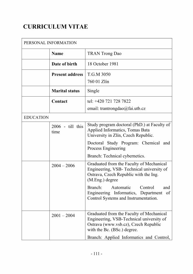
- 111 -
CURRICULUM VITAE
PERSONAL INFORMATION
Name TRAN Trong Dao
Date of birth 18 October 1981
Present address T.G.M 3050 760 01 Zlín
Marital status Single
Contact tel: +420 721 728 7822 email: [email protected]
EDUCATION
2006 - till this time
Study program doctoral (PhD.) at Faculty of Applied Informatics, Tomas Bata University in Zlín, Czech Republic.
Doctoral Study Program: Chemical and Process Engineering
Branch: Technical cybernetics.
2004 – 2006 Graduated from the Faculty of Mechanical Engineering, VSB- Technical university of Ostrava, Czech Republic with the Ing. (M.Eng.) degree
Branch: Automatic Control and Engineering Informatics, Department of Control Systems and Instrumentation.
2001 – 2004 Graduated from the Faculty of Mechanical Engineering, VSB-Technical university of Ostrava (www.vsb.cz), Czech Republic with the Bc. (BSc.) degree.
Branch: Applied Informatics and Control,

- 112 -
Department of Control Systems and Instrumentation.
2001 Moved to study in the Czech Republic.
5/2001 – 9/2001 Graduated course Czech language at The Department of Foreign Languages of VŠB-Technical University of Ostrava.
1999 – 2000 Student of Hanoi University of Mining and Geology. Study at the field of petroleum and gas complex.
1996 – 1999 Student of High school Tran Quoc Tuan, Quang Ngai, Vietnam. GCE in Vietnamese language, English language, Mathematics and natural science.
SCHOLARSHIPS AND ATTENDENCE AT CONFERENCES
October 2006– October 2009
Scholarship under the program doctoral study at the Tomas Bata University in Zlin. Extra scholarship from Faculty Applied Informatics for success in the study and science in the academic year 2007/2008.
2007-2009 Attendance at international conference: Mendel’08 and Mendel’09 in Brno, Czech Republic; ICSC 2009 in Kunnovice, Czech Republic; ECMS 2009 in Madrid, Spain.
LANGUAGE KNOWLEDGE
Vietnamese language
native
English language
active – doctoral exam – July 2007
Czech language fluent

- 113 -
OTHER ACTIVITIES
Award for the “Star of January” from Vietnamese Student Association in Hanoi, Vietnam 2005. Diploma from Ambassador of Vietnam in the Czech Republic. Diploma from Vietnamese Youth and Student association, Hanoi, Vietnam 2006 - 2007.

- 114 -