2/23/21

1

Topic 4: Genetic CircuitsA. Integrated model of gene expression

1. constitutive gene expression2. transcription control3. translation control and mRNA stability4. control of protein degradation

B. Simple circuits using only transcriptional control1. negative autoregulation2. positive autoregulation3. toggle switch4. oscillators

C. Noise in gene expressionD. Metabolic control

1. gene regulation2. effect of inducer3. metabolic feedback

1

C. Genetic noise• extrinsic: variation of “external factors”, e.g., RNAp, ribosome, temp, …• intrinsic: stochasticity in mRNA and protein synthesis, TF-DNA binding,…! cell-to-cell variability if noise is amplified by feedback! escape from one state to another within a single cell

Q: fraction of total noise from extrinsic/intrinsic sources?

( )22int 2

c y

c yη

−=

LOW extrinsic noise and HIGH intrinsic noise:

uncorrelated fluctuationsPut two fluorescent proteins under the control of identical promoters.

HIGH extrinsic noise and LOW intrinsic noise:

highly correlated variations

2ext

cy c yc y

η−

=

2

2/23/21

2

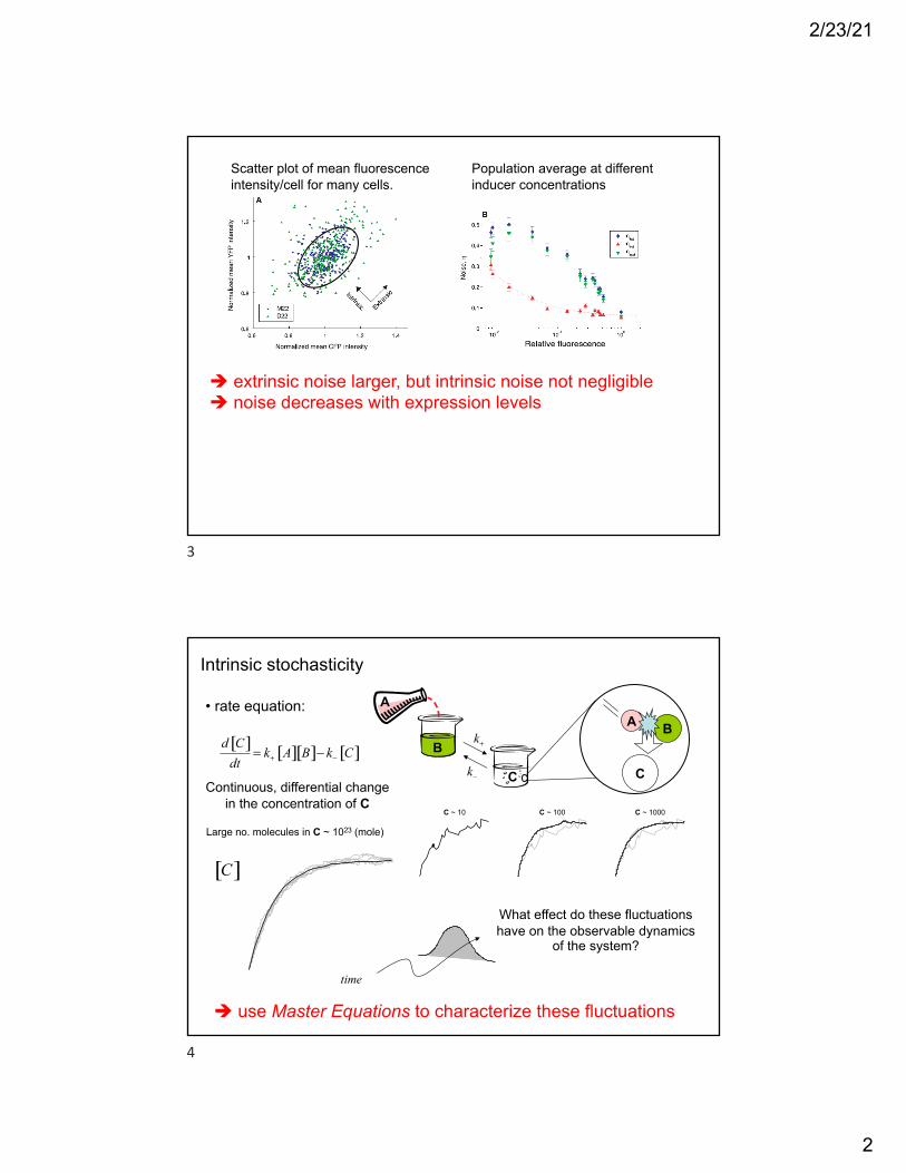
Scatter plot of mean fluorescence intensity/cell for many cells.

! extrinsic noise larger, but intrinsic noise not negligible! noise decreases with expression levels

Population average at different inducer concentrations

3

C

k+

k−

B

A

C

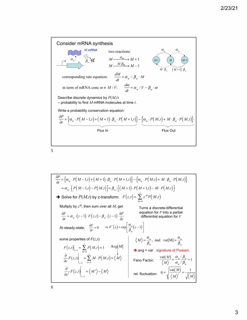
BA[ ] [ ][ ] [ ]d C

k A B k Cdt + −= −

Continuous, differential change in the concentration of C

C ~ 10 C ~ 100 C ~ 1000

[ ]C

time

What effect do these fluctuations have on the observable dynamics

of the system?

Large no. molecules in C ~ 1023 (mole)

! use Master Equations to characterize these fluctuations

Intrinsic stochasticity

• rate equation:

4

2/23/21

3

Consider mRNA synthesis

βmαm M-1 M+1M

αm αm

M +1( ) ⋅ βmM ⋅ βm

two reactions:

M αm ⎯ →⎯⎯ M +1

M M ⋅βm⎯ →⎯⎯⎯ M −1

Describe discrete dynamics by P(M,t)– probability to find M mRNA molecules at time t.

Write a probability conservation equation:∂P∂t

= αm ⋅ P M −1,t( ) + M +1( ) ⋅ βm ⋅ P M +1,t( ){ } − αm ⋅ P M ,t( ) + M ⋅ βm ⋅ P M ,t( ){ }Flux In Flux Out

M mRNA

corresponding rate equation: dMdt

= αm − βm ⋅ M

in term of mRNA conc m ≡ M /V: dmdt

= αm /V − βm ⋅m

5

Multiply by zM, then sum over all M, get

∂F∂t

= αm ⋅ z −1( ) ⋅ F z,t( ) − βm ⋅ z −1( ) ⋅ ∂F∂z

Turns a discrete-differential equation for P into a partial differential equation for F

At steady-state, 0Ft

∂ =∂

⇒ F * z( ) = exp αm

βmz −1( )⎡

⎣⎢

⎤

⎦⎥

∂P∂t

= αm ⋅ P M −1,t( ) + M +1( ) ⋅ βm ⋅ P M +1,t( ){ } − αm ⋅ P M ,t( ) + M ⋅ βm ⋅ P M ,t( ){ } = αm ⋅ P M −1,t( ) − P M ,t( )⎡⎣ ⎤⎦ + βm ⋅ M +1( ) ⋅ P M +1,t( ) − M ⋅ P M ,t( )⎡⎣ ⎤⎦

! Solve for P(M,t) by z-transform: F z,t( ) = z M P M ,t( )M =0

∞

∑

some properties of F(z,t):

F z,t( )z=1

= P M ,t( ) = 1M =0

∞

∑∂∂zF(z,t)

z=1

= M ⋅ P M ,t( )m=0

∞

∑ = M

∂2

∂z2F z,t( )

z=1

= M 2 − M

Avg[M]M =

αm

βm, and var[M] =

αm

βm! avg = var signature of Poisson

Fano Factor:var[M ]M

=αm / βmαm / βm

= 1

rel. fluctuation: η =var[M ]

M2 =

1

M

6

2/23/21

4

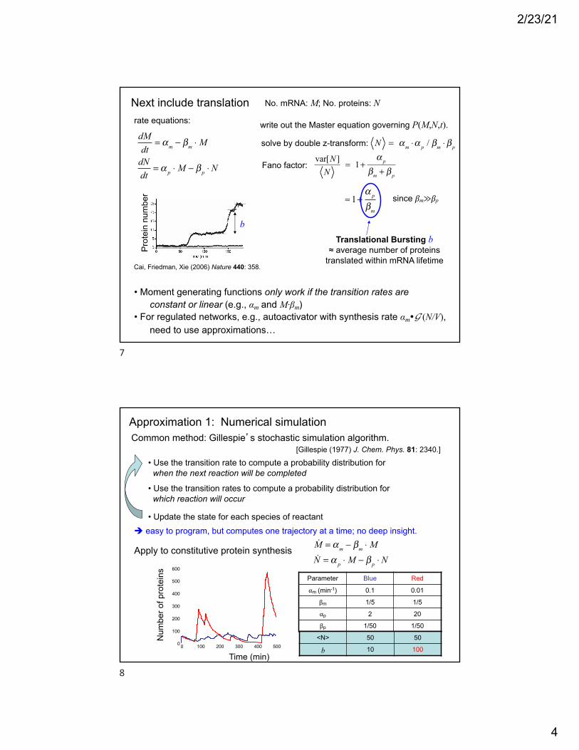
Next include translation

dMdt

= αm − βm ⋅ M

dNdt

= α p ⋅ M − β p ⋅ N

write out the Master equation governing P(M,N,t).

solve by double z-transform:

var[N ]N

= 1+α p

βm + β p

since βm≫βp≈ 1+α p

βm

Translational Bursting b≈ average number of proteins

translated within mRNA lifetime

• Moment generating functions only work if the transition rates areconstant or linear (e.g., αm and M·βm)

• For regulated networks, e.g., autoactivator with synthesis rate αm"G (N/V),need to use approximations…

b

Prot

ein

num

ber

Cai, Friedman, Xie (2006) Nature 440: 358.

rate equations:

N = αm ⋅α p / βm ⋅ β p

Fano factor:

No. mRNA: M; No. proteins: N

7

Approximation 1: Numerical simulation Common method: Gillespie’s stochastic simulation algorithm.

• Use the transition rate to compute a probability distribution for when the next reaction will be completed

• Use the transition rates to compute a probability distribution for which reaction will occur

• Update the state for each species of reactant! easy to program, but computes one trajectory at a time; no deep insight.

[Gillespie (1977) J. Chem. Phys. 81: 2340.]

Apply to constitutive protein synthesis

0 100 200 300 400 5000

100

200

300

400

500

600

Num

ber o

f pro

tein

s

Time (min)

Parameter Blue Red

αm (min-1) 0.1 0.01

βm 1/5 1/5

αp 2 20

βp 1/50 1/50

M = αm − βm ⋅ MN = α p ⋅ M − β p ⋅ N

<N> 50 50

b 10 100

8

2/23/21

5

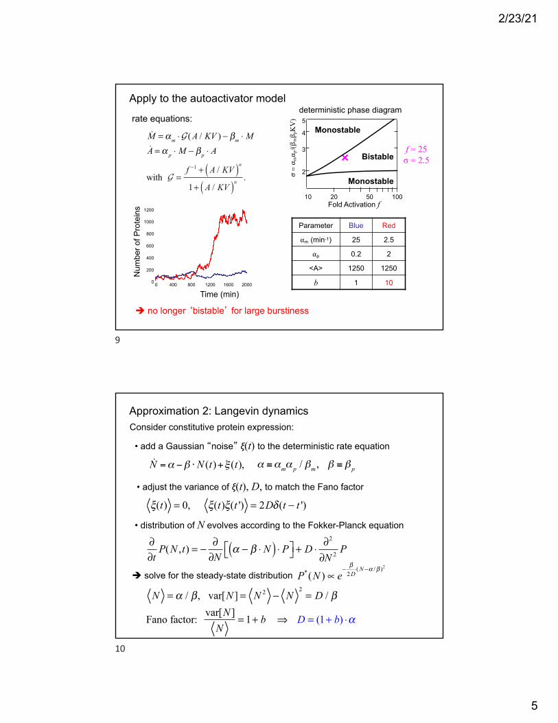
Apply to the autoactivator model

0 400 800 1200 1600 20000

200

400

600

800

1000

1200

Time (min)

Num

ber o

f Pro

tein

s

Parameter Blue Red

αm (min-1) 25 2.5

αp 0.2 2

<A> 1250 1250

b 1 10

f = 25σ = 2.5

M = αm ⋅G (A / KV ) − βm ⋅ MA = α p ⋅ M − β p ⋅ A

with G =f −1 + A / KV( )n1+ A / KV( )n

.

rate equations:

Fold Activation f

2Monostable

Bistable3

4

5

10 10020 50

Monostable

σ= α mα p

/(βmβ pKV)

deterministic phase diagram

! no longer ‘bistable’ for large burstiness

9

Approximation 2: Langevin dynamics

• add a Gaussian “noise” ξ(t) to the deterministic rate equation

!N =α −β ⋅N (t)+ξ (t), α ≡αmα p / βm , β ≡ β p

• adjust the variance of ξ(t), D, to match the Fano factor

ξ(t) = 0, ξ(t)ξ(t ') = 2Dδ (t − t ')

Consider constitutive protein expression:

• distribution of N evolves according to the Fokker-Planck equation

∂∂tP(N ,t) = −

∂∂N

α − β ⋅ N( ) ⋅ P⎡⎣ ⎤⎦ + D ⋅∂2

∂N 2 P

! solve for the steady-state distribution P*(N ) ∝ e−

β2D(N −α /β )2

N = α / β, var[N ] = N 2 − N2= D / β

Fano factor: var[N ]N

= 1+ b ⇒ D = (1+ b) ⋅α

10

2/23/21

6

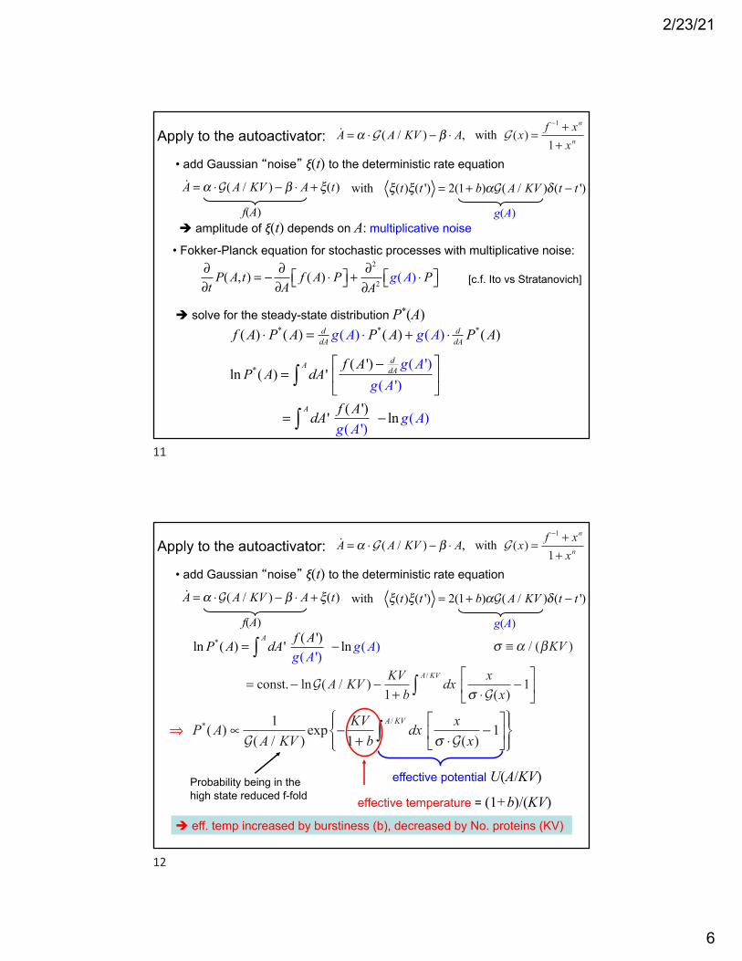
• add Gaussian “noise” ξ(t) to the deterministic rate equation A = α ⋅G(A / KV ) − β ⋅ A+ ξ(t)

! amplitude of ξ(t) depends on A: multiplicative noise

with ξ(t)ξ(t ') = 2(1+ b)αG(A / KV )δ (t − t ')

Apply to the autoactivator:

• Fokker-Planck equation for stochastic processes with multiplicative noise: ∂∂tP(A,t) = −

∂∂A

f (A) ⋅ P⎡⎣ ⎤⎦ +∂2

∂A2g(A) ⋅ P⎡⎣ ⎤⎦

! solve for the steady-state distribution P*(A)

A = α ⋅G (A / KV ) − β ⋅ A, with G (x) =f −1 + xn

1+ xn

f(A) g(A)

[c.f. Ito vs Stratanovich]

f (A) ⋅ P*(A) = ddA g(A) ⋅ P

*(A) + g(A) ⋅ ddA P*(A)

ln P*(A) = dA ' f (A ') − d

dA g(A ')g(A ')

⎡

⎣⎢

⎤

⎦⎥

A

∫

= dA ' f (A ')g(A ')

A

∫ − ln g(A)

11

• add Gaussian “noise” ξ(t) to the deterministic rate equation A = α ⋅G(A / KV ) − β ⋅ A+ ξ(t) with ξ(t)ξ(t ') = 2(1+ b)αG(A / KV )δ (t − t ')

Apply to the autoactivator: A = α ⋅G (A / KV ) − β ⋅ A, with G (x) =f −1 + xn

1+ xn

f(A) g(A)

ln P*(A) = dA ' f (A ')g(A ')

A

∫ − ln g(A)

Probability being in the high state reduced f-fold

= const.− lnG(A / KV ) −KV

1+ bdx

xσ ⋅G(x)

−1⎡

⎣⎢

⎤

⎦⎥

A/KV

∫

⇒ P*(A) ∝1

G(A / KV )exp −

KV1+ b

dx x

σ ⋅G(x)−1

⎡

⎣⎢

⎤

⎦⎥

A/KV

∫⎧⎨⎪

⎩⎪

⎫⎬⎪

⎭⎪

effective potential U(A/KV)

effective temperature = (1+b)/(KV)! eff. temp increased by burstiness (b), decreased by No. proteins (KV)

σ ≡ α / (βKV )

12

2/23/21

7

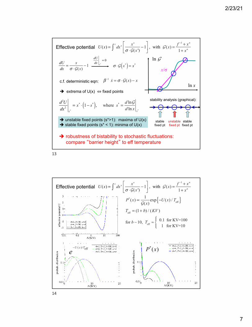
Effective potential U (x) = dx ' x '

σ ⋅G(x ')−1

⎡

⎣⎢

⎤

⎦⎥

x

∫ , with G (x) =f −1 + xn

1+ xn

dUdx

=x

σ ⋅G(x)−1

dUdx

x*= 0

σ ⋅G x*( ) = x*

c.f. deterministic eqn: β−1 x = σ ⋅G(x) − x

! extrema of U(x) ⇔ fixed points

d 2Udx2

x*

= x* ⋅ 1− s*( ), where s* =d lnGd ln x

x*

! unstable fixed points (s*>1): maxima of U(x)! stable fixed points (s* < 1): minima of U(x)

unstablefixed pt

stablefixed pt

stablefixed pt

stability analysis (graphical):

ln G

ln x

x/σ

! robustness of bistability to stochastic fluctuations: compare “barrier height” to eff temperature

13

Effective potential U (x) = dx ' x '

σ ⋅G(x ')−1

⎡

⎣⎢

⎤

⎦⎥

x

∫ , with G (x) =f −1 + xn

1+ xn

P*(x) ∝1G(x)

exp −U (x) / Teff{ }

Teff = (1+ b) / (KV )

for b ~ 10, Teff ≈0.1 for KV=1001 for KV=10

⎧⎨⎪

⎩⎪

e−U ( x )/Teff P*(x)

14

2/23/21

8

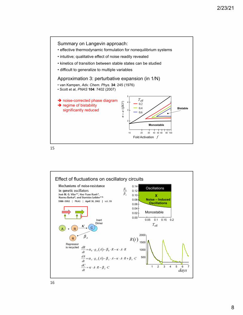
Summary on Langevin approach: • effective thermodynamic formulation for nonequilibrium systems• intuitive; qualitative effect of noise readily revealed• kinetics of transition between stable states can be studied• difficult to generalize to multiple variables

Approximation 3: perturbative expansion (in 1/N)• van Kampen, Adv. Chem. Phys. 34: 245 (1976)• Scott et al, PNAS 104: 7402 (2007)

Fold Activation

2

Monostable

Bistable3

4

5

10 10020 30 40 50 60 80

f

0.20.40.6

σ= α

/(βKV) Teff! noise-corrected phase diagram

! regime of bistabilitysignificantly reduced

15

Effect of fluctuations on oscillatory circuits

( )

( )

R A R

A A A A

A

dR g A R A RdtdA g A A A R CdtdC A R Cdt

α β κ

α β κ β

κ β

= ⋅ − ⋅ − ⋅ ⋅

= ⋅ − ⋅ − ⋅ ⋅ + ⋅

= ⋅ ⋅ − ⋅

RA

R

C+κ

Aβ

Inert Dimer

Repressor is recycled

1 2 3 4 5 6 7

500

1000

1500

2000

( )R t

days

Noise – Induced Oscillations

βRβA

0.05 0.1 0.15 0.2

0.020.040.060.080.100.120.14 Oscillations

Monostable

X

Teff

0.00

16