topics to discuss: computing h -norm for stable linear systems€¦ · topics to discuss: •...
TRANSCRIPT
Lecture 3: How to Compute H2 and H∞-Norms
Topics to discuss:
• Computing H2-Norm for Stable Linear Systems
c© A.Shiriaev/L.Freidovich. January 26, 2010. Optimal Control for Linear Systems: Lecture 3 – p. 1/19
Lecture 3: How to Compute H2 and H∞-Norms
Topics to discuss:
• Computing H2-Norm for Stable Linear Systems
• Computing H∞-Norm for Stable Linear Systems
c© A.Shiriaev/L.Freidovich. January 26, 2010. Optimal Control for Linear Systems: Lecture 3 – p. 1/19
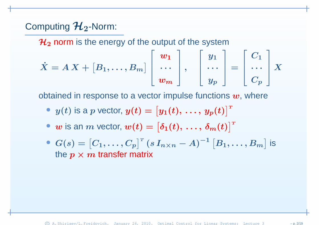
Computing H2-Norm:
H2 norm is the energy of the output of the system
X = AX +[B1, . . . , Bm
]
w1
· · ·
wm
,
y1
· · ·
yp
=
C1
· · ·
Cp
X
obtained in response to a vector impulse functions w, where
• y(t) is a p vector, y(t) =[y1(t), . . . , yp(t)
]T
• w is an m vector, w(t) =[δ1(t), . . . , δm(t)
]T
• G(s) =[C1, . . . , Cp
]T
(s In×n − A)−1 [B1, . . . , Bm
]is
the p × m transfer matrix
c© A.Shiriaev/L.Freidovich. January 26, 2010. Optimal Control for Linear Systems: Lecture 3 – p. 2/19

Computing H2-Norm:
H2 norm is the energy of the output of the system
X = AX +[B1, . . . , Bm
]
w1
· · ·
wm
,
y1
· · ·
yp
=
C1
· · ·
Cp
X
obtained in response to a vector impulse functions w, where
• y(t) is a p vector, y(t) =[y1(t), . . . , yp(t)
]T
• w is an m vector, w(t) =[δ1(t), . . . , δm(t)
]T
• G(s) =[C1, . . . , Cp
]T
(s In×n − A)−1 [B1, . . . , Bm
]is
the p × m transfer matrix
The yi(t)-component to the impulse in wj-channel is
yij(t) =
{
CieAtBj, t > 0
0, t ≤ 0
c© A.Shiriaev/L.Freidovich. January 26, 2010. Optimal Control for Linear Systems: Lecture 3 – p. 2/19

Computing H2-Norm:
H2 norm is the energy of the output of the system
X = AX +[B1, . . . , Bm
]
w1
· · ·
wm
,
y1
· · ·
yp
=
C1
· · ·
Cp
X
obtained in response to w(t) =[δ1(t), . . . , δm(t)
]T .
The yi(t)-component to the impulse in wj-channel is
yij(t) =
{
CieAtBj, t > 0
0, t ≤ 0g(t) :=
y11(t) · · · y1m(t)
· · · · · ·
yp1(t) · · · ypm(t)
The H2-norm of the system is the sum of the energies of yij(t)
∣∣G(·)
∣∣2:=
√√√√√
+∞∫
0
p∑
i=1
m∑
j=1
y2ij(t)dt =
√√√√√
+∞∫
0
trace [gT (t)g(t)] dt
c© A.Shiriaev/L.Freidovich. January 26, 2010. Optimal Control for Linear Systems: Lecture 3 – p. 2/19
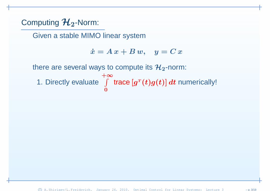
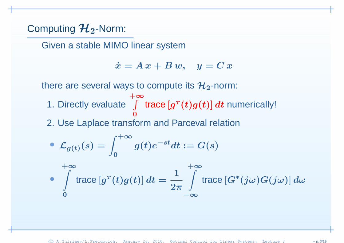
Computing H2-Norm:
Given a stable MIMO linear system
x = Ax + Bw, y = C x
there are several ways to compute its H2-norm:
1. Directly evaluate+∞∫
0
trace [gT (t)g(t)] dt numerically!
c© A.Shiriaev/L.Freidovich. January 26, 2010. Optimal Control for Linear Systems: Lecture 3 – p. 3/19
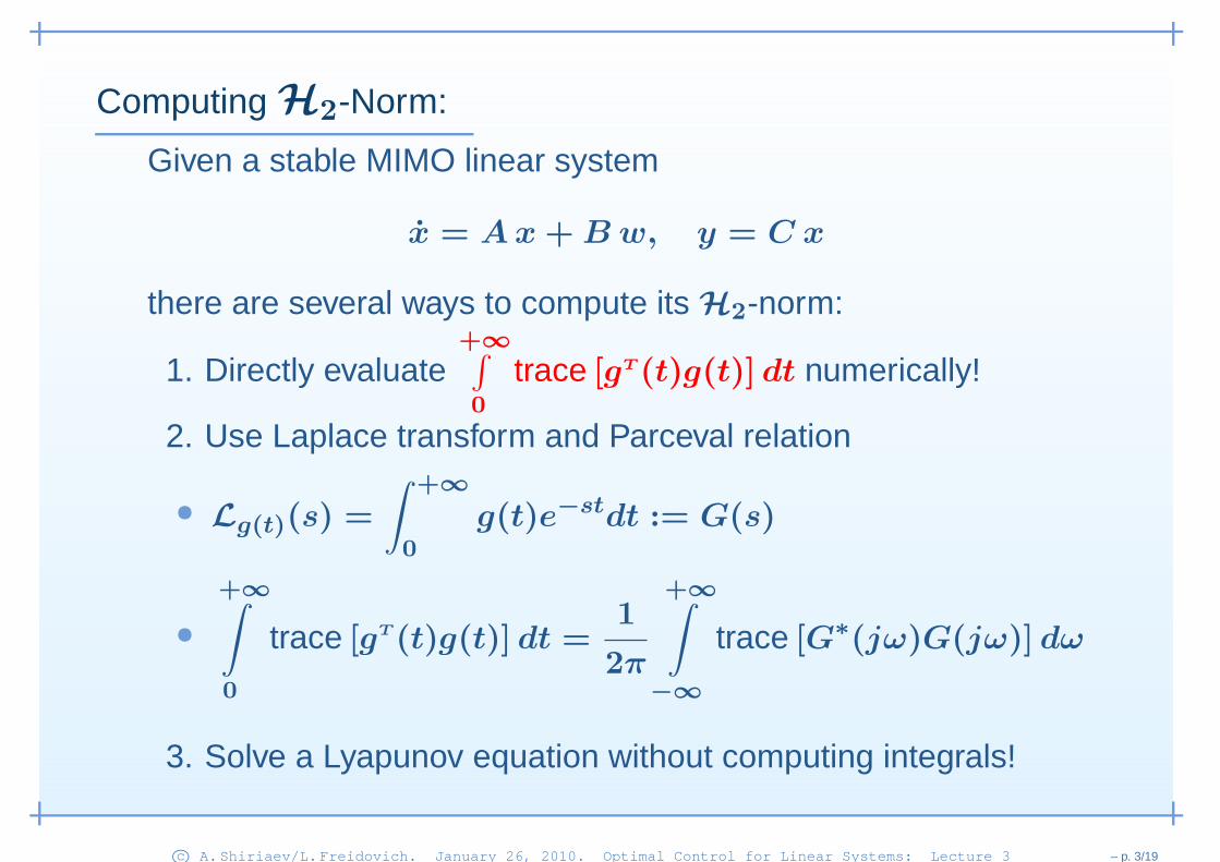
Computing H2-Norm:
Given a stable MIMO linear system
x = Ax + Bw, y = C x
there are several ways to compute its H2-norm:
1. Directly evaluate+∞∫
0
trace [gT (t)g(t)] dt numerically!
2. Use Laplace transform and Parceval relation
• Lg(t)(s) =
∫ +∞
0g(t)e−stdt := G(s)
•
+∞∫
0
trace [gT (t)g(t)] dt =1
2π
+∞∫
−∞
trace [G∗(jω)G(jω)] dω
c© A.Shiriaev/L.Freidovich. January 26, 2010. Optimal Control for Linear Systems: Lecture 3 – p. 3/19
Computing H2-Norm:
Given a stable MIMO linear system
x = Ax + Bw, y = C x
there are several ways to compute its H2-norm:
1. Directly evaluate+∞∫
0
trace [gT (t)g(t)] dt numerically!
2. Use Laplace transform and Parceval relation
• Lg(t)(s) =
∫ +∞
0g(t)e−stdt := G(s)
•
+∞∫
0
trace [gT (t)g(t)] dt =1
2π
+∞∫
−∞
trace [G∗(jω)G(jω)] dω
3. Solve a Lyapunov equation without computing integrals!
c© A.Shiriaev/L.Freidovich. January 26, 2010. Optimal Control for Linear Systems: Lecture 3 – p. 3/19
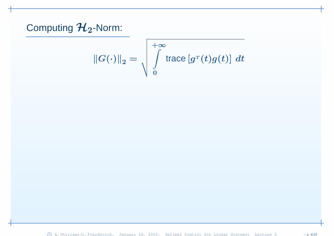
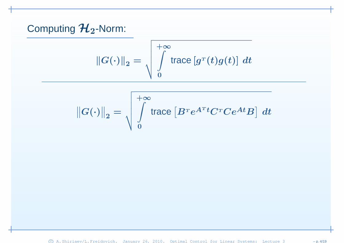
Computing H2-Norm:
‖G(·)‖2 =
√√√√√
+∞∫
0
trace [gT (t)g(t)] dt
c© A.Shiriaev/L.Freidovich. January 26, 2010. Optimal Control for Linear Systems: Lecture 3 – p. 4/19
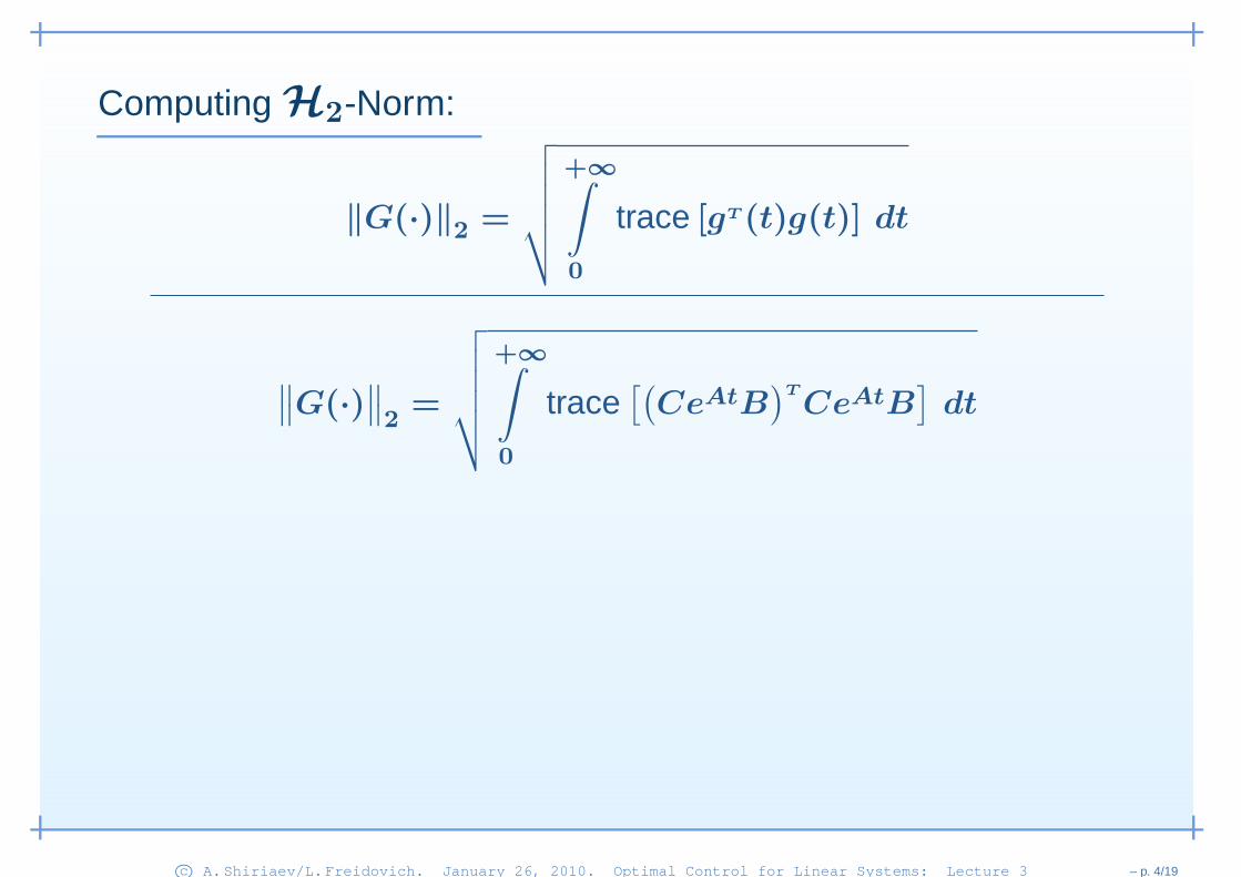
Computing H2-Norm:
‖G(·)‖2 =
√√√√√
+∞∫
0
trace [gT (t)g(t)] dt
∥∥G(·)
∥∥2=
√√√√√
+∞∫
0
trace[(CeAtB
)T
CeAtB]dt
c© A.Shiriaev/L.Freidovich. January 26, 2010. Optimal Control for Linear Systems: Lecture 3 – p. 4/19
Computing H2-Norm:
‖G(·)‖2 =
√√√√√
+∞∫
0
trace [gT (t)g(t)] dt
∥∥G(·)
∥∥2=
√√√√√
+∞∫
0
trace[BTeA
T tCTCeAtB]dt
c© A.Shiriaev/L.Freidovich. January 26, 2010. Optimal Control for Linear Systems: Lecture 3 – p. 4/19
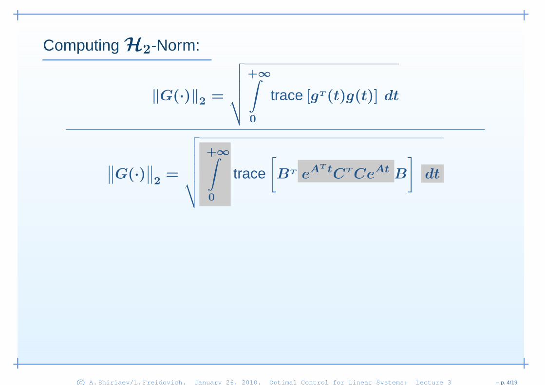
Computing H2-Norm:
‖G(·)‖2 =
√√√√√
+∞∫
0
trace [gT (t)g(t)] dt
∥∥G(·)
∥∥2=
√√√√√√
+∞∫
0
trace[
BT eAT tCTCeAt B
]
dt
c© A.Shiriaev/L.Freidovich. January 26, 2010. Optimal Control for Linear Systems: Lecture 3 – p. 4/19

Computing H2-Norm:
‖G(·)‖2 =
√√√√√
+∞∫
0
trace [gT (t)g(t)] dt
∥∥G(·)
∥∥2=
√√√√√√trace
BT
+∞∫
0
eAT tCTCeAt dt B
c© A.Shiriaev/L.Freidovich. January 26, 2010. Optimal Control for Linear Systems: Lecture 3 – p. 4/19
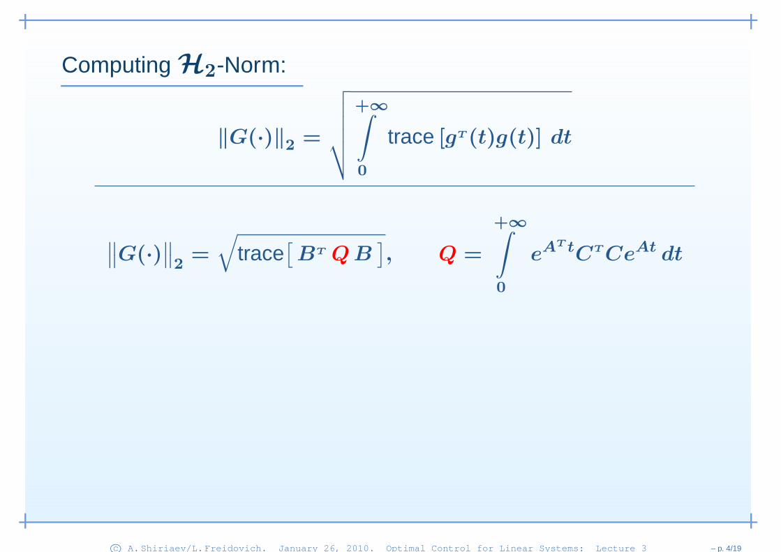
Computing H2-Norm:
‖G(·)‖2 =
√√√√√
+∞∫
0
trace [gT (t)g(t)] dt
∥∥G(·)
∥∥2=
√
trace[BT QB
], Q =
+∞∫
0
eAT tCTCeAt dt
c© A.Shiriaev/L.Freidovich. January 26, 2010. Optimal Control for Linear Systems: Lecture 3 – p. 4/19
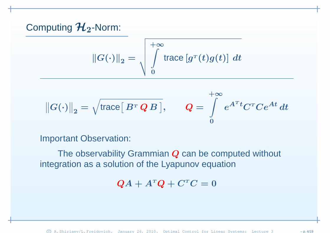
Computing H2-Norm:
‖G(·)‖2 =
√√√√√
+∞∫
0
trace [gT (t)g(t)] dt
∥∥G(·)
∥∥2=
√
trace[BT QB
], Q =
+∞∫
0
eAT tCTCeAt dt
Important Observation:
The observability Grammian Q can be computed withoutintegration as a solution of the Lyapunov equation
QA + ATQ + CTC = 0
c© A.Shiriaev/L.Freidovich. January 26, 2010. Optimal Control for Linear Systems: Lecture 3 – p. 4/19

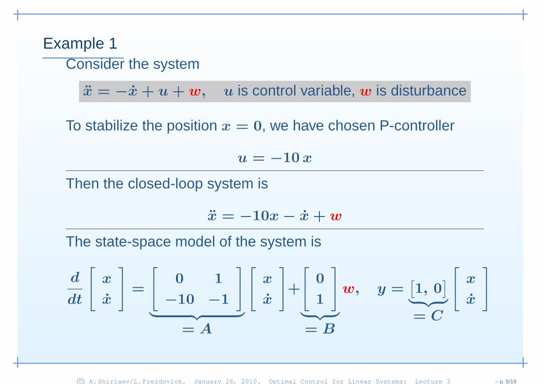
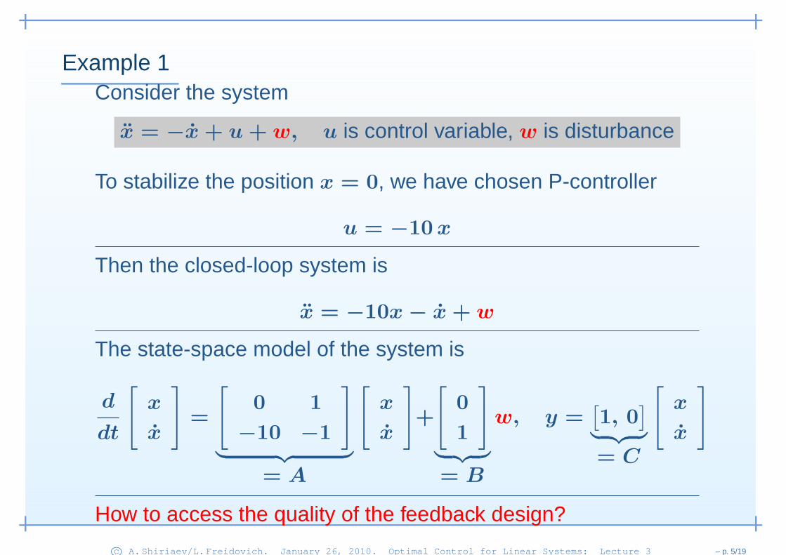
Example 1Consider the system
x = −x + u + w, u is control variable, w is disturbance
To stabilize the position x = 0, we have chosen P-controller
u = −10x
c© A.Shiriaev/L.Freidovich. January 26, 2010. Optimal Control for Linear Systems: Lecture 3 – p. 5/19

Example 1Consider the system
x = −x + u + w, u is control variable, w is disturbance
To stabilize the position x = 0, we have chosen P-controller
u = −10x
Then the closed-loop system is
x = −10x − x + w
c© A.Shiriaev/L.Freidovich. January 26, 2010. Optimal Control for Linear Systems: Lecture 3 – p. 5/19
Example 1Consider the system
x = −x + u + w, u is control variable, w is disturbance
To stabilize the position x = 0, we have chosen P-controller
u = −10x
Then the closed-loop system is
x = −10x − x + w
The state-space model of the system is
d
dt
[
x
x
]
=
[
0 1
−10 −1
]
︸ ︷︷ ︸
= A
[
x
x
]
+
[
0
1
]
︸ ︷︷ ︸
= B
w, y =[1, 0
]
︸ ︷︷ ︸
= C
[
x
x
]
How to access the quality of the feedback design?
c© A.Shiriaev/L.Freidovich. January 26, 2010. Optimal Control for Linear Systems: Lecture 3 – p. 5/19
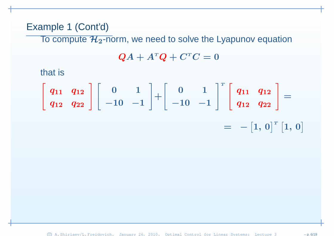
Example 1 (Cont’d)To compute H2-norm, we need to solve the Lyapunov equation
QA + ATQ + CTC = 0
that is[
q11 q12
q12 q22
] [
0 1
−10 −1
]
+
[
0 1
−10 −1
]T[
q11 q12
q12 q22
]
=
= −[1, 0
]T[1, 0
]
c© A.Shiriaev/L.Freidovich. January 26, 2010. Optimal Control for Linear Systems: Lecture 3 – p. 6/19
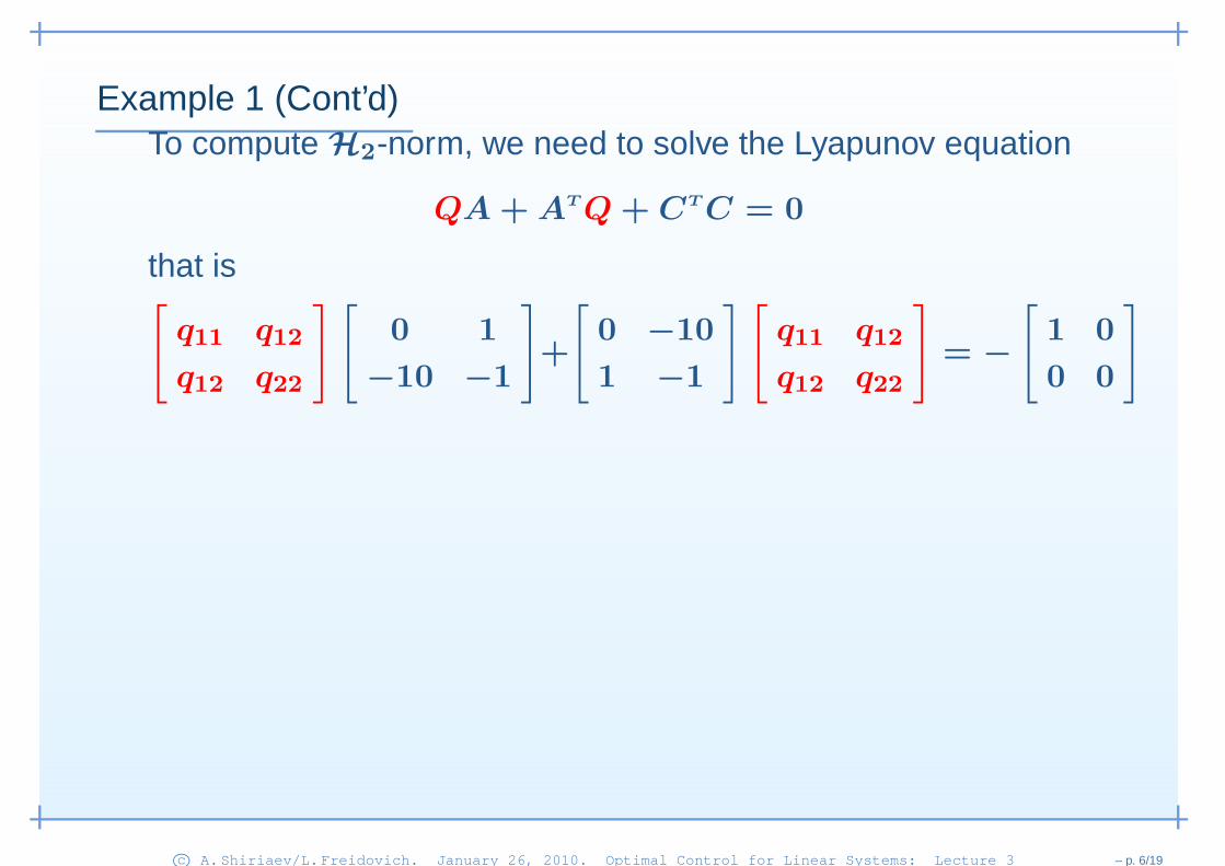
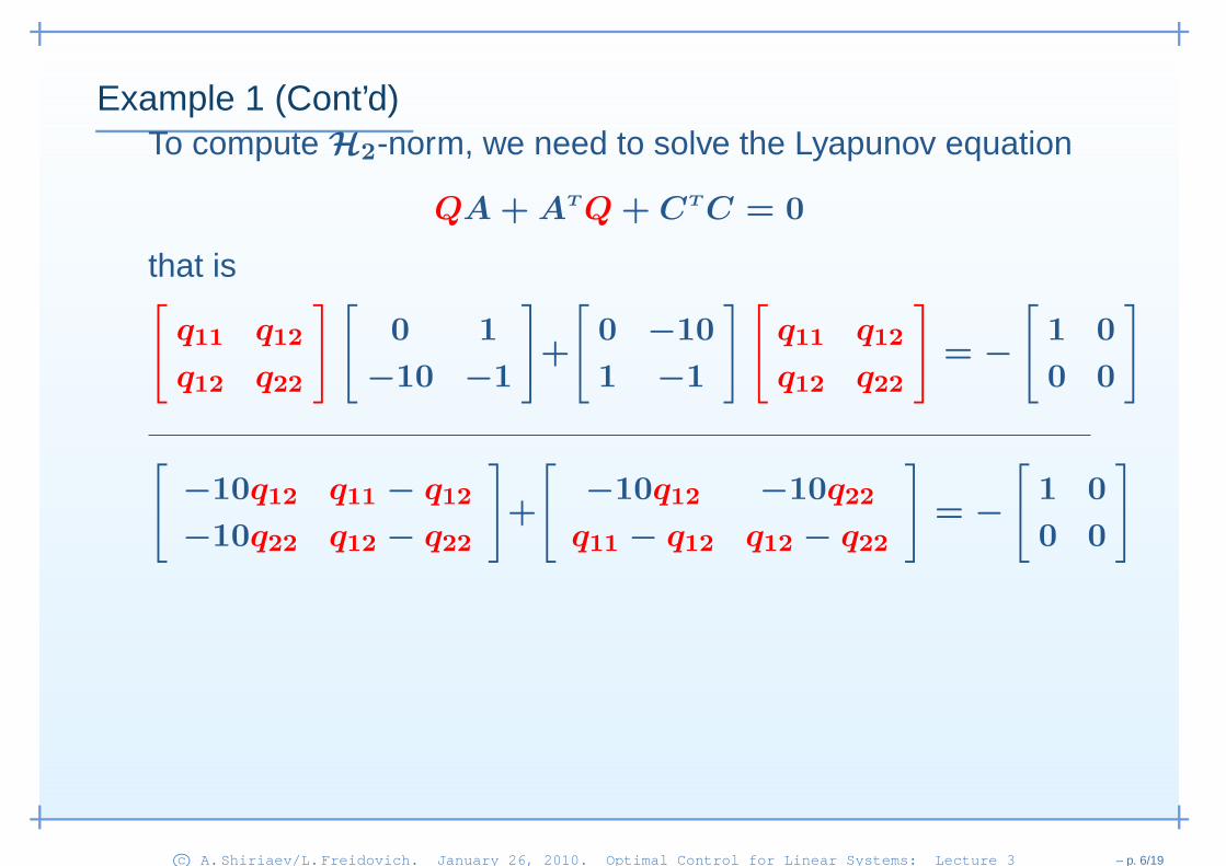
Example 1 (Cont’d)To compute H2-norm, we need to solve the Lyapunov equation
QA + ATQ + CTC = 0
that is[
q11 q12
q12 q22
] [
0 1
−10 −1
]
+
[
0 −10
1 −1
] [
q11 q12
q12 q22
]
= −
[
1 0
0 0
]
c© A.Shiriaev/L.Freidovich. January 26, 2010. Optimal Control for Linear Systems: Lecture 3 – p. 6/19
Example 1 (Cont’d)To compute H2-norm, we need to solve the Lyapunov equation
QA + ATQ + CTC = 0
that is[
q11 q12
q12 q22
] [
0 1
−10 −1
]
+
[
0 −10
1 −1
] [
q11 q12
q12 q22
]
= −
[
1 0
0 0
]
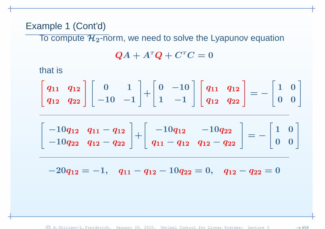
[
−10q12 q11 − q12
−10q22 q12 − q22
]
+
[
−10q12 −10q22
q11 − q12 q12 − q22
]
= −
[
1 0
0 0
]
c© A.Shiriaev/L.Freidovich. January 26, 2010. Optimal Control for Linear Systems: Lecture 3 – p. 6/19
Example 1 (Cont’d)To compute H2-norm, we need to solve the Lyapunov equation
QA + ATQ + CTC = 0
that is[
q11 q12
q12 q22
] [
0 1
−10 −1
]
+
[
0 −10
1 −1
] [
q11 q12
q12 q22
]
= −
[
1 0
0 0
]
[
−10q12 q11 − q12
−10q22 q12 − q22
]
+
[
−10q12 −10q22
q11 − q12 q12 − q22
]
= −
[
1 0
0 0
]
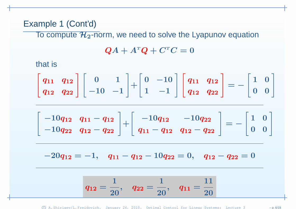
−20q12 = −1, q11 − q12 − 10q22 = 0, q12 − q22 = 0
c© A.Shiriaev/L.Freidovich. January 26, 2010. Optimal Control for Linear Systems: Lecture 3 – p. 6/19
Example 1 (Cont’d)To compute H2-norm, we need to solve the Lyapunov equation
QA + ATQ + CTC = 0
that is[
q11 q12
q12 q22
] [
0 1
−10 −1
]
+
[
0 −10
1 −1
] [
q11 q12
q12 q22
]
= −
[
1 0
0 0
]
[
−10q12 q11 − q12
−10q22 q12 − q22
]
+
[
−10q12 −10q22
q11 − q12 q12 − q22
]
= −
[
1 0
0 0
]
−20q12 = −1, q11 − q12 − 10q22 = 0, q12 − q22 = 0
q12 =1
20, q22 =
1
20, q11 =
11
20
c© A.Shiriaev/L.Freidovich. January 26, 2010. Optimal Control for Linear Systems: Lecture 3 – p. 6/19
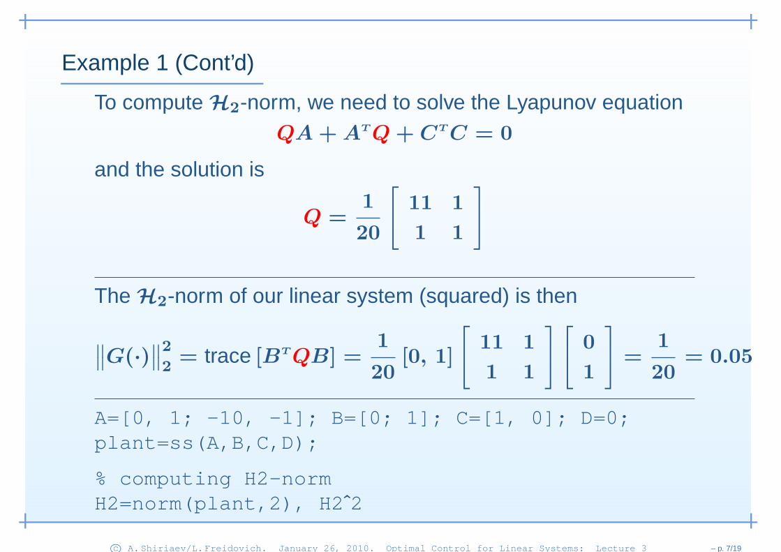
Example 1 (Cont’d)
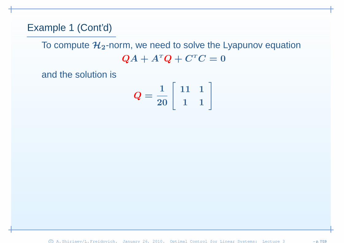
To compute H2-norm, we need to solve the Lyapunov equationQA + ATQ + CTC = 0
and the solution is
Q =1
20
[
11 1
1 1
]
c© A.Shiriaev/L.Freidovich. January 26, 2010. Optimal Control for Linear Systems: Lecture 3 – p. 7/19

Example 1 (Cont’d)
To compute H2-norm, we need to solve the Lyapunov equationQA + ATQ + CTC = 0
and the solution is
Q =1
20
[
11 1
1 1
]
The H2-norm of our linear system (squared) is then
∥∥G(·)
∥∥2
2= trace [BTQB] =
1
20[0, 1]
[
11 1
1 1
] [
0
1
]
=1
20= 0.05
c© A.Shiriaev/L.Freidovich. January 26, 2010. Optimal Control for Linear Systems: Lecture 3 – p. 7/19
Example 1 (Cont’d)
To compute H2-norm, we need to solve the Lyapunov equationQA + ATQ + CTC = 0
and the solution is
Q =1
20
[
11 1
1 1
]
The H2-norm of our linear system (squared) is then
∥∥G(·)
∥∥2
2= trace [BTQB] =
1
20[0, 1]
[
11 1
1 1
] [
0
1
]
=1
20= 0.05
A=[0, 1; -10, -1]; B=[0; 1]; C=[1, 0]; D=0;plant=ss(A,B,C,D);
% computing H2-normH2=norm(plant,2), H2 2
c© A.Shiriaev/L.Freidovich. January 26, 2010. Optimal Control for Linear Systems: Lecture 3 – p. 7/19
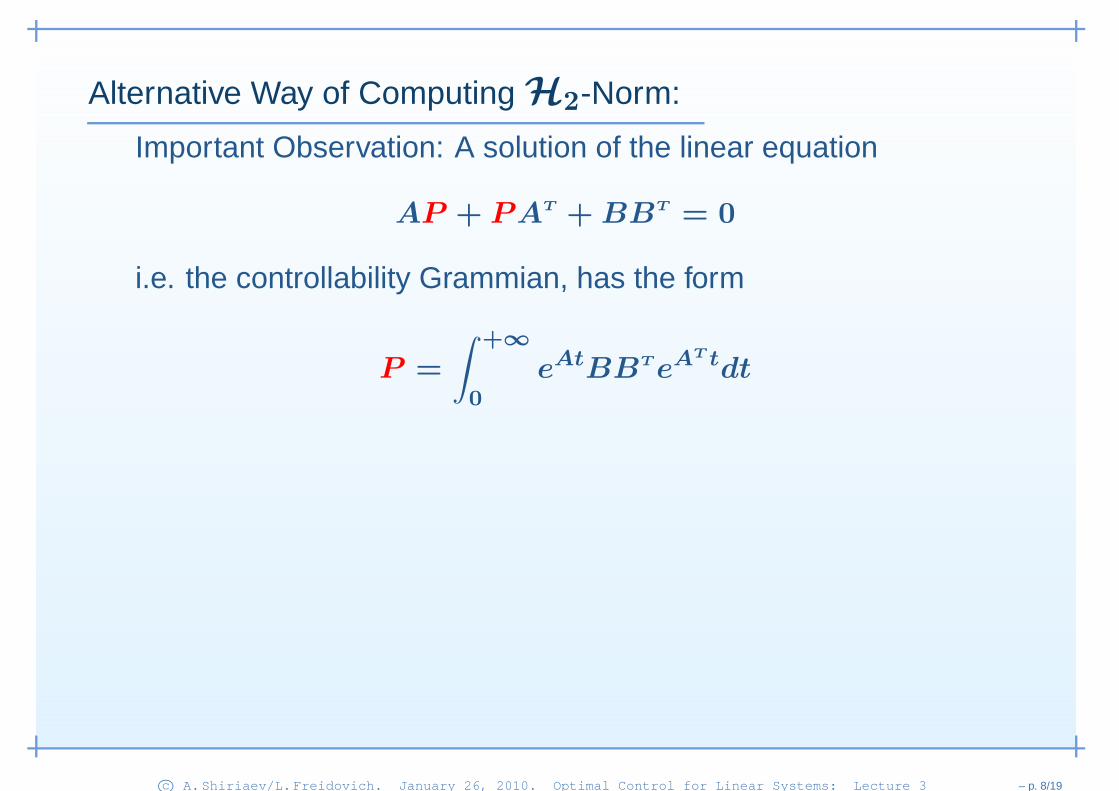
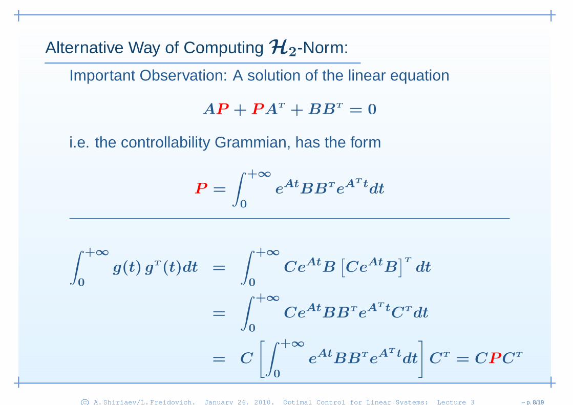
Alternative Way of Computing H2-Norm:
Important Observation: A solution of the linear equation
AP + PAT + BBT = 0
i.e. the controllability Grammian, has the form
P =
∫ +∞
0eAtBBTeA
T tdt
c© A.Shiriaev/L.Freidovich. January 26, 2010. Optimal Control for Linear Systems: Lecture 3 – p. 8/19
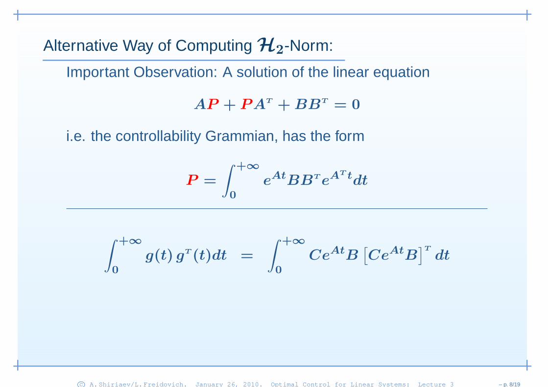
Alternative Way of Computing H2-Norm:
Important Observation: A solution of the linear equation
AP + PAT + BBT = 0
i.e. the controllability Grammian, has the form
P =
∫ +∞
0eAtBBTeA
T tdt
∫ +∞
0g(t) gT (t)dt =
∫ +∞
0CeAtB
[CeAtB
]T
dt
c© A.Shiriaev/L.Freidovich. January 26, 2010. Optimal Control for Linear Systems: Lecture 3 – p. 8/19

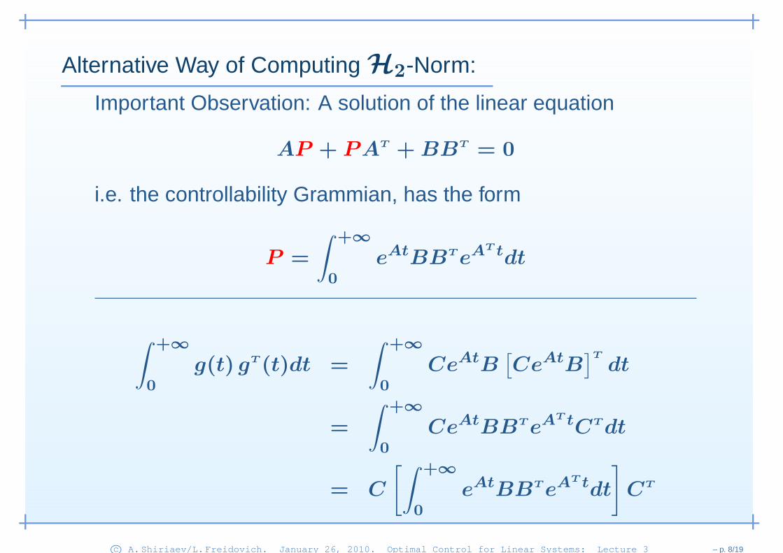
Alternative Way of Computing H2-Norm:
Important Observation: A solution of the linear equation
AP + PAT + BBT = 0
i.e. the controllability Grammian, has the form
P =
∫ +∞
0eAtBBTeA
T tdt
∫ +∞
0g(t) gT (t)dt =
∫ +∞
0CeAtB
[CeAtB
]T
dt
=
∫ +∞
0CeAtBBTeA
T tCTdt
c© A.Shiriaev/L.Freidovich. January 26, 2010. Optimal Control for Linear Systems: Lecture 3 – p. 8/19
Alternative Way of Computing H2-Norm:
Important Observation: A solution of the linear equation
AP + PAT + BBT = 0
i.e. the controllability Grammian, has the form
P =
∫ +∞
0eAtBBTeA
T tdt
∫ +∞
0g(t) gT (t)dt =
∫ +∞
0CeAtB
[CeAtB
]T
dt
=
∫ +∞
0CeAtBBTeA
T tCTdt
= C
[∫ +∞
0eAtBBTeA
T tdt
]
CT
c© A.Shiriaev/L.Freidovich. January 26, 2010. Optimal Control for Linear Systems: Lecture 3 – p. 8/19
Alternative Way of Computing H2-Norm:
Important Observation: A solution of the linear equation
AP + PAT + BBT = 0
i.e. the controllability Grammian, has the form
P =
∫ +∞
0eAtBBTeA
T tdt
∫ +∞
0g(t) gT (t)dt =
∫ +∞
0CeAtB
[CeAtB
]T
dt
=
∫ +∞
0CeAtBBTeA
T tCTdt
= C
[∫ +∞
0eAtBBTeA
T tdt
]
CT = CPCT
c© A.Shiriaev/L.Freidovich. January 26, 2010. Optimal Control for Linear Systems: Lecture 3 – p. 8/19
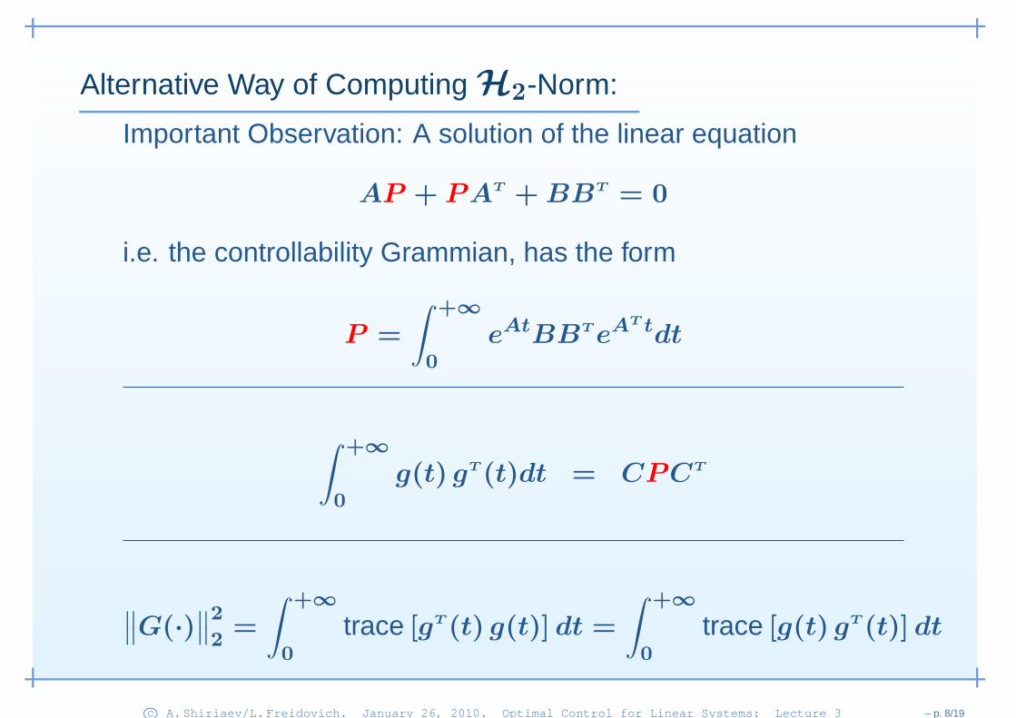
Alternative Way of Computing H2-Norm:
Important Observation: A solution of the linear equation
AP + PAT + BBT = 0
i.e. the controllability Grammian, has the form
P =
∫ +∞
0eAtBBTeA
T tdt
∫ +∞
0g(t) gT (t)dt = CPCT
∥∥G(·)
∥∥2
2=
∫ +∞
0trace [gT (t) g(t)] dt =
∫ +∞
0trace [g(t) gT (t)] dt
c© A.Shiriaev/L.Freidovich. January 26, 2010. Optimal Control for Linear Systems: Lecture 3 – p. 8/19
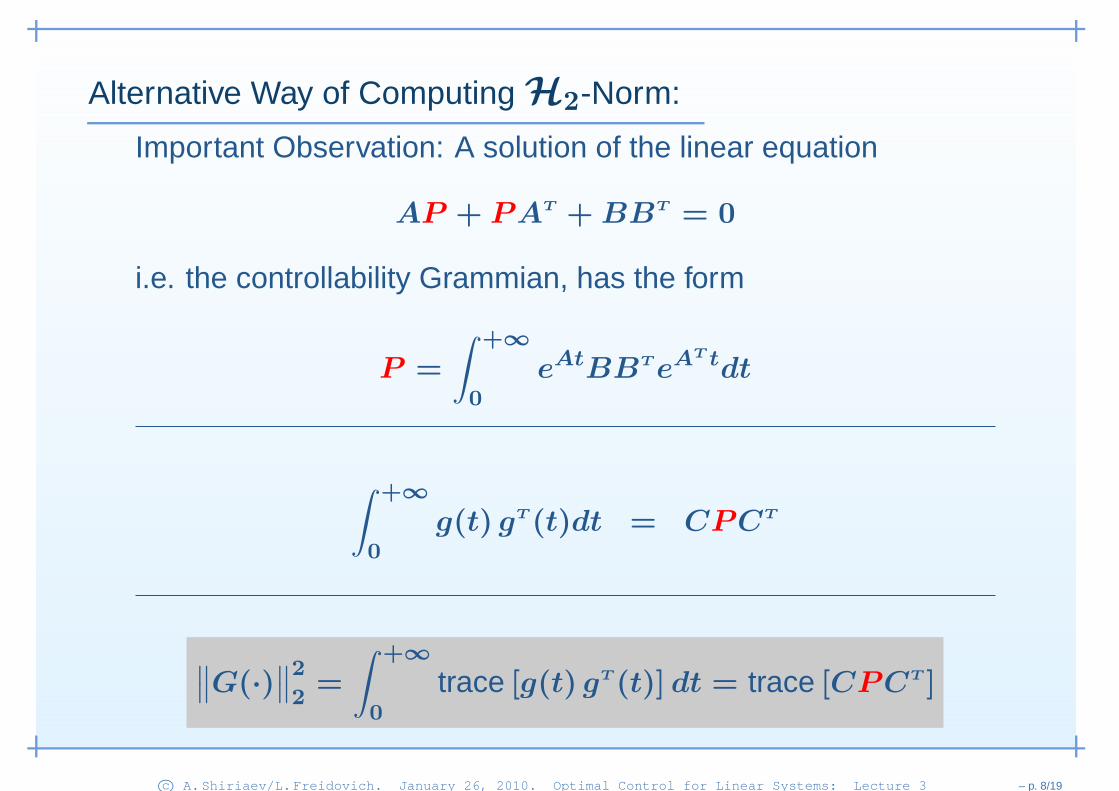
Alternative Way of Computing H2-Norm:
Important Observation: A solution of the linear equation
AP + PAT + BBT = 0
i.e. the controllability Grammian, has the form
P =
∫ +∞
0eAtBBTeA
T tdt
∫ +∞
0g(t) gT (t)dt = CPCT
∥∥G(·)
∥∥2
2=
∫ +∞
0trace [g(t) gT (t)] dt = trace [CPCT ]
c© A.Shiriaev/L.Freidovich. January 26, 2010. Optimal Control for Linear Systems: Lecture 3 – p. 8/19

Lecture 3: How to Compute H2 and H∞-Norms
• Computing H2-Norm for Stable Linear Systems
• Computing H∞-Norm for Stable Linear Systems
c© A.Shiriaev/L.Freidovich. January 26, 2010. Optimal Control for Linear Systems: Lecture 3 – p. 9/19
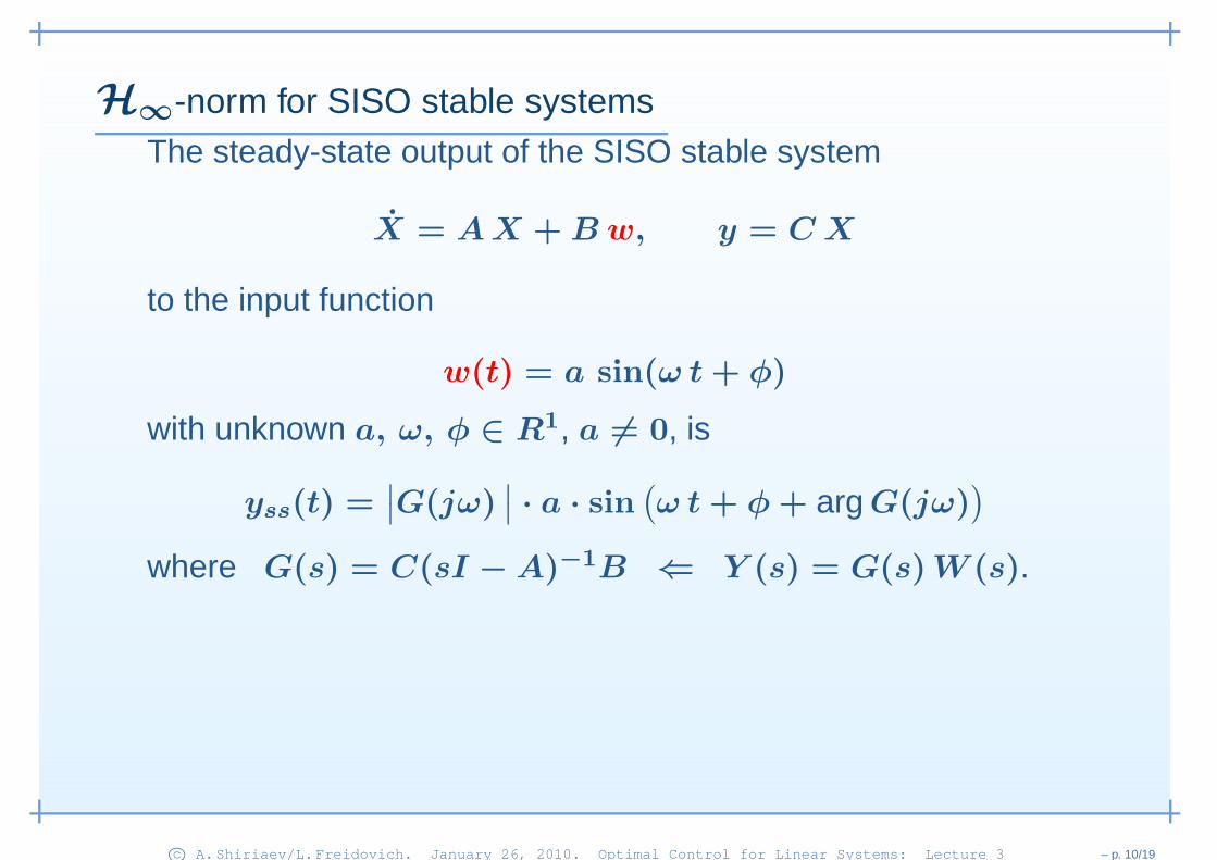
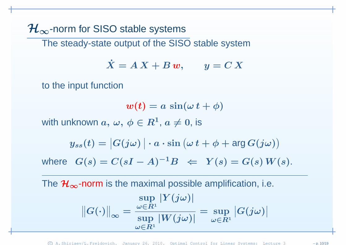
H∞-norm for SISO stable systemsThe steady-state output of the SISO stable system
X = AX + Bw, y = C X
to the input function
w(t) = a sin(ω t + φ)
with unknown a, ω, φ ∈ R1, a 6= 0, is
yss(t) =∣∣G(jω)
∣∣ · a · sin
(ω t + φ + argG(jω)
)
where G(s) = C(sI − A)−1B ⇐ Y (s) = G(s)W (s).
c© A.Shiriaev/L.Freidovich. January 26, 2010. Optimal Control for Linear Systems: Lecture 3 – p. 10/19
H∞-norm for SISO stable systemsThe steady-state output of the SISO stable system
X = AX + Bw, y = C X
to the input function
w(t) = a sin(ω t + φ)
with unknown a, ω, φ ∈ R1, a 6= 0, is
yss(t) =∣∣G(jω)
∣∣ · a · sin
(ω t + φ + argG(jω)
)
where G(s) = C(sI − A)−1B ⇐ Y (s) = G(s)W (s).
The H∞-norm is the maximal possible amplification, i.e.
∥∥G(·)
∥∥∞
=
supω∈R1
|Y (jω)|
supω∈R1
|W (jω)|= sup
ω∈R1
∣∣G(jω)
∣∣
c© A.Shiriaev/L.Freidovich. January 26, 2010. Optimal Control for Linear Systems: Lecture 3 – p. 10/19
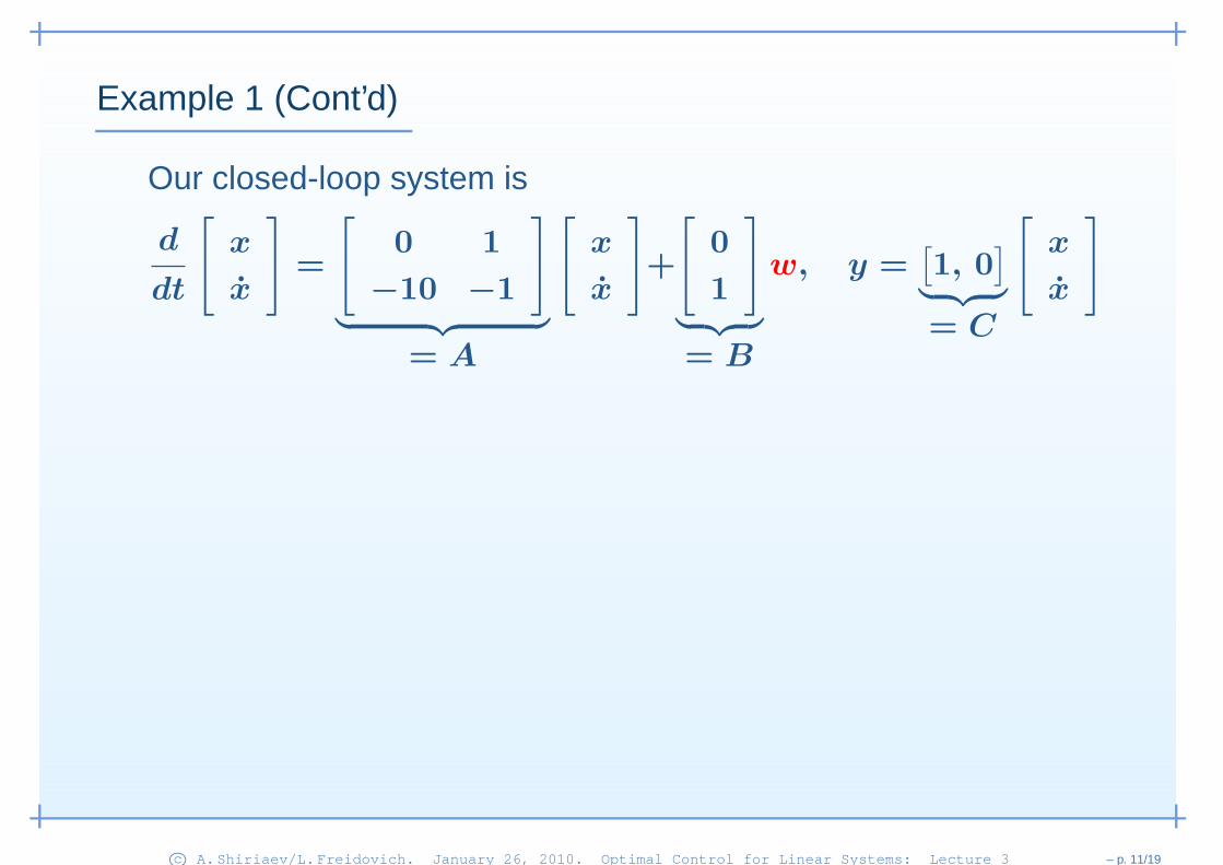
Example 1 (Cont’d)
Our closed-loop system is
d
dt
[
x
x
]
=
[
0 1
−10 −1
]
︸ ︷︷ ︸
= A
[
x
x
]
+
[
0
1
]
︸ ︷︷ ︸
= B
w, y =[1, 0
]
︸ ︷︷ ︸
= C
[
x
x
]
c© A.Shiriaev/L.Freidovich. January 26, 2010. Optimal Control for Linear Systems: Lecture 3 – p. 11/19
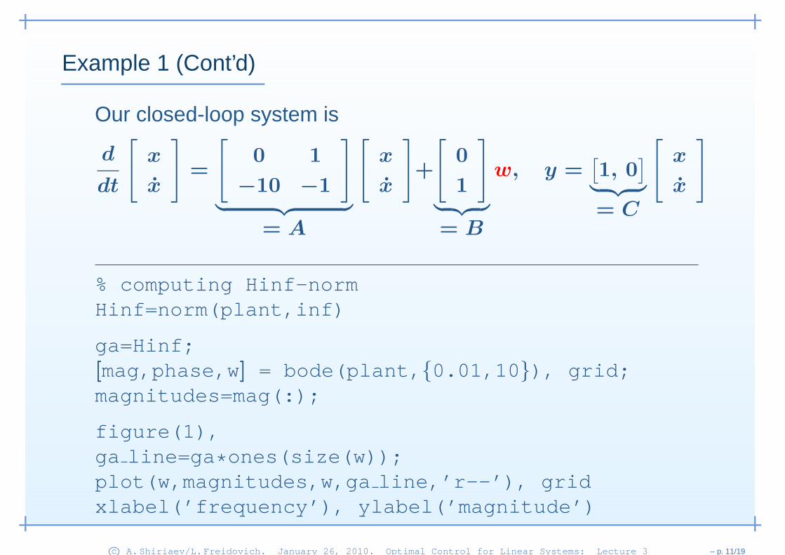
Example 1 (Cont’d)
Our closed-loop system is
d
dt
[
x
x
]
=
[
0 1
−10 −1
]
︸ ︷︷ ︸
= A
[
x
x
]
+
[
0
1
]
︸ ︷︷ ︸
= B
w, y =[1, 0
]
︸ ︷︷ ︸
= C
[
x
x
]
% computing Hinf-normHinf=norm(plant,inf)
ga=Hinf;[mag,phase,w] = bode(plant,{0.01,10}), grid;magnitudes=mag(:);
figure(1),ga line=ga*ones(size(w));plot(w,magnitudes,w,ga line,’r--’), gridxlabel(’frequency’), ylabel(’magnitude’)
c© A.Shiriaev/L.Freidovich. January 26, 2010. Optimal Control for Linear Systems: Lecture 3 – p. 11/19
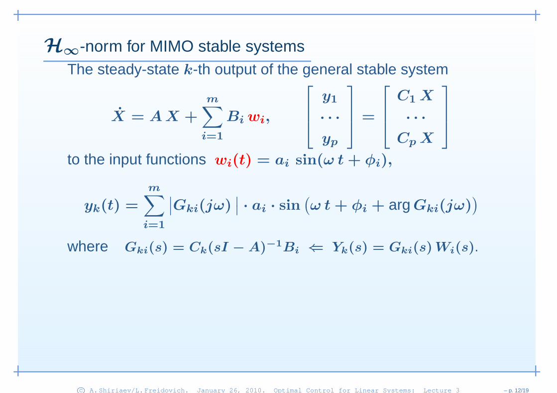
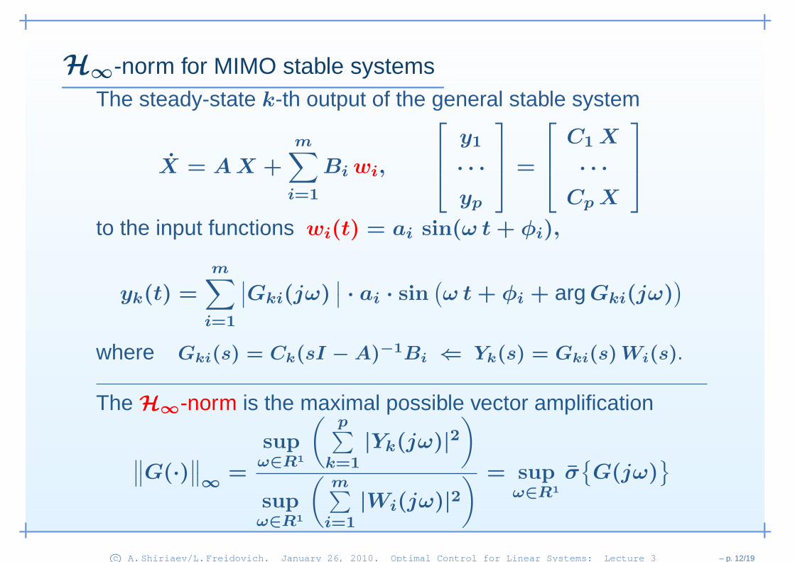
H∞-norm for MIMO stable systemsThe steady-state k-th output of the general stable system
X = AX +
m∑
i=1
Bi wi,
y1
· · ·
yp
=
C1 X
· · ·
Cp X
to the input functions wi(t) = ai sin(ω t + φi),
yk(t) =
m∑
i=1
∣∣Gki(jω)
∣∣ · ai · sin
(ω t + φi + argGki(jω)
)
where Gki(s) = Ck(sI − A)−1Bi ⇐ Yk(s) = Gki(s)Wi(s).
c© A.Shiriaev/L.Freidovich. January 26, 2010. Optimal Control for Linear Systems: Lecture 3 – p. 12/19
H∞-norm for MIMO stable systemsThe steady-state k-th output of the general stable system
X = AX +
m∑
i=1
Bi wi,
y1
· · ·
yp
=
C1 X
· · ·
Cp X
to the input functions wi(t) = ai sin(ω t + φi),
yk(t) =
m∑
i=1
∣∣Gki(jω)
∣∣ · ai · sin
(ω t + φi + argGki(jω)
)
where Gki(s) = Ck(sI − A)−1Bi ⇐ Yk(s) = Gki(s)Wi(s).
The H∞-norm is the maximal possible vector amplification
∥∥G(·)
∥∥∞
=
supω∈R1
(p∑
k=1
|Yk(jω)|2)
supω∈R1
(m∑
i=1
|Wi(jω)|2) = sup
ω∈R1
σ{G(jω)
}
c© A.Shiriaev/L.Freidovich. January 26, 2010. Optimal Control for Linear Systems: Lecture 3 – p. 12/19

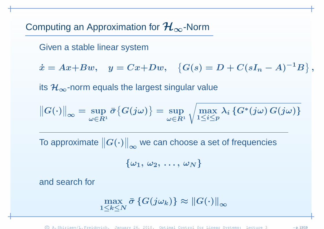
Computing an Approximation for H∞-Norm
Given a stable linear system
x = Ax+Bw, y = Cx+Dw,{G(s) = D + C(sIn − A)−1B
},
its H∞-norm equals the largest singular value
∥∥G(·)
∥∥∞
= supω∈R1
σ{G(jω)
}= sup
ω∈R1
√
max1≤i≤p
λi {G∗(jω)G(jω)}
c© A.Shiriaev/L.Freidovich. January 26, 2010. Optimal Control for Linear Systems: Lecture 3 – p. 13/19
Computing an Approximation for H∞-Norm
Given a stable linear system
x = Ax+Bw, y = Cx+Dw,{G(s) = D + C(sIn − A)−1B
},
its H∞-norm equals the largest singular value
∥∥G(·)
∥∥∞
= supω∈R1
σ{G(jω)
}= sup
ω∈R1
√
max1≤i≤p
λi {G∗(jω)G(jω)}
To approximate∥∥G(·)
∥∥∞
we can choose a set of frequencies
{ω1, ω2, . . . , ωN}
and search for
max1≤k≤N
σ {G(jωk)} ≈ ‖G(·)‖∞
c© A.Shiriaev/L.Freidovich. January 26, 2010. Optimal Control for Linear Systems: Lecture 3 – p. 13/19
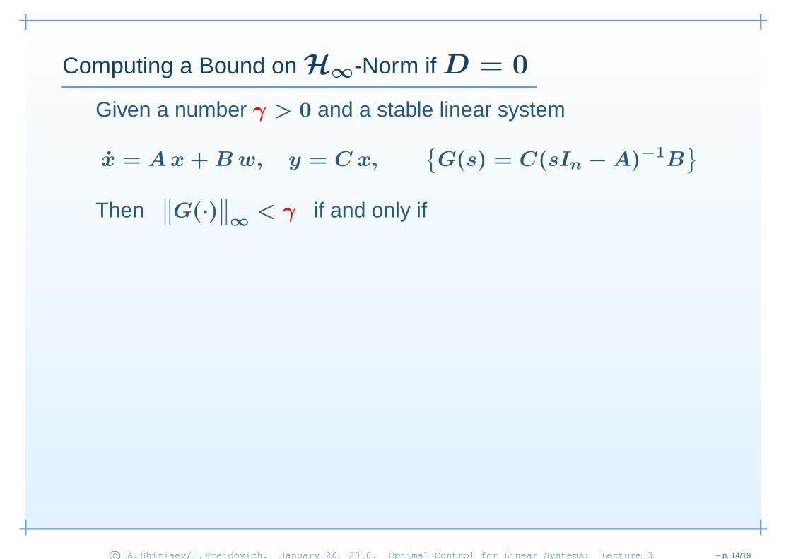
Computing a Bound on H∞-Norm if D = 0
Given a number γ > 0 and a stable linear system
x = Ax + Bw, y = C x,{G(s) = C(sIn − A)−1B
}
Then∥∥G(·)
∥∥∞
< γ if and only if
c© A.Shiriaev/L.Freidovich. January 26, 2010. Optimal Control for Linear Systems: Lecture 3 – p. 14/19
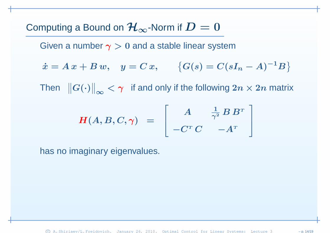
Computing a Bound on H∞-Norm if D = 0
Given a number γ > 0 and a stable linear system
x = Ax + Bw, y = C x,{G(s) = C(sIn − A)−1B
}
Then∥∥G(·)
∥∥∞
< γ if and only if the following 2n× 2n matrix
H(A,B,C, γ) =
A 1
γ2BBT
−CT C −AT
has no imaginary eigenvalues.
c© A.Shiriaev/L.Freidovich. January 26, 2010. Optimal Control for Linear Systems: Lecture 3 – p. 14/19
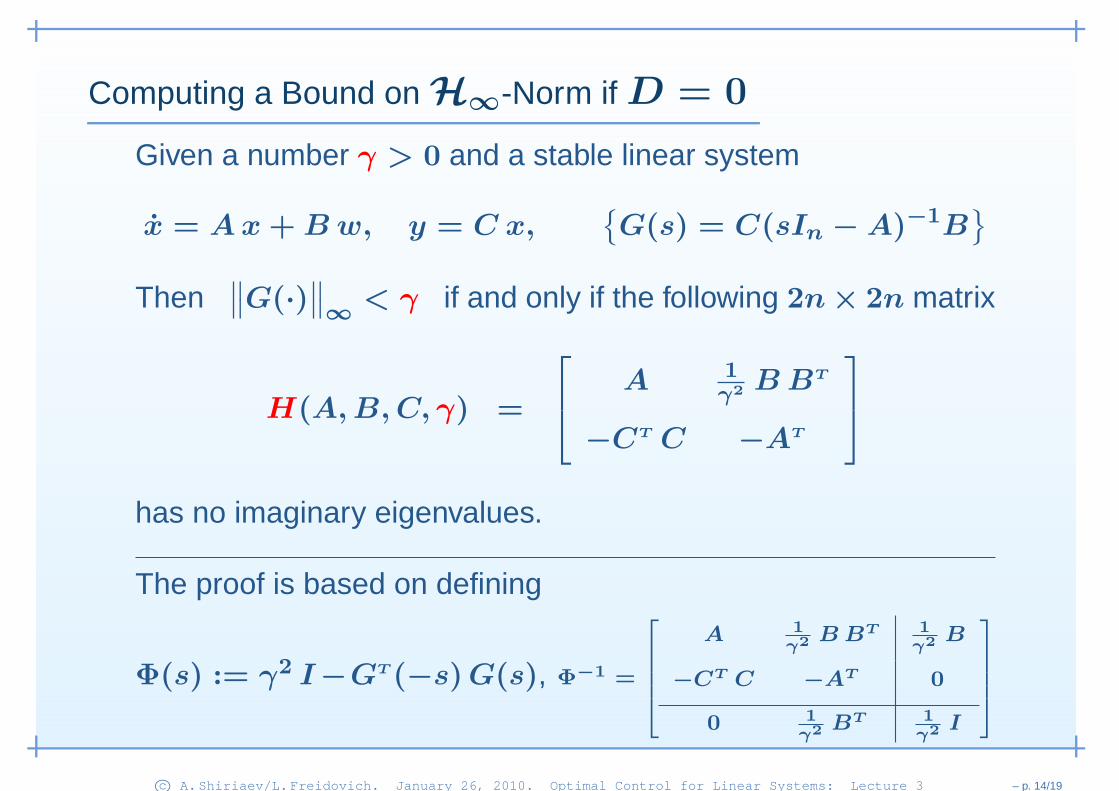
Computing a Bound on H∞-Norm if D = 0
Given a number γ > 0 and a stable linear system
x = Ax + Bw, y = C x,{G(s) = C(sIn − A)−1B
}
Then∥∥G(·)
∥∥∞
< γ if and only if the following 2n× 2n matrix
H(A,B,C, γ) =
A 1
γ2BBT
−CT C −AT
has no imaginary eigenvalues.
The proof is based on defining
Φ(s) := γ2 I−GT (−s)G(s), Φ−1 =
A 1
γ2B BT 1
γ2B
−CT C −AT 0
0 1
γ2BT 1
γ2I
c© A.Shiriaev/L.Freidovich. January 26, 2010. Optimal Control for Linear Systems: Lecture 3 – p. 14/19

Computing a Bound on H∞-Norm if D = 0
Given a number γ > 0 and a stable linear system
x = Ax + Bw, y = C x,{G(s) = C(sIn − A)−1B
}
Then∥∥G(·)
∥∥∞
< γ if and only if the following 2n× 2n matrix
H(A,B,C, γ) =
A 1
γ2BBT
−CT C −AT
has no imaginary eigenvalues.
The proof is based on defining
Φ(s) := γ2 I − GT (−s)G(s)
and using the fact that∥∥G(·)
∥∥∞
< γ ⇔ Φ(jω) > 0 (positive
definite) for ω ∈ R1 ⇔ Φ−1(jω) has no imaginary poles.
c© A.Shiriaev/L.Freidovich. January 26, 2010. Optimal Control for Linear Systems: Lecture 3 – p. 14/19
Computing a Lower Bound on H∞-Norm
Given a number γ > 0 and a stable linear system
x = Ax+Bw, y = Cx+Dw,{G(s) = D + C(sIn − A)−1B
}
Then |G(·)|∞ < γ if and only if
c© A.Shiriaev/L.Freidovich. January 26, 2010. Optimal Control for Linear Systems: Lecture 3 – p. 15/19
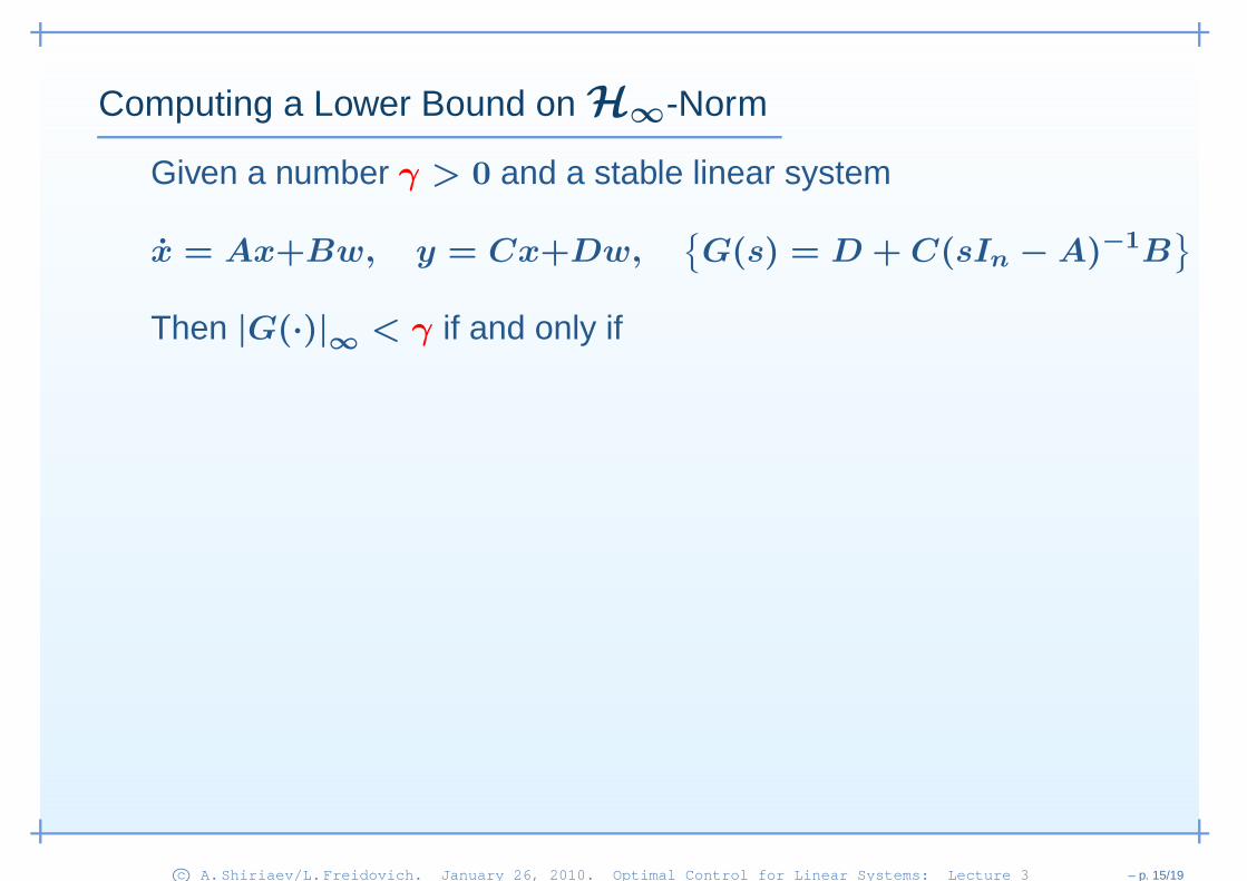
Computing a Lower Bound on H∞-Norm
Given a number γ > 0 and a stable linear system
x = Ax+Bw, y = Cx+Dw,{G(s) = D + C(sIn − A)−1B
}
Then |G(·)|∞ < γ if and only if
• σ{D}< γ;
c© A.Shiriaev/L.Freidovich. January 26, 2010. Optimal Control for Linear Systems: Lecture 3 – p. 15/19
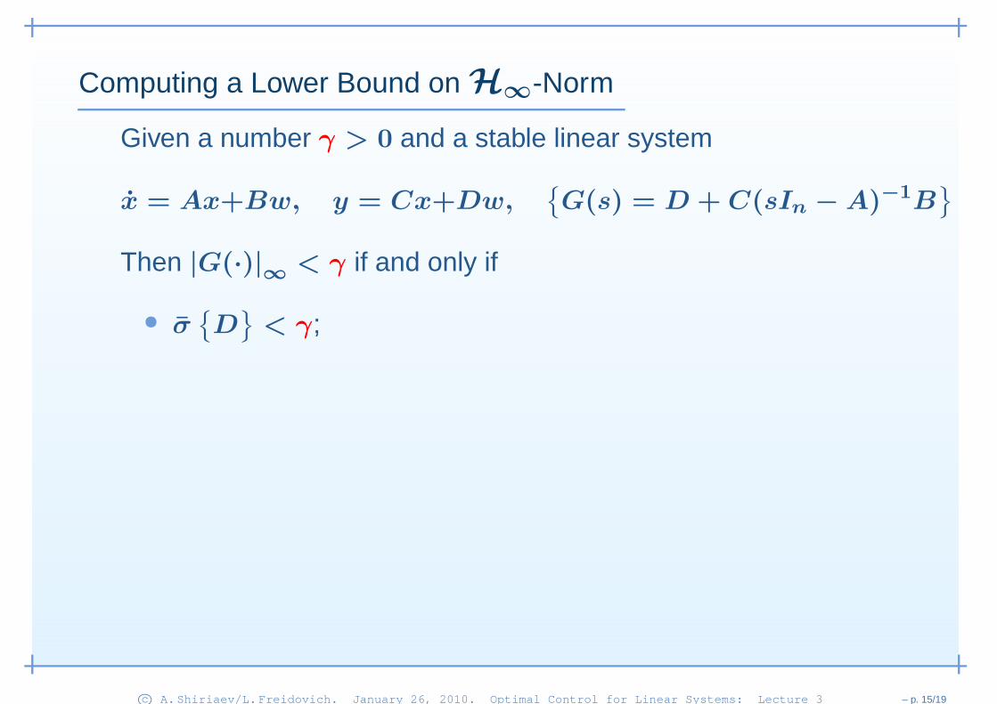
Computing a Lower Bound on H∞-Norm
Given a number γ > 0 and a stable linear system
x = Ax+Bw, y = Cx+Dw,{G(s) = D + C(sIn − A)−1B
}
Then |G(·)|∞ < γ if and only if
• σ{D}< γ;
• The following 2n × 2n matrix H = H(A,B,C,D, γ) hasno imaginary eigenvalues
c© A.Shiriaev/L.Freidovich. January 26, 2010. Optimal Control for Linear Systems: Lecture 3 – p. 15/19
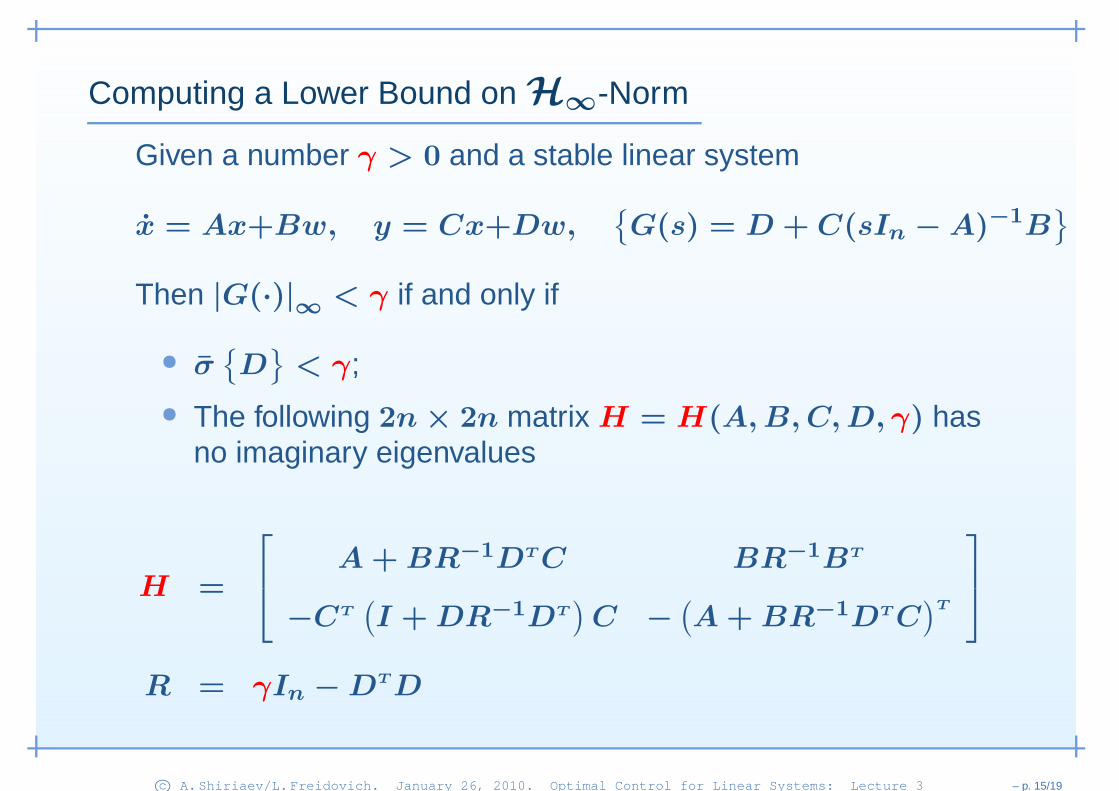
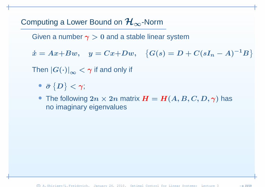
Computing a Lower Bound on H∞-Norm
Given a number γ > 0 and a stable linear system
x = Ax+Bw, y = Cx+Dw,{G(s) = D + C(sIn − A)−1B
}
Then |G(·)|∞ < γ if and only if
• σ{D}< γ;
• The following 2n × 2n matrix H = H(A,B,C,D, γ) hasno imaginary eigenvalues
H =
A + BR−1DTC BR−1BT
−CT
(I + DR−1DT
)C −
(A + BR−1DTC
)T
R = γIn − DTD
c© A.Shiriaev/L.Freidovich. January 26, 2010. Optimal Control for Linear Systems: Lecture 3 – p. 15/19
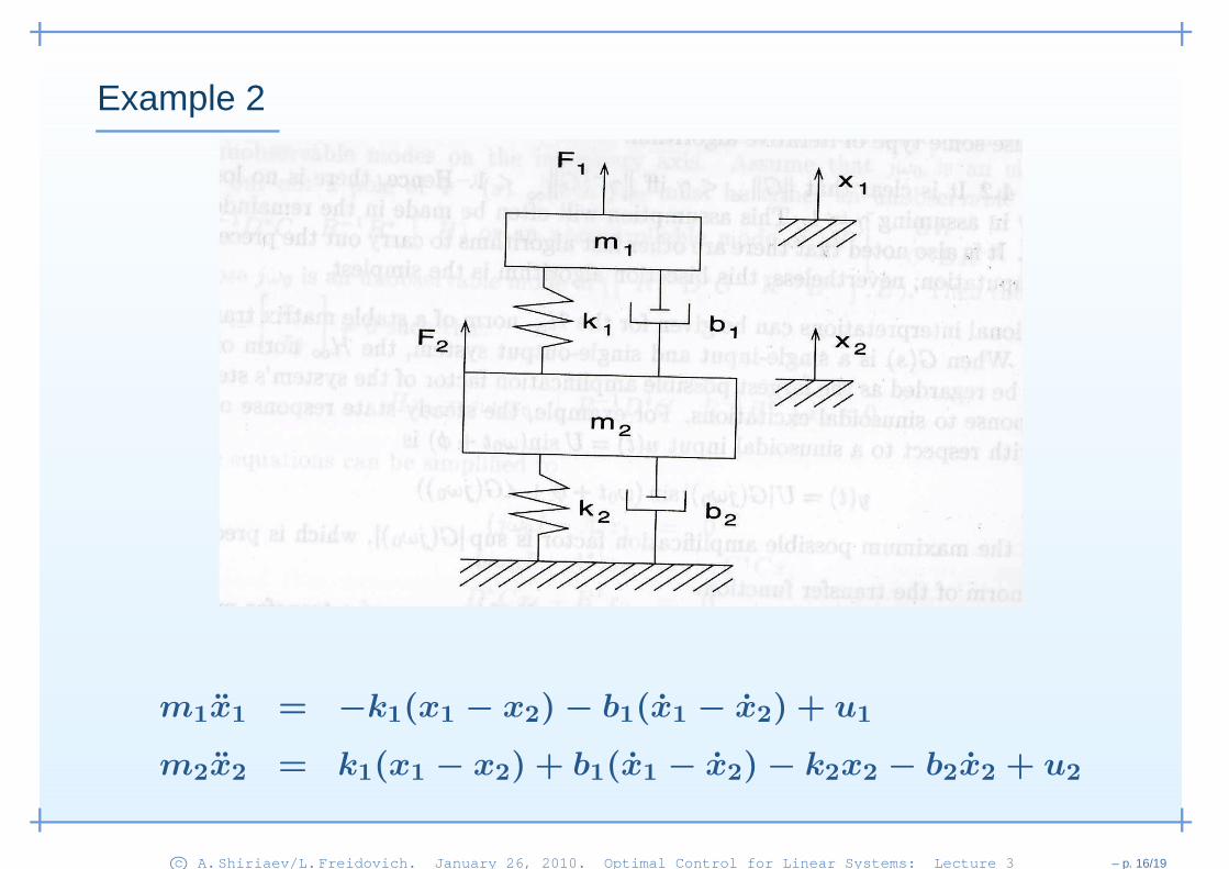
Example 2
m1x1 = −k1(x1 − x2) − b1(x1 − x2) + u1
m2x2 = k1(x1 − x2) + b1(x1 − x2) − k2x2 − b2x2 + u2
c© A.Shiriaev/L.Freidovich. January 26, 2010. Optimal Control for Linear Systems: Lecture 3 – p. 16/19
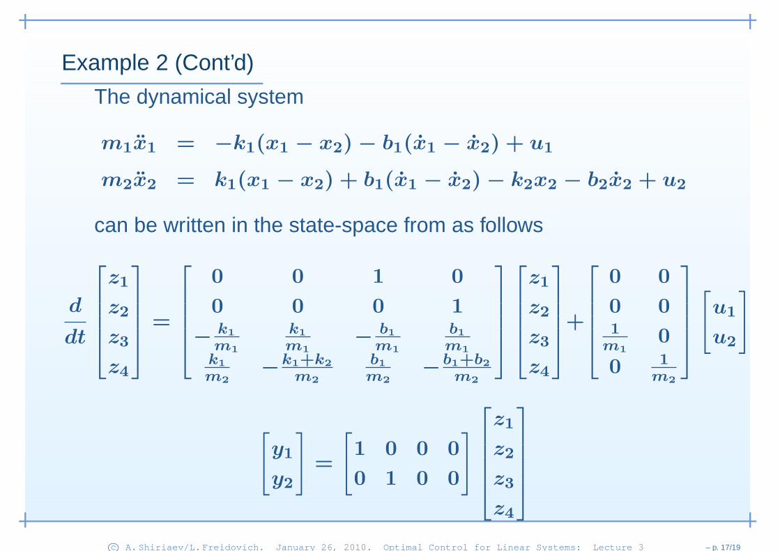
Example 2 (Cont’d)
The dynamical system
m1x1 = −k1(x1 − x2) − b1(x1 − x2) + u1
m2x2 = k1(x1 − x2) + b1(x1 − x2) − k2x2 − b2x2 + u2
can be written in the state-space from as follows
d
dt
z1
z2
z3
z4
=
0 0 1 0
0 0 0 1
− k1
m1
k1
m1
− b1
m1
b1
m1
k1
m2
−k1+k2
m2
b1
m2
−b1+b2
m2
z1
z2
z3
z4
+
0 0
0 01
m1
0
0 1m2
[
u1
u2
]
[
y1
y2
]
=
[
1 0 0 0
0 1 0 0
]
z1
z2
z3
z4
c© A.Shiriaev/L.Freidovich. January 26, 2010. Optimal Control for Linear Systems: Lecture 3 – p. 17/19
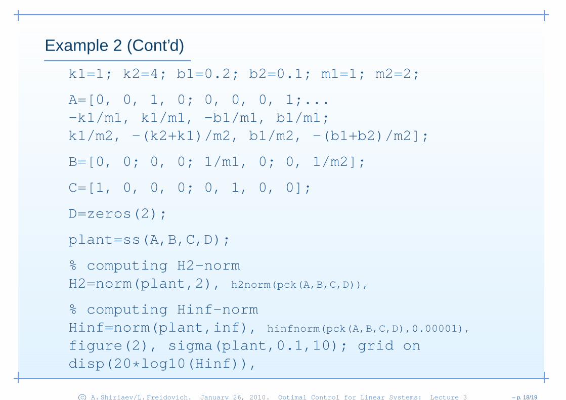
Example 2 (Cont’d)
k1=1; k2=4; b1=0.2; b2=0.1; m1=1; m2=2;
A=[0, 0, 1, 0; 0, 0, 0, 1;...-k1/m1, k1/m1, -b1/m1, b1/m1;k1/m2, -(k2+k1)/m2, b1/m2, -(b1+b2)/m2];
B=[0, 0; 0, 0; 1/m1, 0; 0, 1/m2];
C=[1, 0, 0, 0; 0, 1, 0, 0];
D=zeros(2);
plant=ss(A,B,C,D);
% computing H2-normH2=norm(plant,2), h2norm(pck(A,B,C,D)),
% computing Hinf-normHinf=norm(plant,inf), hinfnorm(pck(A,B,C,D),0.00001),
figure(2), sigma(plant,0.1,10); grid ondisp(20*log10(Hinf)),
c© A.Shiriaev/L.Freidovich. January 26, 2010. Optimal Control for Linear Systems: Lecture 3 – p. 18/19

Next Lecture / Assignments:
Next meeting: January 27, 13:15-15:00, in A205,
Next lecture (January 29, 10:15-12:00, in A206):“Well-Posedness and Internal Stability”.
c© A.Shiriaev/L.Freidovich. January 26, 2010. Optimal Control for Linear Systems: Lecture 3 – p. 19/19
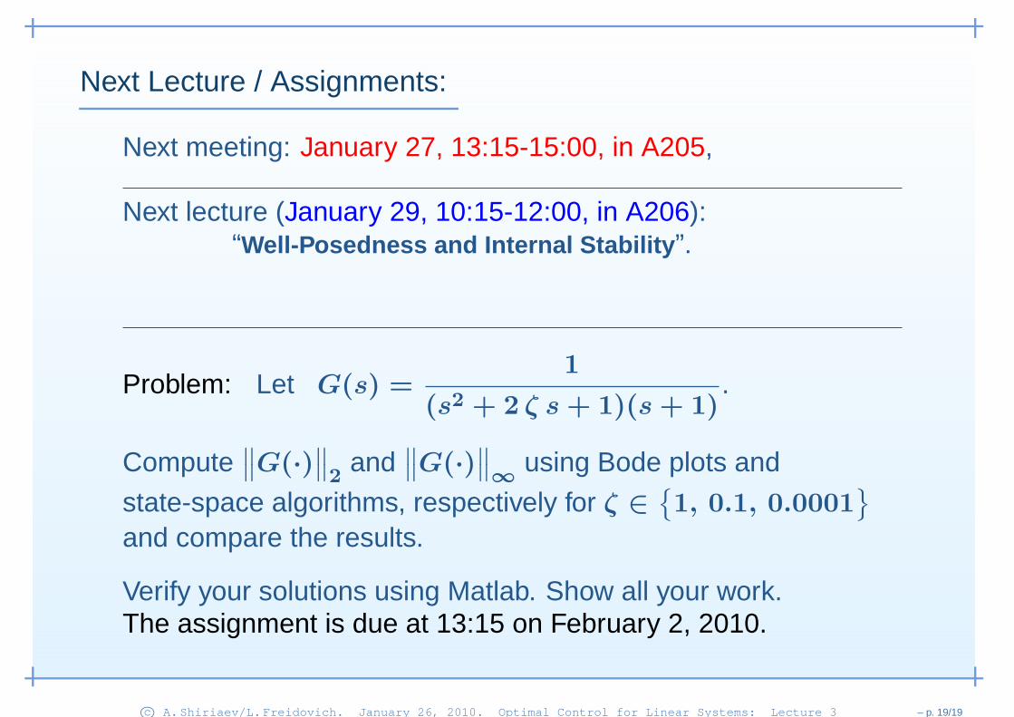
Next Lecture / Assignments:
Next meeting: January 27, 13:15-15:00, in A205,
Next lecture (January 29, 10:15-12:00, in A206):“Well-Posedness and Internal Stability”.
Problem: Let G(s) =1
(s2 + 2 ζ s + 1)(s + 1).
Compute∥∥G(·)
∥∥2
and∥∥G(·)
∥∥∞
using Bode plots and
state-space algorithms, respectively for ζ ∈{1, 0.1, 0.0001
}
and compare the results.
Verify your solutions using Matlab. Show all your work.The assignment is due at 13:15 on February 2, 2010.
c© A.Shiriaev/L.Freidovich. January 26, 2010. Optimal Control for Linear Systems: Lecture 3 – p. 19/19