toshiyasu kato and toshinao yoshiba - imes.boj.or.jp · 129 model risk and its control model risk...

129

Model Risk and Its Control


Toshiyasu Kato and Toshinao Yoshiba

Toshiyasu Kato: Corporate Risk Management Office, The Bank of Tokyo-Mitsubishi, Ltd.(E-mail: [email protected])

Toshinao Yoshida: Research Division 1, Institute for Monetary and Economic Studies,Bank of Japan (E-mail: [email protected])

This paper is the result of revisions and additions made to the original paper submitted toa research conference entitled “New Approaches to Financial Risk Management” held dur-ing January and February 2000 at the Bank of Japan. The original paper was written whilethe first author was working for the Bank of Japan. We are grateful for the numerous com-ments received from Professor Soichiro Moridaira (Keio University) and other participantsin the conference.

MONETARY AND ECONOMIC STUDIES/DECEMBER 2000

In this paper, we analyze model risks separately in pricing modelsand risk measurement models as follows. (1) In pricing models,model risk is defined as “the risk arising from the use of a modelwhich cannot accurately evaluate market prices, or which is not amainstream model in the market.” (2) In risk measurement models,model risk is defined as “the risk of not accurately estimating theprobability of future losses.” Based on these definitions, we examinevarious specific cases and numerical examples to determine thesources of model risks and to discuss possible steps to control theserisks.

Sources of model risk in pricing models include (1) use of wrongassumptions, (2) errors in estimations of parameters, (3) errorsresulting from discretization, and (4) errors in market data. On theother hand, sources of model risk in risk measurement models include(1) the difference between assumed and actual distribution, and (2)errors in the logical framework of the model.

Practical steps to control model risks from a qualitative perspec-tive include improvement of risk management systems (organization,authorization, human resources, etc.). From a quantitative perspec-tive, in the case of pricing models, we can set up a reserve to allowfor the difference in estimations using alternative models. In the caseof risk measurement models, scenario analysis can be undertaken forvarious fluctuation patterns of risk factors, or position limits can beestablished based on information obtained from scenario analysis.

Key words: Model risk; Pricing model; Risk measurement model;Risk management systems; Reserves; Scenario analy-sis; Position limits

I. Introduction

There has been an explosive growth in financial derivative products in recent years.In the case of Japan, a similar rush to develop new derivative products is expectedwith the implementation of the Financial Big Bang. Complex financial productsrequire sophisticated financial engineering capabilities for proper risk control, includ-ing accurate valuation, hedging, and risk measurement. Parallel to the creation ofmore diverse financial products and the development of new markets for such prod-ucts, both pricing models and risk measurement models used as risk managementtools have also become increasingly complex. Recently, several major financial institu-tions have reported losses arising from the use of such complex models. This hasdrawn attention to the various types of risk which result from the use of such models.

Generally speaking, the use of models can carry various types of risks.1 In thispaper, however, we specify model risks as follows. In pricing models, model risk isdefined as “the risk arising from the use of a model which cannot accurately evaluatemarket prices, or which is not a mainstream model in the market.” In risk measure-ment models, model risk is defined as “the risk of not accurately estimating the prob-ability of future losses.” Hence, such types of risk as market price input errors, andbugs remaining in software in the model-building stage are excluded from our analy-sis.

Among possible sources of model risk, there has been a great deal of discussionregarding the volatility smile (hereinafter referred to as “smile”) and the treatment ofthe distribution of underlying asset prices.2 For instance, the Black-Scholes model3

(hereinafter referred to as the “BS model”), a standard pricing model for options,assumes that underlying asset prices fluctuate according to a lognormal process,whereas actual market price fluctuations do not necessarily follow this process.

However, as pointed out by Kato and Yoshiba (1999), many market players con-tinue to use the BS model as a pricing tool with full knowledge of its limitations.Moreover, models have become indispensable tools in the development of new finan-cial products and the management of their risks. In view of this, market players nolonger have the choice of terminating the use of models on the grounds of existingmodel risks.

The purpose of this paper is to determine the sources of model risks and to dis-cuss possible steps to control their risks. The paper is organized as follows. Chapter II

130 MONETARY AND ECONOMIC STUDIES/DECEMBER 2000

1. For example, Derman (1996) refers to the following types of model risk.- Inapplicability of modelling- Incorrect model- Correct model, incorrect solution- Correct model, inappropriate use- Badly approximated solution- Software and hardware bugs- Unstable data

2. Simons (1997) states that analysis of underlying asset prices and evaluation of smile are vitally important in riskmanagement. Jorion (1999) argues that one of the causal factors in the failure of Long-Term CapitalManagement (hereinafter referred to as LTCM) was an inappropriate assumption concerning the distribution ofunderlying asset price fluctuations.

3. See Appendix 1 for details of the Black-Scholes model.

presents some cases of model risks which have actually been realized. Numericalexamples are examined in the following three chapters. Specifically, Chapter III treatslong-term foreign exchange options; Chapter IV discusses barrier options on stockprice; and Chapter V treats interest-rate strangle short strategies. Based on the impli-cations gained from these analyses, Chapter VI examines available methods for man-aging model risks. Finally, Chapter VII briefly outlines some conclusions.

II. Cases of Realized Model Risks

When are model risks realized? One such case may occur when a financial institu-tion revises its internal pricing model and registers a loss by changing its valuation ofcurrent prices. Such reports of the realization of model risks are occasionally heardfrom the market. While details of the causal factors in such cases are not made pub-lic, in this chapter, we present an outline of these cases based on media reports.4

A. Case of Index SwapIndex swaps are swap transactions in which floating interest rates are based on indicesother than LIBOR. As such, Nikkei index-linked swaps fall under this category. Inthe case of index swaps, it is necessary to manage the position and the risks in linewith the relevant index. This requires a full understanding of various types of indices,as well as the structure of index swap markets.

A certain financial institution accumulated a substantial position in a special typeof index swap. At the time, the market participants were using several types of mod-els for the valuation of this index swap. This financial institution began trading inthis product using what was recognized at the time as the leading mainstream model.As the market for this index swap shrank, some participants left the market.Thereafter, another model, which was being used by some of the remaining partici-pants, became the dominant model in the market.

While maintaining a very large position in this swap index, this financial institu-tion fell behind in research of the most dominant pricing model for this product inthe market. Consequently, it failed to recognize that a switch had been made in thedominant model until adjusting its position. As a result, it registered losses amount-ing to several billion yen when it finally adopted the new model and made the neces-sary adjustments in its current price valuations.

B. Case of Mark CapCaps5 are a form of interest rate options and generally constitute an OTC productwith relatively high liquidity. The broker screen displays the implied volatility foreach strike price and time period as calculated for cap prices using the BS model.This volatility exhibits certain skew structures (hereinafter referred to as “skew”) by

131


4. Cases cited in this section have been expressly selected for the purpose of presenting a more concrete image ofmodel risks, and may include the authorís conjectures.

5. See Kato and Yoshiba (1999) for more on interest rate cap and skew structure.

strike price and by time period. To calculate the current price of any given cap, thevolatility corresponding to the time period and strike price of the cap is first esti-mated (interpolated) on the basis of the skew which is normally observed in the mar-ket.

A certain financial institution was engaged in Deutsche mark cap transactions. Atthe time, the number of time periods and strike prices for which volatility could beconfirmed on the screen was relatively small compared to yen caps. The estimationof volatility was particularly difficult for caps with significant differences betweenmarket interest rates and strike interest rates (hereinafter referred to as “far-outstrikes”).

The financial institution was using the BS model as its internal pricing model forcaps. This institution uses the broker-screen volatility of the closest strike price as thevolatility of far-out strikes. Some cap dealers attempted to capitalize on theinevitable difference between market prices and valuation prices by trading aggres-sively in far-out strikes. This strategy generated internal valuation profits.

The financial institution fell behind in improving its pricing model and failed tominimize the gap between market prices and valuation prices. Continued cap dealertransactions under an unimproved model resulted in the accumulation of substantialinternal valuation profits. However, when the internal pricing model was finallyrevised, the financial institution reported several tens of billion yen in losses.

C. Case of Credit Spread Position Held by LTCMLTCM had accumulated a highly leveraged credit spread position which combinedemerging bonds, loans, and other instruments. The position was structured to gener-ate profits as spreads narrowed. LTCM suffered huge losses as a result of the suddenincrease in spreads following the Russian crisis in 1998.

Various reasons have been given for these huge losses. For instance, LTCM wasunable to hedge or cancel its transactions because its liquidity had dried up in themarket. On this point, it has been said that LTCM had not taken liquidity intoaccount when building its model. Others have pointed to internal problems inLTCM’s risk measurement model. Specifically, problems with wrong assumptionsconcerning the distribution of underlying asset prices and errors in data used in esti-mating the distribution of underlying asset prices have been pointed out. Bothwould lead to fatal errors in risk measurement (Jorion [1999]).

D. SummaryThe critical points in the model risks described above can be outlined as follows:- declining market liquidity and obsolescence of pricing models,- trader transactions capitalizing on the difference between market prices and prices

calculated by pricing models, and- wrong assumptions concerning the distribution of underlying asset prices and errors

in data used in estimation.The above cases indicate that very large losses can result when improvement of

internal models is neglected, or when organizational mechanisms for undertaking thenecessary improvements fail.


III. Long-Term Foreign Exchange Options

Several cases of the realization of model risks were discussed in Chapter II. InChapters III through V, model risks shall be more closely examined using numericalexamples. This exercise shall start in this chapter with the analysis of long-term for-eign exchange options.

Figure 1 presents the volatility of yen/dollar exchange rates and yen interest ratesat end-of-month as announced by the Japanese Bankers Association.

133


Figure 1 Volatility in Foreign Exchange Options (Telerate Co. as of October 29, 1999)

“Option volatility” appearing in Figure 1 presents the option volatility for timeperiods (“Term”) of less than one year, as calculated using the BS model. For thegiven day of October 29, 1999, it can be seen that the volatility structure is such thatvolatility increases as the period of the transaction is extended, going from 13.71%for a one-month transaction to 15.05% for a one-year transaction. “ATM FWD”appearing in the same figure refers to at-the-money (hereinafter referred to as“ATM”) forward transactions. This indicates the volatility of options using the for-ward foreign exchange rate of the pertinent period as the strike price.6

As shown in Figure 1, volatility for periods exceeding one year are not given. Thisis because foreign exchange options rarely exceed one year, and the transactionamount is very small even when they do. This can be explained as follows. First ofall, as compared to short-term options, long-term foreign exchange options consti-tute high-risk products because premiums become increasingly sensitive to volatilityas the maturity is prolonged. Secondly, because the market for long-term foreignexchange options is not very liquid, in certain cases a deal cannot be quickly closed.Finally, as pointed out by Derman [1996] and as can be confirmed from Figure 1,

6. In actual OTC foreign exchange option transactions, the volatility of the smile is also taken into consideration.

MONTHLY INFORMATION* OPTION VOLATILITY * *** JPY INTEREST RATE ***

ATM FWD (360 DAYS BASE)[ TERM ] [ RATE ] [ TERM ] [ RATE ] [ TERM ] [ RATE ]

1 MONTH 13.71 1 MONTH 0.04 2 YEAR 0.382 MONTH 13.96 2 MONTH 0.39 3 YEAR 0.633 MONTH 14.32 3 MONTH 0.33 4 YEAR 0.954 MONTH 14.48 4 MONTH 0.27 5 YEAR 1.285 MONTH 14.64 5 MONTH 0.26 7 YEAR 1.816 MONTH 14.81 6 MONTH 0.26 10 YEAR 2.289 MONTH 14.92 9 MONTH 0.261 YEAR 15.05 1 YEAR 0.26

[ PROVIDED BY KYODO NEWS ] [ CONTINUED ON PAGE 35303 ]

05/11 2.44 GMT [ JAPAN BANKER'S ASSOCIATION — (3) ] 35302[ OCT 29, ‘99 ]

the BS model’s assumption of constant interest rates and volatility is not realistic, par-ticularly when the term of the transaction is relatively long. As such, the valuation oflong-term foreign exchange options presents difficult problems and is especially sus-ceptible to model risks.

A. Amin-Jarrow Model7

Amin and Jarrow [1999] have developed a foreign exchange option model whichtreats two-country interest rates and foreign exchange rates as variables. Table 1 com-pares the premiums on long-term yen/dollar foreign exchange options (call options)exceeding one year (notional amount: 105.71 yen/dollar) as calculated using theAmin-Jarrow model (hereinafter referred to as the “AJ model”) and the BS model asof October 15, 1999.8 Note that the value of the correlation coefficient used in Table1 for the yen/dollar exchange rate and the dollar interest rate (0.05) was obtainedfrom historical data.

Strike prices are given in the left-hand column of Table 1, and corresponding pre-miums are indicated by option maturity. For example, for a strike price of 105.71yen/dollar (spot rate for October 15, 1999), the five-year maturity premium was 5.48yen/dollar and 5.49 yen/dollar for the AJ model and BS model, respectively. Thelargest observed difference in premiums for the two models was 0.08 yen/dollar(158.57 yen/dollar strike price with five-year maturity). This difference was equiva-lent to approximately 10% of the premiums (0.87 yen/dollar and 0.95 yen/dollar), oronly 0.076% of the notional amount. At this level, the difference can be readily con-tained in the bid-offer spread of volatility. In other words, the calculated values ofthe two models are very close to each other.


7. See Appendix 2 for details of the Amin-Jarrow model.8. Data used in the analysis consists of: yen/dollar exchange rate, and term structures of dollar and yen interest rates

of October 15, 1999; and yen/dollar exchange rate, and variance and covariance of dollar and yen interest ratesfrom October 2, 1998 to October 15, 1999 (historical data for approximately one year). In this analysis, histori-cal volatility was used. Although it is desirable to use implied volatility, historical volatility was used for the fol-lowing reasons: because of low liquidity in long-term foreign exchange option markets, it is difficult to obtainimplied volatility; and the present chapter focuses on differences in numerical results among various models.

Table 1 Comparison of Premiums (¥/$) in AJ model and BS model(Call Option for October 15, 1999)

Strike AJ model Years BS model Yearsprice 1 2 3 4 5 1 2 3 4 5

158.57 0.05 0.26 0.50 0.70 0.87 0.05 0.27 0.52 0.75 0.95148.00 0.14 0.50 0.83 1.08 1.27 0.14 0.51 0.85 1.13 1.34137.43 0.37 0.95 1.35 1.64 1.85 0.37 0.96 1.38 1.68 1.91126.86 0.95 1.75 2.20 2.48 2.67 0.96 1.76 2.22 2.52 2.71116.29 2.28 3.14 3.52 3.73 3.84 2.28 3.15 3.54 3.75 3.86105.71 4.95 5.45 5.55 5.54 5.48 4.96 5.46 5.57 5.56 5.49

95.14 9.67 9.10 8.57 8.15 7.78 9.68 9.11 8.59 8.16 7.7884.57 16.80 14.46 12.92 11.82 10.95 16.80 14.47 12.93 11.82 10.9474.00 25.95 21.70 18.84 16.80 15.23 25.95 21.71 18.86 16.82 15.2363.43 36.16 30.61 26.44 23.31 20.86 36.16 30.62 26.45 23.33 20.8652.86 46.67 40.59 35.47 31.34 27.95 46.67 40.59 35.48 31.35 27.96

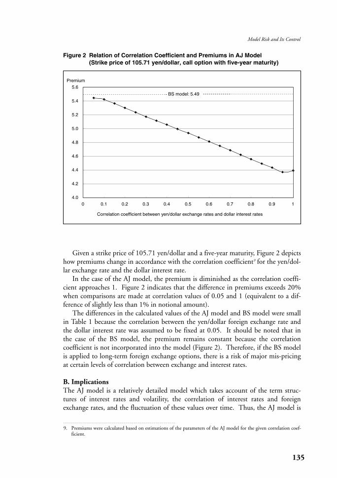
Given a strike price of 105.71 yen/dollar and a five-year maturity, Figure 2 depictshow premiums change in accordance with the correlation coefficient9 for the yen/dol-lar exchange rate and the dollar interest rate.

In the case of the AJ model, the premium is diminished as the correlation coeffi-cient approaches 1. Figure 2 indicates that the difference in premiums exceeds 20%when comparisons are made at correlation values of 0.05 and 1 (equivalent to a dif-ference of slightly less than 1% in notional amount).

The differences in the calculated values of the AJ model and BS model were smallin Table 1 because the correlation between the yen/dollar foreign exchange rate andthe dollar interest rate was assumed to be fixed at 0.05. It should be noted that inthe case of the BS model, the premium remains constant because the correlationcoefficient is not incorporated into the model (Figure 2). Therefore, if the BS modelis applied to long-term foreign exchange options, there is a risk of major mis-pricingat certain levels of correlation between exchange and interest rates.

B. ImplicationsThe AJ model is a relatively detailed model which takes account of the term struc-tures of interest rates and volatility, the correlation of interest rates and foreignexchange rates, and the fluctuation of these values over time. Thus, the AJ model is

135


9. Premiums were calculated based on estimations of the parameters of the AJ model for the given correlation coef-ficient.

Figure 2 Relation of Correlation Coefficient and Premiums in AJ Model(Strike price of 105.71 yen/dollar, call option with five-year maturity)

4.0

4.2

4.4

4.6

4.8

5.0

5.2

5.4

5.6

0 0.1 0.2 0.3 0.4 0.5 0.6 0.7 0.8 0.9 1

Correlation coefficient between yen/dollar exchange rates and dollar interest rates

Premium

BS model: 5.49

based on more realistic assumptions than the BS model. Therefore, in the valuationof long-term foreign exchange options, it is more desirable to use the AJ model thanthe BS model.

However, in the case of long-term foreign exchange options, not only is it difficultto obtain the market price, but there is no guarantee that actual transactions can becarried out at the current price calculated using the model. Moreover, there is a highrisk of mis-pricing caused by wrong estimation of the parameters.

IV. Barrier Options on Stock Price

This chapter is given to the analysis of barrier options (barrier options on stockprice), an exotic option with a complicated structure.

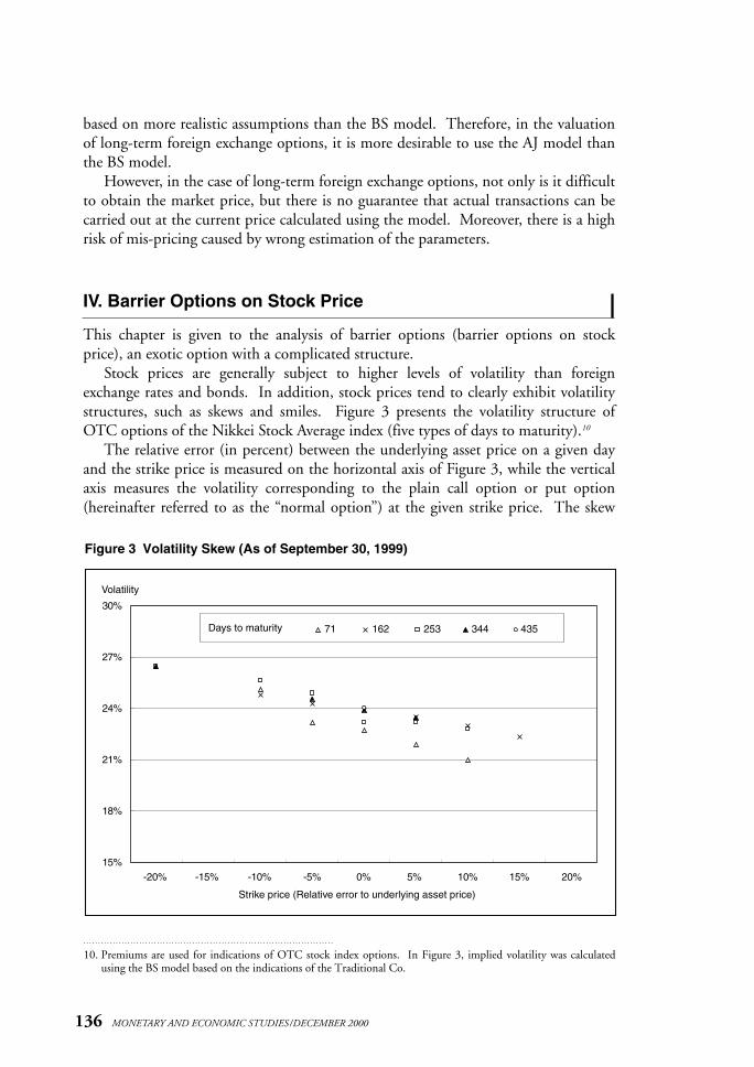
Stock prices are generally subject to higher levels of volatility than foreignexchange rates and bonds. In addition, stock prices tend to clearly exhibit volatilitystructures, such as skews and smiles. Figure 3 presents the volatility structure ofOTC options of the Nikkei Stock Average index (five types of days to maturity).10

The relative error (in percent) between the underlying asset price on a given dayand the strike price is measured on the horizontal axis of Figure 3, while the verticalaxis measures the volatility corresponding to the plain call option or put option(hereinafter referred to as the “normal option”) at the given strike price. The skew


10. Premiums are used for indications of OTC stock index options. In Figure 3, implied volatility was calculatedusing the BS model based on the indications of the Traditional Co.

Figure 3 Volatility Skew (As of September 30, 1999)

15%

18%

21%

24%

27%

30%

-20% -15% -10% -5% 0% 5% 10% 15% 20%

Strike price (Relative error to underlying asset price)

Volatility

71 162 253 344 435Days to maturity

structure of stock options is generally such that volatility is higher for options with alower strike price, and lower for options with a higher strike price. Similarly, theskew structure of options closer to maturity is more steeply sloped than options withlonger maturity. Figure 3 confirms these features of the skew structure.

To properly value the current price of stock index options and to manage the risk,it is necessary to use models which conform to market data. However, as in the caseof foreign exchange options, the BS model is widely used. This choice is based onthe fact that almost all market transactions in options constitute normal option trans-actions.

In the case of such exotic options as barrier options, it is clearly dangerous to usethe volatility of normal options for valuation of current prices and risk management.In the following section, barrier options are priced using the implied binomial treemodel (a type of lattice method), and the results are examined.

A. Implied Binomial Tree Model11

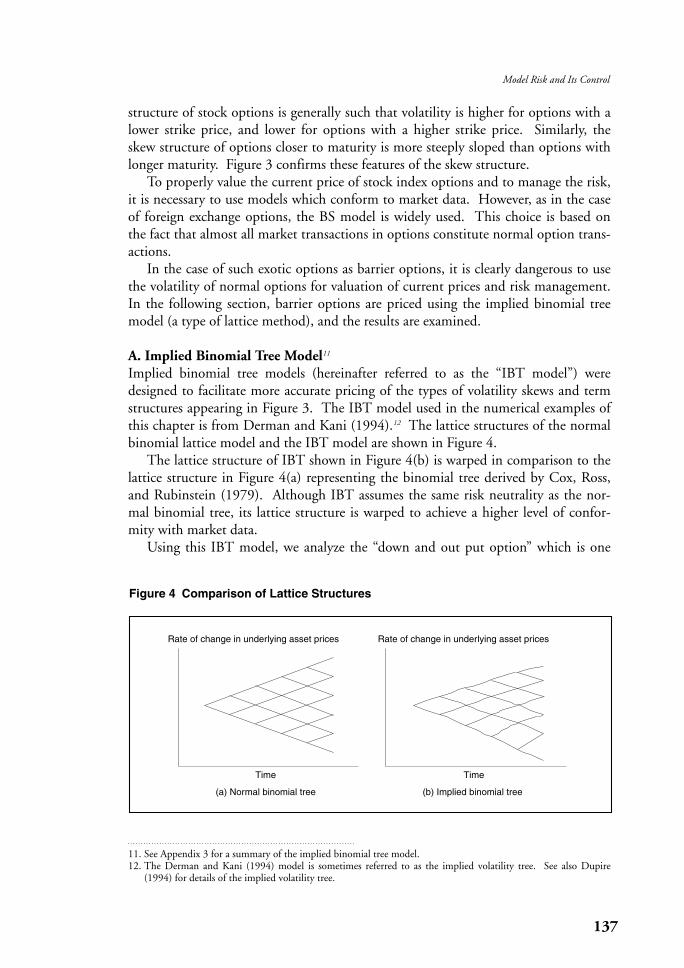
Implied binomial tree models (hereinafter referred to as the “IBT model”) weredesigned to facilitate more accurate pricing of the types of volatility skews and termstructures appearing in Figure 3. The IBT model used in the numerical examples ofthis chapter is from Derman and Kani (1994).12 The lattice structures of the normalbinomial lattice model and the IBT model are shown in Figure 4.

The lattice structure of IBT shown in Figure 4(b) is warped in comparison to thelattice structure in Figure 4(a) representing the binomial tree derived by Cox, Ross,and Rubinstein (1979). Although IBT assumes the same risk neutrality as the nor-mal binomial tree, its lattice structure is warped to achieve a higher level of confor-mity with market data.

Using this IBT model, we analyze the “down and out put option” which is one

137


11. See Appendix 3 for a summary of the implied binomial tree model.12. The Derman and Kani (1994) model is sometimes referred to as the implied volatility tree. See also Dupire

(1994) for details of the implied volatility tree.

Figure 4 Comparison of Lattice Structures

Rate of change in underlying asset prices Rate of change in underlying asset prices

Time Time

(a) Normal binomial tree (b) Implied binomial tree

type of barrier option. The down and out put option is an exotic type of optionwherein option rights are lost (the right to sell the underlying asset) if the barrierprice (hereinafter referred to as the “knock-out price”) is ever reached through matu-rity.13 The down and out put option is structured so that the rate of change in theoption price against the price of the underlying asset increases as the knock-out priceis approached.

Figure 5 compares down and out put option premiums calculated using theresults of a Black-Scholes type model (hereinafter referred to as the “BS-type”)14 andthe IBT model. The underlying asset price is 17,605.46 yen, and the knock-outprice is 15,000 yen. BS-type (strike) premiums shown in the figure were calculatedby substituting volatility at strike price into the closed-form result of the BS-type,while BS-type (knock-out) premiums were similarly calculated using the volatility ofthe knock-out price.

Figure 5 indicates that IBT model premiums15 are smaller than BS-type (knock-out) premiums, and that IBT model premiums approach the BS-type (knock-out)


13. Judgment on whether the barrier price has been reached may be based on intra-day price fluctuations, closingprices, or end-of-week prices.

14. In this paper, “BS-type analytical results” refers to calculations carried out using an option model with the sameframework as the BS model. See Appendix 1 for details.

15. All IBT model calculations in this chapter, excluding the calculations for Figure 6, are based on 30 lattice seg-ments.

Figure 5 Comparison of Down and Out Put Option Premiums (1)(As of September 30, 1999)

0

200

400

600

800

15,000 15,500 16,000 16,500 17,000 17,500 18,000

Strike price

Premium

IBTmodel BS-type (Strike) BS-type (Knock-out)

Maturity: 3 monthsKnock-out price: 15,000 yen

premiums as the strike price rises. This is an interesting observation as it means that,in comparison to the BS-type (knock-out), the IBT model assigns a greater weight tothe possibility of the underlying asset price reaching the knock-out price.

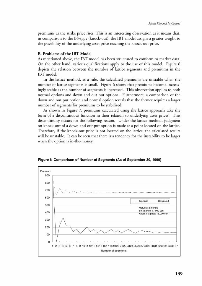
B. Problems of the IBT ModelAs mentioned above, the IBT model has been structured to conform to market data.On the other hand, various qualifications apply to the use of this model. Figure 6depicts the relation between the number of lattice segments and premiums in theIBT model.

In the lattice method, as a rule, the calculated premiums are unstable when thenumber of lattice segments is small. Figure 6 shows that premiums become increas-ingly stable as the number of segments is increased. This observation applies to bothnormal options and down and out put options. Furthermore, a comparison of thedown and out put option and normal option reveals that the former requires a largernumber of segments for premiums to be stabilized.

As shown in Figure 7, premiums calculated using the lattice approach take theform of a discontinuous function in their relation to underlying asset prices. Thisdiscontinuity occurs for the following reason. Under the lattice method, judgmenton knock-out of a down and out put option is made at a point located on the lattice.Therefore, if the knock-out price is not located on the lattice, the calculated resultswill be unstable. It can be seen that there is a tendency for the instability to be largerwhen the option is in-the-money.

139


Figure 6 Comparison of Number of Segments (As of September 30, 1999)

0

100

200

300

400

500

600

700

800

900

1 2 3 4 5 6 7 8 9 1011 1213 1415 1617 1819 20 2122 2324 2526 2728 2930 3132 3334 3536 37

Number of segments

Premium

Normal Down out

Maturity: 3 monthsStrike price: 17,000 yenKnock-out price: 15,000 yen

Figure 7 depicts the modified IBT model16 which was designed to overcome thisproblem. The modified model approximates the premium in the following manner.Two points on the lattice lying on either side of a knock-out price are assumed torepresent knock-out prices and are used in calculating two option prices located onthe lattice. Then, the difference between the closest price on the lattice and theknock-out price is linearly apportioned to approximate the premium.17 Figure 7 pre-sents a comparison of down and out put option premiums calculated using the IBTmodel and the modified IBT model.

Figure 7 shows that the premiums calculated using the modified IBT model tracea relatively smooth curve, indicating that this is an easy-to-use model from the per-spective of position management. However, compared to the BS-type (knock-out),premiums are consistently lower and move in the range of 1/2 - 2/3. This point dif-fers significantly from the results observed in Figure 5.Based on the foregoing analysis, the structures and computational processes of theIBT model and modified IBT model can be characterized as follows.

- Calculated results are more compatible to the market than the BS model.- Because these models are based on a discretized approach, the results are affected


Figure 7 Comparison of Down and Out Put Option Premiums (2)(As of September 30, 1999)

0

50

100

150

200

250

300

14,900 15,400 15,900 16,400 16,900 17,400 17,900 18,400 18,900 19,400 19,900

Underlying asset price

Premium

IBT modelModified IBT modelBS type (Knock-out)

Maturity: 3 monthsStrike price: 17,000 yenKnock-out price: 15,000 yen

16. The modified IBT model is based on the procedures of Derman, Kani, Ergener, and Bardhan (1995).17. The option price is adjusted as follows. First, the option price of a point on the lattice is calculated on the

assumption that no barrier exits at the lattice-point prices located on either side of the knock-out price. Next, thedistance (price difference) between the knock-out price and lattice-point price is linearly apportioned to theoption prices of each of the lattice points. Following this process, the option prices on the two points on the lat-tice are added together and used as the option price of the lattice point located between the two points.

141


by the discretized segments (number of segments).- An increase in the number of segments dramatically increases the computational

burden.- Reliability is low when market data is limited.- The data handling burden is high, and discretionary factors cannot be removed.

C. ImplicationsThe IBT model is designed for calculating current prices which conform to the mar-ket, based on the prices of heavily traded financial products. However, in reality, theIBT model depends on approximations such as discretization and adjustments in bar-rier prices. Therefore, the IBT model may not necessarily arrive at the theoreticallycorrect current price.

The IBT model also carries the risk of calculating a price which may not conformwith the current price at any given time. This risk arises from such considerations asthe time lag in obtaining market data, the timing of the data display output, and thebid-offer spread. Furthermore, as can be confirmed in Figure 3, a wide range of mar-ket data cannot be obtained at all times, and interpolation processes are required innumerous instances. The IBT model may be particularly susceptible to the impact ofdata interpolation.

V. Strangle Short Strategy

One of the available option strategies is a strangle short strategy. A strangle consti-tutes a combination of calls and puts with different strike prices. (A combination ofcalls and puts with the same strike price is called a straddle.) The general objectivesof making a strangle position can be described as follows. (1) Holders of options canuse strangles as a hedge against sharp swings in underlying asset prices, and (2) writ-ers of options can use strangles to earn premiums expecting that the underlying assetprice may remain within the range of the window (the range of underlying asset pricewhereby the put-call strike-price difference does not result in payment on maturity).Figure 8 presents the profit-loss diagram of the strangle short position.

Traders frequently take short positions to accommodate the hedging needs of cus-tomers.18 Moreover, some traders actively adopt a strangle short strategy featuring awide window to earn premiums. In this chapter, we shall measure the risks of strangle positions and examine somepertinent problems.

A. Interest Rate DistributionFigure 9 depicts the 10-day fluctuation histogram of a five-year swap rate. The datacovers a period of approximately six years extending between November 1993 and

18. It is more common for traders to take short positions of options in order to act as counterparties to the hedgingneeds of customers. In Japan, it appears that it is not unusual for customers to take short positions with the aimof earning premiums.

November 1999. It can be seen from Figure 9 that the distribution of interest ratefluctuations during this period differs from normal distribution which is generallyused in the value-at-risk method (hereinafter referred to as “VaR”). The center ofgravity of the actual distribution observed during this period lies to the right of nor-mal distribution (skewness = 0.28). Moreover, the historical data exhibits a kurtosisof five compared to three in the case of normal distribution. Finally, the historicaldata has a fat tail with the 99% points located at -0.41 and 0.43 (compared to 99%points located at ±0.38 in the case of normal distribution).


Figure 9 Distribution of Ten-Day Fluctuations of Five-Year Swap Rate(November 15, 1993 - November 25, 1999)

0

50

100

150

200

250

Interest rate fluctuation (10 days)

Frequency

Historical data

Normal distribution

(Average and variance werecalculated from historical data)

-0.65-0.55

-0.45-0.35

-0.25-0.15

-0.050.05

0.150.25

0.350.45

0.550.65

0.750.85

Figure 8 Strangle Short

Profit

Loss

Profit-loss line(present)

Profit-loss line(at maturity)

Underlyingasset price

B. Comparison of Risk AmountA five-year swap rate is used as the underlying asset in the following example of astrangle short strategy. Let us assume that we have sold calls and puts with strikeprices of ±0.30% from the current interest rate level. Let us further assume that thetransactions were made with ten business days remaining to maturity, and that wehold the options through maturity. Figure 10 and Table 2 present a histogram ofprofits and losses registered if one unit of the same strangle short transaction hadbeen contracted on every business day between the second half of 1996 and the firsthalf of 1999.19

Under this strangle short strategy, per unit profits amounted to 0.00 - +0.01 onnearly 90% of all trading days, indicating a very high concentration of profit/loss dis-tribution in an extremely narrow band. Cumulative profit/loss for the entire periodamounted to a gain of +0.39.20 The largest half-year gain was registered in the firsthalf of 1999 with a profit of +0.39, while the largest half-year loss was registered inthe second half of 1998 with a loss of -0.63. The largest fluctuation in profit/losswas observed during the second half of 1998. Almost all of the over ±0.05 fluctua-tions observed during the entire period were concentrated in this half-year period.Furthermore, the largest loss registered for a single transaction was also registered inthe second half of 1998 at -0.23.

Next, the relationship between profit/loss under this strangle short strategy andVaR is shown in Figure 11.

After marking a brief climb in 1994, the five-year yen-swap rate generally contin-ued to move downward until reversing itself in the second half of 1998. Thereafter,it has fluctuated in a relatively narrow band around 1%. Figure 11 shows that theprofit/loss of the strangle short strategy adopted in this chapter fluctuated signifi-cantly when the trend in interest rates was reversed. Particularly large and continu-ous fluctuations were observed during the second half of 1998. On the other hand,fluctuations were small throughout the remainder of the period.

VaR shown in Figure 11 was calculated using the scenario method and the histori-cal simulation method.21 Normal distribution was assumed for VaR (one year) andVaR (three years), and calculations were based on the worst-case scenario of the 99%(2.33 σ ) confidence level of the historical volatility for the latest one- and three-yearperiods, respectively.22 On the other hand, the 99% point of the historical simulationmethod was calculated for VaR (HS: one year) and VaR (HS: three years) based onhistorical data for the latest one- and three-year periods. Because the volatility of thefive-year swap rate continuously declined after interest rates began to climb in 1994,VaR (one year) and VaR (three years), which both assume normal distribution, traced

143


19. We assumed that we were able to sell both the call and put options based on a BS model with historical volatilityof the ten immediately preceding days with zero drift. (In reality, we could probably have received a higher pre-mium because of the existence of a smile in the market.) Note that in this chapter we are analyzing an option inwhich the five-year swap rate itself is the underlying asset.

20. Reinvestment of profits is not taken into account here.21. Standard methods for calculation of VaR of options are (1) the delta + gamma + vega method, (2) the scenario

method, and (3) the simulation method. Because (1) presents various problems for VaR measurement, (2) and(3) were used in this analysis.

22. Calculations are based on one year = 250 business days, and three years = 750 business days.


Figure 10 Profit and Loss of Interest Rate Strangle Short Strategy(Frequency distribution: October 1, 1996 - September 30, 1999)

0

20

40

60

80

100

Bel

ow-0

.14

-0.1

4

-0.1

3

-0.1

2

-0.1

1

-0.1

0

-0.0

9

-0.0

8

-0.0

7

-0.0

6

-0.0

5

-0.0

4

-0.0

3

-0.0

2

-0.0

1

0.00

0.01

0.02

0.03

0.04

0.05

0.06

0.07

Profit and loss from strangle

Frequency

888

Table 2 Profit and Loss for Interest Rate Strangle Short Strategy(Per Period: October 1, 1996 - September 30, 1999)

Data2nd 1st 2nd 1st 2nd 1st

half of half of half of half of half of half of TotalSegments

1996 1997 1997 1998 1998 1999Below -0.14 0 0 0 0 4 0 4

-0.14 0 0 0 0 1 0 1-0.13 0 0 0 0 2 0 2-0.12 0 0 0 0 0 0 0-0.11 0 0 0 0 2 1 3-0.10 0 0 0 0 0 0 0-0.09 0 1 0 0 1 0 2-0.08 0 0 0 0 1 0 1-0.07 0 0 0 0 1 0 1-0.06 0 0 0 0 0 0 0-0.05 0 0 0 1 0 0 1-0.04 0 0 0 1 0 1 2-0.03 0 0 0 0 0 0 0-0.02 0 0 0 0 1 0 1-0.01 0 0 1 1 1 0 30.00 116 121 129 121 92 109 6880.01 8 9 0 2 10 10 390.02 6 0 0 0 3 9 180.03 0 0 0 0 0 1 10.04 0 0 0 0 1 0 10.05 0 0 0 0 3 0 30.06 0 0 0 0 4 0 40.07 0 0 0 0 1 0 1

Number of Days 130 131 130 126 128 131 776Profit/Loss 0.37 0.23 0.03 -0.01 -0.63 0.39 0.39

a steady downward trend. VaR (HS: three years) also declined sharply through thefirst half of 1998 because the extreme fluctuations of 1995 were removed from thedata used for the historical simulation. Responding to market fluctuations, all VaRsbegan to climb after the second half of 1998. The most dramatic rise was observedin the case of VaR (HS: one year).

Following the reverse rise in interest rates in the second half of 1998, profit/loss ofthe strangle short strategy showed large fluctuations. Consequently, both the fre-quency and extent of excess loss over VaR were particularly high during this period(see Table 3).

Table 3 can be used to undertake the backtesting required by the market-risk reg-ulations of the Basel Committee on Banking Supervision (hereinafter referred to as“market-risk regulations”). The mandated backtesting counts the number of timesthat daily trading profit/loss has exceeded VaR (at the 99% confidence level) over thepast year. Four times or less is defined as constituting the “green zone,” five - ninetimes as the “yellow zone,” and ten or more times as the “red zone.” Financial insti-tutions whose loss frequently exceed VaR are required to add to their capital.23 Table3 indicates that the strangle short strategy of this chapter would have put us in thered zone during the second half of 1998.24

145


Figure 11 Risk Amount and Trends in Profit/Loss under Interest Rate Strangle ShortStrategy (October 1, 1996 - September 30, 1999)

0

1

2

3

Oct. 1996

Five-year swap rate(%)

-0.3

-0.2

-0.1

0

0.1

0.2

0.3VaR profit/loss

VaR(HS:3y ears)

VaR(HS:3years)

VaR(3y ears) VaR(1years)

VaR(HS:1year)

VaR(HS:1year)

VaR(1year)

Five-year swap rate

Strangle protit/loss

Strangleprofit/loss

Apr. 1997 Oct. 1997 Apr. 1998 Oct. 1998 Apr. 1999

23. Market-risk regulations require backtesting using daily profit/loss and VaR values for the latest twelve-monthperiod for each fiscal year. The backtesting results are used in determining the plus-factors to be added to themultiplication-factor of three. The plus-factor is zero for the green zone and one for the red zone. In the yellowzone, the plus-factors are 0.4, 0.5, 0.65, 0.75, and 0.85 for frequencies of excess of 5, 6, 7, 8, and 9, respectively.The market risk amount is obtained by multiplying the “multiplication-factor + plus-factor” (3 - 4) by the VaRvalue for ten business days of holding and 99% confidence level.

24. The analysis of this chapter compares profit/loss of ten business days and VaR values of ten business days of hold-ing.

C. ImplicationsIn this chapter, we have undertaken to empirically analyze risk measurement modelsand to identify pertinent problems using the strangle short strategy as a test case.Because the relation between option payoffs and underlying asset prices is non-linear,the measurement of risks is more complicated than in the case of linear payoff.

Risk measurement models are frequently based on the assumption of normal dis-tribution or lognormal distribution. Even in the case of the historical simulationmodel, it is assumed that the distribution patterns of the historical data will berepeated in the future. Because risk measurement models must contain such internalassumptions, they are inevitably susceptible to the type of model risks whereby actualdistributions differ from the assumed distribution.

VI. Practical Steps to Control Model Risks

In the foregoing chapters, we have examined model risks as separately defined forpricing models and risk measurement models. Our principal findings can be sum-marized as follows.

- Model Risks of Pricing ModelsDefinition: The risk arising from the use of a model which cannot accurately

express market prices, or which is not a mainstream model in the mar-ket.

Where market prices are obtainable, risks are realized when the valuations ofinternal pricing models are compared to actual market prices. In such cases, hedgingdiscrepancies will lead to a gradual accumulation of real profits or losses. On theother hand, where market prices are unobtainable, risks are realized when the internalpricing model is switched to the market’s dominant or mainstream model.

The sources of model risks in pricing models are generally as follows: (1) errors inthe premises and assumptions of the model; (2) errors in estimations of parameterswhich cannot be directly observed such as default probability, correlation coefficients,and other factors; (3) errors arising from discretization and other approximations;


Table 3 Frequency of Excess Loss over VaR under Interest Rate Strangle ShortStrategy (October 1, 1996 - September 30, 1999)

Risk measurement 2nd half 1st half 2nd half 1st half 2nd half 1st half Totalmethod of 1996 of 1997 of 1997 of 1998 of 1998 of 1999

VaR(3 years) Number of days exceeded 0 1 0 3 13 2 19maximum excess -0.00 -0.05 -0.23 -0.09

VaR(1 year) Number of days exceeded 0 1 0 3 12 1 17maximum excess -0.08 -0.05 -0.23 -0.03

VaR(HS:3 years) Number of days exceeded 0 0 0 3 9 1 13maximum excess -0.05 -0.23 -0.01

VaR(HS:1 year) Number of days exceeded 0 1 0 3 8 0 12maximum excess -0.08 -0.05 -0.20

and (4) errors in market data. The cases investigated in Chapter III correspond tocategories (1) and (2), while those of Chapter IV correspond to categories (3) and(4).

Probably the majority of cases of losses resulting from model risks belong to cate-gory (2), while the incidence of category (1) is thought to be quite low. Finally,model risks can be relatively easily controlled when market prices are obtainable athigh frequencies.

- Model Risks of Risk Measurement ModelsDefinition: The risk of not accurately estimating the probability of future losses.

As seen in Section II. C and Section V, one type of model risk is attributable towrong premises concerning the distribution of underlying asset prices and the failureto appropriately specify holding periods and confidence levels. In such cases, VaRcannot be accurately calculated and can lead to unexpectedly large losses. On theother hand, model risks can also take the form of over-reaction, such as unnecessar-ily large additions to the capital.

The VaR model, extensively used in the measurement of market risks, has theproblem of not being able to measure loss amounts located beyond the confidencelevel. Furthermore, in risk measurement models, logical elements of the entireframework of the model, such as computational methods and the setting of risk fac-tors for simplifying computational tasks, can also be a source of model risk.

The selection of practical steps to control model risks involves a trade-off betweenthe level of the model risk and the necessary cost of controlling the risk. Forinstance, overly rigorous examinations of models can possibly undermine the initia-tive of the model development section in developing new products. On the otherhand, if only very small positions are to be built up in a specific product, there is lit-tle justification in spending large amounts on verifying the pertinent pricing model.Furthermore, from the perspective of reducing computational burdens, a possibleapproach would be to combine the use of a relatively simple model for day-to-dayrisk control with a more refined model brought in for occasional position valuationsand the verification of the model itself. Therefore, if a necessary minimum level ofsteps has been properly installed, it could be possible to adopt a more flexibleapproach to controlling model risks while taking account of such factors as type ofproduct, transaction policy, market conditions, and size of positions.

In the following sections, we shall examine what constitutes a necessary minimumlevel of practical steps for the control of model risks.

A. Management System for Model RisksIn this section, we shall examine management systems for model risk, which may beconsidered to be necessary for financial institutions.

- Organization, Authorization, and Human ResourcesThe management of financial institutions must have a proper awareness of model

risks. Moreover, this knowledge should not be treated merely as ancillary informa-

147


tion, but must be actively utilized in management decisions. Financial institutionsmust establish independent “model control sections” which function independentlyof sections involved in the actual use of the models (such as the trading sections).Personnel in charge of model control must investigate the various models being usedby the financial institution and should be authorized to issue directives for the revi-sion and improvement of such models as needed. Finally, personnel assigned tomodel control must be able to understand the essence of the models and must befully capable of analyzing and verifying the models.

The financial institution cited in the case of the mark cap appearing in Section II.B suffered large losses, although the mark cap is a very commonplace financial prod-uct. There is a possibility that this financial institution could have averted theselosses if the personnel in its model control section had been capable of verifying themodel and had been explicitly authorized to order the implementation of necessarychanges.

- Examination of ModelsWhen a new model is developed by the trading section (hereinafter referred to as

the “front”) or the model development section, it is vitally important that it be exam-ined by an independent model examination section. The use of unexamined modelsdeveloped by the front or other sections can be extremely dangerous. As such, anexamination section which is completely independent of the front must thoroughlyexamine a new model, including such aspects as the theoretical justification (assump-tions) of the model, the conformity of prices calculated by the model and actual mar-ket prices, and hedging effectiveness. Such examination systems and protocolsshould be explicitly established in the internal rules of the financial institution.The case involving the wrong calculation of long-term foreign exchange options citedin Chapter III could have been avoided if the financial institution had instituted anappropriate model examination system. A properly manned examination sectioncould have prevented the inadvertent use of the BS model in pricing this option.

- Regular Review of ModelsThe continued use of a previously approved model without regular review can be

extremely dangerous. This is because models must regularly undergo minor adjust-ments to accurately reflect market changes, such as changes in the distribution pat-tern of underlying asset prices. Moreover, the various types of checks undertaken inthe examination process (conformity of calculated theoretical prices and actual mar-ket prices, and hedging effectiveness) must also be regularly implemented.

The implementation of regular review could have averted the very large losses suf-fered in the index swap case cited in Section II. A by calling for the necessary modifi-cations in the model at an early stage.

- Communicating with the FrontAs models are built to reflect the structure of the markets, model control staff

must have a full and up-to-date understanding of market developments. Likewise,they must be fully informed of the risk profile of the positions held by the front. It is


the front that is the closest to the market and in a position to acquire the largestamount of information concerning the market. Therefore, personnel in charge ofmodel control must maintain close and regular communications with the front, andendeavor to stay abreast of market developments and the risk profile of the currentposition.

For instance, as shown in Chapter V, positions under a strangle short strategy dis-play non-linearity (optionality), and risk measurements must take this matter intoaccount. Model control staff must have an up-to-date knowledge of the front’s cur-rent positions and position management policies, in order to develop an awareness ofpossible types of future risks and to build and manage appropriate risk measurementmodels.

B. Other Steps to Control Model RiskFurther to the model risk management systems discussed above, in this section weshall consider other types of effective steps. The specific steps examined below are:reserves against loss, scenario analysis, and position limits.

- Reserves against LossProviding reserves against loss should constitute an effective step in controlling

the model risks of pricing models.Let us consider cases in which the lattice method or Monte Carlo method is used

to calculate numerical values for pricing. When using these methods, it is not neces-sarily best to simply increase the number of segments or random number series.25 Analternative approach would be to achieve a certain level of precision in pricing whichsatisfies the requirements of the financial institution, and to thereafter depend onreserves to cope with possible calculated discrepancies. For instance, in the normalMonte Carlo method, it is known that, given N random number series, calculatederror26 will be in the order of N -1/2 . Therefore, if pricing is based on 10,000 ran-dom number series, a viable step to control model risks would be to set up a reserveequivalent to a few percent of the valuation amount.27

The use of reserves is also a viable step in cases where market data on volatilityand other factors is unobtainable. For instance, suppose that daily data on volatilityfor a particular financial product is unobtainable while monthly data is available. Inthis case, reserves can be used to cover pricing errors on all days, excluding the day onwhich volatility data is available (once a month).

Such responses would provide adequate provisions for the problems described inChapter IV, such as instability in current price resulting from too few segments underthe lattice method, or the unobtainability of volatility over a broad range.

149


25. In the computational procedures of the lattice method and the Monte Carlo method, calculated results will gen-erally approach the theoretical values as the number of segments or random number series reaches infinity. Theproblem, however, is that merely increasing the number of segments or random number series will only add tothe computational load and consume more time. Speedy pricing is particularly important in trading functions.As such, increasing the number of segments or random number series is not necessarily a viable solution.

26. See Tsuda (1995) pp. 91-113, and Kijima, Nagayama, and Omi (1996) pp. 143-155 for details of calculated dis-crepancies in the Monte Carlo method.

27. 10,000 -1/2 = 1%

- Scenario AnalysisThe front is always aware of current market conditions when using pricing mod-

els. Therefore, proper provisions must be made for dramatic market shifts whichundermine the parametric foundations of the model. One approach is to use histori-cal data (scenarios) from past incidents of dramatic market shifts to observe how theparameters of the model would have been affected in such cases, and to analyze thetrends in the discrepancies between market prices and prices calculated by pricingmodel.

One of the problems of the standard VaR model is that the model does not takeaccount of the costs of closing a position. Therefore, the question remains of how toaccount for risk when holding very large positions, or positions in low-liquidity prod-ucts. In such cases, a viable approach would be to analyze various types of scenarioswith different assumptions concerning holding period and confidence level, and dif-ferent patterns of fluctuation in risk factors.

In Chapter V, we showed that the level of VaR in the historical simulationmethod can be significantly influenced by the data observation period. Scenarioanalysis provides an effective response to such problems which are endogenous to theVaR model.

- Position LimitsOne of the available methods for reducing model risk is the setting of position

limits. For instance, position limits could be set for a product whose valuation ishighly complicated or which is subject to relatively high model risk. Such limitswould be determined in light of the corresponding level of model risk.

An example of the application of this approach to pricing models is as follows.Assume a pricing model for an infrequently traded financial product. There existsthe possibility of discrepancies arising between the internal model and other modelsused in the market. A viable response in this case would be the setting of positionlimits. This approach can be used to avoid losses arising from discrepancies betweenmarket and valuation prices, as described in Section II. A, II. B, and III. Next, in thecase of risk measurement models, information from scenario analysis can be used indetermining position limits. This approach can be used in reducing the risks whichmay result from errors in the model’s assumed distribution of underlying asset prices,as described in Section II. C and Section V.

Position limits can be managed more easily and at less cost than the process ofmodel review. Therefore, position limits can be used as a flexible and effective com-plement to the model review system.

VII. Conclusions

In this paper, we have presented various cases in which actual model risks have beenrealized and have used market data to empirically analyze the problems of the mod-els. Based on the implications of our empirical analysis, we have examined various


practical steps to control model risks. Specifically, we have used examples of index swaps, mark cap, and the experiences

of LTCM to develop a general image of model risks. From there, we have proceededto analyze long-term foreign exchange options, barrier options on stock prices, and astrangle short strategy to identify some salient features of model risk. Finally, wehave examined various steps and responses to model risks from a practical perspec-tive.

In the area of qualitative steps to control model risks, we have investigated issuespertaining to the reinforcement of risk management systems. Our investigationshave covered the following concrete issues: (1) organization, authorization, andhuman resources; (2) examination of models; (3) periodic review of models; and (4)maintenance of proper communications with the front.

In the area of quantitative steps to control model risks in pricing models, we haveproposed setting up reserves to allow for the pricing difference among different mod-els, and instituting position limits based on such differences. With regard to quanti-tative steps to control model risks in risk measurement models, we have proposedscenario analysis of various patterns in risk factor fluctuations, and instituting posi-tion limits based on the information gained from scenario analysis.

Financial institutions can, by no means, afford to ignore model risks. In thefuture, there will be a growing need to implement various types of steps to controlmodel risks, including quantitative ones.

151


APPENDIX 1: BLACK-SCHOLES TYPES

Black and Scholes (1973) assumed a lognormal distribution of stock price fluctua-tions to derive the premiums of options on stocks as the underlying asset. (BSmodel) Various other models built on the same framework as the BS model are gen-erally referred to as BS types.The option valuation formula of the BS type used in this paper is as follows.28

(Normal Option)

(A.1)

(Down and Out Put Option)

(A.2)

where: N (.) : cumulative density function of standard normal distribution,S : underlying asset price,K : strike price,H : barrier price (K > H) ,T : time to option maturity,r : risk-free domestic currency interest rate (for foreign exchange option),q : risk-free foreign currency interest rate (for foreign exchange option), σ : volatility of underlying asset price.

The price of the down and out put option can be derived by deducting the downand in put option price from the normal put option price. The option valuation for-mulas of BS-type models assume that parameters, such as interest rates and volatilityof factors other than underlying asset prices, remain constant through maturity.

Down and Out Put Normal Put Down and In Put

Down and In Put

n

= −

= − − + − + +

− − − − −

= − + = +

− − −

− −

,

( ) ( ) ( / )

[ ( ) ( )] ( / ) [ ( ) ( )],

/,

[ /( )]

Se N x Ke N x T Se H S

N y N y Ke H S N y T N y T

r qy

H SK

TT

qT rT qT

rT

1 12

12 2

1

2

2

22 1

σ

σ σ

λ σσ σ

λσ

λ

λ

,,

( / ),

( / ).x

S H

TT y

H S

TT1 1

1 1= + = +n n

σλσ

σλσ

Normal Call

Normal Put

n

n

= −= − − −

= + − +

= + − − = −

− −

− −

Se N d Ke N d

Ke N d Se N d

dS K r q T

T

dS K r q T

Td T

qT rT

rT qT

( ) ( ),

( ) ( ),

( / ) ( / ),

( / ) ( / ).

1 2

2 1

1

2

2

2

1

1 2

1 2

σσ

σσ

σ


28. See Hull (1997) pp. 457-489 for details of valuation formulas for exotic options.

APPENDIX 2: AMIN-JARROW MODEL

The BS model assumes constant interest rates and volatility through maturity.Because interest rates are less volatile than foreign exchange rates, the above assump-tion does not pose a serious problem in the case of short-term options. However,interest-rate term structures and fluctuations cannot be ignored in the case of long-term options. As such, models for long-term options must take this factor intoaccount. Amin and Jarrow (1991) developed a model which describes explicitly sto-chastic fluctuations in two-country interest rates and exchange rates. The AJ modelassumes that the forward interest rates of the two countries can be expressed inHJM29 type two-factor models, and that exchange rates can be expressed in four-fac-tor models (two factors are the same as forward interest rates models) which assumethat the rate of return follows a normal distribution. Finally, the AJ model expressesthe variance and covariance of interest and exchange rates in terms of the relationbetween the functions of the volatility of each factor.

(A.3)

Subscripts f and d are foreign and domestic interests rates for forward interestrates respectively, and:

fk (t ,T ) : forward interest rate at time T observed at time t (k : d, f ),ak (t ,T ) : forward interest rate drift (k : d, f ),σki (t ,T, fk (t ,T )) : forward interest rate volatility (k : d, f ) (two-factor),Sd (t) : foreign exchange rate,µd (t) : foreign exchange rate drift,δdi (t) : foreign exchange rate volatility (four-factor) Wi (t) : Wiener process30,

where the following relation holds.

df t T t T dt t T f t T dW t

df t T t T dt t T f t T dW t

dS t t S t dt t S t dW t

d d dii

d i

f f fi f ii

d d d di d ii

( , ) ( , ) ( , , ( , )) ( ),

( , ) ( , ) ( , , ( , )) ( ),

( ) ( ) ( ) ( ) ( ) ( ).

= +

= +

= +

=

=

∑

∑

α σ

α σ

µ δ

1

2

2

3

==∑

1

4

153


29. The Heath-Jarrow-Morton model is an interest-rate term structure model. See Heath, Jarrow, and Morton(1992) for details.

30. It is assumed that the four Wiener processes in (A.3) are mutually independent. Relations are establishedbetween the foreign exchange rate and interest rate fluctuations in the following manner. Of the four Wienerprocesses for the foreign exchange rate, two are assumed to be the same for foreign and domestic forward interestrates, and one of the Wiener processes for the foreign and domestic forward interest rates is assumed to be thesame.

Assuming that each volatility function is a deterministic function, the call optionprice can be expressed as follows.

(A.4)

Unlike the BS model, the AJ model describes explicitly term structures and fluc-tuations in the term structures of interest rates and volatility. However, in this paper,we assumed that interest rate and foreign exchange rate volatility, variance and covari-ance remained constant through maturity, and derived our calculations from histori-cal data. This choice is based on the fact that the market for long-term foreignexchange options is small and price data is difficult to obtain.

Call

1n

= − −

=+

= + −

= −

∫∑=

P T S N h KP T N h

h

P T S

KP T

a v T v a v T dv

a t T

f d d

f d

d

fi di di

T

i

ki

( , ) ( ) ( ) ( , ) ( ),

( , ) ( )

( , ),

[ ( , ) ( ) ( , )] ,

( , )

0 0 0

0 0

012

2

2 2

01

4

ζ

ζ

ζ

ζ δ

σ kikit

T

k

k kt

T

t u f t u du

P t T f t u du

∫∫= −[ ]

( , , ( , )) ,

( , ) exp ( , ) .

var( ( , ))

var( ( , ))

cov( ( , ), ( , ))

df t T t T f t T t T f t T dt

df t T t T f t T t T f t T dt

df t T df t T t T

d d d d d

f f f f f

d f d

= += +

=

[ ( , , ( , )) ( , , ( , )) ] ,

[ ( , , ( , )) ( , , ( , )) ] ,

[ ( ,

σ σσ σ

σ

12

22

22

32

2 ,, ( , )) ( , , ( , ))] ,

( )( )

( ) ,

( )( )

( , , ( , )) ( ) ,

f t T t T f t T dt

dS tS t

t dt

dS tS t

df t T f t T t dt

d f d

d

ddi

i

d

dd di d di

i

σ

δ

σ δ

2

2

1

4

1

2

var( )

cov( , (t,T))

=

=

=

=

∑

∑


APPENDIX 3: IMPLIED BINOMIAL TREE MODEL

The behavior of underlying asset prices can be expressed as follows in the type ofworld assumed in the BS model.

dS = µc Sdt + σc SdW(t). (A.5)

Here, S stands for underlying asset price, and it is assumed that drift µc andvolatility σc remain constant through maturity. W(t) is the Wiener process. Cox,Ross, and Rubinstein (1979) used a binomial tree to derive option prices, based onthe assumption that underlying asset prices exhibit this type of behavior. While itsbasic structure is the same as that of the binomial tree proposed by Cox and others,the IBT model contains the following innovative feature. Time is divided into sev-eral smaller segments, and the behavior of underlying prices within each time seg-ment is assumed to conform to the following geometric Brown movements.

dS = µ(t)Sdt + σ(S,t)SdW(t). (A.6)

The IBT model was developed to cope with interest rate term structures and othermarket phenomena, such as smiles and skews. Therefore, the functions µ(t) andσ(S,t) in (A.6) are determined to conform with option prices observed in the mar-ket. Furthermore, based on the following procedures, the normal binomial tree isdesigned to yield a regular lattice structure as shown in Figure 4(a): (1) the persteprate of increase in underlying asset prices is given as , the perstep rate ofdecline in underlying prices is given as , and the drift in underlying assetprices is given as a=eµc∆t; and (2) the upward probability is given as p=(a-d ) / (u-d ),and the downward probability is given as 1–p. On the other hand, the IBT modeluses forward induction to develop the lattice structures. In other words, when mov-ing from the starting-point asset price to the next step, the parameters µ(t) andσ(S,t), which express the stochastic processes of the underlying asset price, aredefined so that the asset price in the next step conforms to the option price observedin the market.31 For this reason, the lattice structure differs from that of the standardbinomial tree and is skewed as shown in Figure 4(b).Appendix Figure shows the distribution of underlying asset prices as deduced by theIBT model using the market data as of September 30, 1999.

As can be seen from Appendix Figure, the implied distribution of underlying assetprices derived from the IBT model does not conform with a lognormal distribution.

155


u e c t= σ ∆

d e c t= −σ ∆

31. See Derman and Kani (1994) and Rubinstein (1994) for details of structuring of lattices in the IBT model.


Appendix Figure Implied Distribution of Underlying Asset Prices in IBT model(As of September 30, 1999)

0.00

0.05

0.10

0.15

0.20

0.25

5000

7000

9000

1100

0

1300

0

1500

0

1700

0

1900

0

2100

0

2300

0

2500

0

2700

0

2900

0

3100

0

3300

0

3500

0

Underlying asset price

Probability density

Implied distribution

Lognormal distribution(derived from BS model)

157


Amin, K. I., and R. A. Jarrow, “Pricing Foreign Currency Options under Stochastic Interest Rates,”Journal of International Money and Finance, 10, 1991, pp. 310–329.

Black, F., and M. Scholes, “The Pricing of Options and Corporate Liabilities,” Journal of PoliticalEconomy, 81, 1973, pp. 637–654.

Cox, J., S. Ross, and M. Rubinstein, “Option Pricing: A Simplified Approach,” Journal of FinancialEconomics, 7, 1979, pp. 229–264.

Derman, E., “Model Risk,” Risk, 9, May, 1996, pp. 34–37.——— and I. Kani, “Riding on a Smile,” Risk, 7, February, 1994, pp. 32–39.———, ———, D. Ergener, and I. Bardhan, “Enhanced Numerical Methods for Options with

Barriers,” Financial Analysts Journal, November/December, 1995.Dupire, B., “Pricing with a Smile,” Risk, 7, January, 1994, pp. 18–20.Heath, D., R. Jarrow, and A. Morton, “Bond Pricing and the Term Structure of Interest Rates: A New

Methodology for Contingent Claim Valuation,” Econometrica, 60 (1), 1992, pp. 77–105.Hull, J., Options, Futures, and Other Derivatives, Third Edition, Prentice Hall, 1997.Jorion, P., “How Long-Term Lost Its Capital,” Risk, 12, September, 1999, pp. 31–36.Kato, Toshiyasu, and Toshinao Yoshiba, “Kin’yu Hasei Shohin Model no Jitsumuteki Katsuyo ni

Tsuite (Practical Usage of Models for Financial Derivative Products),” IMES Discussion PaperNo. 99-J-24, Institute for Monetary and Economic Studies, Bank of Japan, 1999 (in Japanese).

Kijima, Masaaki, Izumi Nagayama, and Yoshiyuki Omi, Finance Kogaku Nyumon Dai-san Bu, SuchiKeisan Ho (Introduction of Financial Engineering Part 3, Numerical Method), Nikka Giren, 1996(in Japanese).

Rubinstein, M., “Implied Binomial Trees,” The Journal of Finance, 69, 1994, pp. 771–818.Simons, K., “Model Error,” New England Economic Review, Federal Reserve Bank of Boston,

November/December, 1997, pp. 17–28.Tsuda, Takao, Monte Carlo Ho to Simulation (Monte Carlo Method and Simulation), Third Edition,

Baifukan, 1995 (in Japanese).

References

toshiyasu kato and toshinao yoshiba - imes.boj.or.jp · 129 model risk and its control model risk...

Documents