Total Quality Management

BUS 3 – 142

Statistics for VariablesWeek of Mar 14, 2011

Page 2 2

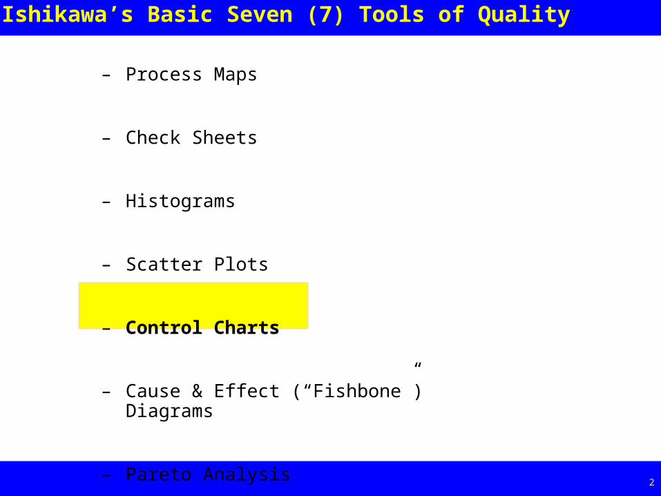
Ishikawa’s Basic Seven (7) Tools of Quality

– Process Maps

– Check Sheets

– Histograms

– Scatter Plots

– Control Charts

– Cause & Effect (“Fishbone”) Diagrams

– Pareto Analysis

Page 3 3

Reasons to carefully monitor processes

– Ensure compliance to specifications

– Continuous Improvement

– Checking for dispersion

– Look for variation and reducing the variation

– Understand Randomness vs. Abnormality

Page 4 4

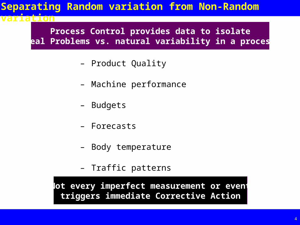
Separating Random variation from Non-Random variation

– Product Quality

– Machine performance

– Budgets

– Forecasts

– Body temperature

– Traffic patterns

Process Control provides data to isolateReal Problems vs. natural variability in a process

Not every imperfect measurement or eventtriggers immediate Corrective Action

Page 5 5

Remember

The purpose of Process Control is to quickly detect abnormal data and trends for appropriate Corrective Action and to enable Continuous Improvement

It is not about IDEAL performance, it is about Controlled, sustained performance

It is not meant to predict exact future performance but helps predict RANGES of future performance

Sampling

Page 7 7

Key Statistical Measures

Mean

– Average

Standard Deviation

– A measure of variability around the mean

– The basis for using probability in anlysis

Upper Control Limit

– A calculation around the process mean, based on a Normal Distribution

Lower Control Limit

– A calculation around the process mean, based on a Normal Distribution

Page 8 8

Monitoring Samples vs. Entire populations

– Lower cost

– Less time

– Less disruptive

– A practical alternative when destructive testing is required

Page 9 9

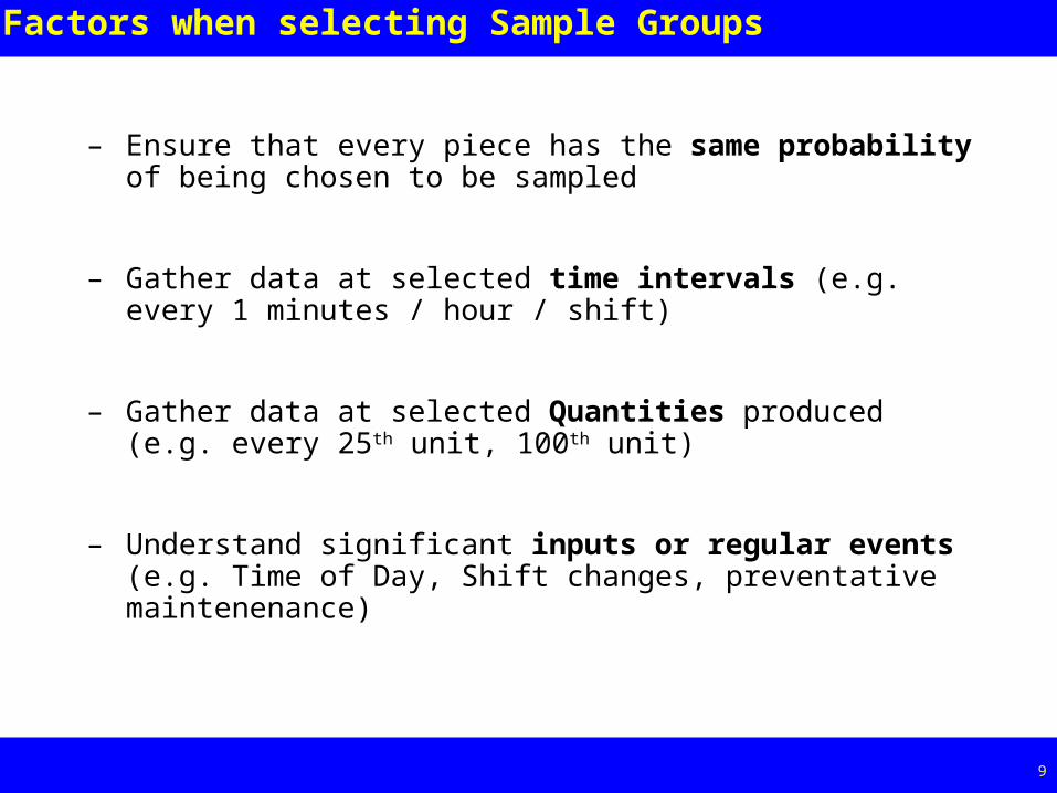
Factors when selecting Sample Groups

– Ensure that every piece has the same probability of being chosen to be sampled

– Gather data at selected time intervals (e.g. every 1 minutes / hour / shift)

– Gather data at selected Quantities produced (e.g. every 25th unit, 100th unit)

– Understand significant inputs or regular events (e.g. Time of Day, Shift changes, preventative maintenenance)

ConstructingProcess Control Charts

Page 11 11

Key Elements when implementing Process Inspection

– What Type of Inspection

– Population

– Random

– Which sub-groups

– Which critical attributes to be sampled

– Size of samples

– Who will perform the inspection

– Who will monitor and analyze the data

Page 12 12

Generalized Procedure for Developing Process Charts

1. Identify critical operations where inspection might be needed

If the operation is performed improperly, the product will be negatively affected

2. Identify critical product characteristics that will result in either good or poor functioning of the product

3. Determine whether the product characteristic is variable or attribute

4. Select the appropriate Control Chart

5. Establish the Control Limits and use the chart to continually monitor and improve

6. Update the limits when changes have been made to the process

* Adapted from Foster, Quality Management, Fourth Edition, Prentice Hall

Page 13 13

Control Charts: Variable & Attribute Data

– Variables

– Weight

– Thickness

– Height

– Heat

– Tensile strength

– Attributes

– Pass / Fail

– Defects (Parts Per Million)Variables Attributes

x (process population average) p (proportion defective)

x-bar (mean or average) np (number defective or number nonconforming)

R (range) c (number nonconforming in a consistent sample space)

MR (moving range) u (number defects per unit)

s (standard deviation)

* Adapted from Foster, Quality Management, Fourth Edition, Prentice Hall

Page 14 14

Histogram

Before using a Tool designed for a Normal Distribution,Make sure that the data are Normally Distributed

Page 15 15

Normal Distribution

Additional discussion Page 340

Page 16 16

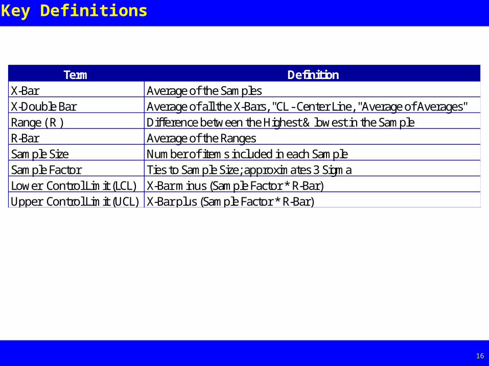
Key Definitions

Term DefinitionX-Bar Average of the SamplesX-Double Bar Average of all the X-Bars, "CL - Center Line, "Average of Averages"Range ( R ) Difference between the Highest & lowest in the SampleR-Bar Average of the RangesSample Size Number of items included in each SampleSample Factor Ties to Sample Size; approximates 3 SigmaLower Control Limit (LCL) X-Bar minus (Sample Factor * R-Bar)Upper Control Limit (UCL) X-Bar plus (Sample Factor * R-Bar)

Page 17 17

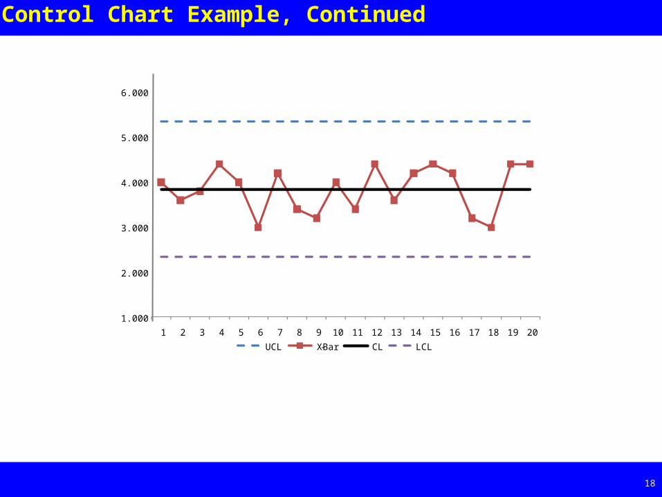
Control Chart Example

Sample 1 2 3 4 5 6 7 8 9 10 11 12 13 14 15 16 17 18 19 201 4 4 3 4 3 3 3 3 3 4 3 3 4 5 5 3 2 4 4 42 5 4 3 5 2 3 4 5 2 4 4 5 4 4 3 5 4 1 3 33 3 5 4 4 4 4 5 4 3 3 4 3 3 5 3 2 2 3 5 64 5 3 5 3 5 3 4 2 4 5 3 6 5 4 5 6 3 3 5 55 3 2 4 6 6 2 5 3 4 4 3 5 2 3 6 5 5 4 5 4

Avg (X-Bar) 4 3.6 3.8 4.4 4 3 4.2 3.4 3.2 4 3.4 4.4 3.6 4.2 4.4 4.2 3.2 3 4.4 4.4Range ( R ) 2 3 2 3 4 2 2 3 2 2 1 3 3 2 3 4 3 3 2 3

X-Double Bar (Center Line "Average of Averages") 3.84R-Bar (Average of Ranges) 2.6

Lower Control Limit (LCL) = Center Line - (Sample Factor * R-Bar)Upper Control Limit (UCL) = Center Line + (Sample Factor * R-Bar)

50.577

1 2 3 4 5 6 7 8 9 10 11 12 13 14 15 16 17 18 19 20UCL 5.340 5.340 5.340 5.340 5.340 5.340 5.340 5.340 5.340 5.340 5.340 5.340 5.340 5.340 5.340 5.340 5.340 5.340 5.340 5.340

X-Bar 4 3.6 3.8 4.4 4 3 4.2 3.4 3.2 4 3.4 4.4 3.6 4.2 4.4 4.2 3.2 3 4.4 4.4CL 3.84 3.84 3.84 3.84 3.84 3.84 3.84 3.84 3.84 3.84 3.84 3.84 3.84 3.84 3.84 3.84 3.84 3.84 3.84 3.84

LCL 2.340 2.340 2.340 2.340 2.340 2.340 2.340 2.340 2.340 2.340 2.340 2.340 2.340 2.340 2.340 2.340 2.340 2.340 2.340 2.340

Day

Out

put

Sample Factor (A2) =Sample Size =

Page 18 18

Control Chart Example, Continued

1.000

2.000

3.000

4.000

5.000

6.000

1 2 3 4 5 6 7 8 9 10 11 12 13 14 15 16 17 18 19 20

UCL X-Bar CL LCL

Page 19 19

Interpreting Control Charts

– All points lie within the Control limits

– The point grouping does not form a particular form

Control and Randomness

– Run: When points line up on the same side of the Center Line. Three points together above or below the line is a run. A run of 7 points is considered an abnormality. A run 0f 10 out of 11 or 12 out of 14 is also considered a run

– Trend: A continued rise or fall of 7 points; can cross the center line (a specific run) … Also known as “Drift”

Key signs of Non-randomness

Additional analytics on Page 345

Page 20 20

Interpreting Control Charts

Page 21 21

Additional Points on Control Charts

– Control Limits are Calculated, Specification Limits are not calculated

– The Sample Factors APPROXIMATE 3 Standard Deviations

– The smaller the sample size, the greater the uncertainty (see Factors on p347)

– Control Limits should be CONSTANT

– Recalculate UCL and LCL only after process has CHANGED

Page 22 22

Control Chart Summary

Inputs Process Outputs

•Establish Variable or Attribute Date•Define Key Characteristics to Measure•Confirm Normal Distribution•Choose Data Gathering Methodology•Train Users

•Collect Data•Plot Data•Check for Randomness

•Identify Randomness•Identify non-Randomness•Stop production if necessary•Discover improvement opportunities•Recalculate Control Limits

Page 23 23

Moving Range Charts

– Variable data only

– Volumes are very low

– Single points are recorded

– Not samples or subgroups,

– Requires a Normal distribution

Process Capability

Page 25 25

Illustration of Process Capability vs. Product Specifications

UCL

LCL

24

26

28

30

32

34

36

1 2 3 4 5 6 7 8 9 10 11 12 13 14 15 16 17 18 19 20 21 22 23 24 25

X

USL

LSL

Observation

Key

Ch

arac

teris

tic (

dim

ensi

on,

func

tion

ality

, de

liver

y, e

tc..

)

The Supplier is likely to produce conforming parts all the time

Page 26 26

Illustration of Process Capability vs. Product Specifications

UCL

LCL

24

26

28

30

32

34

36

1 2 3 4 5 6 7 8 9 10 11 12 13 14 15 16 17 18 19 20 21 22 23 24 25

X

USL

LSL

Observation

The Supplier is likely to produce a quantity of non-conforming parts

Key

Ch

arac

teris

tic (

dim

ensi

on,

func

tion

ality

, de

liver

y, e

tc..

)

Page 27 27

Applying Process Capability to Supplier Selection

– If a Supplier’s process consistently meets or exceeds Customer Specifications, consider the following:

Increasing spend on the items (if not Single Source) Introducing new items to be supplied Partnerships and collaborative design where appropriate

– If a Supplier’s process misses Customer Specifications, consider: Changing the Supplier Changing the Specification (when possible) Improving the Supplier (if business case justifies)