tourism flows model methodology

Final Report

Tourism Flows Model

Methodology

Prepared for

Ministry of Tourism

October 2006

Covec is an applied economics practice that provides rigorous and independent analysis

and advice. We have a reputation for producing high quality work that includes quantitative

analysis and strategic insight. Our consultants solve problems arising from policy, legal,

strategic, regulatory, market and environmental issues, and we provide advice to a broad

range of companies and government agencies.

Covec develops strategies, designs policy, and produces forecasts, reports, expert testimony

and training courses. Our commitment to high-quality, objective advice has provided

confidence to some of the largest industrial and governmental organisations in Australasia.

Authorship

This document was written by Shane Vuletich. For further information email

[email protected] or phone (09) 916-1961.

Disclaimer

Although every effort has been made to ensure the accuracy of the material and the integrity

of the analysis presented herein, Covec Ltd accepts no liability for any actions taken on the

basis of its contents.

© Copyright 2006 Covec Ltd. All rights reserved.

Covec Limited Level 11 Gen-i tower 66 Wyndham Street

PO Box 3224 Shortland Street Auckland New Zealand

t: (09) 916-1970 f: (09) 916-1971 w: www.covec.co.nz

Contents

1. Introduction 1

1.1. Background 1

1.2. Overview of the Tourism Flows Model 2

1.2.1. Tourism Flows Module (Dynamic Module) 2

1.2.2. Tourism Activity Module (Static Module) 4

1.3. Dimensions of the Tourism Flows Model 4

1.3.1. Report Outline 6

1.3.2. Additional Documentation 6

2. Establishing Spatial Units 7

2.1. Overall Process 7

2.2. IVS 8

2.3. DTS 11

3. Data 12

3.1. Tourism Flows Data 12

3.1.1. Seasonal Aggregations 12

3.1.2. Temporal and Geographic Aggregations 12

3.2. Static Tourism Data 22

3.3. Other Data 22

3.3.1. Transit Data 22

3.3.2. Air Route Data 22

3.3.3. Sub-Annual Trip Forecasts 23

4. Modelling 24

4.1. Data Aggregations 24

4.2. Conversion Rates 24

4.3. Forecasting Tourist Flows 25

4.4. Travel Routes 25

Appendix 27

Covec: Tourism Flows Model Methodology 1

1. Introduction

1.1. Background

The Ministry of Tourism is leading a three year project that aims to forecast the demand

tourism will place on New Zealand’s publicly provided infrastructure. The first stage of

the project investigated the mechanisms public sector agencies use to plan for growth in

demand, with a view to determining:

(a) Whether these mechanisms take tourism into account; and

(b) What information agencies need to plan for the projected growth in tourism.

This work highlighted the need for a model that takes information from the core

tourism dataset and brings it together with other relevant datasets to build a picture of

current and future tourism flows in New Zealand.

The model needs to provide public agencies with robust, easily accessible information

on future tourism demand at a sufficiently refined geographic level to make important

infrastructure-related decisions. The model would ideally contain current and future

information on transport infrastructure (road, air and other), as well as informing

decisions on the provision of tourism-related services such as water, waste, toilets,

information centres and land development administration.

Potential users of the model include, but are not limited to:

• Department of Conservation (“DOC”)

• Transit New Zealand

• Transfund

• Land Transport Safety Authority (“LTSA”)

• Local Government

• Ministry of Tourism

Understanding the impact of tourism growth on publicly-provided infrastructure will

facilitate informed decision-making on where to invest and where to adopt pro-active

policy, planning and resource allocation practices. This will ensure that future growth

in tourism results in optimum outcomes for New Zealand.

The Tourism Flows Model (TFM), funded by the Ministry of Tourism, is a software

tool developed by Covec Limited and Eagle Technology that responds to these needs.

The TFM was originally developed as an infrastructure planning tool for local

government but has since grown beyond that as an all purpose tool for understanding

tourism at the local and national levels.

Introduction


1.2. Overview of the Tourism Flows Model

The TFM has two main components:

1. The tourism flows module (dynamic module) which provides past, present and

future estimates of tourist movements in New Zealand

2. The tourism activity module (static module) which provides past, present and

future estimates of tourism activity within specific areas of New Zealand

1.2.1. Tourism Flows Module (Dynamic Module)

The TFM uses detailed data collected from tourism surveys to model the movements of

tourists around New Zealand. Each tourist implicitly makes the following decisions

prior to travelling:

1. Where do I want/need to go?

2. How will I get there?

Where do I want to go?

From a tourism flows perspective this is the most important decision of all because it is

the catalyst for all subsequent (downstream) tourism activity. The answer to this

question is usually heavily influenced by:

(a) Where you come from; and

(b) What season you are travelling in.

The data shows quite clearly that just as different nationalities have different

propensities to visit certain parts of New Zealand, New Zealanders’ travel patterns are

influenced very much by where they reside. Hence, the origins of tourists have a large

bearing on the destination(s) they choose. The other key determinant of destination is the

season – tourists have a much higher propensity to visit some areas during the

spring/summer period than they do during the autumn/winter period, and vice versa

(beaches in spring/summer and mountains in autumn/winter for example). There are

other determinants as well, most notably purpose of travel, but the data does not support

a purpose segmentation so we have concentrated on the most influential drivers of

destination choice above.

The “where do I want to go?” question is complicated significantly by the ability of

tourists to engage in multi-visit trips i.e. you may wish to go to Wellington, but could

conceivably spend time in Matamata, Taupo, and Palmerston North on the way. Hence

one trip can generate visits to multiple destinations.

The TFM is based on an origin-destination style model that models and projects the

movements of domestic and international tourists within New Zealand.

Introduction


The model uses 9 years of IVS data and 6 years of DTS data to answer the following

question:

“What percentage of people from origin X will travel between locations Y and Z using transport

mode A during period B?”

Where:

X = origin of traveller (Origin region for internationals, Regional Council for domestics)

Y and Z = 128 distinct locations/areas in New Zealand (called Tourism Flows Areas)

A = transport mode (road, air, other (not represented spatially))

B = season or annual period

Once we understand where and how people from various origins travel within New

Zealand, we combine these patterns with forecasts of visitor growth to estimate how the

demand for travel is likely to change in the future.

How will I get there?

The next decision that tourists have to make is how to get to their desired destination(s).

There are two aspects to this decision:

1. What mode of transport will I use?

2. What route will I take?

We already know the former because the origin-destination analysis (described above)

is segmented by mode of transport. We therefore need to answer to the following

question:

“Given that I wish to travel from location Y to Z using transport mode A, what route should I

take?”

Unfortunately there is nothing in the core tourism dataset that tells us which transport

corridors are used by visitors i.e. we know where they go, and what their travel

sequences are, but we don’t know which transport corridors they use to travel between

destinations.

The TFM takes the origin-destination analysis described above and overlays it with the

main air and road transport corridors to determine which corridors are most likely to be

used when travelling between destination pairs. This analysis has been conducted

using ArcView (GIS software). This modelling completes the network flow analysis by

converting travel demand to estimates of transport corridor usage.

Introduction


1.2.2. Tourism Activity Module (Static Module)

In addition to the fundamental travel decisions of where to go and how to get there, the

model also addresses the question:

“What will I do when I reach my destination?”

The key activity parameters included in the model at the RTO level are:

• Visits (by origin or purpose)

• Visitor nights (by origin or purpose)

• Expenditure (by origin or purpose)

• Accommodation type used

• Transport type used

• Activities undertaken

• Age group

• Travel style

For practical reasons the tourism activity module operates independently of the tourism

flows module.

1.3. Dimensions of the Tourism Flows Model

Tourism Flows Module (Dynamic Module)

The tourism flows module has the following dimensions.

1. Traveller types (3)

a. International traveller

b. Domestic overnight traveller

c. Domestic day traveller

2. Traveller origins (18)

a. International (8)

i. Australia

ii. Americas

iii. Japan

iv. North-East Asia

v. Rest of Asia

vi. UK/Nordic/Ireland

vii. Rest of Europe

viii. Rest of World

A concordance showing the countries that make up these regions is presented in the

Appendix.

Introduction


b. Domestic (Regional Council Areas) (10)

i. Northland

ii. Auckland

iii. Waikato

iv. Bay of Plenty

v. Gisborne/Hawke’s Bay

vi. Taranaki/Manawatu

vii. Wellington

viii. Tasman/Nelson/Marlborough/West Coast

ix. Canterbury

x. Otago/Southland

3. Year and Season (2 per year)

a. Spring/summer (combined March and December quarters of each

calendar year)

b. Autumn/winter (combined June and September quarters of each

calendar year)

4. Transport Modes (see concordances in Appendix 1) (3)

a. Road

b. Air

c. Other (not presented spatially due to the mix of transport types in this

group)

Tourism Activity Module (Static Module)

The tourism activity module has the following dimensions.

1. Area type (1)

a. Regional tourism organisation (RTO)1

2. Visitor type (2)

a. International

b. Domestic

3. Visitor Origin

a. International (8)

i. Australia

ii. Americas

iii. Japan

iv. North-East Asia

v. Rest of Asia

vi. UK/Nordic/Ireland

vii. Rest of Europe

viii. Rest of World

1 Static data is not produced at lower levels of disaggregation due to insufficient sample.

Introduction


b. Domestic (Regional Council Areas) (10)

ix. Northland

x. Auckland

xi. Waikato

xii. Bay of Plenty

xiii. Gisborne/Hawke’s Bay

xiv. Taranaki/Manawatu

xv. Wellington

xvi. Tasman/Nelson/Marlborough/West Coast

xvii. Canterbury

xviii. Otago/Southland

4. Visit year (1)

a. Annual only (1999 – 2012)

5. Measure

a. Visits

b. Nights

c. Expenditure

The visits, nights and expenditure measures can be segmented by either visitor origin or

purpose of trip (but not both at the same time).

1.3.1. Report Outline

The remainder of this document is set out as follows. Section 2 describes the process

that we have used to define the spatial layers in the model. Section 3 outlines our data

sources and how we handled the data to manage the impact of small sample sizes, and

Section 4 provides more detail on the background modelling.

1.3.2. Additional Documentation

This document describes the development of the model itself. There is a separate user

manual for the TFM which provides step-by-step instructions on how to use the model

entitled “Tourism Flows Model User Guide” which can be downloaded from

www.tourismresearch.govt.nz.


2. Establishing Spatial Units

2.1. Overall Process

The TFM is a spatial model that is designed mainly to estimate the volumes of tourists

travelling down major transport networks in New Zealand. The flow information has

been derived from the International Visitor Survey (IVS) and the Domestic Travel

Survey (DTS). These surveys capture information on the trip itineraries of international

and domestic travellers. The itinerary data allows each trip to be broken down into a

series of trip segments, with each segment starting and ending with a stop of one hour

or more in a new destination. For example, a road trip from Auckland to Wellington

and back might have resulted in a stop in Taupo of 2 hours on the way down and an

overnight stop in Palmerston North on the way back. This trip would generate the

following trip segments: Auckland – Taupo; Taupo – Wellington; Wellington –

Palmerston North; Palmerston North – Auckland. When viewed for all visitors, this

information allows us to estimate the volumes of tourists travelling directly (i.e. with no

stops of more than 1 hour) between distinct locations in New Zealand.

A major complication is that the locations in the IVS do not match the locations in the

DTS. This makes it very difficult to validly combine data from the two surveys in a

model of this nature. We therefore need to ensure that the spatial areas that we define

for the IVS are the same as the spatial areas that we define for the DTS. This is a major

exercise because there are around 185 distinct locations in the IVS and around 9,800

distinct locations in the DTS.

A further complication is that it is not practical to model flows between every possible

location in New Zealand. It is therefore necessary to define a smaller number of

locations or ‘nodes’ which are broadly representative of the main tourism origins and

destinations in New Zealand. In reality each node represents a wider tourism

catchment; hence there is just one node for each catchment. The dominant tourism

destination in each catchment is designated as the node, and the node acts as the

connection point into the various transport networks.

The catchments, henceforth referred to as tourism flows areas (TFAs), represent the

most granular spatial units in the model. A major constraint in defining the TFAs is the

need for them to aggregate easily to larger spatial units such as territorial local

authorities (TLAs) and regional tourism organisations (RTOs). It is also possible to

define TFAs so that they aggregate to regional council areas (RCAs), but the imperfect

concordance between TLAs and RCAs means that the TFAs can only be defined to

conform perfectly to one set of boundaries. Given the importance of the TFM as a local

planning tool, it was decided that the TFAs should concord perfectly with TLA

boundaries. This means that TFAs do not concord perfectly with RCAs. However, the

match is perfect for all RCAs that don’t have boundaries that cut across TLAs.

The following sections describe the method we have used to define the TFAs.

Establishing Spatial Units


2.2. IVS

Data is collected at a less refined spatial level for international visitors (185 possible

locations in the code frame) than it is for domestic visitors (circa 9,800 locations in the

code frame). It is therefore necessary to define the TFAs around the IVS locations and

then allocate each DTS location to the appropriate TFA.

When an IVS survey is conducted the respondent is asked to list all of the places he/she

visited while in New Zealand. The respondent is shown a basic map of New Zealand,

and a more detailed map if necessary, to assist with recall. If a respondent indicates a

visit to one of the 185 IVS locations then the visit is immediately coded to that IVS

location. However, if the location is not an IVS location there is no prescriptive method

of assigning that visit to an IVS location. From what we can gather one of two things

might happen: the interviewer will either code the visit to the nearest IVS location; or

the interviewer will record the non-IVS location and it will be allocated to an IVS area at

a later stage. This is problematic because it suggests that there is no consistent method

for assigning visits to non-IVS locations to IVS locations, which implies that two

separate visits to the same non-IVS location could be coded to different IVS locations.

This in turn suggests that there is no consistent set of IVS catchments underlying the

survey methodology.

We therefore had to develop IVS catchments around each of the 185 IVS locations that

reflected as accurately as possible the treatment of past visits to non-IVS locations. The

best way to do this was to observe how visits to non-IVS locations were assigned to IVS

locations post-interview (we have no way of knowing how visits to non-IVS locations

were treated during the interview). ACNielsen provided us with a list of non-IVS

locations and the IVS areas to which they were assigned post-interview.

We took this information and mapped it to get a visual summary of the spatial

relationships between the non-IVS locations and the IVS locations. We then defined

catchments around each IVS location that (a) respected these spatial relationships; and

(b) didn’t cut across any TLA or RTO boundaries. The catchments were defined mainly

as groupings of census area units, and occasionally as groupings of meshblocks in areas

with multiple IVS locations.

During this process the number of IVS catchments/locations was reduced to 128. The

reduction was due to the omission of several IVS locations which were redundant in the

code frame, and through the aggregation of locations that were in close geographic

proximity to one another and for which it was impractical and/or meaningless to

measure tourist flows between (e.g. Paihia and Waitangi).

Each of the 128 TFAs is represented by a single “node” which corresponds to the most

dominant tourism destination in that area. All tourist flows into and out of the TFA are

attributed to the node. The node connects the TFA to the main transportation networks.

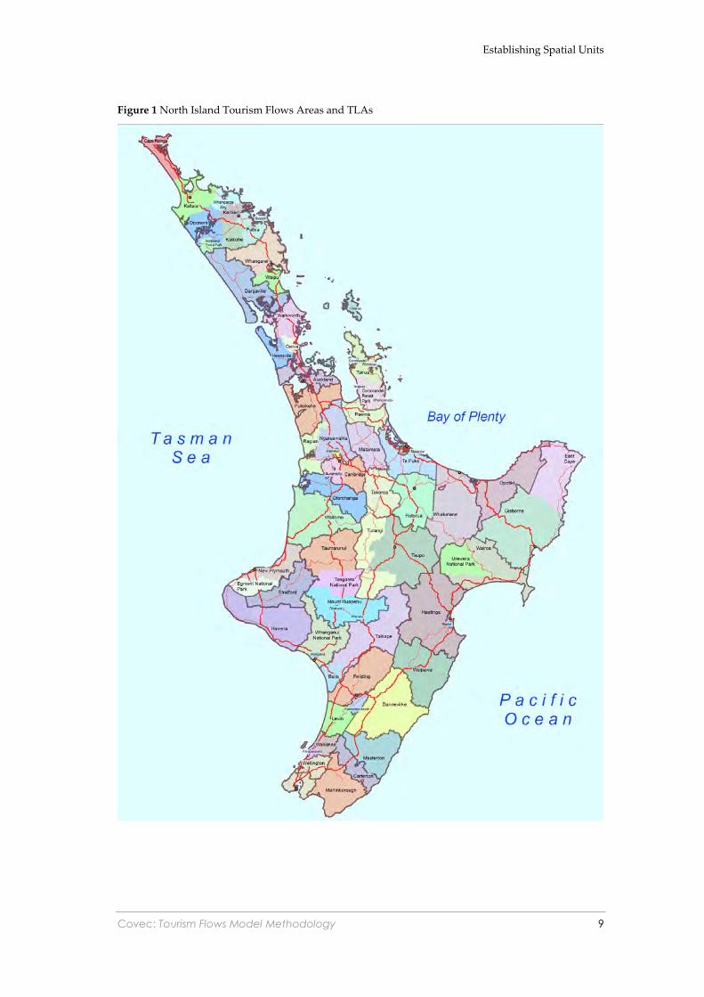
The maps below show the 128 TFAs as coloured areas, and TLA boundaries as darker

lines.



Figure 1 North Island Tourism Flows Areas and TLAs



Figure 2 South Island Tourism Flows Areas and TLAs



2.3. DTS

Once the TFAs had been defined the next step was to assign each of the approximately

9,800 DTS locations to the appropriate TFA. This was done using geocodes which

provide a northing and easting coordinate for each DTS location. The DTS locations

were mapped using these coordinates and then assigned to the TFAs that they fell

within.

A minor issue was encountered in this process when it was discovered that the original

DTS geo-codes were only accurate to within around 2km of the actual location. This

was problematic in tightly defined areas such as Arrowtown, because the DTS geocode

for Arrowtown located it in the Queenstown TFA rather than the Arrowtown TFA. It

was also problematic for DTS locations situated close to TFA boundaries because some

DTS locations were being coded to the wrong TFA.

To overcome these problems we re-geocoded as many of the DTS locations as possible,

which resulted in new and more accurate geocodes for around half of the DTS locations

in the code frame. For those locations that could not be re-geocoded we retained the

original geocodes and accepted the resulting error margin which we expect to be quite

small.


3. Data

3.1. Tourism Flows Data

The raw IVS and DTS data has been sourced from SPSS files which are held by Covec.

The data describes the number of visitor movements between each TFA node-pair,

segmented by:

• Origin of visitor (international region; regional council area)

• Type of visitor (overnight visitor; day tripper)

• Transport mode (road, air, other (not presented spatially))

• Quarter

• Year

The sample sizes are generally insufficient to provide robust estimates of tourist flows at

the finest level of segmentation. The sections below outline the methods we have used

to reduce the sample errors in the data.

3.1.1. Seasonal Aggregations

The quarterly data has been aggregated to form summer and winter seasons. The

summer season comprises the March and December quarters of each calendar year (e.g.

March 1999 and December 1999) and the winter season comprises the June and

September quarters (e.g. June 1999 and September 1999). The seasonal distinctions are

designed to pick up the differences in travel patterns between warm (beach) and cool

(mountain) periods.

3.1.2. Temporal and Geographic Aggregations

There is a clear and direct link between the accuracy of the tourism survey data and the

accuracy of the TFM. When the tourism survey data is viewed at a highly segmented

level the number of observations underlying each data point can be very small (often

only 1-2 respondents), especially for origin markets that are not heavily sampled (e.g.

the Tasman Region). The only way to overcome this problem is to aggregate the survey

data temporally and/or geographically. The tourism survey data is more reliable for

some origin markets than it is for others due to larger sample sizes. It is therefore

necessary to develop a rule that determines how the data should be aggregated for each

origin market.

The rule needs to aggregate the data as little as possible (so as not to suppress genuine

temporal and geographic variations) subject to the constraint that the resulting outputs

are statistically reliable. This requires us to define a minimum acceptable sample size

(MASS) for each market segment in the TFM, where the MASS is set at a level that

delivers statistically valid results. Any market segment that has a sample less than the

MASS will need to be aggregated further until it equals or exceeds the MASS.

Data


The rule that we have adopted requires us to:

1. Aggregate data across years within each origin x season x traveller type

combination until we have equalled or exceeded the MASS using the smallest

number of data aggregations possible; and if we cannot equal or exceed the

MASS while maintaining at least two distinct data points, then

2. Aggregate geographically similar regions until the MASS is achieved.

Method of Determining the MASS

The tourism flows modelling is based on the premise that there is some underlying

pattern or “conversion rate” between the initiation of a trip by a particular market

segment and visitations to certain locations in New Zealand. For example, it may be the

case that, on average, every 100 Australian arrivals to New Zealand generate 90 visits to

Auckland, 40 visits to Wellington and 25 visits to Queenstown. In reality we expect

these conversion rates to vary by:

• Origin market – different markets have different propensities to visit certain

locations;

• Season – for example, conversion rates for Queenstown may be a lot higher in

winter than in summer; and

• Year – for example, a lack of snow in Queenstown may have an impact on

conversion rates in a given year.

While we do expect some variation in conversion rates over time, we don’t expect a lot,

unless there are some obvious “behaviour shifters” in action during that period (such as

adverse weather conditions). This is particularly so for “mature” tourism destinations

located on main tourist routes such as Auckland, Rotorua, Taupo, Wellington,

Christchurch and Queenstown.

There needs to be some pragmatism in the final decision on MASS because each

additional aggregation of data across years reduces the number of time series data

points we have to use in the model, and each additional aggregation across geographic

regions increases the degree of homogeneity in travel behaviour. We also need to be

mindful of artificially “smoothing” out actual variations in the data by aggregating data

across either years or geographic regions.

Our analysis examines annual conversion rates with a view to testing the “stability” of

these conversion rates over time. The relative stability of the data is compared to the

underlying sample size, which provides some guidance on what the MASS should be

for the tourism flows modelling. This ultimately guides the way that we aggregate the

data for modelling purposes.

Data


Description of MASS Analysis

Our analysis is based on the premise that, on average, there is some consistent pattern

or trend to the conversation rates when viewed at the annual and seasonal levels. This

does not imply that the conversion rates are constant over time, but rather that the

conversion rates demonstrate some discernable pattern or linear time trend.

We have developed a measure of data reliability called average deviation from trend

(ADFT). The ADFT measures the deviation of the conversion rate for each origin

market in each time period and each season from the underlying linear time trend. The

underlying trend has been estimated using regression analysis.

Determining an acceptable ADFT is not easy, as the threshold will depend on the degree

of data variability that the researcher is willing to accept. In this instance we feel that a

maximum ADFT of 10% and an average ADFT of no more than 5% is acceptable for the

purposes of modelling tourism flows in New Zealand. The results of our analysis are shown

below.

International Data Aggregations

There are wide variations in sample sizes when the international data is viewed

annually, as shown in the graph below. The scatter plot shows that at the annual level

sample sizes range from around 100 to 800. It is clear from the plot that the ADFT

increases as sample size decreases, which is what we’d expect due to greater sampling

error.

Figure 3 Sample Sizes and ADFTs for Annual (Seasonal) IVS Data

0%

5%

10%

15%

20%

25%

0 100 200 300 400 500 600 700 800 900

Sample Size

Avera

ge D

evia

tion f

rom

Tre

nd

Data


For the smaller sample sizes (100-200 trips sampled) the ADFT varies quite significantly

between 5% and 20%. An ADFT of 20% indicates a high degree of variability in the

data, and we do not have confidence in the data at that level. We therefore conclude

that some of the data needs to be aggregated across time periods to achieve greater

stability.

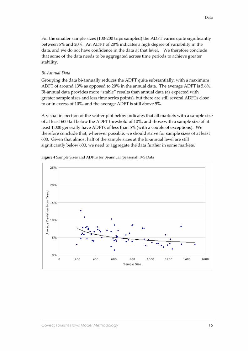
Bi-Annual Data

Grouping the data bi-annually reduces the ADFT quite substantially, with a maximum

ADFT of around 13% as opposed to 20% in the annual data. The average ADFT is 5.6%.

Bi-annual data provides more “stable” results than annual data (as expected with

greater sample sizes and less time series points), but there are still several ADFTs close

to or in excess of 10%, and the average ADFT is still above 5%.

A visual inspection of the scatter plot below indicates that all markets with a sample size

of at least 600 fall below the ADFT threshold of 10%, and those with a sample size of at

least 1,000 generally have ADFTs of less than 5% (with a couple of exceptions). We

therefore conclude that, wherever possible, we should strive for sample sizes of at least

600. Given that almost half of the sample sizes at the bi-annual level are still

significantly below 600, we need to aggregate the data further in some markets.

Figure 4 Sample Sizes and ADFTs for Bi-annual (Seasonal) IVS Data

0%

5%

10%

15%

20%

25%

0 200 400 600 800 1000 1200 1400 1600

Sample Size

Avera

ge D

evia

tion f

rom

Tre

nd

Data


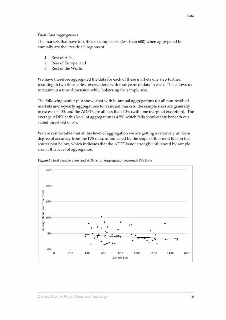
Final Data Aggregations

The markets that have insufficient sample size (less than 600) when aggregated bi-

annually are the “residual” regions of:

1. Rest of Asia;

2. Rest of Europe; and

3. Rest of the World.

We have therefore aggregated the data for each of these markets one step further,

resulting in two time series observations with four years of data in each. This allows us

to maintain a time dimension while bolstering the sample size.

The following scatter plot shows that with bi-annual aggregations for all non-residual

markets and 4-yearly aggregations for residual markets, the sample sizes are generally

in excess of 400, and the ADFTs are all less than 10% (with one marginal exception). The

average ADFT at this level of aggregation is 4.5% which falls comfortably beneath our

stated threshold of 5%.

We are comfortable that at this level of aggregation we are getting a relatively uniform

degree of accuracy from the IVS data, as indicated by the slope of the trend line on the

scatter plot below, which indicates that the ADFT is not strongly influenced by sample

size at this level of aggregation.

Figure 5 Final Sample Sizes and ADFTs for Aggregated (Seasonal) IVS Data

0%

5%

10%

15%

20%

25%

0 200 400 600 800 1000 1200 1400 1600

Sample Size

Avera

ge D

evia

tion f

rom

Tre

nd

Data


Our conclusion from this analysis is that we should aggregate the IVS data for each

market and each season as follows:

Table 1 Data Aggregations for IVS Data

Market (RLPR) Data Aggregation

Australia 2 year increments

Americas 2 year increments

Japan 2 year increments

North-East Asia 2 year increments

Rest of Asia 4 year increments

UK/Nordic/Ireland 2 year increments

Rest of Europe 4 year increments

Rest of the World 4 year increments

The data has been aggregated according to these increments on a rolling basis e.g. in the

case of a two year increment the 2004 estimates would be generated from 2003 and 2004

data, and the 2005 estimate would be generated from 2004 and 2005 data.2

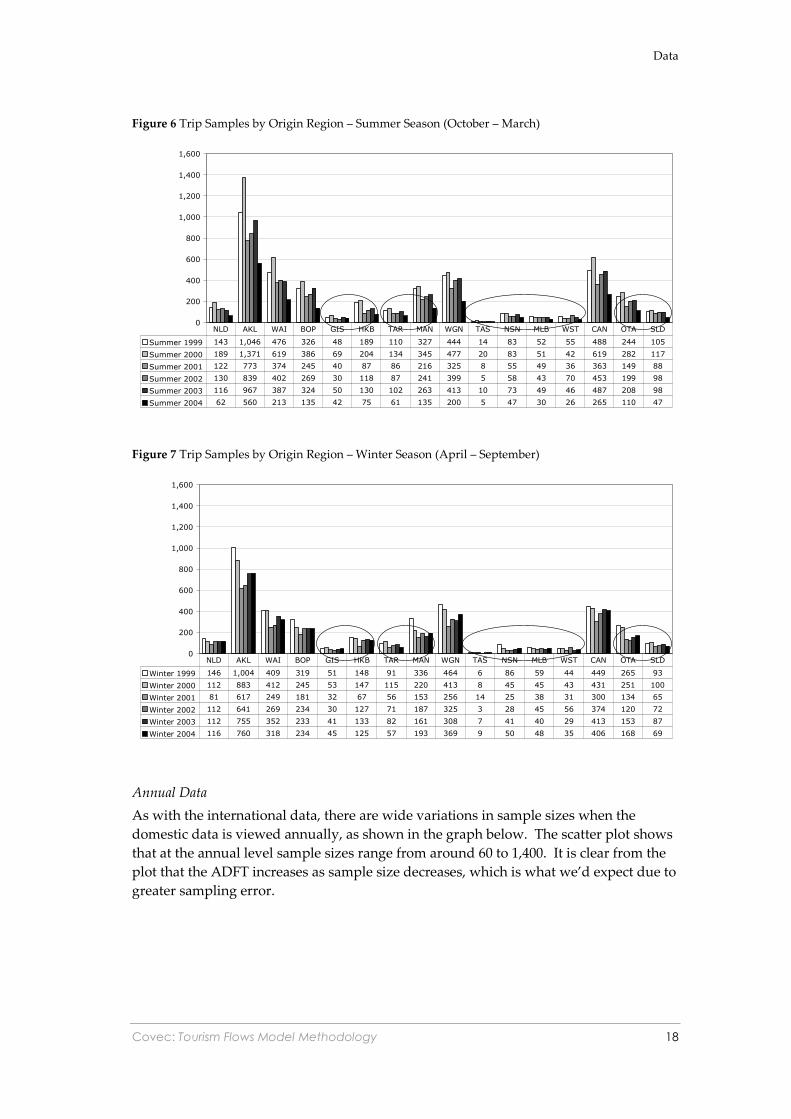
Domestic Data Aggregations

A close inspection of the DTS data reveals a relatively small number of trips sampled

out of the origin regions of Northland, Hawke’s Bay and Taranaki, and a very small

number of trips out of Gisborne, Tasman, Nelson, Marlborough, the West Coast and

Southland. To conduct a meaningful ADFT analysis we need to aggregate some of the

origin regions prior to aggregating across time periods. The necessary aggregations are:

1. Gisborne + Hawke’s Bay

2. Taranaki + Manawatu

3. Tasman + Nelson + Marlborough + West Coast

4. Otago + Southland

The Northland sample is also quite low, but we have chosen to express it as a separate

origin region rather than combining it with the major source market of Auckland. The

geographic aggregations are consistent across seasons and are shown in the graphs

below.

2 Professor Pip Forer of the University of Auckland initially suggested the rolling method.

Data


Figure 6 Trip Samples by Origin Region – Summer Season (October – March)

0

200

400

600

800

1,000

1,200

1,400

1,600

Summer 1999 143 1,046 476 326 48 189 110 327 444 14 83 52 55 488 244 105

Summer 2000 189 1,371 619 386 69 204 134 345 477 20 83 51 42 619 282 117

Summer 2001 122 773 374 245 40 87 86 216 325 8 55 49 36 363 149 88

Summer 2002 130 839 402 269 30 118 87 241 399 5 58 43 70 453 199 98

Summer 2003 116 967 387 324 50 130 102 263 413 10 73 49 46 487 208 98

Summer 2004 62 560 213 135 42 75 61 135 200 5 47 30 26 265 110 47

NLD AKL WAI BOP GIS HKB TAR MAN WGN TAS NSN MLB WST CAN OTA SLD

Figure 7 Trip Samples by Origin Region – Winter Season (April – September)

0

200

400

600

800

1,000

1,200

1,400

1,600

Winter 1999 146 1,004 409 319 51 148 91 336 464 6 86 59 44 449 265 93

Winter 2000 112 883 412 245 53 147 115 220 413 8 45 45 43 431 251 100

Winter 2001 81 617 249 181 32 67 56 153 256 14 25 38 31 300 134 65

Winter 2002 112 641 269 234 30 127 71 187 325 3 28 45 56 374 120 72

Winter 2003 112 755 352 233 41 133 82 161 308 7 41 40 29 413 153 87

Winter 2004 116 760 318 234 45 125 57 193 369 9 50 48 35 406 168 69

NLD AKL WAI BOP GIS HKB TAR MAN WGN TAS NSN MLB WST CAN OTA SLD

Annual Data

As with the international data, there are wide variations in sample sizes when the

domestic data is viewed annually, as shown in the graph below. The scatter plot shows

that at the annual level sample sizes range from around 60 to 1,400. It is clear from the

plot that the ADFT increases as sample size decreases, which is what we’d expect due to

greater sampling error.

Data


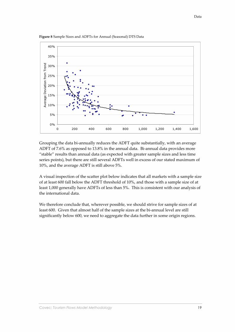
Figure 8 Sample Sizes and ADFTs for Annual (Seasonal) DTS Data

0%

5%

10%

15%

20%

25%

30%

35%

40%

0 200 400 600 800 1,000 1,200 1,400 1,600

Avera

ge D

evia

tion fro

m T

rend

Grouping the data bi-annually reduces the ADFT quite substantially, with an average

ADFT of 7.6% as opposed to 13.8% in the annual data. Bi-annual data provides more

“stable” results than annual data (as expected with greater sample sizes and less time

series points), but there are still several ADFTs well in excess of our stated maximum of

10%, and the average ADFT is still above 5%.

A visual inspection of the scatter plot below indicates that all markets with a sample size

of at least 600 fall below the ADFT threshold of 10%, and those with a sample size of at

least 1,000 generally have ADFTs of less than 5%. This is consistent with our analysis of

the international data.

We therefore conclude that, wherever possible, we should strive for sample sizes of at

least 600. Given that almost half of the sample sizes at the bi-annual level are still

significantly below 600, we need to aggregate the data further in some origin regions.

Data


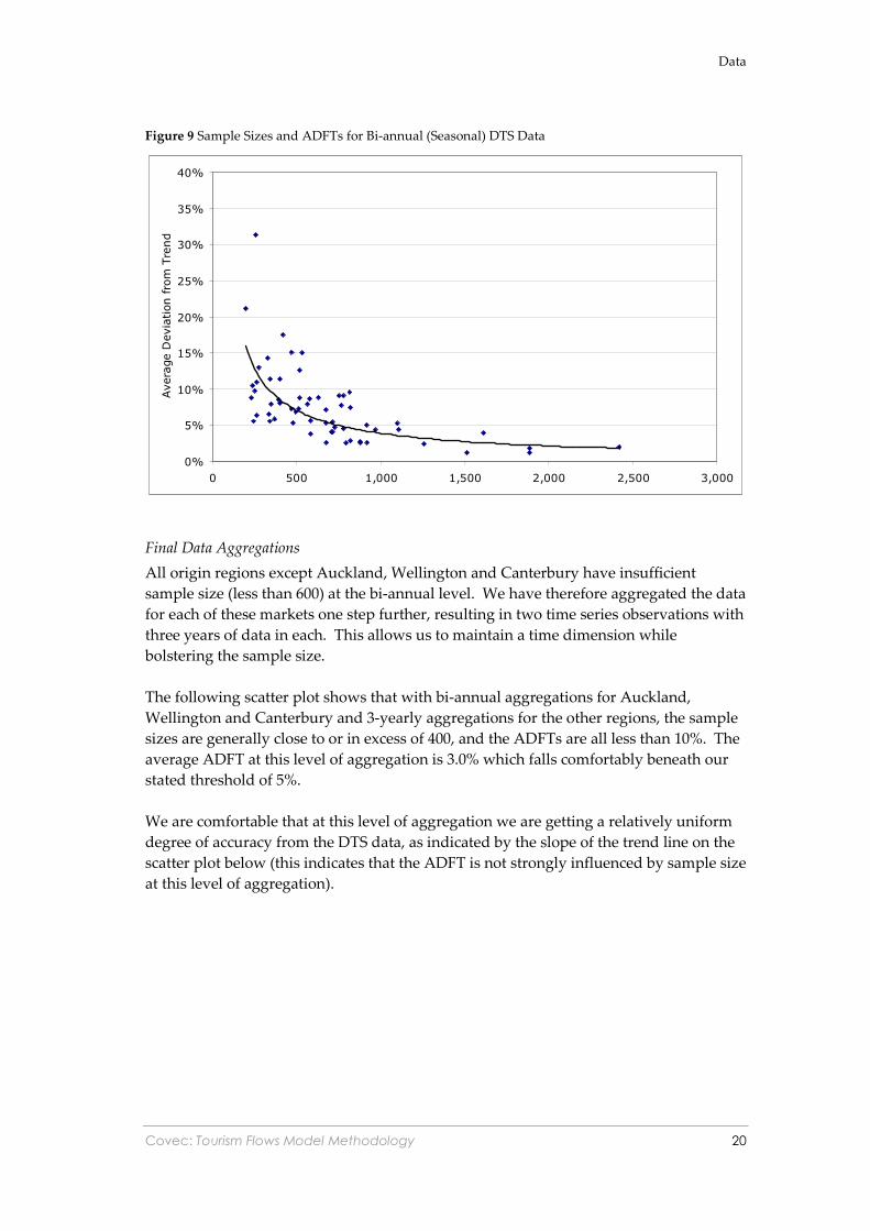
Figure 9 Sample Sizes and ADFTs for Bi-annual (Seasonal) DTS Data

0%

5%

10%

15%

20%

25%

30%

35%

40%

0 500 1,000 1,500 2,000 2,500 3,000

Avera

ge D

evia

tion fro

m T

rend

Final Data Aggregations

All origin regions except Auckland, Wellington and Canterbury have insufficient

sample size (less than 600) at the bi-annual level. We have therefore aggregated the data

for each of these markets one step further, resulting in two time series observations with

three years of data in each. This allows us to maintain a time dimension while

bolstering the sample size.

The following scatter plot shows that with bi-annual aggregations for Auckland,

Wellington and Canterbury and 3-yearly aggregations for the other regions, the sample

sizes are generally close to or in excess of 400, and the ADFTs are all less than 10%. The

average ADFT at this level of aggregation is 3.0% which falls comfortably beneath our

stated threshold of 5%.

We are comfortable that at this level of aggregation we are getting a relatively uniform

degree of accuracy from the DTS data, as indicated by the slope of the trend line on the

scatter plot below (this indicates that the ADFT is not strongly influenced by sample size

at this level of aggregation).

Data


Figure 10 Final Sample Sizes and ADFTs for Aggregated (Seasonal) DTS Data

0%

5%

10%

15%

20%

25%

30%

35%

40%

0 500 1,000 1,500 2,000 2,500 3,000

Avera

ge D

evia

tion fro

m T

rend

Our conclusion from this analysis is that we should aggregate the DTS data for each

region and each season on a rolling basis as follows,:

Table 2 Data Aggregations for DTS Data

Market (RLPR) Data Aggregation

Northland 3 year increments

Auckland 2 year increments

Waikato 3 year increments

Bay of Plenty 3 year increments

Gisborne/Hawke’s Bay 3 year increments

Taranaki/Manawatu 3 year increments

Wellington 2 year increments

Tasman/Nelson/Marlborough/West Coast 3 year increments

Canterbury 2 year increments

Otago/Southland 3 year increments

General Findings

In general both the IVS and DTS data showed a high degree of stability when the

number of trips sampled from an origin market (international) or region (domestic)

were in excess of 600. This has important implications for IVS and DTS surveying – trip

sample quotas should be set for each origin market/region so that the data is more

uniformly reliable across the country.

Data


3.2. Static Tourism Data

The static tourism data has been taken mainly from the Ministry of Tourism’s

forecasting programme, with supplementary data sourced from other data held by the

Ministry of Tourism. The regional component of the forecasting programme was

reviewed and altered in 2005 to ensure that the outputs met the needs of the TFM. The

base visits and nights data for the forecasting programme was sourced annually at the

RTO level, segmented by origin of traveller and purpose of visit. The resulting visits,

nights and expenditure forecasts were then used as inputs to the TFM.

The travel style, age, activity, transport type and accommodation data have all been

sourced from the IVS and DTS.

3.3. Other Data

3.3.1. Transit Data

Transit New Zealand has provided us with data from its continuously monitored

telemetry sites on state highways. We have sourced this data at an annual average daily

level for each month and have converted these figures to seasonal totals (spring/summer

and autumn/winter). The seasonal totals have been used to estimate the total traffic

flow at the telemetry site location in each season, expressed in terms of vehicle

movements. The vehicle movement data has been converted to estimates of passenger

movements by multiplying total vehicle movements by the average number of

occupants per vehicle. The average number of occupants per vehicle across all vehicle

types has been estimated at 4.53. The estimated tourist flows are divided by the

estimates of total passenger movements from the vehicle count data to determine the

percentage of total passenger traffic that is generated by tourists in the selected time

period.

3.3.2. Air Route Data

The tourism data provides detailed information on the trip segments that tourists

generate. However, the data doesn’t say anything about the specific route they took. In

most cases there is only one feasible route between two locations, but in some cases

there are two or more possible routes.

3 This has been based on the ratio of passenger-km by cars and campervans (8,430 million pkm, both

domestic and international) compared with coaches/buses (949 million pkm), and assumed occupancy

rates of 2 passengers per light vehicle and 25 per heavy vehicle (see Becken, S. (2002). Tourism and

Transport in New Zealand – Implications for Energy use. TRREC Report No. 54, July 2002; Becken, S. &

Cavanagh, J. (2003). Energy efficiency trend analysis of the tourism sector. Research Contract Report:

LC02/03/293. Prepared for the Energy Efficiency and Conservation Authority).

Data


In the case of air travel there is often an indirect alternative to the direct route requiring

one or more stopovers. To estimate the number of passenger movements down a

particular air segment we required information on how people travel between

destinations. For example, suppose 80% of the 100,000 passengers flying from

Auckland to Christchurch fly direct while the remaining 20% fly via Wellington. The

passengers flying from Auckland to Christchurch would therefore generate 80,000

passenger movements on the AKL-CHC segment (the direct movements) and 20,000

passenger movements on both the AKL-WGN and WGN-CHC segments (the indirect

movements).

Air New Zealand was able to provide us with the information we required to route

passengers down air segments in New Zealand based on their origin and final

destination. In cases where Air New Zealand was not the only carrier they provided

estimates of competitor behaviour. This allowed us to flow passengers through the

New Zealand air route network as accurately as possible.

3.3.3. Sub-Annual Trip Forecasts

International

The Ministry of Tourism’s forecasting programme generates monthly forecasts of

international arrivals (trips) by origin region over a 2 year horizon. We used the same

methodology to extend the forecasts a further 5 years to 2012, and have aggregated

these forecasts to form seasonal totals.

Domestic

The Ministry of Tourism’s forecasting programme generates annual forecasts of

domestic day and overnight trips out to 2012. There is no reliable data collected in the

DTS to indicate monthly demand patterns so we used monthly data from the

Commercial Accommodation Monitor (CAM) to establish this pattern. The CAM

collects monthly data by origin of traveller for most RTOs in New Zealand, and every 3

months for the rest. A notable omission in the monthly data is Auckland which

captures around 15% of all domestic visitor nights in New Zealand.

We sourced data by origin of traveller for all RTOs that collected monthly data and

aggregated this data across RTOs to derive a national estimate of monthly travel

patterns. These patterns were very consistent across both RTOs and time which gave us

a high level of confidence in the suggested monthly travel patterns. We used this data

to form a seasonal distribution in percentage terms and applied these percentages to the

annual estimates of domestic trips by origin from the Ministry of Tourism’s forecasting

programme.


4. Modelling

4.1. Data Aggregations

The data aggregations detailed in the previous section require a considerable amount of

modelling. The first level of aggregation is from quarters to seasons. This is relatively

straightforward as it is simply a case of collapsing the March and December quarters of

each calendar year into the spring/summer season and the June and September quarters

into the autumn/winter season. It is assumed that the seasonal travel patterns (as

distinct from the travel volumes) are the same as the travel patterns in the quarters that

make up the season.

The next level of aggregation is years. If an origin market is deemed to have insufficient

sample in a given year then seasons are aggregated across subsequent years until the

minimum acceptable sample size is reached. In this case data for the optimal number of

seasons is added together across years and treated as being representative of the whole

period for which data has been aggregated. The resulting annual conversion rates

(discussed in the next section) will therefore be constant for a given origin market across

the entire aggregated time period.

The final level of aggregation is geographic. If an origin market is deemed to have

insufficient sample even after data has been aggregated across years then adjacent

geographic regions are aggregated until the minimum acceptable sample size is reached.

The resulting annual conversion rates will therefore be constant for all of the markets in

the geographic aggregation within each aggregated time period.

4.2. Conversion Rates

The model uses conversion rates to translate trip numbers to estimates of passenger

movements along trip segments. The conversion rate is influenced by the attributes of

the trip such as what type of trip it is, who is taking it, what season they’re taking it in

and in which year.

Conversion rates are derived from the historical data by dividing the number of

observed trip segment flows by the total number of trips. This calculation is done for

every origin market x trip segment x time period x season x travel mode x travel type

combination. The conversion rates derived from aggregated data are assumed to apply

to every season, year and geographic region within the aggregation. The trip number

data has been aggregated in exactly the same way as the trip segment data to ensure

that the resulting conversion rates are valid.

The historical flows are derived by multiplying the appropriate conversion rates by the

trips generated in the selected time period. For example, if the user wants to observe

tourism flows for the season of autumn/winter 2003 the model calls the conversion rates

for autumn/winter 2003 and multiplies them by the trips taken in autumn/winter 2003.

If the user wants to observe tourism flows for the year of 2003 the model calls the

Modelling


conversion rates for each season in 2003 and cross multiplies these with the trips taken

in each season of 2003 and sums them to get an annual total.

4.3. Forecasting Tourist Flows

The process used to forecast tourist flows is the same as that used to estimate historical

flows – projected seasonal conversion rates are multiplied by projected seasonal trip

numbers and aggregated to fit the selected time period. The forecasts of trip numbers

are an extension of the Ministry of Tourism’s forecasting programme and are readily

available. However, it is more difficult to develop forecasts of conversion rates because:

1. There are a large number of them when all possible data segmentations are

taken into account;

2. Changes in market research providers and survey methodologies have

generated steps or trends in the data that may not be real. An example of this is

the more stringent enforcement of the 80km round-trip threshold for day trips

from 2003 onwards which significantly reduced the number of day trips

observed from that point forward. Any forecast of this data would project

forward a strong downward trend. However, in reality we know that this trend

has been generated by a change in methodology and not a real shift in the data,

so any forecasts generated from the historical data would be misleading.

Given that there have been provider changes and methodology changes in both the IVS

and DTS we felt that the best way to forecast the conversion rates was to assume that

they remain unchanged at the most recent observed value over the forecast period. We

therefore assume that the travel patterns of each market segment remain unchanged over

time relative to current values. This does not mean that aggregate travel patterns will

remain unchanged over time, because market segments are expected to grow at

different rates. Changes in travel patterns are therefore driven by changes in market

composition over time and not by changes in travel patterns within market segments.

4.4. Travel Routes

The final step in the process is to assign the identified tourist flows between each

location pair to specific transport routes. A prerequisite for routing is a comprehensive

transport network for tourists to flow through. The road network includes all state

highways as well as roads that are likely to be attractive to tourists (e.g. established

tourist routes).4 The air network includes all sectors served by Air New Zealand and

Qantas as well as tourist sectors served by other airlines. The ‘other’ transport category

captures all non-road/air modes of transport and does not have a specific network to

flow tourists though; hence these flows have not been represented spatially in the

model.

4 There are still some gaps in the modeled transportation network which the Ministry of Tourism

intends to fill over time.

Modelling


The routing procedure starts with the estimated number of passenger flows between

each location pair. In theory there are over 16,000 possible location pairs in the flows

model (128 x 128), although in practice many of these location pairs have no direct flows

recorded against them (e.g. Cape Reinga to Dunedin).

The next step is to take each location pair and decide which route(s) tourists will take to

travel between the two points. In some cases there is only one possible route between

two locations, and in other cases there are multiple routes. In the case of multiple routes

there is often only one viable route, while in the remainder of cases there will be more

than one viable route. In general the number of possible routes will increase with the

length of the trip segment (all other things being equal). The choice of route will

ultimately depend on the preferences of the traveller - some will opt for the fastest route

while others will opt for longer scenic routes.

Unfortunately little is known about the road route behaviour of tourists in New

Zealand. In the absence of better information we have developed an algorithm in

ArcView that assigns road passenger flows to specific routes based initially on travel

time (as estimated by ArcView based on factors such as distance, straightness of road

etc) and ‘tourist value’ (represented by the attractiveness of popular tourist routes).

We acknowledge that this process is reasonably “blunt” when compared with the rest of

the model. However, we still expect the road routing to be quite accurate because many

of the trip segments are quite short and therefore only have one viable route. The

majority of the error will therefore be associated with the routing of long trip segments.

The routing of air segments is much more accurate and has been based on detailed route

information provided by Air New Zealand.


Appendix

Table 3 Concordance for IVS Transport Modes

IVS Transport Category Final Transport Mode

Backpacker Bus

Campervan

Coach Tour/Tour Coach

Company Car/Van

Motorbike

Private Campervan/Motorhome/RV

Private Car/Van

Rental Campervan/Motorhome/RV

Rental Car/Van

Scheduled Coach Service

Taxi/Limousine/Car Tour

Airline

Helicopter

Private Aeroplane

Bicycle

Don't Know

Hitchhiking

Other

Refused

Train

Walking/Tramping

Cruise Ship

Interisland Ferry

Other Commercial Ferry/Boat

Private Yacht/Boat

Air

Other

Road

Appendix


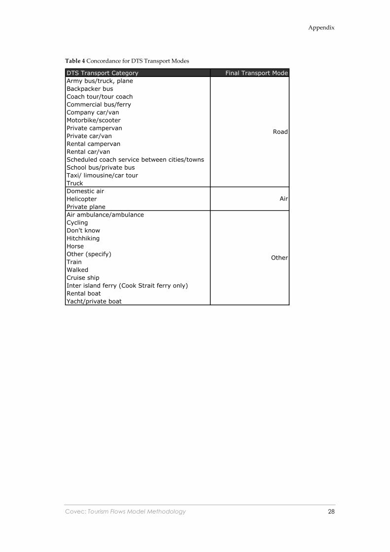
Table 4 Concordance for DTS Transport Modes

DTS Transport Category Final Transport Mode

Army bus/truck, plane

Backpacker bus

Coach tour/tour coach

Commercial bus/ferry

Company car/van

Motorbike/scooter

Private campervan

Private car/van

Rental campervan

Rental car/van

Scheduled coach service between cities/towns

School bus/private bus

Taxi/ limousine/car tour

Truck

Domestic air

Helicopter

Private plane

Air ambulance/ambulance

Cycling

Don't know

Hitchhiking

Horse

Other (specify)

Train

Walked

Cruise ship

Inter island ferry (Cook Strait ferry only)

Rental boat

Yacht/private boat

Air

Other

Road

Appendix


Table 5 Concordance for Countries and International Regions

Region of Last Permanent

Residence (RLPR)

Country of Last Permanent

Residence (CLPR)

Australia Australia

Americas Canada

South America

United States

Americas nec*

Japan Japan

North East Asia China

Hong Kong

South Korea

Taiwan

North East Asia nec*

Rest of Asia India

Indonesia

Malaysia

Singapore

Thailand

Rest of Asia nec*

UK/Nordic/Ireland United Kingdom

Northern Europe

Ireland

Rest of Europe Euro 7

Germany

Netherlands

Switzerland

Rest of Europe nec*

Rest of World Pacific Islands

South Africa

Rest of World nec*

*'nec' stands for 'not elsewhere classified'

tourism flows model methodology

Documents