Towards Lifelong Visual Maps

Kurt Konolige and James BowmanWillow Garage

Menlo Park, CAkonolige,jamesb@willowgarage.com

Abstract— The typical SLAM mapping system assumes astatic environment and constructs a map that is then usedwithout regard for ongoing changes. Most SLAM systems, suchas FastSLAM, also require a single connected run to createa map. In this paper we present a system of visual mapping,using only input from a stereo camera, that continually updatesan optimized metric map in large indoor spaces with movableobjects: people, furniture, partitions, etc. The system can bestopped and restarted at arbitrary disconnected points, isrobust to occlusion and localization failures, and efficientlymaintains alternative views of a dynamic environment. Itoperates completely online at a 30 Hz frame rate.

I. INTRODUCTION

A mobile robot existing in a space over a period of timehas to deal with a changing environment. Some of thesechanges are ephemeral and can be filtered, such as movingpeople. Others are more permanent: objects like furnitureare moved, posters change, doors open and close, and moreinfrequently, walls are torn down or built. The typical SLAMmapping system assumes a static environment and constructsa map, usually in a single continuous run. This map is thenenshrined as the ground truth, and used without regard forongoing changes, with the hope that a robust localizationfilter will be sufficient for navigation and other tasks.

In this paper we propose to end these limitations byfocusing on the idea of alifelong map. A lifelong map systemmust deal with at least three phenomena:

1) Incremental mapping. The system should be ableto add new sections on to its map at any point, thatis, it should be continuously localizeand mapping. Itshould be able to wake up anywhere, even outside thecurrent map, and connect itself to the map when itis encountered. It should continually check for loopclosures and optimize them. It should work online.

2) Dynamic environment. When the world changes, thesystem should repair its map to reflect the changes.The system should maintain a balance between re-membering past environments (to deal with short-termocclusions) and efficient map storage.

3) Localization and odometry failure. Typically a robotwill fail to localize if its sensors are blocked ordegraded in some way. The system should recover fromthese errors by relocalizing in the map when it gets thechance.

These principles have been explored independently inmany research papers (see Section II on related work). But

they have not yet been articulated as a coherent set of rulesfor a practical robotic system to exist in a dynamic environ-ment. No current mapping and localization system adheresto all of them, and it is not obvious that combining currenttechniques would lead to a consistent realtime system.

Lifelong mapping as a concept is independent of thesensor suite. But just as laser sensors helped to solve astatic SLAM problem that was difficult for sonars, so newtechniques in visual place recognition (PR) can help with thedifficult parts of lifelong mapping: loop closure and robustrelocalization. Visual sensors have much more data, and arebetter at distinguishing scenes from a single snapshot – 2Dlaser scans are more ambiguous, making loop closure andrelocalization a harder task.

The high information content in individual views alsoallows visual maps to more easily encode conflicting infor-mation that arises from dynamic environments. For example,two snapshots of a doorway, one with it open and one closed,could exist in a visual map. These views can be matchedindependently to a current view, and the best one chosen.In contrast, laser maps use a set of scans in a local area toconstruct a map, making them harder to dynamically updateor represent alternative scenes.

In this paper we build on our recent work in onlinevisual mapping using PR [19], and extend it to includeincremental map stitching and repair, relocalization, andviewdeletion, which is critical to maintaining the efficiency ofthemap. The paper presents two main contributions: first, anoverall system for performing lifelong mapping that satisfiesthe above criteria; and second, a view deletion model thatmaximizes the ability of the map to recognize situations thathave occurred in the past and are likely to occur again.This model is based on clustering similar views, keepingexemplars of past clusters while allowing new informationto be added. Experiments demonstrate that the lifelong mapsystem is able to cope with map construction over manyseparate runs at different times, recovers from occlusion andother localization errors, and efficiently incorporates changesin an online manner.

II. RELATED WORK

Work on mapping dynamic environments with laser-basedsystems has concentrated on two areas: ephemeral objectssuch as moving people that are distractors to an otherwisestatic map, and longer-term but less frequent changes to ge-ometry such as displaced furniture. The former are dealt with

using probabilistic filters to identify range measurementsnotconsistent with a static model [11], [15], or by trackingmoving objects [20], [29]. With visual maps, the problemof ephemeral objects is largely bypassed with geometricconsistency of view matching, which rejects independently-moving objects [1].

Dealing with longer-term changes is a difficult problem,and relatively little work has been done. Burgard et al. [5]learn distinct configurations of laser-generated local maps –for example, with a door open and closed. They use fuzzyk-means to cluster similar configurations of local occupancygrids. They extend particle-filter localization to includetheconfiguration that is most consistent with the current laserscan. Our approach is similar in spirit, but clustering is doneby a view matching measure in a small neighborhood, andis on a much finer scale. We also concentrate on efficiencyin keeping as few views as possible to represent differentscenes.

Another approach with similarities to ours is the long-term mapping work of Biber and Duckett [4]. They samplelocal laser maps at different time scales, and merge thesamples in each set to create maps with short and long-term elements. The best map for localization is chosenby its consistency with current readings. They have shownimproved localization using their updated maps over timescales of weeks.

Both these methods rely on good localization to maintaintheir dynamic maps. They create an initial static map, andcannot tolerate localization failures: there is no way toincorporate large new sections into the map. In contrast, ourmethod explicitly deals with localization failure, incrementalmap additions, and large map changes.

A related and robust area of research is topological visualmapping, usually using omnidirectional cameras ([26], [27],[12] among many). As with laser mapping, there have beenfew attempts to deal with changing environments. Dayouband Duckett [9] develop a system that gradually movesstable appearance features to a long-term memory, whichadapts over time to a changing environment. They chooseto adapt the set of features from many views, which is avisual analog to the Biber and Ducket time-scale approach;they report increased localization performance over a staticmap. Andreasson et al. [3] also provide a robust methodfor global place recognition in scenes subject to change overlong periods of time, but without modifying the initial views.Both these methods assume the map positions are known,while we continuously build and optimize a metric map ofviews.

For place recognition, we rely on the hierarchical vocab-ulary trees proposed by Nister and Stewenius [21]; othermethods include approximate nearest neighbor [23] andvarious methods for improving the response or efficiencyof the tree [8], [16], [17]. Callmer et al. [6], Eade andDrummond [10], Williams et al. [28], and Fraundorfer et al.[12] all use vocabulary tree methods to perform fast placerecognition and close loops or recover from localizationfailures.

III. B ACKGROUND: V IEW-BASED MAPS

A. FrameSLAM and Skeleton Graphs

The view map system, which derives from our work onFrameSLAM [2], [18], [19], is most simply explained as aset of nonlinear constraints among camera views, representedas nodes and edges (see Figures 6 and 7 for sample graphs).Constraints are input to the graph from two processes, visualodometry (VO) and place recognition (PR). Both rely ongeometric matching of stereo views to find relative poserelationships. The poses are in full 3D, that is, 6 degreesof freedom, although for simplicity planar projections areshown in the figures of this paper.

VO and PR differ only in their search method and features.VO uses FAST features [22] and SAD correlation, continu-ously matching the current frame of the video stream againstthe last keyframe, until a given distance has transpired orthe match becomes too weak. This produces a stream ofkeyframes at a spaced distance, which become the backboneof the constraint graph, orskeleton. PR functions opportunis-tically, trying to find any other views that match the currentkeyframe, using random tree signatures [7] for viewpointindependence. This is much more difficult, especially insystems with large loops. Finally, an optimization processfinds the best placement of the nodes in the skeleton.

For two viewsci and cj with a known relative pose, theconstraint between them is

∆zij = ci ⊖ cj , with covarianceΛ−1 (1)

where⊖ is the inverse motion composition operator – inother words,cj ’s position in ci’s frame; we abbreviate theconstraint ascij . The covariance expresses the strength of theconstraint, and arises from the geometric matching step thatgenerates the constraint. In our case, we match two stereoframes using a RANSAC process with 3 random points togenerate a relative pose hypothesis. The hypothesis with themost inliers is refined in a final nonlinear estimation, whichalso yields a covariance estimate. In cases where there aretoo few inliers, the match is rejected; the threshold variesforVO (usually 30) and PR (usually 80).

Given a constraint graph, the optimal position of thenodes is a nonlinear optimization problem of minimizing∑

ij ∆z⊤ijΛ∆zij ; a standard solution is to use preconditionedconjugate gradient [2], [14]. For realtime operation, it ismore convenient to run an incremental relaxation step, andthe recent work of Grisetti et al. [13] on stochastic gradientdescent provides an efficient method of this kind, called Toro,which we use for the experiments. Toro has an incrementalmode that allows amortizing the cost of optimization overmany view insertions.

Because Toro accepts only a connected graph, we haveused the concept of aweak linkto connect a disjoint sequenceto the main graph. A weak link has a very high covariance soas not to interfere with the rest of the graph, and is deleted assoon as a normal connection is made via place recognition.

B. Deleting Views

View deletion is the process of removing a view from theskeleton graph, while preserving connections in the graph.We show this process here for a simple chain. Letc0, c1

andc2 be three views, with constraintsc01 andc12. We canconstruct a constraintc02 that represents the relative poseand covariance betweenc0 andc2. The construction is:

∆z02 = ∆z01 ⊕ ∆z12, (2)

Γ−1

02= J1Γ

−1

01JT

1+ J2Γ

−1

12JT

2. (3)

J1 and J2 are the jacobians of the transformationz02

with respect toc1 and c2, respectively. The pose differenceis constructed by compounding the two intermediate posedifferences, and the covariancesΓ are rotated and summedappropriately via the Jacobians (see [24]).

Under the assumption of independence and linearity, thisformula is exact, and the nodec1 can be deleted if it is onlydesired to retain the relation betweenc0 and c2; otherwiseit is approximately correct whenc0 andc2 are separated by∆z02. We use view deletion extensively in Section V to getrid of unnecessary views and keep the graph small.

C. Place Recognition

The place recognition problem (matching one image toa database of images) has received recent attention in thevision community [17], [21], [23]. We have implemented aplace recognition scheme based on the vocabulary trees ofNister and Stewenius [21] which has good performance forboth inserting and retrieving images. Features are describedwith a compact version of random-tree signatures [7], [19],which are efficient to compute and match, and have goodperformance under view change.

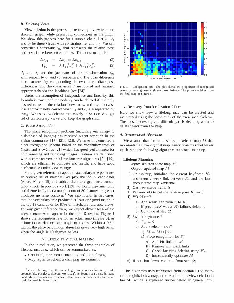
For a given reference image, the vocabulary tree generatesan ordered set of matches. We pick the topN candidates(whereN is ∼ 15) and subject them to a geometric consis-tency check. In previous work [19], we found experimentallyand theoretically that a match count of 30 features or greaterproduces no false positives.1 We also found, in test cases,that the vocabulary tree produced at least one good match inthe top 15 candidates for 97% of matchable reference views.For any given reference view, we expect almost 60% of thecorrect matches to appear in the top 15 results. Figure 1shows the recognition rate for an actual map (Figure 6), asa function of distance and angle to a view. Within a 0.5mradius, the place recognition algorithm gives very high recallwhen the angle is 10 degrees or less.

IV. L IFELONG V ISUAL MAPPING

In the introduction, we presented the three principles oflifelong mapping, which can be summarized as:

• Continual, incremental mapping and loop closing.• Map repair to reflect a changing environment.

1Visual aliasing, e.g., the same large poster in two locations, couldproduce false positives, although we haven’t yet found sucha case in manyhundreds of thousands of matches. Filters based on positional informationcould be used in these cases.

Fig. 1. Recognition rate. The plot shows the proportion of recognizedposes for varying pose angle and pose distance. The poses aretaken fromthe final map in Figure 6.

• Recovery from localization failure.

Here we show how a lifelong map can be created andmaintained using the techniques of the view map skeleton.The most interesting and difficult part is deciding when todelete views from the map.

A. System-Level Algorithm

We assume that the robot stores a skeleton mapM thatrepresents its current global map. Every time the robot wakesup, it runs the following algorithm for visual mapping.

Lifelong MappingInput: skeleton view mapMOutput: updated mapM

1) On wakeup, initialize the current keyframeKc

and insert a weak link betweenKc and the lastencountered map keyframe.

2) Get new stereo frameS3) Perform VO to get the relative poseKc ↔ S

4) VO failure?

a) Add weak link fromS to Kc

b) If previousS was a VO failure, delete itc) Continue at step (2)

5) Switch keyframes?

a) Kc ⇐ S

b) Add skeleton node?

i) M ⇐ M ∪ {S}ii) Place recognition forS?

A) Add PR links toM

B) Remove any weak linksC) Check for view deletion usingKc

D) Incrementally optimizeM

6) If not shut down, continue from step (2)

This algorithm uses techniques from Section III to main-tain the global view map; the one addition is view deletion inline 5C, which is explained further below. In general form,

Fig. 2. Sequence stitching. The robot traverses the first sequence (red),then is transported 5m and restarted (green). After continuing a short time,a correct view match inserts the new trajectory into the map.

the algorithm is very simple. Waking up, the robot is lost,and inserts a weak link to keep the map connected. Thenit processes stereo frames at 30 Hz, using VO to connecteach frame to the last. If there is a failure, it proceeds aswith wakeup, putting in a weak link. Otherwise, it tests fora keyframe addition, which happens if the match score fallsbelow a threshold, or the robot has moved a certain amount(usually 0.3m or 10 degrees). On keyframe addition, a furthercheck is made on whether to add a skeleton view, which is thesame test as for keypoint switching, with a further constraintof at least 15 frames (0.5 seconds) between skeleton views.If a skeleton view is added, it checks all views in the graphfor matches, and adds any links it finds, removing the now-unnecessary weak link. The view deletion algorithm is runon Kc (see Section V) to thin out crowded skeleton views.Finally, the graph is incrementally optimized, and the processrepeats until the robot shuts down.

B. Map Stitching

Loop closure, recovery from VO failure, and globallocalization on wakeup are handled by a uniform place-recognition mechanism. To illustrate, consider two smallsequences that overlap somewhere along their length. Thesecan represent any of the three scenarios above. In Figure2, the first sequence in red ends in a VO failure or robotshutdown. The second sequence (green) starts some 5maway, without anya priori knowledge of its relation to thefirst. The weak link (dotted line) connects the last view ofthe red sequence with the first view of the green sequence, tomaintain a connected graph. After traveling along the greensequence, PR makes matches to the first sequence. Optimiza-tion then brings the sequences into correct alignment, and theweak link can be deleted.

C. Computation and Storage

The Lifelong Mapping algorithm can be run online usinga single processor core. The time spent in view integrationis broken down by category in Figure 3. VO takes 11 msaverage per frame; there are a maximum of two skeletonsviews added per second, leaving at least 330 ms to process

Fig. 3. Timing for view integration per view during integration of the lastsequence of Figure 6.

each one. Averages for for adding to and searching thevocabulary tree are 25 ms, and for the geometry check, 65ms. Optimization by Toro in incremental mode uses less than10 ms per view.

Storage for each skeleton view consumes 60KB (average300 features at 200 bytes for the descriptor); we can easilyaccommodate 50K views in memory (3GB). With a 50m x50m building, assume that the robot’s trajectories are spreadover, say, 33% of the building’s area; then the maximumdensity of views in the map is 50 per square meter, morethan adequate for good recognition.2

V. FORGETTINGV IEWS

A robot running continuously in a closed environment willeventually accumulate enough images in its graph to stressits computational abilities. Pruning the graph is essential tolong-term viability. The question is how to prune it in a“reasonable” way, that is, what criteria guide the deletionofviews? If the environment were static, a reasonable choiceis reconstruction quality, which was successfully developedin the Photo Tourism project [25]. With a dynamic map, wewant to maximize the chance that a given view in the mapwill be used in recognizing the pose of the robot via a newview.

A. Visual Environment Types

Consider a stereo camera at a fixed position capturingimages at intervals throughout a period of time. Figure4 shows the matching evolution for different persistenceclasses. In a completely static scene, a view will continueto match all view that come after it. In a static scene withsome small changes (e.g., dishes or chairs being moved),there will be a slow degradation of the matching score overtime, stabilizing to the score for features in the static areas.If there is a large, abrupt change (e.g., a large poster moved),then there is a large falloff in the matching score. There are

2We are experimenting with just saving the vocabulary word index foreach feature as in [12], which would increase the limit to 500Kviews, anda density of 500 per square meter.

Fig. 4. View environments. On the left, a schematic of view responses overtime. Every bar represents how well a view matches subsequent views at thesame position for the given environment type. On the right, theclusters thatare induced by the environment (see Section V-D). The red circled clusteris from the original view, which does not survive in the Ephemeral case.

changes that repeat, like a door opening and closing, thatlead to occasional spikes in the response graph. Finally, acommon occurrence is an ephemeral view, caused by almostcomplete occlusion by a dynamic object such as a person– this view matches nothing subsequently. An environmentcould have a mixture of these types, for example, occlusioncan occur with any of them.

Our main idea is similar to the environment-learningstrategy of [5], which attempts to learn distinct configurationsof laser-generated local maps – for example, with a door openand closed. In our case, we want to learn clusters of viewsthat represent a similar and persistent visual environment.

B. View Clustering

To cluster views based on their recognition environment,the obvious score is the inlier match percentage. Letv andv′

be two views,m the minimum count of their two feature sets,and m the number of inliers in their match. The closenessof the two views is defined as

c(v, v′) ≡m

m− 1. (4)

The closeness measure is zero if two views match exactly,and increases to infinity when there are no matching features.Note that closeness is not a distance measure, since it doesnot obey the triangle inequality (informally, two images maybe close to a third image, but not close to each other).

The closeness measure defines the graph of the skeletonset, where an edge between two views exists ifc(v, v′) < τ

for some match thresholdτ . For a setS of views, aclusterof S is any maximal connected subset ofS.

In deleting a viewv from a clusterS, it is important toretain the connectedness of edges coming into a cluster. Ifthere is an edge(v, a) from an external nodea that has noother link to the cluster, then a new link is formed fromato a nodev′ of the cluster that is connected tov, using thetechnique of Section III-B. If the cluster is a singleton, thenall pairs of nodesa, b linked to v are connected.

C. Metric Neighborhood

While running, the robot’s views in the skeleton willseldom fall on exactly the same pose. Thus, to cluster views,we need to define aview neighborhoodηd, ηφ over whichto delete redundant views. The size of the neighborhood isdependent on the scale of the application and the statisticsofthe match data. In large outdoor maps it may be sufficient tohave a view every 10m or so; for close-up reconstruction ofa desktop we may want views every 10cm. For the typicalindoor environments of this paper, the data of Figure 1suggest thatηd = 0.5m is a reasonable neighborhood, andwe use this in the experiments of Section VI.

The view angleηφ is also important in defining the neigh-borhood, since matching views must have an overlappingFOV. Again, the data suggest a neighborhood value ofηφ =10o.

The skeleton graph induces a global 3D metric on itsnodes, but the metric is not necessarily globally accurate:as the graph distance between nodes increases, so does theirrelative uncertainty. The best way to see this is to note thatalarge loop could cause two nodes at the beginning and end ofthe loop to be near each other in the graph global pose, butnot in ground truth, if the uncertainty of the links connectingthe nodes is high. So, we search just the local graph arounda view to find views that are within its neighborhood.

D. An LRU Algorithm

Within a metric neighborhood consisting of a setS ofviews, we want to do the following:

• limit the number of views to a maximum ofκ;• preserve diversity of views;• preferentially remove older, unmatched views.

The main idea of the following view deletion algorithm isto use clusters ofS to indicate redundant views, and try topreserve single exemplars from as large a number of clustersas possible, using a least-recently used (LRU) algorithm.

LRU View DeletionInput: set ofn ≤ κ views vi in a neighborhood, a newview v, a view limit κ, and a view match thresholdτ .Output: updated set of views of size≤ κ.

• Add v to the graph• If c(v, vi) > τ for all vi (no match), set the

timestamp ofv to -1 (oldest timestamp)• While n > κ do

– If any cluster has more than one exemplar,delete the oldest exemplar among these clusters

– Else delete the oldest exemplar

E. Analysis

This algorithm obviously preserves the sparsity of viewsin a neighborhood, keeping it at or belowκ. To preserveexemplar diversity, the algorithm will keep adding viewsuntil κ is reached. Thereafter, it will add new (unmatched)views at the expense of thinning out all the clusters, untilsome cluster must be deleted. Then it chooses the oldest

Fig. 5. Representative scenes from the large office loop, showing matched features in green. Note blurring, people, cluttered texture, nearly blank walls.

Fig. 6. Trajectories from robot runs through an indoor environment. Left: four typical trajectories shown without correction. Right: the complete lifelongmap, using multiple trajectories. The map has 1228 views and 3826 connecting links. Distances are in meters.

cluster. Figure 4 shows examples of cluster evolution for thedifferent environments. In the case of static environments,there is just a single cluster, populated by the most recentviews. When there is a large change, a new cluster will growto have all the exemplars but one – should the change bereversed as in the repetition scene, that cluster will againgrow. Notice that the bias towards newer views reduces oldercluster to single exemplars in the long term.

One of the interesting aspects of the view deletion al-gorithm is how it deals with new ephemeral views. Sucha view v starts a new cluster with the oldest timestamp.The next view to be added will not matchv; assuming theneighborhood is full, and all clusters are singletons,v willbe deleted. Only if the cluster is confirmed with the nextaddition matching will it survive.

In the long term, the equilibrium configuration of anyneighborhood is a set of singleton clusters, representing themost recentκ stable environments with the most recentexemplars for each environment. This is the most desiredoutcome for any algorithm.

Our clustering algorithm has similarities to the fuzzy-means clustering done by Burgard et al. [5]. For their 2Dlaser maps, a local occupancy grid is treated as a vector, andthe vectors are clustered to find representative environments.

The number of clusters is traded off against the divergenceof each cluster using a Bayesian Information Criteria. In ourcase, we have a more direct means of comparing views, usingthe closeness measurec(v, v′). We can vary the thresholdτ to obtain different bounds on the cluster variance. Ourtechnique has the advantage of low storage requirements andan aging process to get rid of long-unused views. Finally,there is no need to choose a particular cluster for localization,as in [5], because a new view is compared against all viewsto find the best match.

Our algorithm differs from the sample-based approach ofBiber and Duckett [4], which forms clusters as randomly-chosen samples at different time scales and synthesizes thecommon features into an exemplar. Instead, we keep singlerecent exemplars for each cluster, which have a better chanceof matching new views.

VI. EXPERIMENTS

We performed a series of experiments using a robotequipped with a stereo head from Videre Design. The FOVwas approximately 90 degrees, with a baseline of 9 cm,and a resolution of 640x480. The experiments took place inthe Willow Garage building, a space of approximately 50xx 50m, containing several large open areas with movablefurniture, workstations, whiteboards, etc. All experiments

Fig. 7. Additional later sequence added to the map of Figure 6;closeup is on the left. The new VO path is in green, and the intra-path links are ingray. There are 650 views and 2,676 links in this sequence, bringing the total map to almost 2K views. All inter-path links are shown in blue. Note therelatively few links between the new path and the old ones, showing the environment has changed considerably. No view deletion is done in this figure.

were done during the day with no attempt to change theenvironment or discourage people from moving around therobot. Figure 5 shows some representative scenes from theruns.

A. Incremental Construction

Over the course of two days, we collected a set of sixsequences covering a major portion of Willow Garage. Thesequences were done without regard to forming a full loop orconnecting to each other – see the four submaps on the left ofFigure 6. There were no VO failures in the sequences, evenwith lighting changes, narrow corridors, and walls with littletexture. The map stitching result (right side, Figure 6) showsthat PR and optimization melded the maps into a consistentglobal whole. A detail of the map in Figure 8 shows thedensity of links between sequences in a stable portion of theenvironment, even after several days between sequences.

To show that the map can be constructed incrementallywithout regard to the ordering of the sequences, we redid theruns with a random ordering of the sequences, producing thesame overall map with only minor variation.

For the whole map, there were a total of 29K stereoframes, resulting in a skeleton map with 1228 view nodesand 3826 links. The timings when adding the last sequenceare given in Figure 3. Given that we run PR and skeletonintegration only at 2 Hz, timings show that the system canrun online.

B. Map Repair

After an interval of 4 days, we made an additional se-quence of some 13K frames, covering just a small 10m x5m portion of the map. During this sequence, the stereo pairwas covered at random times, simulating 20 extended VOfailures. The area was a high-traffic one with lots of movablefurniture, so the new sequence had a significantly differentvisual environment from the original sequences. The objectwas to test the system’s ability to repair a map, and do sounder adverse conditions, namely VO failures.

Fig. 8. Detail of a portion of the large map of Figure 6. The cross-linksbetween the different sequences are shown in blue.

In Figure 7, the new sequence is overlaid against theoriginal ones. Despite numerous long VO failures, the newsequence is integrated correctly and put into the right re-lation with the original map. Because the environment waschanged, there are relatively few links between the originalsequences and the new one (see the detail on the right), whilethere are very dense connections among the older sequences.In the new environment, the old sequences are no longeras relevant for matching, and the map has been effectivelyrepaired by the new sequence.

C. Deletion in a Small Area

We did not do view deletion in the first experiment becausethe density of views was not sufficient to warrant it. With thesmall area sequence just presented, there were enough viewsto make deletion worthwhile. We collected statistics on themap with different values forκ, the maximum number ofviews allowed in a neighborhood. These statistics are for the

area occupied by the new sequence.

κ ∞ 7 5 4 3 2Views 643 232 162 134 104 78Edges 2465 361 213 184 293 269

Views/nb 17.7 6.1 4.6 3.8 2.9 2.0Clusters/nb 2.0 2.3 2.1 2.0 1.8 1.5

The View line shows the total number of new views in themap, which decrease significantly withκ. New edges alsodecline untilκ = 4, and which point more edges are neededas clusters are deleted and their neighbors must be linked.

The most interesting line is clusters per neighborhood. Ingeneral, there are two clusters, one for each direction therobot traverses along a pathway – views from these directionshave no overlapping FOV. Note that decreasingκ keeps thenumber of clusters approximately constant, while reducingthe number of views substantially. It is the clusters thatpreserve view diversity.

VII. C ONCLUSION

We believe this paper makes a significant step towardsa mapping system that is able to function for long periodsof time in a dynamic environment. One of the main contri-butions of the paper is to present the criteria for practicallifelong mapping, and show how such a system can bedeployed. The key technique is the use of robust visual placerecognition to close loops, stitch together sequences madeatdifferent times, repair maps that have changed, and recoverfrom localization failures, all in real time. To operate inlarger environments, it is also necessary to build a realtime,optimized map structure connecting views, a role filled bythe skeleton map and Toro.

The role of view deletion in maintaining an efficient maphas been highlighted. With the LRU deletion algorithm, wehave shown that exemplars of different environments can bemaintained in a fine-grained manner, while minimizing thestorage required for views.

One of the main limitations of the paper is the lack of long-term data and results on how the visual environment changes,and how to maintain matches over long-term changes. Not allfeatures are stable in time, and picking out those that are isagood idea. We have begun exploring the use of linear featuresas key matching elements, since indoors the intersection ofwalls, floors and ceilings are generally stable.

VIII. ACKNOWLEDGMENTS

We would like to thank Giorgio Grisetti and Cyrill Stach-niss for providing Toro, and for their help in getting theincremental version to work. We also would like to thankMichael Calonder and Patrick Mihelich for their work onthe place recognition system.

REFERENCES

[1] M. Agrawal and K. Konolige. Rough terrain visual odometry. In Proc.International Conference on Advanced Robotics (ICAR), August 2007.

[2] M. Agrawal and K. Konolige. FrameSLAM: From bundle adjustmentto real-time visual mapping.IEEE Transactions on Robotics, 24(5),October 2008.

[3] H. Andreasson, A. Treptow, and T. Duckett. Self-localization in non-stationary environments using omni-directional vision.Robotics andAutonomous Systems, 55(7):541–551, July 2007.

[4] P. Biber and T. Duckett. Dynamic maps for long-term operation ofmobile service robots. InRSS, 2005.

[5] W. Burgard, C. Stachniss, and D. Haehnel. Mobile robot maplearningfrom range data in dynamic environments. InAutonomous Navigationin Dynamic Environments, volume 35 ofSpringer Tracts in AdvancedRobotics. Springer Verlag, 2007.

[6] J. Callmer, K. Granstrom, J. Nieto, and F. Ramos. Tree of words forvisual loop closure detection in urban slam. InProceedings of the2008 Australasian Conference on Robotics and Automation, page 8,2008.

[7] M. Calonder, V. Lepetit, and P. Fua. Keypoint signaturesfor fastlearning and recognition. InECCV, 2008.

[8] M. Cummins and P. M. Newman. Probabilistic appearance basednavigation and loop closing. InICRA, 2007.

[9] F. Dayoub and T. Duckett. An adaptive appearance-based map forlong-term topological localization of mobile robots. InIROS, 2008.

[10] E. Eade and T. Drummond. Unified loop closing and recovery for realtime monocular slam. InBMVC, 2008.

[11] D. Fox and W. Burgard. Markov localization for mobile robots indynamic environments.Journal of Artificial Intelligence Research,11:391–427, 1999.

[12] F. Fraundorfer, C. Engels, and D. Nister. Topological mapping,localization and navigation using image collections. InIROS, pages3872–3877, 2007.

[13] G. Grisetti, C. Stachniss, S. Grzonka, and W. Burgard. Atreeparameterization for efficiently computing maximum likelihoodmapsusing gradient descent. InIn RSS, 2007.

[14] J. Gutmann and K. Konolige. Incremental mapping of large cyclicenvironments. InProc. IEEE International Symposium on Computa-tional Intelligence in Robotics and Automation (CIRA), pages 318–325, Monterey, California, November 1999.

[15] D. Haehnel, R. Triebel, W. Burgard, and S. Thrun. Map building withmobile robots in dynamic environments. InICRA, pages 1557–1563,2003.

[16] H. Jegou, M. Douze, and C. Schmid. Hamming embedding and weakgeometric consistency for large scale image search. InECCV, 2008.

[17] H. Jegou, H. Harzallah, and C. Schmid. A contextual dissimilaritymeasure for accurate and efficient image search.Computer Vision andPattern Recognition, IEEE Computer Society Conference on, 0:1–8,2007.

[18] K. Konolige and M. Agrawal. Frame-frame matching for realtimeconsistent visual mapping. InProc. International Conference onRobotics and Automation (ICRA), 2007.

[19] K. Konolige, J. Bowman, J. Chen, P. Mihelich, M. Colander, V. Lepetit,and P. Fua. View-based maps. InSubmitted, 2009.

[20] M. Montemerlo and S. Thrun. Conditional particle filtersfor simulta-neous mobile robot localization and people-tracking. InICRA, pages695–701, 2002.

[21] D. Nister and H. Stewenius. Scalable recognition with a vocabularytree. InCVPR, 2006.

[22] E. Rosten and T. Drummond. Machine learning for high-speed cornerdetection. InEuropean Conference on Computer Vision, volume 1,2006.

[23] J. Sivic and A. Zisserman. Video google: A text retrievalapproachto object matching in videos.Computer Vision, IEEE InternationalConference on, 2:1470, 2003.

[24] R. C. Smith and P. Cheeseman. On the representation and estimationof spatial uncertainty. International Journal of Robotics Research,5(4), 1986.

[25] N. Snavely, S. M. Seitz, and R. Szeliski. Skeletal sets for efficientstructure from motion. InProc. Computer Vision and Pattern Recog-nition, 2008.

[26] I. Ulrich and I. Nourbakhsh. Appearance-based place recognition fortopological mapping. InICRA, 2000.

[27] C. Valgren, A. Lilienthal, and T. Duckett. Incremental topologicalmapping using omnidirectional vision. InIROS, 2006.

[28] B. Williams, G. Klein, and I. Reid. Real-time slam relocalisation. InICCV, 2007.

[29] D. Wolf and G. Sukhatme. Online simultaneous localization andmapping in dynamic environments. InICRA, 2004.