Towards The Modeling Of Simulated Inflows into Lake Powell Andrew Laird

September 29, 2014 !Introduction !

Lake Powell is the second largest reservoir in the United States with a capacity of approximately 26.2 million acre-feet (maf). It was created by the damming of the Colorado and San Juan rivers with the Glen Canyon Dam in 1963. The dam enables the generation of hydroelectric power and regulates water flows to the downstream states of Arizona, Nevada, and California as established by the Colorado River Compact (USBR, 1922). The reservoir extends 299 km from the inflow to the dam, with depths as great as 168 meters at the deepest points immediately before the dam (Gloss et al., 2005). The damming of these rivers has a significant impact on the upstream and downstream ecology of the river system, and the Grand Canyon Protection Act of 1992 mandates that the outflow water quality and volume be monitored and controlled in order to prevent adverse impacts downstream from the dam (USBR, 2008). In 2005, Susan Hueftle of the Grand Canyon Monitoring and Research Center showed that a plume of water with low dissolved oxygen (DO) levels passed through the lake, out the penstocks of the dam, and into the downstream ecosystem without being mixed with more oxygenated water. This resulted in the release of hypoxic water into the downstream ecosystem. Water low in DO is known to have negative consequences on ecosystem health, particularly over sustained periods. Hueftle’s data showed that this period of low-DO outflows lasted from approximately late August through mid-November before the annual convective vertical circulation drew the relatively warm deep water upwards to displace the cooling surface waters, thus mixing the water column of the reservoir (Hueftle, 2005). Despite the known negative impact of low-DO events on ecosystem health, there is still limited understanding of the factors which influence dissolved oxygen levels in the lake or the hydrodynamic characteristics that must be present for low-DO waters to reach the dam. Presently, there are two proposed hypotheses that seek to explain the causes of reduced DO levels within the lake. Each provides for the loss of oxygen from lake inflows through chemical interactions with lake sediment that has been resuspended in the water by inflows to the reservoir (Hueftle, 2005; Williams, 2007). When snowmelt occurs in the Colorado River watershed, the water feeds into the river, increasing river flow volume substantially in the spring, meaning that a substantial amount of sediment can be displaced by snowmelt-driven spring inflows. Although these chemical interactions are beyond the scope of this study, they are only one component of what is required for low-DO dam outflows. At least as important are the physical processes of the lake that transport the plume from its source to the penstocks. This study focused primarily on these transport processes in an attempt to identify the lake dynamics like total inflow volume, inflow rate, and water level that promote the transfer of low DO plumes into the downstream ecosystem. Unfortunately, due to the variability of conditions in the natural environment, it is prohibitively difficult to test these processes in the reservoir. To combat this, this study will employ CE-QUAL-W2 modeling software developed by the US Army Corps of Engineers and Portland State University. The software, used in conjunction with a template specifically designed to provide simulation information about Lake Powell, allows the user to simulate water flow through the reservoir based on specified meteorological and hydrological factors and simulate 21 chemicals and chemical processes including, most notably, concentrations of DO throughout the lake. Modifying various aspects of the input data

allows the user to see how these factors impact the reservoir over time. Running a simulation using the CE-QUAL-W2 model requires developing large, data-rich input files and results in the creation of output files containing tens of thousands of values representing the state of the reservoir over the course of the simulation. As these volumes of data are too large to be reasonably processed by hand (i.e., in Microsoft Excel), additional software must be employed to create the inflow data series and analyze the output data and provide answers to the questions set out in this study. This provides an excellent opportunity to employ the programming language Python. Python is a general purpose programming language which has gained a strong following in scientific computing as a result of the creation of libraries such as NumPy, SciPy, Matplotlib, Statsmodels, and pandas. Within the context of programming, libraries are related collections of pre-made code designed to allow programmers to apply existing tools to their projects without having to develop each piece of code from scratch. The above libraries provide powerful data processing, formatting, and display tools which can be applied with relative ease to large data sets. These libraries were used both in the preparation of the input files necessary to run simulations and in the analysis and presentation of output data. As this project has evolved, it has become clear that there are three distinct phases involved in modeling transport processes in order to see which variables have the greatest impact on the creation and persistence of low dissolved oxygen plumes in the Glen Canyon Dam. These phases are the preparation of model input data, the modeling process itself, and the investigation of the output data to identify trends in the variables. As this is an ongoing project, this report will focus mainly on the initial phase of the project, which was the primary subject of my work over the course of the Summer Fellowship period, as well as providing some insight into the initial aspects of the modeling process. In order to run the CE-QUAL-W2 model, the user must provide many variables to the model that define the state of the model both initially and throughout the process. The model user inputs data and constants from which reservoir conditions at each time step (usually 1 day) are calculated using a series of mass- and momentum-balance equations. Fortunately, many constants were determined by Nick Williams of the U.S. Bureau of Reclamation, the engineer who developed and calibrated the model. The study involved alteration of some model inputs, and the bulk of the Python programming which was done over the summer was done to develop these input files. The primary driver of many reservoir characteristics is the inflow from the Colorado River, which can vary substantially from day to day, season to season, and year to year. This report will detail the work that was done in developing both the inflow data itself as well as the inflow files, and it will look at how these files will be used in modeling reservoir variables as research continues. !

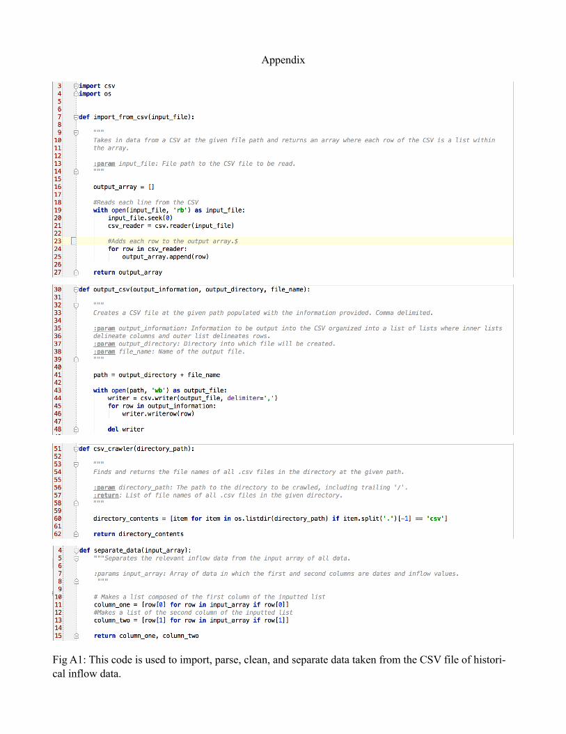
Methods ! We hypothesize that a large spring inflow into a reservoir with a low water surface elevation caused by several consecutive low-inflow years may have been responsible for the magnitude and duration of the low-DO plume that was observed in 2005. In order to test this hypothesis, a number of input files were created with varying inflow scenarios that will be used as inputs to the model. Subsequently, the model results will be evaluated to identify the progression of a low-DO plume to the penstocks of the dam. The initial objective when developing these inflow input files was to create an algorithm through which a random spring inflow could be generated. To do this, the first step was to identify the spring inflow periods for each year in the historical inflow data, which spans from water year (WY) 1963 to WY2013, and quantify variables that could be used to create realistic simulated inflows. The code

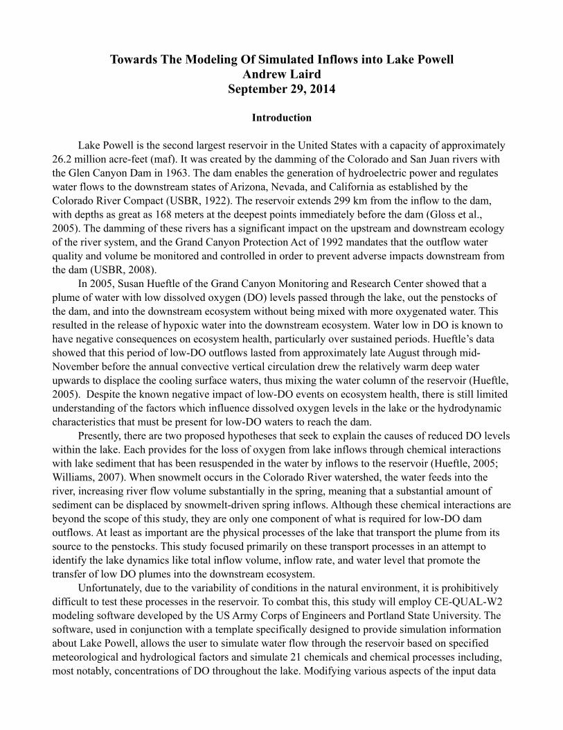
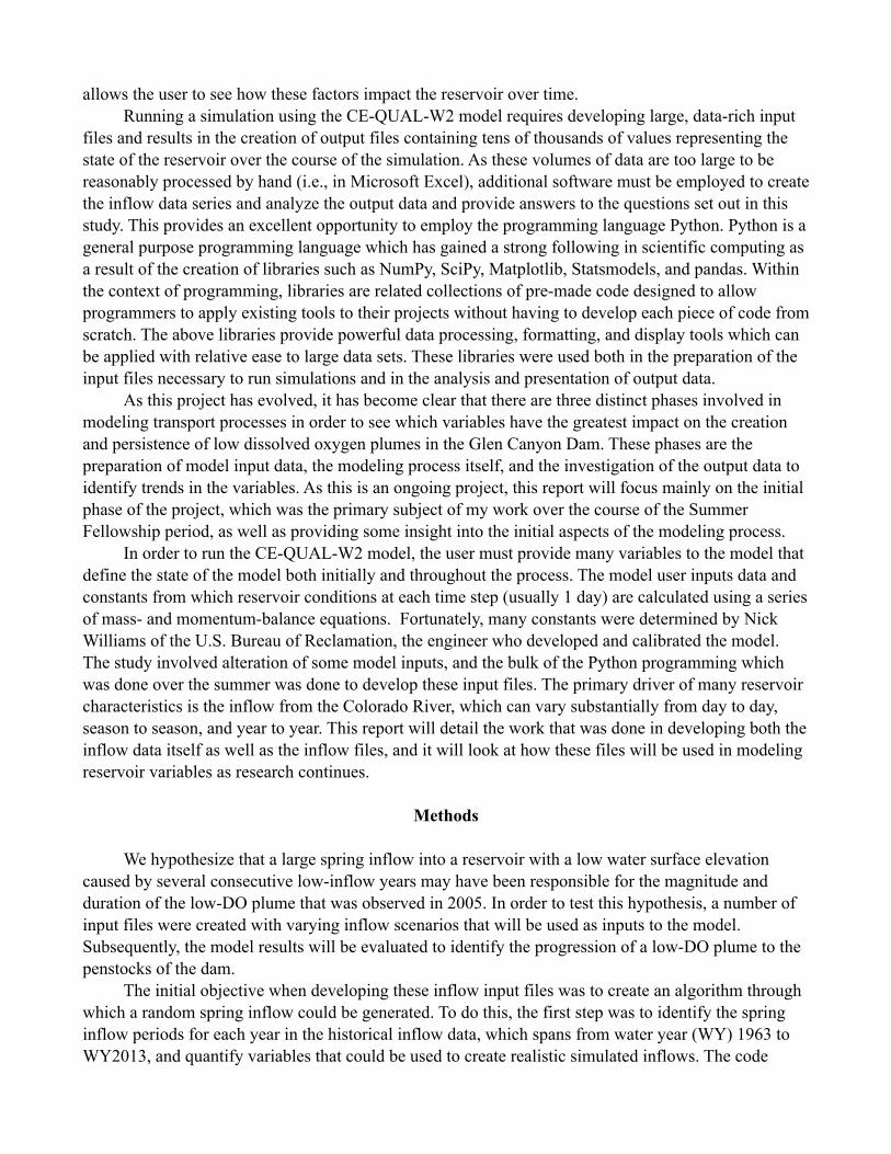
which was used to import, clean, and separate the data by year from the original CSV file can be seen in Fig A1 (A denotes that a figure appears in the appendix). Importing of data is relatively self explanatory, in that it means bringing the data into the Python program from the CSV file in which it originated, allowing it to be manipulated programmatically. Unfortunately, many data files are designed with human readability in mind rather than for consumption by computers which are actually hindered rather than aided by additional spacing and explanatory text. This means that the data must be cleaned or “wrangled” as the process is sometimes called in order to allow the computer to read in the values as the user would expect. In this case, this process included converting values from string (text) values into float (numerical) values and eliminating several lines of explanatory text from the header of the document, in addition to several other minor tasks. The final step was to break up the data by separating each year into an individual component of the historical data, in addition to separating the data which we were concerned with, namely the date and Colorado River inflow elements, from the overall data table which included inflow values for a number of additional tributaries which are not currently relevant to the study. Identifying the spring period of an inflow year is simple in some years and difficult in others. This is because the spring inflow of the Colorado River is driven by snow melt from the Rocky Mountains, and thus the inflow's characteristics hinge on the quantity and melt rate of this snow. During a normal year, snowmelt causes a substantial change in the rate of water flowing in from the Colorado River during the spring as compared with the rest of the year. While inflow volumes rarely exceed 10,000 cfs outside of the spring period, flow rates can reach and exceed 60,000 cfs in the spring months of a normal water year and have reached historic highs greater than 150,000 cfs. Low snow volumes or melting during the winter months can reduce the size of the spring inflows substantially, however, and cause the inflow rates during the spring to be indistinct from those of the rest of the year. This variability poses a significant challenge in modeling the river's inflow behavior because the range of possible values for inflow entries vary so broadly that it is hard to define clearly whether the inflow on a given day is part of the spring inflow for that year. Fig 1a shows an example of an inflow period from what could be considered a typical year, while Fig 1b shows the inflow from a drought or low inflow year.

![Fig 1a (left) is an example graph showing the inflow volume over time for a typical inflow year (WY2004). The figure was generated using the matplotlib and pandas libraries for Python. Fig 1b (right) depicts an example inflow from a low water year (WY1976).]

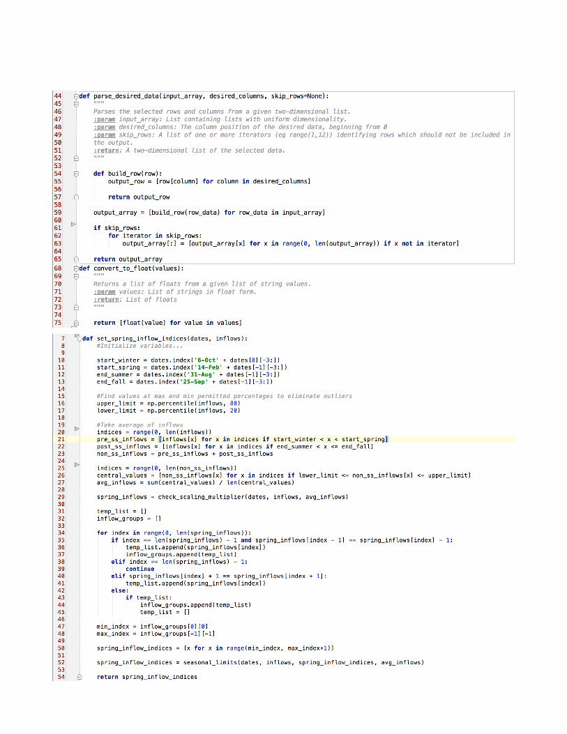
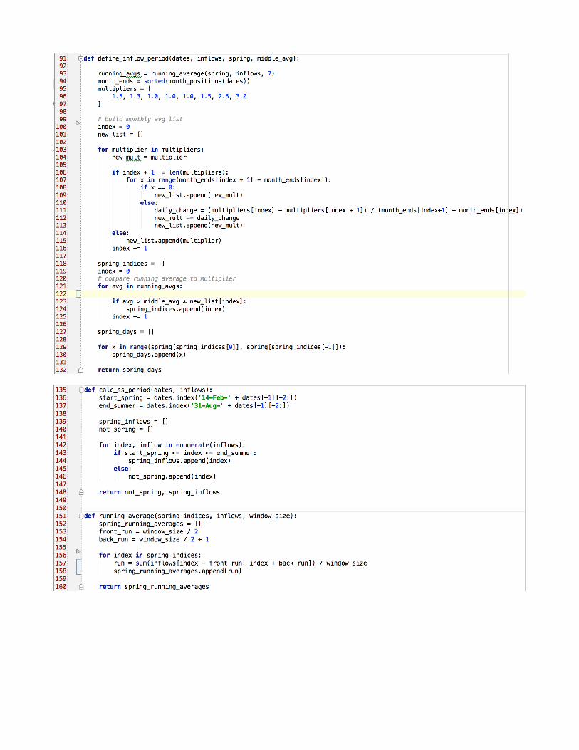
! In order to address this problem, I developed an algorithm that would capture the inflow in all cases. This algorithm has two eventual implementations that can be seen in Fig A2 and Fig A3, although the second implementation is currently incomplete. The general objective of the algorithm is to take in a series of observed inflow values and identify those that could belong to the spring period based on their magnitude relative to the size of the inflows during the 'non-spring' period, which was defined as the period from October 1st, the beginning of the water year, to Feb 14th, and from August 31st to September 30th, the end of the water year. There are several constraints which must be addressed in selecting a spring inflow period. The period must be contiguous – this means that the algorithm cannot select a peak early in the year and then include a lengthy period of base inflows before the true spring period begins. Additionally, the spring period cannot begin before February 14th or continue beyond August 31st. High inflow values outside these times are attributable to other factors such as runoff from large storms, and thus should not be included in the spring inflows. The code in Fig A3 shows how the spring period was defined. The code simply identifies the dates in the inflow file which correspond to the relevant dates for the spring period through string matching and creates two separate multi-dimensional lists containing the data for the spring and non-spring periods. This makes future execution of code on these two groups of data more straightforward. With these two groups separated, it is possible to find a good baseline value for the non-spring flow. To do this, I computed the mean of the values between the 20th and 80th percentiles of the non-spring data. I choose to eliminate the largest and smallest values because, in some low inflow years, storms can cause significant variation in the data and make it more difficult to distinguish between the typical flow for the year and the spring values. This mean plus a percentage is then compared to a computed 7 day running average value for each day of the spring period. The spring is defined as beginning when the running average exceeds the mean plus the added percentage. The added percentage varies over the course of the spring months such that the running average must be greater at the extreme ends of the spring months for those dates to be considered spring inflows, while the added percentage is lower towards the middle of the spring dates as these are more likely to be spring inflows even if they have lower values. These values vary by day over the course of the spring and summer, and their computation can be seen in Fig A2. Once the spring inflow period has been identified for each year, variables pertaining to the inflow's characteristics can be computed. The variables which were selected are kurtosis, skewness, total inflow volume, and start date. These variables were computed using the Scipy and numpy libraries for Python using built-in functions and basic computations, which summed daily average inflow values into a total inflow value for the season. The code used for these computations can be seen in Figure A4. The original objective was to use these variables to generate random realistic values for simulated inflow years. Unfortunately, due to time constraints and a lack of necessary statistical background, I was unable to generate the intended simulated inflow years during the Fellowship period. This is due to the fact that knowing the four moments of a distribution - mean, variance, skewness, and kurtosis - is not sufficient to generate an exclusive distribution as there are multiple distributions for which these values can be the same. There are several formulas which seek to generate a guess at the intended distribution, including some built into the Scipy library, however I was unable to generate realistic results after several attempts to employ these tools. With further research, it's possible that these inflows could be created, allowing for an increased range of variability and a greater number of potential simulations. In order to continue the project without developing simulated inflows, I was forced to come up

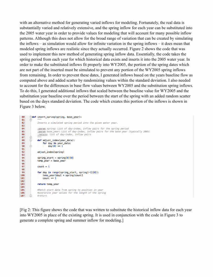
with an alternative method for generating varied inflows for modeling. Fortunately, the real data is substantially varied and relatively extensive, and the spring inflow for each year can be substituted into the 2005 water year in order to provide values for modeling that will account for many possible inflow patterns. Although this does not allow for the broad range of variation that can be created by simulating the inflows – as simulation would allow for infinite variation in the spring inflows – it does mean that modeled spring inflows are realistic since they actually occurred. Figure 2 shows the code that was used to implement this new method of generating spring inflow data. Essentially, the code takes the spring period from each year for which historical data exists and inserts it into the 2005 water year. In order to make the substituted inflows fit properly into WY2005, the portion of the spring dates which are not part of the inserted must be simulated to prevent any portion of the WY2005 spring inflows from remaining. In order to prevent these dates, I generated inflows based on the years baseline flow as computed above and added scatter by randomizing values within the standard deviation. I also needed to account for the differences in base flow values between WY2005 and the substitution spring inflows. To do this, I generated additional inflows that scaled between the baseline value for WY2005 and the substitution year baseline over the period between the start of the spring with an added random scatter based on the days standard deviation. The code which creates this portion of the inflows is shown in Figure 3 below.

![Fig 2: This figure shows the code that was written to substitute the historical inflow data for each year into WY2005 in place of the existing spring. It is used in conjunction with the code in Figure 3 to generate a complete spring and summer inflow for modeling.] !!!!!!

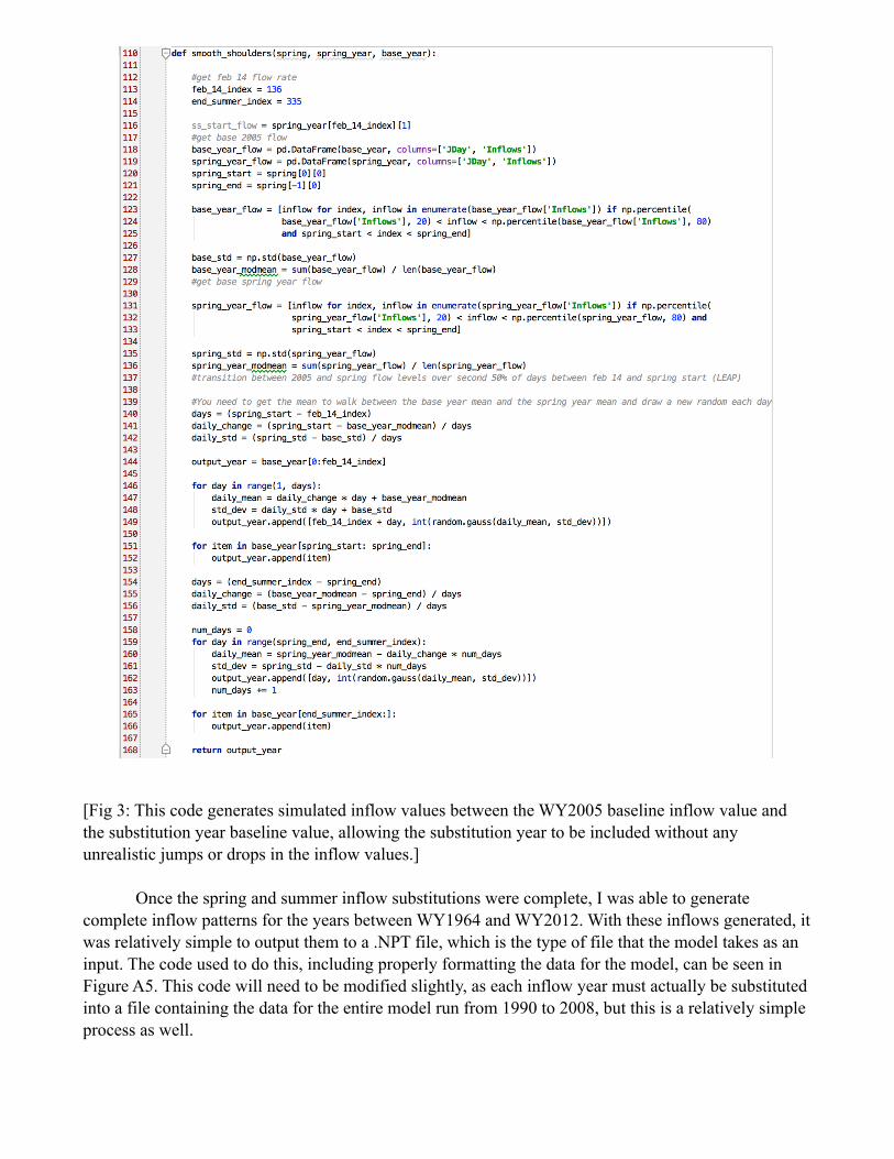
[Fig 3: This code generates simulated inflow values between the WY2005 baseline inflow value and the substitution year baseline value, allowing the substitution year to be included without any unrealistic jumps or drops in the inflow values.] ! Once the spring and summer inflow substitutions were complete, I was able to generate complete inflow patterns for the years between WY1964 and WY2012. With these inflows generated, it was relatively simple to output them to a .NPT file, which is the type of file that the model takes as an input. The code used to do this, including properly formatting the data for the model, can be seen in Figure A5. This code will need to be modified slightly, as each inflow year must actually be substituted into a file containing the data for the entire model run from 1990 to 2008, but this is a relatively simple process as well. !

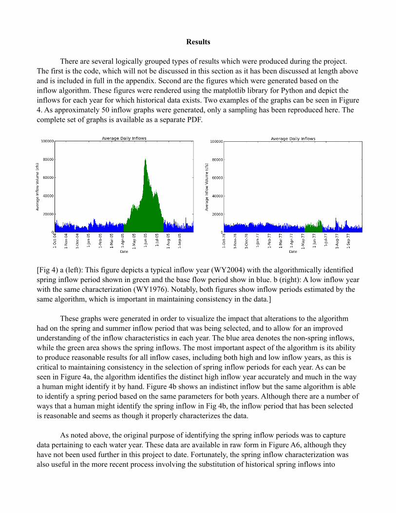
Results ! There are several logically grouped types of results which were produced during the project. The first is the code, which will not be discussed in this section as it has been discussed at length above and is included in full in the appendix. Second are the figures which were generated based on the inflow algorithm. These figures were rendered using the matplotlib library for Python and depict the inflows for each year for which historical data exists. Two examples of the graphs can be seen in Figure 4. As approximately 50 inflow graphs were generated, only a sampling has been reproduced here. The complete set of graphs is available as a separate PDF.

[Fig 4) a (left): This figure depicts a typical inflow year (WY2004) with the algorithmically identified spring inflow period shown in green and the base flow period show in blue. b (right): A low inflow year with the same characterization (WY1976). Notably, both figures show inflow periods estimated by the same algorithm, which is important in maintaining consistency in the data.] These graphs were generated in order to visualize the impact that alterations to the algorithm had on the spring and summer inflow period that was being selected, and to allow for an improved understanding of the inflow characteristics in each year. The blue area denotes the non-spring inflows, while the green area shows the spring inflows. The most important aspect of the algorithm is its ability to produce reasonable results for all inflow cases, including both high and low inflow years, as this is critical to maintaining consistency in the selection of spring inflow periods for each year. As can be seen in Figure 4a, the algorithm identifies the distinct high inflow year accurately and much in the way a human might identify it by hand. Figure 4b shows an indistinct inflow but the same algorithm is able to identify a spring period based on the same parameters for both years. Although there are a number of ways that a human might identify the spring inflow in Fig 4b, the inflow period that has been selected is reasonable and seems as though it properly characterizes the data. ! As noted above, the original purpose of identifying the spring inflow periods was to capture data pertaining to each water year. These data are available in raw form in Figure A6, although they have not been used further in this project to date. Fortunately, the spring inflow characterization was also useful in the more recent process involving the substitution of historical spring inflows into

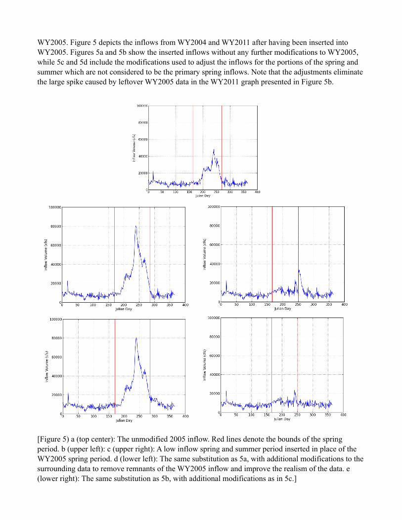
WY2005. Figure 5 depicts the inflows from WY2004 and WY2011 after having been inserted into WY2005. Figures 5a and 5b show the inserted inflows without any further modifications to WY2005, while 5c and 5d include the modifications used to adjust the inflows for the portions of the spring and summer which are not considered to be the primary spring inflows. Note that the adjustments eliminate the large spike caused by leftover WY2005 data in the WY2011 graph presented in Figure 5b.

[Figure 5) a (top center): The unmodified 2005 inflow. Red lines denote the bounds of the spring period. b (upper left): c (upper right): A low inflow spring and summer period inserted in place of the WY2005 spring period. d (lower left): The same substitution as 5a, with additional modifications to the surrounding data to remove remnants of the WY2005 inflow and improve the realism of the data. e (lower right): The same substitution as 5b, with additional modifications as in 5c.]

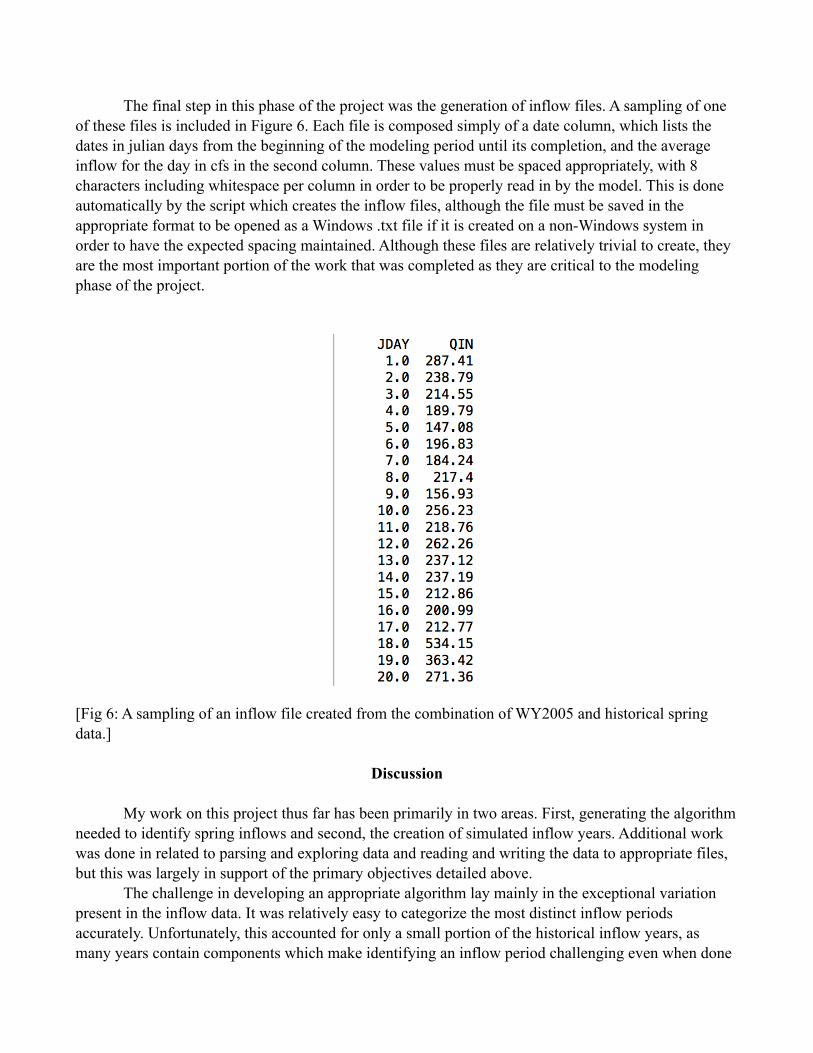
! The final step in this phase of the project was the generation of inflow files. A sampling of one of these files is included in Figure 6. Each file is composed simply of a date column, which lists the dates in julian days from the beginning of the modeling period until its completion, and the average inflow for the day in cfs in the second column. These values must be spaced appropriately, with 8 characters including whitespace per column in order to be properly read in by the model. This is done automatically by the script which creates the inflow files, although the file must be saved in the appropriate format to be opened as a Windows .txt file if it is created on a non-Windows system in order to have the expected spacing maintained. Although these files are relatively trivial to create, they are the most important portion of the work that was completed as they are critical to the modeling phase of the project.

[Fig 6: A sampling of an inflow file created from the combination of WY2005 and historical spring data.] !

Discussion ! My work on this project thus far has been primarily in two areas. First, generating the algorithm needed to identify spring inflows and second, the creation of simulated inflow years. Additional work was done in related to parsing and exploring data and reading and writing the data to appropriate files, but this was largely in support of the primary objectives detailed above. The challenge in developing an appropriate algorithm lay mainly in the exceptional variation present in the inflow data. It was relatively easy to categorize the most distinct inflow periods accurately. Unfortunately, this accounted for only a small portion of the historical inflow years, as many years contain components which make identifying an inflow period challenging even when done

manually. This difficulty was compounded by initial unfamiliarity with the Python tools best suited for testing and visualizing possible options, although this improved rapidly as scripts were developed which made handling the specific data used in this project simpler. In dealing with the most difficult inflow years, I developed several techniques which are outlined above and in the code which made categorizing difficult inflows more simple. The key realization here was that these techniques also dealt with the simple inflow cases with ease. In the future, initial focus on the more difficult edge cases rather than finding a solution that worked in many but not all cases seems as though it may have generated results more quickly as substantial effort was devoted to manipulating code designed to solve the more obvious cases into code that was capable of identifying these edge cases when the reverse may have allowed more clarity of thought with regards to the challenges posed by the most difficult cases. The second substantial portion of the project, the development of inflow years, proved difficult for different reasons. Although traversing and manipulating the data was made much easier through improved understanding of the Python tools being used by the time I arrived at this portion of the project, a new set of mathematical challenges was posed by attempting to simulate inflows. The most difficult aspect of the project actually proved to be the statistical questions posed by attempting to simulate inflows. Advanced techniques in statistics which were beyond the scope of my present understanding caused delays in creating inflows that could be modeled, and, although resources were available that seemed to describe the process by which these inflows could be generated, they were often discussed at a level that was prohibitively difficult to understand given the time constraints and objectives of the project by the time I encountered these challenges. Unfortunately, this led to a substantial portion of the work that was done over the course of the Fellowship being abandoned in favor of a more direct solution in the form of inflow substitution. Although it is possible that this work could be revisited later, it is unclear that it will be necessary in order to gain the necessary understanding needed to address the hypothesis being explored. This leads me to believe that a simpler strategy for generating inflows may have proved more useful from the outset of the project, allowing me to progress further with the modeling and analysis portions of the project. Considering alternative methods for building inflows was an area that did not receive much attention relative to the scope of the project, and likely would have been an area worth investigating not only before I began my work but also as the project advanced. The results laid out above represent the completion of the initial stage of the broader project with the exception of the inflow values being substituted into complete inflow files to allow them to be modeled properly. Although this is less progress than I had intended to make towards the overall result of the project, it does set-up the project well going forward towards the modeling and data analysis phases. The modeling process thus-far appears to be far more straightforward – if time consuming - than the initial portion of the project, although it's possible that unforeseen difficulties will arise as they have previously. The next portion of the project involves picking which years will be modeled in order to achieve a range of data that allows for testing of the current hypothesis that the low-DO inflows were driven by sediment resuspension cause by high volume inflows into a reservoir with low surface water elevation. There are presently approximately 50 inflow input files available, although others can be created by manipulating the start dates of a given years inflow period to change when in the year it occurs, leading to a much greater range of possible variation should it be deemed that more simulation data is needed. If there are insufficient data available even with these changes – an unlikely possibility – it will be necessary to revisit the original objective of simulating inflows fully from observed variable data. Although this process was abandoned, there were some indications that it was possible to generate

curves in this manner. Research also suggested that there may be other methods available for generating time series data for modeling purposes, although it was unclear whether this would require additional or alternative characterizations of the historical data. There is also an opportunity for scripting to be done in support of the modeling process which did not end up fitting within the scope of my Summer Fellowship project. Code to enable the easy swapping of inflow files into and out of the appropriate directories and to automatically move and store generated output files from the model will be highly beneficial in streamlining the modeling process going forward and is worth addressing before the modeling process begins in earnest. In addition, code for querying and modifying the control file of the model and its documentation would benefit future modeling efforts, although it is unlikely to be necessary for the modeling needed in this portion of the project. Finally, there is significant opportunity to develop code to obtain and visualize information from the output files generated by the model which has not yet been addressed. The original goal was to build this code during the modeling phase, however, since very little modeling was done during the fellowship period, this portion of the project has yet to be addressed. I am confident that additional understanding of Python tools and the existing code library will make this a more straightforward process than developing the input files, but it will still pose challenging as it requires a depth of understanding of the model's output files that I do not yet possess. It's likely that this code should be addressed once only a few model runs are completed in order to ensure that the available data from the model runs is able to fully address the questions posed by the hypothesis. Ultimately, the project is progressing reasonably well, with some of the initial major hurdles overcome, however clumsily. There is still a significant amount of work to be done to produce useful results, but I am hopeful that these aspects of the project will prove more straightforward than the work that has preceded them. !

References US Bureau of Reclamation. (1922) Colorado River Compact [PDF]. http://www.usbr.gov/lc/region/g1000/pdfiles/crcompct.pdf Gloss, S.P., Lovich, J.E., and Melis, T.S., eds., 2005, The state of the Colorado River ecosystem in Grand Canyon: U.S. Geological Survey Circular 1282, 220 p. Hueftle, S. 2005. Lake Powell Limnology. Oral presentation at the Lake Powell Cooperators Group Meeting, 6 December 2005, Page, Ariz. Miller, J.B. 2005. CE-QUAL-W2 Modeling, Calibration, and Verification for Salinity, Nutrients, Al gae, and Dissolved Oxygen spanning the time period 1990-2002. Oral presentation at the Lake Powell Cooperators Group Meeting, 6 December 2005, Page, Ariz. Williams, N.T. (2007). Modeling dissolved oxygen in Lake Powell using CE-QUAL-W2. Brigham Young University masters thesis. !!!!!!!!!!

Appendix

Fig A1: This code is used to import, parse, clean, and separate data taken from the CSV file of histori-cal inflow data.

!!

!Fig A2: This is the initial code used to calculate spring inflow periods for each year. !!!!

!!!!!!

Fig A3: This is the updated code used to calculate the spring inflow period for each year.

Fig A4: This code is used to calculate the variable values for each of the variables which was identified as necessary to compute simulated inflow distributions. The variables are kurtosis, skewness, total in-flows, and start date. !!!

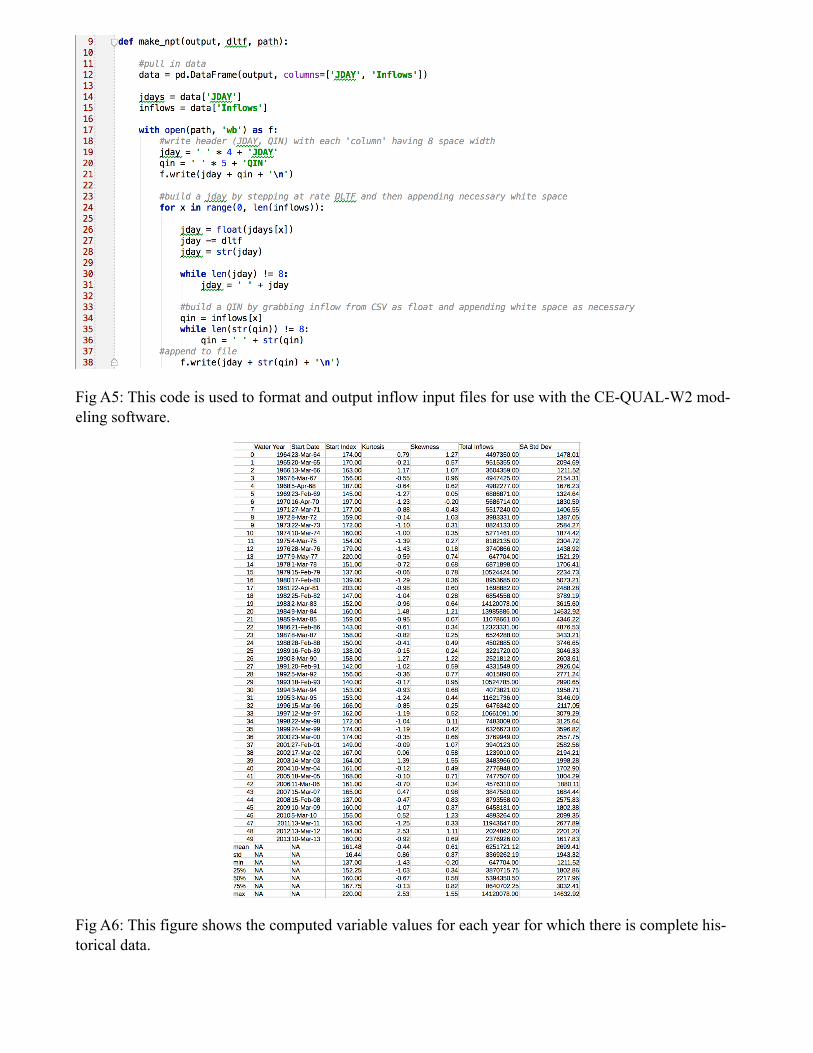
Fig A5: This code is used to format and output inflow input files for use with the CE-QUAL-W2 mod-eling software.

Fig A6: This figure shows the computed variable values for each year for which there is complete his-torical data.