Track Geometry Measurement Database and Calculation of Equivalent

Conicities of the OBB Network

DI W. Hanreich1, Dr. P. Mittermayr2, Dr. G. Presle1

1) Austrian Federal Railways, Permanent Way, Zieglergasse 7, A-1070 Wien, Austria/Europe

2) Bureau of Applied Mechanics and Mathematics, Dr. Mittermayr & Partner KEG, Lambrechtgasse 4/2,

A-1040 Wien, Austria/Europe

ABSTRACT

The track geometry recording coach EM250 of the Austrian Railways (OBB) measures track geometry space

curves at speeds of up to 160 mph. Two Inertial Measurement Systems including dGPS navigation record the

track geometry with a sampling rate of 0.25 m, and the rail profiles while at the same time analyzing rail wear

and equivalent conicities.

The enormous amount of data collected from the entire railroad network is standardized and loaded in a

huge database. Currently, several hundred workstations within the OBB can access Track Quality Indices as well

as any of the measured parameters for any specific point of interest using an Intranet application. Thus,

permanent way maintenance programs can be easily developed based on objectively measured data.

The paper includes the latest results of statistical surveys on accuracy and repeatability on the measured

parameters which were retrieved from multiple measurements conducted on the same track at different speeds

and vehicle orientations.

Furthermore, representative distributions of equivalent conicity over long measurement distances will

be presented. The data were collected on several thousand miles of the Austrian railroad’s network in a

measurement campaign conducted since the beginning of 2001.

1 THE DATA COLLECTOR: THE AUSTRIAN TRACK GEOMETRY MEASUREMENT COACH EM250

The Austrian track testing and recording coach EM250 is based on a normal passenger coach and is equipped

with 2 inertial measuring systems, a laser gage measuring system and a laser rail profile measurement system

(see Figure 1). All systems work without rail contact on an optical basis. The measurement car records and stores

the track quality at speeds of up to 250 km/h (nearly 160 mph). Track geometry measurements are taken every

25 centimeters (approx. 10 inches). Every 10 m (approx. 30 feet) rail profiles consisting of more than 500 points

for each rail head are taken and are analyzed online for wear and equivalent conicity. The correct identification

of the measurement location in terms of milepost and offset is done by an onboard navigation system which uses

differential GPS information. A GPS position with an average accuracy of less than half a meter (approx. 20

inches) is allocated to each data record. Over the past 9 years, more than 89 GByte data were recorded and

stored.

2 THE DATAWAREHOUSE: THE TRACK GEOMETRY MEASUREMENT DATABASE

In the past, the track geometry recording coach measured the tracks and stored the resulting binary data in a file

structure. However, it is difficult to search for specific measurement data in a specific location. On the other

hand there existed a database which contained the network topology and permanent way features like type of rail

and type of sleepers. The link between the measurement data and the database required an automatic generation

of a small database containing the actual topology of the network which includes all lines, intersections between

lines, number of tracks on a line and other data such as the maximum permissible speed and more than 1,000

GPS synchronization points. The content of this small database is transferred via a wireless LAN to the record-

ing coach before a measurement run starts. Once it is loaded onto the onboard system, the operator only has to

take care that he is driving on the correct line. The rest of the data is inserted automatically by the onboard

system. This ensures that only valid locations are used during the measurement run. This is a crucial requirement

for a successful upload in the database. This is done after completion of the measurement run using a wireless

LAN.

In this upload process, the binary data files of 63 track geometry, 10 positioning and 37 rail wear

measurement channels are standardized in table format. In addition, about 500 rail profile points are stored per

rail head. In a ’check in’ procedure the raw data as well as online calculated track quality indices are stored in an

ORACLE database using the Spatial Data option. This means that for track geometry for example one record for

every 25 cm of measured track is stored. Once the data are in the database any additional calculation of track

quality indices can be done and stored in a meta-data table in the database. Since the beginning of last year all

measurement data are stored in this way. The database currently contains about 1.19 billion table rows and has a

size of 138 GBytes.

Via the OBB Intranet more than 1,000 workstations have access to data. For a query on the track quality

indices including a graphical representation the only thing needed is an MS Internet explorer. If further detail is

required raw data of any section of the measured network can be downloaded and processed by an off-board

software, which is remotely installed on the workstations where needed (see Figure 2).

3 FREQUENCY DISTRIBUTIONS ON THE AUSTRIAN NETWORK

The tremendous benefit of standardized data storage is the possibility to formulate any query one might be

interested in. And this is possible not just for a single measurement run, but for queries relating to the complete

network. This makes it easy to calculate frequency distributions for any measurement channel and track quality

index. These SQL-queries are not restricted to measurement data but may also include infrastructure features like

type or age of sleeper or rail. In addition, it is also possible to visualize data in a geographical information

system. In Figure 3 frequency distributions over the network are shown for the track quality index MDZ. Figure

4 shows the distributions for the gage.

Having such powerful tools on hand they can as well be applied for network classification. As per the

UIC 518 Leaflet [8] tracks are classified in terms of standard deviation of alignment and longitudinal level, as

well as single track errors. The full algorithm of a UIC 518 evaluation, which is currently being implemented, is

very complicated in terms of determining evaluation sections. Such evaluations are in high demand with the

railway suppliers’ industry because they are needed to have a vehicle homologated in terms of running stability

(see [7]).

4 REPEATABILITY OF TEST RESULTS, ACCURACY OF MEASURING SYSTEM

The tests were aimed at validating the accuracy of the Plasser American Corporation Inertial Measuring System

(Applanix) that had been installed in the EM250 track recording car. For this purpose, several test runs were

performed with this car on the track between Tulln and Heiligenstadt (in Austria) in November 2000 in order to

check the repeatability of test results and the reproducibility of measured data. These two elements of precision

are defined according to ENV 13005 resp. DIN 1319-1. Data was read directly from the binary geometric test

data file (GEOM.DAT) and then analyzed in the following way:

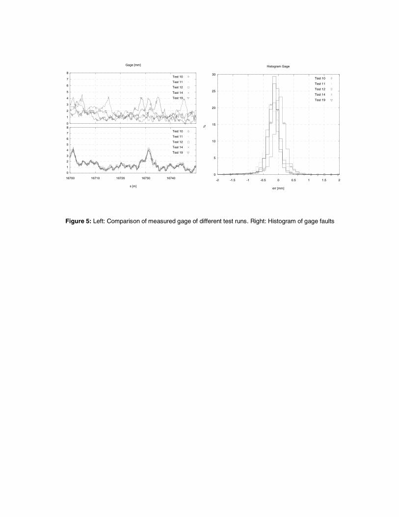
To synchronize the individual test channels we used an arbitrary data record as a reference. We then

grouped the other signals in 50 meter sections and shifted them against the reference data to achieve maximum

co-variance. The co-variance of two test values describes a match in signal form: the value 1 signifies identical

data, 0 stands for uncorrelative. Possible differences in the null balance do not influence this test. By shifting the

sections, a maximum correspondence of signals is guaranteed. The individual sections are shifted by a whole-

numbered multiple of the scanning rate (0.25 m) (see Figure 5, left).

The test values "optimally" synchronized by this method are separately averaged at each point. This

mean value is an approximation of the real test value. Thus, the differences between test runs and the common

test value are considered to be faults. Using common statistical methods, these faults are presented in a

histogram. Thus we get a stepped fault curve, which does not necessarily show a Gauss distribution. To be able

to judge the precision of this test system, all test faults are counted below a given limit and the defect is given in

per cent. The results of our analyses are shown in Figure 5, right.

5 EQUIVALENT CONICITY

Rail vehicle performance and behavior does not only depend on the type and design of the vehicles used but also

and in particular on the quality of the permanent way. Constant monitoring of track geometry in view of ensuring

traveling comfort and safety is becoming an increasingly important task for railway administrations. There is

more then one answer to the question of how traveling performance is affected by track geometry (see [2] – [6]).

A comprehensive analysis calls for the performance of time-consuming simulations with suitable programs. As

the computational and data requirements are so high, we need to restrict our examinations to smaller sections.

For a systematic evaluation, it turned out useful to look at the simpler issue of the geometric relations of the

contact between wheel gage and track cross section.

The important bearing function is primarily determined by the form fit of the tread of wheel and track.

More than 100 years ago, Klingel [1] was the first to become aware of the fundamental influence of the tread on

the motion of the rolling wheelset. This purely geometrical point of view constitutes the first attempt at

examining an essential aspect of the behavior of railroad vehicles. The conical form of the wheel gage and the

rigid connection of the wheels by the axle shaft cause the wheelset to self-locate on the track. Comparing the

behavior of a wheelset with real gages on the one hand to a double cone on the other hand provides the

equivalent conicity as a measure.

Commissioned by the Austrian Federal Railways (OBB) the Bureau of Applied Mechanics and Mathe-

matics (BAMM) developed the computer program QuiCon (QUIck CONicity), which is able to solve this prob-

lem online even during the measurement. Thanks to a non-contact optical measuring system, the EM250 can

measure rail profiles even at high running speeds. The output of these measurements are individual points that

are plotted in a Cartesian coordinate system. In order to study the contact geometry it is necessary to convert the

individual points into a smoothed curve. A special smoothing algorithm provides also an adequately smooth

course of the tangent line and the curvature.

In offline mode QuiCon is able to evaluate up to 100 pairs of rail profiles per second on a usual personal

computer. Thus it is possible to analyze the quality of rail profiles of the entire network during the test runs.

Figure 6 illustrates the points of contact on rail profile when the wheel is laterally displaced by y. In a nonlinear

iteration the roll angle ϕ and the height of the wheelset must be calculated numerically. The displacement y

results in a difference of the rolling radii ∆R. Due to a purely kinematic movement the wheelset describes a sinus

motion on the track with amplitude â (see Figure 7). The wave length λ depends on the conicity γ of the wheels

which stimulates the frequency of the vehicle according to the running speed.

In the following calculation the measured data of rail profiles and their interaction with a standard

wheel profile (ORE S1002) were analyzed. The results of calculations are represented as a function of distance s

and the lateral displacement of the wheel y (see Figure 8). The right part illustrates the differences in the running

radii ∆R for various rail profiles. Without flanging, the difference between the running radii is proportional to

lateral displacement and independent of amplitude. When the flange strikes against the rail head the difference

between the running radii increases markedly. A more detailed examination in the area of small displacements,

however, indicates marked differences between individual measuring points due to the presence of discontinuous

contact points with respect to y.

In the event of a piece-by-piece continuous linear ∆R function, a closed solution is possible, otherwise

only in special cases. A linearization of the differential equation of pure rolling will lead to more or less large

errors. The influence of measuring errors and errors of numerical evaluation were studied intensively (see UIC

Leaflet 519 [9]).

The following studies deal with the influence of gage and especially the rail profile onto the equivalent

conicity. This is to serve as an evaluation criterion of the quality of the rail profile. The measurements used for

the following analysis were performed on two different rail types (UIC54 and S49). Figure 9, left, shows the

gage as a function of the track length. The right part of Figure 9 describes the correlation of the equivalent

conicity and the gage. The equivalent conicity of rail type UIC54 is nearly double as high as that of S49. In low

gages — values lower than 1,432 mm — the conicity is high and the evaluations spread markedly. For higher

values of the gage it is possible to distinguish between the rail types.

6 RESULTS OF THE AUSTRIAN-WIDE MEASUREMENT CAMPAIGN

Figure 8 shows the cumulative frequency per rail profile of 381,187 equivalent conicity calculations measured in

the range of 0 to 0.5 all over the Austrian network. It therefore contains gages which are distributed according to

Figure 4 as well as nearly new and very worn rail profiles. Conicities of UIC54E are generally slightly higher

than conicities of the S49 rail profile. A significantly lower percentage of UIC 60 rail profiles exceeds conicities

of 0.3 compared to other profiles. As it is no longer usual to use the 44 kg rail on the OBB network, too little

measurements exist for this rail profile to get an adequate statistical overview.

7 CONCLUSIONS

Based on the enormous data supplied by the track recording car and the findings obtained from simulations, it is

possible to gain further insight into the complex behavior of vehicles and track in a quality hitherto unknown in

daily practice and state-of-the-art technology. This approach enables us to better understand the correlation

between disturbance variables and responses to these variables.

REFERENCES

[1] Klingel: Über den Lauf der Eisenbahnwagen auf gerader Bahn. Organ für die Fortschritte des

Eisenbahnwesens in technischer Beziehung 4, 113–123 (1883). (In German).

[2] Hainitz, H., Presle, G., Mittermayr, P.: Die Daten des neuen Oberbaumesswagens der ÖBB und deren

Anwendung in numerischen Simulationsprogrammen. Mitteilungen des Institutes für Öffentlichen

Verkehr der Universität Innsbruck Heft 8 (1997), 123–128. (In German).

[3] Presle, G, Hanreich, W., Mittermayr, P.: The Austrian track testing and recording car EM250: A Source

for Wheel/rail interaction analysis. Transport Research Board (2000).

[4] Presle, G, Mittermayr, P.: Beurteilung der Zuverlässigkeit des Fahrwegs durch Messung und

Simulation. ZEV–Glasers Annalen 2/3 (2000), 216–222. (In German).

[5] Mittermayr, P.: Simulation des Rad-Schieneverhaltens. ÖIAV Tagung "Produktinnovation im Maschi-

nenwesen durch Simulation". Wien 10.–11. April 2000, pp. 207–213. (In German).

[6] Presle, G., Mittermayr, P.: Assessment of the Reliability of the Track by Measurement and Simulation

(in German). Österreichische verkehrswissenschaftliche Gesellschaft 46, ÖVG-Tagung, Salzburg, 26.-

28. September, 2000.

[7] Rießberger, K. : Gleisgeometrie und Wirtschaftlichkeit – oder – wie gut muss ein Gleis sein? ÖVG –

Tagung Fahrwegoptimierung der Eisenbahnen – Innovationen, Erfolge, Perspektiven. Graz, 16. – 18.

September 1997.

[8] UIC Leaflet 518: Testing and approval of railway vehicles from the point of view of their behaviour –

Safety – Track fatigue – Ride quality. International Union of Railways.

[9] UIC Leaflet 519: Method for determining the equivalent conicity. International Union of Railways.

(Draft)

FIGURE CAPTIONS

Figure 1: The Austrian track geometry measurement coach EM250

Figure 2: Flow of measured data

Figure 3: Distribution of the MDZ track quality indices measured by the EM250 on the OBB network

Figure 4: Distribution of gage measurements taken by the EM250 on the OBB network (21.981.956

records)

Figure 5: Left: Comparison of measured gage of different test runs. Right: Histogram of gage faults

Figure 6: Contact points at wheel and rail at lateral displacement y

Figure 7: Definition of equivalent conicity

Figure 8: Difference of rolling radii ∆R and equivalent conicity γe as function of the track length s

Figure 9: Influence of gage and rail profile (left: gage as a function of track length, right: equivalent

conicity as a function of gage)

Figure 10: Distribution of conicity measurements of taken by the EM250 on the OBB network (381 187

records)

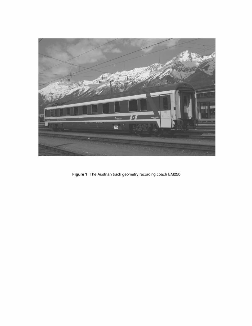
Figure 1: The Austrian track geometry recording coach EM250

onboard softwaredatawarehouse

small track

databease

upload+

check In

network topology

automaticgeneration small track

databease

upload+

check In

network topologynetwork topology

automaticgeneration

geometry datafiles (25cm)

TQI (500m)

permanentway

database

measurement runmeasurement run

user interface

TQI in theOBB Intranet

download ofgeometry datafiles

OffboardSoftware

databasequeries + statistics

Figure 2: Flow of measured data

0

1

2

3

4

5

6

7

8

9

10

0 -3 -6 -9 -12

-15

-18

-21

-24

-27

-30

-33

-36

-39

-42

-45

-48

Track Quality Index MDZ

freq

uen

cy d

istr

ibu

tio

n [

%]

0

10

20

30

40

50

60

70

80

90

100

cum

ula

tive

fre

qu

ency

[%

]

frequency distribution

cumulative frequency

Figure 3: Distribution of the MDZ track quality indices measured by the EM250 on the OBB network

0

5

10

15

20

25

30

35

40

45

50

40 to

38

36 to

34

32 to

30

28 to

26

24 to

22

20 to

18

16 to

14

12 to

10

8 to

64

to 2

0 to

-2

-4 to

-6

-8 to

-10

difference to nominal gage [mm]

freq

uen

cy d

istr

ibu

tio

n [

%]

0

10

20

30

40

50

60

70

80

90

100

cum

ula

tive

fre

qu

ency

[%

]

frequency distribution

cumulative frequency

Figure 4: Distribution of gage measurements taken by the EM250 on the OBB network (21.981.956 records)

0

1

2

3

4

5

6

7

8

16700 16710 16720 16730 16740

s [m]

Test 10

Test 11

Test 12

Test 14

Test 19

0

1

2

3

4

5

6

7

8

Gage [mm]

Test 10

Test 11

Test 12

Test 14

Test 19

0

5

10

15

20

25

30

-2 -1.5 -1 -0.5 0 0.5 1 1.5 2

%

err [mm]

Histogram Gage

Test 10

Test 11

Test 12

Test 14

Test 19

Figure 5: Left: Comparison of measured gage of different test runs. Right: Histogram of gage faults

y

r1 r2

∆R

ϕ

2r0

λ

γe

2â

y

x

Figure 6: Contact points at wheel and rail at lateral displacement y

Figure 7: Definition of equivalent conicity

Flangeway clearanceFlangeway clearance

Contact surface

28

21

14

7

0

-7

-14

-21

-28

28

21

14

7

0

-7

-14

-21

-28

1.20

1.05

.90

.75

.6

.45

.30

.15

0

1.20

1.05

.90

.75

.6

.45

.30

.15

0

ys âs

∆R[mm]

γe[ ]

Figure 8: Difference of rolling radii R and equivalent conicity γe as a function of the track length s

1425

1430

1435

1440

1445

1450

40000 45000 50000 55000

gage

[mm

]

s [m]

S49

UIC54

S49

0

0.2

0.4

0.6

0.8

1

1.2

1.4

1430 1432 1434 1436 1438 1440

ge

gage [mm]

S49 3mm

UIC54 3mm

UIC54

Figure 9: Influence of gage and rail profile (left: gage as a function of track length, right: equivalent conicity as a function of gage)

0

10

20

30

40

50

60

70

80

90

100

0 0,05 0,1 0,15 0,2 0,25 0,3 0,35 0,4 0,45 0,5

equivalent conicity for â=3mm

cum

ula

tive

dis

trib

utio

n p

er r

ail p

rofil

e [%

]

UIC 54E (144804 samples)

S 49 (122356 samples)

UIC 60 (110360 samples)

44kg (3667 samples)

Figure 10: Distribution of conicity measurements taken by the EM250 on the OBB network (381 187 records)