Traction Control of a Six-wheel Robot using Wheel Slip Dynamics

Viboon Sangveraphunsiri and Mongkol Thianwiboon

Robotics and Advanced Manufacturing Laboratory, Department of Mechanical Engineering Faculty of Engineering, Chulalongkorn University,

254 Phyathai Rd., Pathumwan, Bangkok, 10330, Thailand Tel. 66(2)218-6448, 66(2)218-6585, Fax. 66(2)218-6583

E-mail : viboon.s@eng.chula.ac.th, kieng@eng.chula.ac.th

Abstract

A method for kinematics modeling of a six-wheel Rocker-Bogie mobile robot is described in detail. The forward kinematics is derived by using wheel Jacobian matrices in conjunction with wheel-ground contact angle estimation. Te inverse kinematics is to obtain the wheel velocities and steering angles from the desired forward velocity and turning rate of the robot. Traction Control also developed to improve traction by comparing information from onboard sensors and wheel velocities to minimize slip of the wheel. Finally, a small robot is built and tested in various conditions of surfaces including vertical obstacle, inclined surface and uneven terrain outdoor condition.

Keywords: Rocker-Bogie Suspension / Traction Control / Slip Ratio 1. Introduction

The effectiveness of a wheeled mobile robot has been proven by NASA by sending a semi-autonomous rover “Sojourner” landed on Martian surface in 1997[1]. Future field mobile robots are expected to traverse much longer distance over more challenging terrain than Sojourner, and perform more difficult tasks. Other examples of rough terrain applications for robotic can be found in hazardous material handling applications, such as explosive ordnance disposal, search and rescue.

Corresponding to such growing attention, the researches are varying from mechanical design, performance of the robot, control system, navigation systems, path planning, field test, and so on.

However, there are very few dynamics of the robot. This is because the field robots are considered too slow to encounter dynamic effect. And the high mobility of the robot, moving in 3 dimensions with 6 degrees of freedom (X, Y, Z, pitch, yaw, roll), makes the kinematics modeling a challenging task than the robots which move on flat and smooth surface (3 degrees of freedom: X, Y, rotation about Z axis)

In rough terrain, it is critical for mobile robots to maintain maximum traction. Wheel slip could cause the robot to lose control and trapped. Traction control for low-speed mobile robots on flat terrain has been studied by Reister and Unseren [2] using pseudo velocity to synchronize the motion of the wheels during rotation about a point. Sreenivasan and Wilcox [3] have considered the effects of terrain on traction control by assume knowledge of terrain

geometry, soil characteristics and real-time measurements of wheel-ground contact forces. However, this information is usually unknown or difficult to obtain directly. Quasi-static force analysis and a fuzzy logic algorithm have been proposed for a rocker-bogie robot [4].

Knowledge of terrain geometry is critical to the traction control. A method for estimating wheel-ground contact angles using only simple on-board sensors has been proposed [5]. A model of load-traction factors and slip-based traction has been developed [6]. The traveling velocity of the robot is estimated by measure the PWM duty ratio driving the wheels. Angular velocities of the wheels are also measured then compare with estimated traveling velocity to estimate the slip and perform traction control loop.

In this research work, a small six-wheel robot with Rocker-Bogie suspension is designed, built and tested. The method to derive mathematical modeling such as, the wheel-ground contact angle estimation and kinematics modeling also described. Finally, a traction control system is developed and implemented on this robot.

2. Robot Test Bed In this research, the robot test bed named “Lonotech 10” is built. Its dimensions are 480x640x480 mm3, consists of six wheels, three on each side. Four steering mechanisms are equipped to the front and rear wheels.

Figure 1: Lonotech 10

All independently actuated wheels are connected by the Rocker-Bogie suspension, a

passive suspension that works well at low-velocity. This suspension consists of two rocker arms connected to the sides of the robot body. At one end of each rocker is connected to pivot of the smaller rocker, the bogie, and the other end has a steerable wheel attached. Two wheels are attached to the end of these bogies. The rockers connected to the body via a differential link. This configuration maintains the pitch of the body equal to the average angle between the two rockers. This mechanism also provides an important mobility characteristic of the robot: one wheel can be lifted vertically while other wheels remain in contact with the ground.

In order to climb over an obstacle, the front wheels are forced against the obstacle by the middle and rear wheels. Then the rotations of the front wheels lift the front of the robot up and climb over the obstacle. The middle wheels are pressed against the obstacle by the rear wheels and pulled by the fronts. Finally, the rear wheels are pulled by the front and middle wheels.

The robot equipped with various sensors for navigation. Most of the sensors are mounted on the pan-tilt mechanism, including CCD Camera, laser pointer, and distance measuring sensor. Three encoders are attached to the suspension to sense rocker and bogie angles. Inclinometers and accelerometer are also installed. The accelerometer is used to calculate the acceleration and velocity of the robot as the feedback data of the control system.

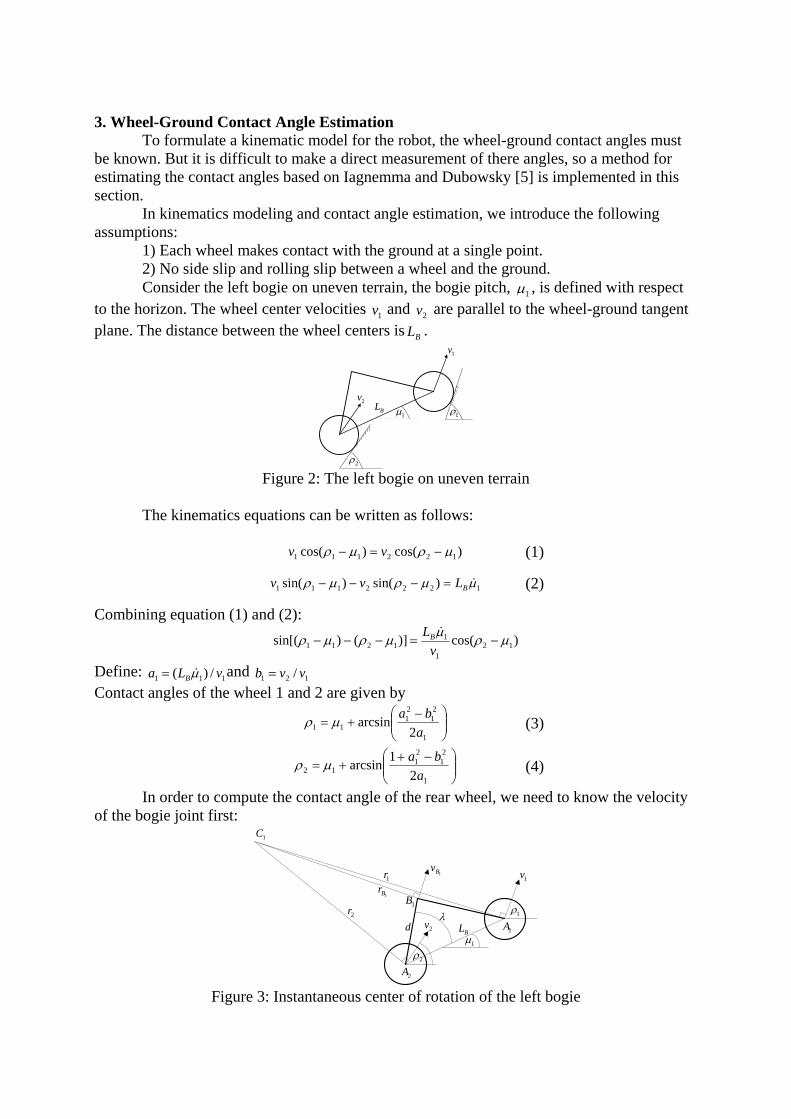
3. Wheel-Ground Contact Angle Estimation To formulate a kinematic model for the robot, the wheel-ground contact angles must be known. But it is difficult to make a direct measurement of there angles, so a method for estimating the contact angles based on Iagnemma and Dubowsky [5] is implemented in this section. In kinematics modeling and contact angle estimation, we introduce the following assumptions: 1) Each wheel makes contact with the ground at a single point. 2) No side slip and rolling slip between a wheel and the ground. Consider the left bogie on uneven terrain, the bogie pitch, 1μ , is defined with respect to the horizon. The wheel center velocities 1v and 2v are parallel to the wheel-ground tangent plane. The distance between the wheel centers is BL .

BL1μ 1ρ

2ρ

1v

2v

Figure 2: The left bogie on uneven terrain

The kinematics equations can be written as follows:

)cos()cos( 122111 μρμρ −=− vv (1)

1222111 )sin()sin( μμρμρ BLvv =−−− (2)

Combining equation (1) and (2): )cos()]()sin[( 12

1

11211 μρμμρμρ −=−−−

vLB

Define: 111 /)( vLa Bμ= and 121 / vvb = Contact angles of the wheel 1 and 2 are given by

⎟⎟⎠

⎞⎜⎜⎝

⎛ −+=

1

21

21

11 2arcsin

abaμρ (3)

⎟⎟⎠

⎞⎜⎜⎝

⎛ −++=

1

21

21

12 21arcsin

abaμρ (4)

In order to compute the contact angle of the rear wheel, we need to know the velocity of the bogie joint first:

BL1μ

1ρ

2ρ

1v

2vλ

d

2A

1A

1Bv1r

1Br

2r1B

1C

Figure 3: Instantaneous center of rotation of the left bogie

Define

1Br : rotation radius of the left bogie 1μ : angular velocity of the left bogie The velocity of the bogie joint can be written as:

111μBB rv =

where )90cos(2 122

2221

λμρ −−+−+= drdrrB

)sin()90sin(

21

121 ρρ

μρ−

−+= BLr

)sin()90sin(

21

112 ρρ

μρ−

+−= BLr

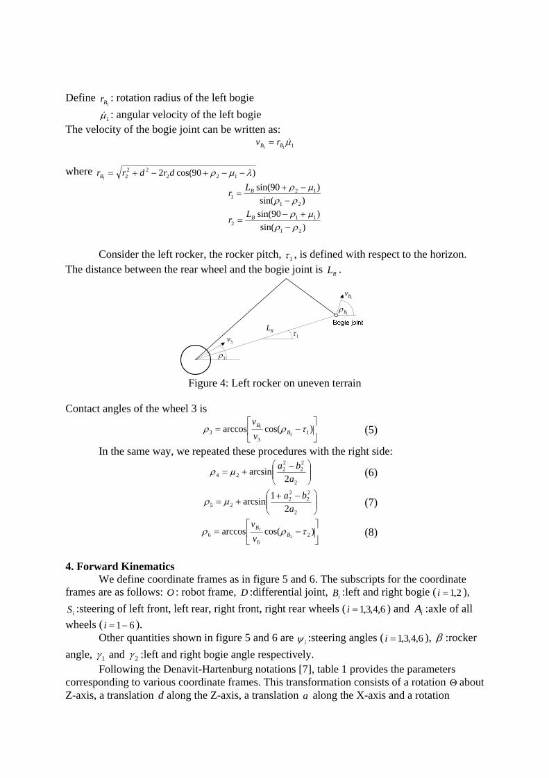
Consider the left rocker, the rocker pitch, 1τ , is defined with respect to the horizon. The distance between the rear wheel and the bogie joint is RL .

1Bv

RL1τ

1Bρ

3ρ

3v

Figure 4: Left rocker on uneven terrain

Contact angles of the wheel 3 is

⎥⎦

⎤⎢⎣

⎡−= )cos(arccos 1

33 3

1 τρρ BB

vv (5)

In the same way, we repeated these procedures with the right side:

⎟⎟⎠

⎞⎜⎜⎝

⎛ −+=

2

22

22

24 2arcsin

abaμρ (6)

⎟⎟⎠

⎞⎜⎜⎝

⎛ −++=

2

22

22

25 21arcsin

abaμρ (7)

⎥⎦

⎤⎢⎣

⎡−= )cos(arccos 2

66 2

2 τρρ BB

vv (8)

4. Forward Kinematics We define coordinate frames as in figure 5 and 6. The subscripts for the coordinate frames are as follows: O : robot frame, D :differential joint, iB :left and right bogie ( 2,1=i ),

iS :steering of left front, left rear, right front, right rear wheels ( 6,4,3,1=i ) and iA :axle of all wheels ( 61−=i ).

Other quantities shown in figure 5 and 6 are iψ :steering angles ( 6,4,3,1=i ), β :rocker angle, 1γ and 2γ :left and right bogie angle respectively.

Following the Denavit-Hartenburg notations [7], table 1 provides the parameters corresponding to various coordinate frames. This transformation consists of a rotation Θ about Z-axis, a translation d along the Z-axis, a translation a along the X-axis and a rotation

α about the X-axis. The transformation matrix for adjacent coordinate frame i to j can be written as follows:

⎥⎥⎥⎥

⎦

⎤

⎢⎢⎢⎢

⎣

⎡ΘΘ−ΘΘΘΘΘ−Θ

=

10000,

jjj

jjjjjjj

jjjjjjj

ij dCSSasCCCSCaSSCSC

αααααα

T

where jΘ , jα , ja and jd are the D-H parameters given for coordinate frame j . In this transformation, we have used the notation jCΘ = jΘcos and jSΘ = jΘsin , etc.

The transformations from the robot reference frame (O ) to the wheel axle frames ( iA ) are obtained by cascading the individual transformations. For example, the transformations for the wheel 1 are

111111 ,,,,, ASSBBDDOAO TTTTT =

OZ

DZDX

DY

OX OY

β2l

6l

8l3l

4l

5l

5l

537 lll +=

1SZ

1SX1SY

1ψ 3AZ

3AY

3AX

3ψ

1BX

1BY1BZ

1γ

1l

3SX3SY

1AZ

1AY

1AX

2AZ

2AY

2AX

3SZ

Figure 5: Left coordinate frames

DZ

DX

DYOX

OYβ−

2l

6l

8l

3l

4l

5l5l

537 lll +=

4SZ

4SX4SY

4AZ4AY

4AX

4ψ

5AZ5AY

5AX

6AZ

6AY

6AX

6ψ

2BY

2BZ 2γ2BX

1l

OZ6SZ

6SX

6SY

Figure 6: Right coordinate frame

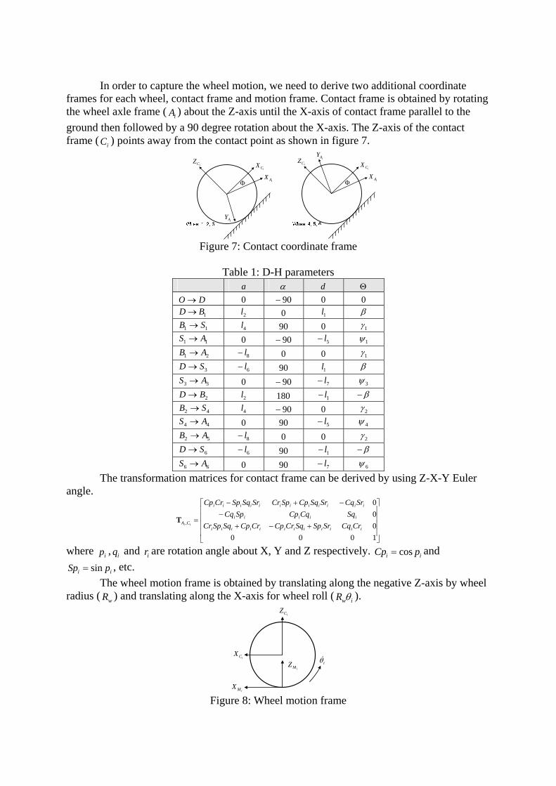
In order to capture the wheel motion, we need to derive two additional coordinate frames for each wheel, contact frame and motion frame. Contact frame is obtained by rotating the wheel axle frame ( iA ) about the Z-axis until the X-axis of contact frame parallel to the ground then followed by a 90 degree rotation about the X-axis. The Z-axis of the contact frame ( iC ) points away from the contact point as shown in figure 7.

iCXiCZ iAY

iAXΦ

iCXiCZ

iAY

iAXΦ

Figure 7: Contact coordinate frame

Table 1: D-H parameters

a α d Θ DO → 0 90− 0 0

1BD → 2l 0 1l β 11 SB → 4l 90 0 1γ 11 AS → 0 90− 5l− 1ψ 21 AB → 8l− 0 0 1γ

3SD → 6l− 90 1l β 33 AS → 0 90− 7l− 3ψ 2BD → 2l 180 1l− β− 42 SB → 4l 90− 0 2γ 44 AS → 0 90 5l− 4ψ 52 AB → 8l− 0 0 2γ

6SD → 6l− 90 1l− β− 66 AS → 0 90 7l− 6ψ

The transformation matrices for contact frame can be derived by using Z-X-Y Euler angle.

⎥⎥⎥⎥

⎦

⎤

⎢⎢⎢⎢

⎣

⎡

+−+−

−+−

=

1000000

,iiiiiiiiiiii

iiiii

iiiiiiiiiiii

CA CrCqSrSpSqCrCpCrCpSqSpCrSqCqCpSpCq

SrCqSrSqCpSpCrSrSqSpCrCp

iiT

where ip , iq and ir are rotation angle about X, Y and Z respectively. ii pCp cos= and

ii pSp sin= , etc. The wheel motion frame is obtained by translating along the negative Z-axis by wheel radius ( wR ) and translating along the X-axis for wheel roll ( iwR θ ).

iCZ

iCX

iMZ

iMX

iθ

Figure 8: Wheel motion frame

The transformation matrices for all wheels can be written as follows: 1111111111 ,,,,,,, MCCAASSBBDDOMO TTTTTTT =

22222112 ,,,,,, MCCAABBDDOMO TTTTTT =

33333333 ,,,,,, MCCAASSDDOMO TTTTTT =

4444444224 ,,,,,,, MCCAASSBBDDOMO TTTTTTT =

55555225 ,,,,,, MCCAABBDDOMO TTTTTT =

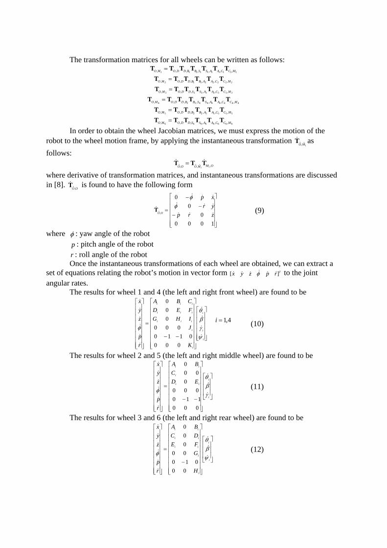
66666666 ,,,,,, MCCAASSDDOMO TTTTTT = In order to obtain the wheel Jacobian matrices, we must express the motion of the robot to the wheel motion frame, by applying the instantaneous transformation

iMO ˆ,ˆT as follows:

OMMOOO ii ,ˆ,ˆ,ˆ TTT = where derivative of transformation matrices, and instantaneous transformations are discussed in [8].

OO ,ˆT is found to have the following form

⎥⎥⎥⎥⎥

⎦

⎤

⎢⎢⎢⎢⎢

⎣

⎡

−−

−

=

10000

00

,ˆ zrpyrxp

OO

φφ

T (9)

where φ : yaw angle of the robot p : pitch angle of the robot r : roll angle of the robot Once the instantaneous transformations of each wheel are obtained, we can extract a set of equations relating the robot’s motion in vector form Trpzyx ][ φ to the joint angular rates. The results for wheel 1 and 4 (the left and right front wheel) are found to be

⎥⎥⎥⎥⎥

⎦

⎤

⎢⎢⎢⎢⎢

⎣

⎡

⎥⎥⎥⎥⎥⎥⎥⎥

⎦

⎤

⎢⎢⎢⎢⎢⎢⎢⎢

⎣

⎡

−−

=

⎥⎥⎥⎥⎥⎥⎥⎥

⎦

⎤

⎢⎢⎢⎢⎢⎢⎢⎢

⎣

⎡

i

i

i

i

i

iii

iii

iii

K

JIHGFEDCBA

rp

zyx

ψγβθ

φ

0000110

000000

4,1=i (10)

The results for wheel 2 and 5 (the left and right middle wheel) are found to be

⎥⎥⎥

⎦

⎤

⎢⎢⎢

⎣

⎡

⎥⎥⎥⎥⎥⎥⎥⎥

⎦

⎤

⎢⎢⎢⎢⎢⎢⎢⎢

⎣

⎡

−−

=

⎥⎥⎥⎥⎥⎥⎥⎥

⎦

⎤

⎢⎢⎢⎢⎢⎢⎢⎢

⎣

⎡

i

iii

i

ii

EDC

BA

rp

zyx

γβθ

φ

000110

0000

000

(11)

The results for wheel 3 and 6 (the left and right rear wheel) are found to be

⎥⎥⎥

⎦

⎤

⎢⎢⎢

⎣

⎡

⎥⎥⎥⎥⎥⎥⎥⎥

⎦

⎤

⎢⎢⎢⎢⎢⎢⎢⎢

⎣

⎡

−

=

⎥⎥⎥⎥⎥⎥⎥⎥

⎦

⎤

⎢⎢⎢⎢⎢⎢⎢⎢

⎣

⎡

i

i

i

i

ii

ii

ii

H

GFEDCBA

rp

zyx

ψβθ

φ

00010

00000

(12)

where θ is the angular velocity of the wheel, β is the rocker pitch rate, γ is the bogie pitch rate and ψ is the steering rate of the steerable wheel.

The parameter iA and iK in the matrices above can be easily derived in terms of wheel-ground contact angle ( 61..ρρ ) and joint angle ( γβ , and ψ ). For example, the parameter

1A of the front left wheel is

)()([))2(2(

111112

11 ψψργβ

ρSCCC

SA −+

+−= )]200400200( 1

21

21111 ρρρρψρ SCSCSS +−+

It is seen that these set of equations are in the general form iiqJu = 61−=i (13)

where iJ is the Jacobian matrix of wheel i , and iq is the joint angular rate vector. We will see that the 5th equation (5th row) does not contribute to any unknowns. It

simply states that the change in pitch is equal to the change in the bogie and rocker angles. With the help of an installed inclinometer, p can be sensed without knowledge of the rocker and bogie angles. Since only the p , in equation (10) to (12), contains γ and β , we can eliminate them from further consideration.

5. Inverse Kinematics The purpose of inverse kinematics is to determine the individual wheel rolling velocities which will accomplish desired robot motion. The desired robot motion is given by forward velocity and turning rate. In this section, we will develop all 6 wheels rolling velocities with geometric approach to determine steering angle of steerable wheels. 5.1 Wheel Rolling Velocities Consider the forward kinematics of the front wheel (10). Define the desired forward velocity as dx and desired heading angular rate as dφ . From equation (10), the first and the fourth equation give

iid

iiiiiid

J

CBAx

ψφ

ψγθ

=

++= 3,1=i (14)

The rolling velocities of the front wheels can be written as

i

di

iiid

i AJCBx φγ

θ−−

= 3,1=i (15)

Similarly, the rolling velocities of the middle wheels can be written as

i

iidi A

Bx γθ −= 5,2=i (16)

Finally the rolling velocities of the rear wheels can be written as

i

di

id

i AGBx φ

θ−

= 6,3=i (17)

5.2 Steering Angles Center of rotation, called turning center, is estimated based on the two non-steerable middle wheels. This turning center will be used to determine the steering angles of the four corner wheels. From figure 5 and 6, we can derive coordinate of the wheel centers respect to the robot reference frame as follows:

)sin()cos(sincos 1514321 γβγβββ −+−++= llllxC )sin()cos(sincos 1518322 γβγβββ −+−−+= llllxC

ββ sin)(cos 5363 lllxC ++−=

)sin()cos()sin()cos( 2524324 γβγβββ +−++−+−−−= llllxC )sin()cos()sin()cos( 2828325 γβγβββ +−++−−−−−= llllxC

ββ sin)()cos( 5366 lllxC +−−−=

x

z

Estimated InstantaneousCenter of Rotation

R

Figure 9: Instantaneous center of rotation

From figure 9, the instantaneous center of rotation can be estimated by averaging the x position of the middle wheels. The distance in Z-axis is neglected because there is only 1 degree of freedom per each steering. If the wheel’s axis is steered to intersect with the center of rotation on the X-axis, the angle in Z direction is coupled and cannot be controlled. Using the estimated center of rotation, the desired steering angle for each steerable wheel can be determined. Define R is a turning radius, Rx is the distance in X-direction of the center of rotation with respect to the robot reference frame, 1l is the distance from the robot reference frame to steering joint in Y-direction (see figure 5 and 6). The desire steering angles are

⎟⎟⎠

⎞⎜⎜⎝

⎛−−

=1

11 arctan

lRxx RCψ for wheel 1

⎟⎟⎠

⎞⎜⎜⎝

⎛−−

=1

33 arctan

lRxx RCψ for wheel 3

⎟⎟⎠

⎞⎜⎜⎝

⎛−−

=1

44 arctan

lRxx RCψ for wheel 4

⎟⎟⎠

⎞⎜⎜⎝

⎛−−

=1

66 arctan

lRxx RCψ for wheel 6

6. Motion Control 6.1 Wheel Slip Dynamics Consider the model consists of a single wheel supported a mass m . As the wheel rotates, driven the mass m in the direction of the velocity v . A torque applied to the wheel cause the angular velocity ω . A reaction force xF is generated by the friction between wheel and ground. The equations of motion of single wheel can be written as

xF

zF

ω

τ

v

Figure10: Forces and torques on a wheel

xFvm = (18)

xrFJ −=τω (19)The friction force xF is given by

),,( αμμ Hzx SFF = (20)where zF is the vertical force, the friction coefficient μ is a nonlinear function of the maximum friction between wheel and ground ( Hμ ) and the slip angle of the wheel (α ). The slip ratio S , describes the normalized difference between traveling velocity of the wheel and the wheel circumference velocity, is defined as follows (Yoshida and Hamano [6]):

⎩⎨⎧

<−>−

=):(/)():(/)(

ngdecelerativrvvrngaccelerativrrvr

Sωωωωω

For example, in the latter case, we get

Jr

vSF

JrS

mvS HZ

ταμμ 1),,()1(11 2

+⎟⎟⎠

⎞⎜⎜⎝

⎛++−= (21)

6.2 Traction Control In section 4 and 5, we assume that there is no side slip and rolling slip between wheel and ground. Then slip must be minimizing to guarantee accuracy of the kinematics model.

The control problem is to control the slip S to a desired set point *S that is either constant or commanded from a higher-level control system. The feedback value is computed from a slip estimator. To complete the estimation of the slip, we need the rolling velocity and the traveling velocity of the wheels, ω and v . Rolling velocity of the wheel is easily obtained from encoders which installed in all wheels. Traveling velocity of the wheel can compute from robot velocity by using data from onboard accelerometer. The robot velocity can be obtained by integrating the accelerometer signal. Then use this value as an input for the inverse kinematics (equation 15-17) to compute the rolling velocities of the wheels. Then multiply these rolling velocities by wheel radius, we can obtain the traveling velocity of the wheels. Integral adaptation must be incorporated to remove steady-state error due to model inaccuracies, in particular the unknown wheel-ground friction coefficient Hμ

For the controller design, we consider (21) and linearized the model, let )ˆ,ˆ( τS be an equilibrium point for (21) defined by the nominal values α̂ , ZF̂ and Hμ̂ then

)ˆ,ˆ,ˆ(ˆ)ˆ1(ˆ αμμτ HZ SFrSmrJ

⎥⎦⎤

⎢⎣⎡ ++=

The speed-dependent nominal linearized slip dynamic is ...)ˆ()ˆ( 11 toh

vSS

vS +−+−= ττβα (22)

where 1α and 1β are linearization constants:

)ˆ,ˆ,ˆ()ˆ1(1ˆ2

1 αμμα HZ SSJ

rSm

F∂∂

⎥⎦

⎤⎢⎣

⎡++−= )ˆ,ˆ,ˆ(ˆ1 αμμ HZ SF

m−

Jr /1 =β Define *

2 SSx −= , and assuming arbitrary values of ZF,α and Hμ , the wheel slip dynamics (21) can be written as

Traction Control

Desired Robot Motion

Cartesian SpacePID Controller

Floor to RobotVelocity

Transformation

Steering AngleEstimation Steering Control

InverseKinematics

Wheel MotionControl

+

-

+

-

Sensed Wheel Rolling Velocity

Sensed Robot VelocityInverseKinematics

+

-

-

ForwardKinematics

Sensed Wheel Rolling VelocityRobot to FloorVelocity

Transformation

Dead ReckoningIntegration

+

-

Slip estimator

Actual Wheel Velocity

Desired Slip Ratio

Figure 11: Robot control schematic

)()( *12

2 ττβφ−+=

vvxx (23)

where

),,()1(1)( *2

2

2*

2 αμμφ HZ SxFJrxS

mx +⎥

⎦

⎤⎢⎣

⎡+++−= ),,()1( *** αμμτ HZ SFrS

mrJ

⎥⎦⎤

⎢⎣⎡ ++=

It can be seen that (23) has an equilibrium point given by *2 ,0 ττ ==x since 0)0( =φ , and the

linearized slip model (22) with a perturbation term written as

vx

vx

vx

)()( 2*1

21

2μεττβα

+−+= (24)

where 2122 )()( xxx αφεμ −= Let the system dynamics (24) be augmented with a slip error integrator 2

*1 xSSx =−=

)()())(()( 2*

2

1

2

1 xvWuvBxx

vAxx

μετ +−+⎭⎬⎫

⎩⎨⎧

=⎭⎬⎫

⎩⎨⎧

where

⎥⎥⎦

⎤

⎢⎢⎣

⎡=

vvA 10

10)( α ,

⎪⎭

⎪⎬⎫

⎪⎩

⎪⎨⎧

=v

vB 1

0)( β ,

⎪⎭

⎪⎬⎫

⎪⎩

⎪⎨⎧

=v

vW 10

)(

The steady-state torque *τ depends on wheel and ground properties such as Hμ and must therefore be assumed unknown. So we define the control input τ=u , and the equilibrium point is

⎭⎬⎫

⎩⎨⎧

=0

*1* x

x , ** τ=u

where *1x depends on the controller. This leads to

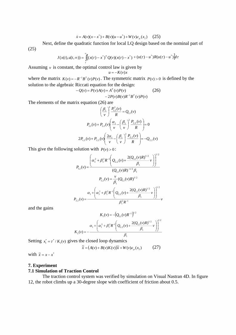
)()())(())(( 2** xvWuuvBxxvAx με+−+−= (25)

Next, define the quadratic function for local LQ design based on the nominal part of (25)

[∫∞

−−=∞t

T xxvQxxtutxJ ))()(())(()),[),(( ** ττ ] τττ duuRuu ))(())(( ** −−+

Assuming v is constant, the optimal control law is given by xvKu )(−=

where the matrix )()()( 1 vPvBRvK T−−= . The symmetric matrix 0)( >vP is defined by the solution to the algebraic Riccati equation for the design:

)()()()()( vPvAvAvPvQ T+=− )()()()(2 1 vPvBRvBvP T−−

(26)

The elements of the matrix equation (26) are

)()(

1,1

22,1

21 vQ

RvP

v=⎟

⎠⎞

⎜⎝⎛ β

0)(

)()( 2,22

112,11,1 =⎟

⎟⎠

⎞⎜⎜⎝

⎛⎟⎠⎞

⎜⎝⎛−+

RvP

vvvPvP βα

)()(2)()(2 2,2

2,22

112,22,1 vQ

RvP

vvvPvP −=⎟

⎟⎠

⎞⎜⎜⎝

⎛⎟⎠⎞

⎜⎝⎛−+βα

This give the following solution with 0)( >vP :

12/1

1,1

2/1

1

2/11,1

2,212

121

1,1 ))((

))((2)(

)(β

ββα

−

−

⎟⎟⎠

⎞⎜⎜⎝

⎛⎟⎟⎠

⎞⎜⎜⎝

⎛++

=RvQ

vRvQ

vQR

vP

2/11,1

12,1 ))(()( RvQvvP

β=

vR

vRvQ

vQR

vP 121

2/1

1

2/11,1

2,212

1211

2,2

))((2)(

)( −

−

⎟⎟⎠

⎞⎜⎜⎝

⎛⎟⎟⎠

⎞⎜⎜⎝

⎛+++

=β

ββαα

and the gains ( ) 2/11

1,11 )()( −−= RvQvK

1

2/1

1

2/11,1

2,212

1211

2

))((2)(

)(β

ββαα ⎟

⎟⎠

⎞⎜⎜⎝

⎛⎟⎟⎠

⎞⎜⎜⎝

⎛+++

−=

− vRvQ

vQR

vK

Setting )(/ 1**

1 vKx τ= gives the closed loop dynamics ( ) )()(~)()()(~

2xvWxvKvBvAx με++= (27) with *~ xxx −= 7. Experiment 7.1 Simulation of Traction Control The traction control system was verified by simulation on Visual Nastran 4D. In figure 12, the robot climbs up a 30-degree slope with coefficient of friction about 0.5.

Figure 12: Robot climbing up a slope

As a result, in the case without control, the robot was running at 55mm/s, and then the

front wheels touched the slope at 5.0=t sec. and begin to climb up. Robot velocity reduced to 25mm/s. But the robot can continue to climb until the middle wheels touch the slope at

9=t sec. as shown in the figure 14. The velocity decreased to nearly zero. In case with control, the sequence was almost the same until 5.0=t sec. The velocity reduced to approximately 35mm/s when the front wheels touched the slope. At 6=t sec., the middle wheel touched the slope and velocity reduced to 28 mm/s. And both rear wheels begin to climb up the slope at 15=t sec. with velocity approximately 20mm/s. In figure 13, the robot traversed over a ditch, which has 32mm depth and 73mm width with coefficient of friction about 0.5.

Figure 13: Traversing over a ditch

-15

-5

5

15

25

35

45

55

0 2 4 6 8 10 12 14 16

time (s)

Rob

ot V

eloc

ity (m

m/s

)

w/o traction controltraction control

-0.2

0

0.2

0.4

0.6

0.8

1

1.2

0 2 4 6 8 10 12 14 16

time (s)

Slip

Rat

io

w/o traction controltraction control

Figure 14: Velocity and slip ratio when climbing a 30 degree slope

-50

0

50

100

150

200

0 2 4 6 8 10 12 14 16

time (s)

Robo

t Vel

ocity

(mm

/s)

w/o traction controltraction control

-1

-0.5

0

0.5

1

1.5

0 2 4 6 8 10 12 14 16

time (s)

Slip

Rat

io

w/o traction controltraction control

Figure 15: Velocity and slip ratio when traversed over a ditch

The robot was commanded to move at 55mm/s, and then the front wheels went down the ditch at 5.0=t sec. The velocity of the robot increased temporary and begin to climb up when fronts wheels touch the up-edge of the ditch. But the wheels slipped with the ground and failed to climb up. Then the slip ratio went up to 1 ( 1=S ), the robot has stuck and the velocity decreased about zero at 5.1=t sec. With traction control, after the front wheels went down the ditch, the slip ratio was increased. Then the controller tried to decelerate to decrease the slip ratio. When the slip ratio was around 0.5, the robot continued to climb up. Until 5.4=t sec., both of the front wheels went up the ditch completely and the robot velocity increased to 55mm/s as commanded.

At 6=t sec., the middle wheels went down the ditch. The velocity also increased temporary and back to 55mm/s again when the middle wheels went up completely. The last two wheels went down the ditch at 13=t sec. and the sequence was repeated in the same way as front and middle wheels.

bogie

rocker

Figure 16: Step climbing situation

When the front wheel climbed up a step, the bogie pivot retreated and pushes the rear

wheel backward resulting in rear wheel slippage. This problem can be improved by lowering the bogie pivot below the front wheel axis.

Figure 17: Lowering the bogie pivot

Another way to reduce this problem is performing wheelie maneuvers. This method

varies the speed of the wheels to articulate the frame, allow the wheels to move closer or further apart. The wheelie maneuvers divided into two stages. First, when the obstacle approaches, speed up the middle wheels and slow down the rear wheels to lift the front wheels. When the front wheels are over the obstacle, return all wheels to normal speed. The second stage is to lift the middle wheels over the obstacle. This can be done by slow down the front wheels and speed up the rear wheels. Then return to normal speed again when the obstacle is under the middle wheels. The rear wheels cannot lift up by this method due to limitation of the rocker-bogie configuration. 7.2 Field Test The robot was tested outdoors with various surface conditions, such as climbing over a curb, climbing up a slope, and traversing over obstacles scattered on the ground. The robot was commanded to move at 50mm/s and able to climb up a curb of height 100mm, perpendicular to the movement.

Figure 18: Climbing up a curb

Climbing up an inclined surface was also tested. The slope was 40 degrees. The robot can climb the slope easily. Furthermore, it can stop and change direction on the slope.

Figure 19: Climbing up a slope

Figure 20: Traversing over obstacles

In the experiment, the robot can climb up a steeper slope than in the simulation. This because the coefficient of friction between wheel and ground in the real world is much higher than in simulation and the rolling slip model is excluded in the simulation. The geometry of the wheel surface also affects climbing ability. 8. Conclusion In this paper, wheel-ground contact angle estimation has been presented and integrated into a kinematic model. Unlike available methods applicable to robots operating on flat and smooth terrain, the proposed method uses the Denavit-Hartenburg notation like a serial link robot, due to the rocker-bogie suspension characteristics. The steering angle is estimated with a geometric approach.

A traction controller is proposed based on estimation of the slip ratio. The slip ratio is estimated from wheel rolling velocities and the robot velocity. The traction control strategy is to minimize this slip ratio. So the robot can traverse over obstacle without being stuck.

The traction control strategy is verified in the simulation with two conditions: climbing up the slope and moving over a ditch. Then the control system is implemented in a robot test bed “Lonotech 10” and tested in the real world, outdoor condition to verify the simulation results. 9. References [1] JPL Mars Pathfinder. February 2003. Available from: http://mars.jpl.nasa.gov/MPF [2] D.B.Reister, M.A.Unseren, “Position and Constraint force Control of a Vehicle with Two or More Steerable Drive Wheels”, IEEE Transaction on Robotics and Automation, page 723-731, Volume 9, Dec 1993. [3] S.Sreenivasan, B.Wilcox, “Stability and Traction control of an Actively Actuated Micro Rover”, Journal of Robotic Systems, 1994. [4] H.Hacot, “Analysis and Traction Control of a Rocker-Bogie Planetary Rover”, M.S.Thesis, Massachusetts Institute of Technology, Cambridge, MA, 1998. [5] K.Iagnemma, S.Dubowsky, “Mobile Robot Rough-Terrain Control (RTC) for Planetary Exploration”, Proceedings of the 26th ASME Biennial Mechanisms and Robotics Conference, Sep.10-13, 2000, Baltimore, Maryland. [6] K.Yoshida, H.Hamano, “Motion Dynamics of a Rover with Slip-Based Traction Model”, Proceeding of 2002 IEEE International Conference on Robotics and Automation, 2002. [7] John J. Craig, “Introduction to Robotics Mechanics and Control”, Second Edition, Addison-Wesley Publishing, 1989. [8] Patrick F. Muir, Charles P. Neumann, “Kinematic modeling of wheeled mobile robots”, Journal of Robotics Systems, Vol.4, No.2, pp.281-340, 1987.