trade patterns, trade balances and idiosyncratic shocks - caixabank research · 2019-03-05 ·...

The views expressed in this working paper are those of the authors only and do not necessarily represent those of “la Caixa”

Trade Patterns, Trade Balances and Idiosyncratic Shocks C. Canals, X. Gabaix, J. Vilarrubia, D.E. Weinstein June 2007

Working Paper Series No. 02/2007

Research Department Av. Diagonal, 629 T.I P.6 08028 Barcelona - Spain [email protected]

Trade Patterns, Trade Balances and Idiosyncratic

Shocks

Claudia Canals �, Xavier Gabaixy, Josep M Vilarrubiaz, David Weinsteinx

First Draft: May 2005 This Draft: June 2007

Abstract

International Macroeconomics has long sought an explanation for currentaccount �uctuations that matches the data. The approaches have typicallyfocused on better models and new macroeconomic variables. We demonstratethe limitations of this approach by showing that idiosyncratic shocks are animportant cause of macroeconomic volatility even for large countries. Whenexplaining these �uctuations, standard macroeconomic models generally as-sume that �rms are small and that their microeconomic shocks cancel out. Weshow that the high degree of concentration of bilateral trade �ows means thatidiosyncratic shocks can have a signi�cant impact on aggregate economic �uc-tuations. We theoretically develop a decomposition of the variance of trade�ows into its macroeconomic and its microeconomic components. Taking themodel to data on bilateral trade �ows from 1970 to 1997, we �nd that themost comprehensive macroeconomic model can only account for at most halfof the observed variance in trade account volumes of each country. Thus,this paper highlights the importance of considering disaggregated data whenmodeling the current account.

c Caja de Ahorros y Pensiones de Barcelona, "la Caixa"c C. Canals, X. Gabaix, J. Vilarrubia, D. Weinstein

�"la Caixa" Av Diagonal 629, T.1 P.6 08028 Barcelona - Spain. email: [email protected]: http://www.claudiacanals.com

yMIT and NBER. MIT Department of Economics E52-274b 50 Memorial Drive Cambridge MA02142-1347, US. email: [email protected]

zBanco de España. email:[email protected] University and NBER. Economics Department. Columbia University. 420 W 118th

Street MC 3308 New York, NY 10027, US. email: [email protected]

1

Trade Patterns, Trade Balances and Idiosyncratic Shocks

1 Introduction

There is a deep disconnect between the types of variables that economists typically

turn to when explaining trade balance �uctuations and those used by market an-

alysts. Consider, for example, a typical news story discussing the release of trade

de�cit numbers drawn from The New York Times:

�America�s appetite for foreign imports broke all records in January, reaching $159.1 billion

and contributing to a monthly trade de�cit that is the second highest on record. The $58.3 billion

trade de�cit de�ed predictions that a weakened dollar and lower oil prices would narrow the United

States�trade gap.

Instead, the Commerce Department said on Friday that American consumers continued to

buy foreign-made goods at an avid pace, raising the trade de�cit 4.5 percent from $55.7 billion

in December. January�s trade �gures included a 75 percent surge in Chinese textile and apparel

shipments, re�ecting the end to global quotas and the beginning of what some experts see as a

future of China supplying as much as 70 percent of the United States textile and apparel market.�-

Elizabeth Becker, �Trade Gap Widens on Record Imports,�The New York Times, March 11, 2005,

p. C1.

As the quotation makes clear, economic forecasters tend to focus on macroeconomic

variables � exchange rates, oil prices, etc. �while market analysts often turn to

more idiosyncratic explanations of trade balance movements, in the example above

Chinese textile shipments.

This paper seeks to understand the relative importance of macroeconomic and idio-

syncratic shocks in trade balance movements. We de�ne �macroeconomic shocks�

as movements in the trade balance that can be attributed to characteristics of the

importer, the exporter or the industry and �idiosyncratic shocks� as those which

are speci�c to each individual trade �ow. We �nd that each kind of shock can

explain around one half of the total variance of the trade balance for the typical

OECD country. This suggests that the di¢ culty economists have had in explaining

trade balance �uctuations may not be due to using the wrong set of macroeconomic

variables or the wrong models. Instead, we document that economies are bu¤eted

by large idiosyncratic shocks that do not �t easily into a standard macroeconomic

framework. We identify an idiosyncratic shock as one a¤ecting a particular trade

�ow with respect to a given location in a given industry. For example, a surge in oil

Canals, Gabaix, Vilarrubia, Weinstein 2 "la Caixa" WPS No 02/2007


prices could push up demand for fuel-e¢ cient cars in the United States which could,

in turn, lead to an increase in Japanese car exports to the United States without

directly a¤ecting the rest of Japanese exports (in other industries) or exports of

Japanese cars to other destinations.

On some level, the distinction between idiosyncratic shocks and macroeconomic

shocks is semantic. Macroeconomic identities must hold, and since all trade bal-

ance movements can be decomposed into demand and supply shocks, one could

argue that all shocks to the trade balance must, by de�nition, be macroeconomic.

Seen in this context, our de�nition of �macroeconomic shock� is closer to �com-

mon shock.� That said, there is a good reason for using the term �macroeconomic

shock.�Macroeconomic models and empirical exercises focus almost exclusively on

country- or industry-level variables such as GDP �uctuations or movements in the

price of oil and other commodities. As a result, while it is fair to say that most

macroeconomists already know that country-industry shocks could matter, it is also

fair to say that these have largely been ignored.

There are several reasons why economic explanations for trade balance and current

account movements have focused on common rather than idiosyncratic shocks. First,

these are, by far, the easiest forces to model. Idiosyncratic shocks are necessarily

messy and do not lend themselves easily to beautiful theory. Secondly, most inter-

national macroeconomic models tended to assume that demand is homothetic and

output is specialized. These two assumptions work together to guarantee that im-

port volumes are not highly concentrated in particular country-industry �ows. If all

bilateral trade �ows are small, the Law of Large Numbers applies, and idiosyncratic

shocks will not have much of an impact on aggregate trade �ows. Unfortunately,

these assumptions do not seem to hold in the data where the top 1% of largest �ows

account for 75% of total US exports, meaning that 99% of �ows account for only

25%. This implies that idiosyncratic shocks could aggregate to non-trivial shocks.

While there is no question that both forces - common and idiosyncratic - are impor-

tant in determining the level of national net exports, economic theory has almost

entirely focused on the former determinants of trade balances. In this paper, we

argue that ignoring the latter is not an innocuous assumption.

This paper develops a theoretical model that is taken to the data on bilateral trade

�ows in order to quantify the importance of these country-industry shocks. Our

empirical speci�cation corresponds to the best conceivable macroeconomic model of



the global economy, one that would perfectly forecast the typical behavior of every

industry and every country. Our measure of idiosyncratic shocks, then, stems from

shocks to particular country-industry pairs. We �nd that the idiosyncratic shocks in

our model could account for up to 24% of the behavior of exports and up to 31% for

imports in the typical OECD country. Unfortunately, common shocks do not fare

so well at explaining the evolution of trade balances where they can only account

for up to 45% of the total variation, leaving the remaining 55% to be explained

by idiosyncratic shocks. This implies that every three years, one sees movements

in exports of almost 50% of the actual growth rate due to idiosyncratic shocks.

Similarly, the corresponding movements in import and trade balance growth are

around 65% and 110%, respectively.

The magnitude of these numbers suggests that there is room for both macroecono-

mists and analysts when making predictions of the trade account since both common

and idiosyncratic shocks seem to be important at moving aggregate �ows.

This paper is organized as follows. Section 2 contains a literature review, while the

motivation for our study showing the lumpiness and the volatility of trade �ows is

given in section 3. A basic theoretical model is introduced in section 4 and taken

to the data in section 5. Section 6 shows the results of the empirical estimation.

Section 7 presents a particular study of what could be driving idiosyncratic shocks

using Japan as an example. Finally, section 8 concludes.

2 Literature survey

Our paper connects to several lines of enquiry. In the last few years, a large and

increasing body of literature has focused on the importance that heterogeneous �rms

could have in explaining several features of international trade �ows (Bernard et al.

2003, Chaney 2005, Eaton, Kortum and Kramarz 2005, Melitz 2002) or industries

(Alvarez and Lucas 2005, Eaton and Kortum 2002). The main motivation for this

work is that the ultimate determinant of trade �ows will be better understood by

looking at the microeconomic data. Tipically, those models are static and, in their

simplest dynamic extension, they would predict that, for instance, a productivity

shock in a given country would cause exports to increase by the same proportion

across all destination countries. Our �ndings lead to an even more disaggregated

view. For example, a given shock to Toyota will typically have very varied outcomes



across destination countries. We suspect that this has to do with other additional

factors generally unknown to the observer such as �t of the given product to the

country, the existence of distribution networks, or the intensity of the local compe-

tition. Establishing the main reasons for the idiosyncratic impact of shocks remains

an open research question.

We also suspect that analysis of trade shocks may shed light on the perennial ques-

tion of the determinants of trade. Interestingly, most models (e.g. the monopolistic

competition model in Helpman and Krugman 1985) would typically predict a fairly

homogenous structure of trade across destination countries, which in its pure form

is at odds with the data (Davis and Weinstein 2001, 2002).

Our paper may also help �esh out the shocks postulated in models of the current

account (Obstfeld and Rogo¤ 1996, Backus, Kehoe and Kydland 1992, Kray and

Ventura 2003). These models typically postulate an aggregate demand or supply

shocks per period. Again, our results may inform future developments in model of

the current account.

Finally, our paper relates to work that focuses in those instances where a few large

idiosyncratic agents could a¤ect aggregate outcomes. Gabaix et al. 2003 explores

this e¤ect for the stock market while, Gabaix 2005 theoretically and empirically

studies this hypothesis for the aggregate macroeconomy. He shows how, if �rm

sizes are distributed according to a fat-tailed distribution (a plausible assumption

when one analyzes the data), a few large �rms will account for a non-vanishing

fraction of the economic activity. Hence, implying that idiosyncratic �rm shocks

could potentially generate sizable aggregate �uctuations. In this paper, we explore

the existence of similar e¤ects in our trade �ow data.

3 Lumpiness and Idiosyncratic Volatility

In this section, we aim to demonstrate that bilateral trade �ows are not only lumpy

but also subject to idiosyncratic volatility. To this e¤ect, in the �rst subsection we

compute various concentration ratios and Her�ndahl indices to ascertain the degree

of lumpiness. In the next subsection, we report di¤erent measures of idiosyncratic

volatility of bilateral trade �ows.



3.1 Lumpiness

Simple inspection of the data on bilateral trade �ows reveals that these are, indeed,

very concentrated. This lumpiness becomes evident at three di¤erent levels. First,

looking at the industrial composition of a country�s total trade, we �nd that the

bilateral �ows of a few industries account for a large portion of overall trade. For

our sample of 24 OECD countries, the top 5 traded industries account for over 55%

of total exports and imports for the typical country1. This share of the top 5 traded

industries with respect to total exports and imports for each country is depicted in

Figure 1. Secondly, if we look at the destinations (origins) of a country�s exports

(imports), we �nd that a small number of countries account for a very large portion

of each country�s overall exports (imports). As shown in Figure 2, the top 5 trading

partners account for around 55% of total trade �ows for the typical country2.

Furthermore, �ows are not only concentrated at the country and at the industry

level but also at the country-industry level. In other words, a few trade �ows with

respect to a few countries in a few industries account for a large portion of overall

trade �ows. Figures 3 and 4 show the importance of the top 1% and 5% largest �ows

to total trade for exports and imports, respectively. The data for these �gures is

available in Table 1. Inspecting these data, it is apparent that only the top 1% trade

�ows account for over 80% of the total trade volume for the typical OECD country

(and over two thirds for any country). If we consider the top 5% trade �ows, these

cover over 92% of total exports and over 98% of total imports. Since each country

could potentially trade in 59 industries with 140 trading partners, keeping track

of the top 1% of �ows means considering at most 83 country-industry pairs which

would allow us to track the practical entirety of total exports or imports for any

given country3. To get a sense of concentration in terms of the number of �ows,

we compute the importance of the top 25 and 100 raw country-industry �ows for

exports and imports and we report them in Table 2. The largest 25 �ows account

for almost two thirds of total trade for the average country while the largest 100

�ows a country for over 85% of total trade.

Another commonly used measure of concentration is the Her�ndahl Index. Just like

with the concentration ratios above, we can compute this index at three separate

1Our data comprise 59 2-digit SITC industries.2We use data of bilateral trade �ows between 24 OECD countries with respect to 141 trading

partners.3For a potential maximum number of observations of (59 � 140 =) 8260.



levels: country, industry, and country-industry.

First, we calculate the Her�ndahl index for industry �ows which informs us about

the degree of industrial concentration in a country�s trade. We de�ne country c�s

industry Her�ndahl at time t as:

IHct =Xi

�2cit where �cit =

Pc0 Scc0itPc0i Scc0it

where Scc0it corresponds to the trade �ow between country c and c0 in industry i at

time t. We compute IHct for every country and year and report the yearly average

for each country in Table 3. Not surprisingly, there is a high degree of correlation

between these Her�ndahl indices and the concentration ratios obtained earlier. The

median industry Her�ndahl for our sample of 24 OECD countries is about 0.09 for

exports and 0.1 for imports both indicating a high degree of concentration at the

industry level4.

Analogously, we compute a Her�ndahl index for country �ows to get a sense of

the geographical concentration of a country�s trade. We de�ne country c�s country

Her�ndahl at time t as:

CHct =Xc0

�2cc0t where �cc0t =

Pi Scc0itPc0i Scc0it

Again, we compute CHct for every country and year and report the yearly average

for each country in Table 4. The median country Her�ndahl for our sample is about

0.11 for exports and 0.09 for imports5. It is particularly striking the high degree

of concentration of Canadian and Mexican trade (with the United States) which

results in a very high Her�ndahl index for these two countries.

Finally, we move our focus to country-industry �ows by computing what we call the

overall Her�ndahl. We de�ne country c�s overall Her�ndahl at time time t as:

OHct =Xc0i

�2cc0it where �cit =Scc0itPc0i Scc0it

4A low degree of concentration at the industry level would be if all 59 industries had the sameshare in the country. Thus, we would obtain an industry Her�ndhal of 0.016, which is �ve timessmaller that the one obtained.

5A low degree of concetration is found when we import or export to each country the sameamount. In this case the Her�dhal would be 0.07, again a lot lower that the one obtained



In this case, the higher degree of disaggregation6 means that the share of each �ow

(�cc0it) is smaller resulting in substantially lower Her�ndahls. The typical Her�ndahl

for country-industry �ows is about 0.03 for exports and 0.04 for imports which still

indicate a high degree of concentration.

3.2 Idiosyncratic Volatility

In order to show whether bilateral trade �ows are volatile, we start by constructing

a measure of idiosyncratic volatility at the industry level as follows. For a given

country and year, we compute the growth rate of exports (imports) for each industry,

from this number we subtract the growth rate of total exports (imports) in that

country in that given year and obtain what we call �demeaned growth rates�. These

growth rates give us an idea of the di¤erential behavior of exports (imports) for

a given industry in a given year and we use their magnitude as a proxy for the

magnitude of idiosyncratic shock in a given industry for a given country. Next, for

each country, we compute the standard deviation of the �demeaned growth rates�

over time. We use this as a measure of the volatility in industry �ows for a given

country and, therefore, of the volatility of the idiosyncratic component of industry

�ows. Finally, we compute the median of this measure of volatility per industry and

a weighted average with larger weight given to larger industries.7

Table 6 reports these median and weighted average measures of volatility for industry

idiosyncratic shocks for our sample of 24 OECD countries for exports and imports.

A few results are worth noting. The coe¢ cient of export volatility for the average

industry in the typical country is around 8.2% meaning that the average industry in

these countries has a large volatility. We also report the idiosyncratic volatility of

the median industry and �nd it to be generally signi�cantly larger than the weighted

average. This is because when we compute the weighted average, a larger weight is

given to larger industries that have smaller volatility.

Analogously, we construct a measure of idiosyncratic volatility at the importer (ex-

porter) level. Instead of computing the growth rates over each industry, now it is

done over each importer for exports and over each exporter for imports. The results

6Unlike in the calculation of IHct and CHct we are not aggregating trade �ows over countrynor industry.

7The weight given to each industry i corresponds to the average square root of the industry

share in total exports (imports). Mathematically,pP

c0 Scc0itPi

pPc0 xcc0it



for the median and weighted average measures of volatility for importer (exporter)

idiosyncratic shocks for our sample of 24 countries are reported in Table 7. Our

�ndings are consistent with a signi�cant amount of volatility coming from idiosyn-

cratic shocks to importers (exporters), and again the coe¢ cient of volatility both

for exports and imports is around 8.5%

4 Theory

4.1 A basic model

We provide a simple theoretical model that grounds our empirical work. This model

can be easily extended, yet this simple version already provides all the insights that

are needed for the purposes of this paper.

Country c0 is populated by a representative household that at time t = T + 1

maximizes the following utility function:

Uc0 = Zc0 +Xcit

qcc0it (1)

where Zc0 is our numeraire �settlement good�, and qcc0it is the quantity of good i

from country c consumed by country c0 at time t8 ;9. Notice that the utility function

is linear in the consumption of all goods.

Our economies are endowment economies: Qc0cit is given.10 Later we specify the

structure of stochastic processes of the endowments. Thus, total income in this

economy is given by:

Yc0 =Xcit

pc0cit �Qc0cit (2)

The budget constraint of the representative household in country c0 is given by:

Zc0 +Xcit

pcc0it � qcc0it = Yc0 (3)

8Zc0 can be thought as the net asset position of country c0.9We use the terms industry and good interchangably10This corresponds to a �xed quantity of good i that country c0 owns and that it can only be

sold to country c.



Finally, the settlement good is in zero net supply:

Xc0

Zc0 = 0 (4)

The household maximizes utility, equation (1) subject to the budget constraint,

equation (3). Optimizing over Zc0 and qcc0it gives pcc0it = 1. Linear utility implies

that all goods have a price of 1. Therefore, exports in industry i from country c to

country c0at time t, are:

SXcc0it = Qcc0it (5)

Total exports originating from country c and total imports coming into c are given

by:

SXct =Xc0i

Qcc0it (6)

SIct =Xc0i

Qc0cit (7)

Net exports are given by:

Tct = SXct � SIct =

Xc0i

(Qcc0it �Qc0cit) (8)

This setup is probably the simplest multi-country multi-good model with stochastic

dynamic general equilibrium.

4.2 Fluctuations of Exports

We postulate the general structure for the endowment economy. The initial values

are taken as given, and Qcc0it evolves according to:

�ln(Qcc0it) = �cc0t + !cit + �cc0it (9)

where country c is the exporter. �cc0t represents the shock to all exports to country

c0 at time t, !cit is a shock to all exports in industry i at time t, and �cc0it is a shock

that is idiosyncratic to destination c0 and industry i. Moreover, �cc0it has mean zero

and is uncorrelated with the other shocks. This setup together with the assumption



that all goods�prices are normalized to one allows us to assimilate the volume to

the value of exports and abstract from the industry reallocations that would occur

following a shock to a given industry via changes in relative price levels.

By (5), the value of exports follows:

�ln(SXcc0it) = �cc0t + !cit + �cc0it (10)

Log-linearizing the above equation, total exports growth is:

�ln(SXct ) =Xc0i

SXcc0it�1SXct�1

� �Scc0it

SXcc0it�1=Xc0i

SXcc0it�1SXct�1

� (�cc0t + !cit + �cc0it) (11)

equivalently

�lnSXct = ct + �ct (12)

where

ct =Xc0i

SXcc0it�1SXct�1

� (�cc0t + !cit) (13)

are the �uctuations due to shocks that are common to a destination (c0), or common

to an industry (i), and

�ct =Xc0i

SXcc0it�1SXct�1

� �cc0it (14)

are the �uctuations of export growth due to shocks that are idiosyncratic to country-

industry pairs. Basically, � is the sum of idiosyncratic shocks weighted by their share

in exports.

The outlined procedure corresponds to the growth rates of exports. We can proceed

analogously with import growth rates simply substituting SX(�) by SI(�)

4.3 � Ratio

The aim of this paper is to quantify the importance of idiosyncratic shocks (that is

the �ct term). We de�ne the � ratio as:

�c =var(�ct)

var(�lnSXct )(15)



and it is a measure of the fraction of the variance of exports growth that comes from

idiosyncratic shocks. Using equation (12), we can rewrite the above expression for

�c as:

�c =var(�ct)

var( ct + �ct)(16)

5 Econometrics

5.1 Data Description

We use data on bilateral trade �ows for the period 1970-97. These data were ex-

tracted from the World Trade Flows CD-ROM put together by Statistics Canada

and Robert C. Feenstra. We use data on 24 OECD countries that trade with a

maximum of 163 countries in 59 2-digit SITC categories. We trim these data by

dropping trade �ows corresponding to unknown sectors or unspeci�ed countries11.

Trade �ows in our sample account for over two thirds of total world trade.

5.2 Bilateral Trade Flows Estimation

Just like in the theoretical section, we describe our estimating procedure for ex-

ports, keeping in mind that the one for imports is completely analogous. We de�ne

idiosyncratic shocks as those a¤ecting only a particular country-industry �ow, that

is, net of shocks common to a given industry or destination country. Ultimately,

the goal is to identify the importance of these idiosyncratic shocks in explaining the

variance of export growth. Thus, we estimate equation (10) as:

scc0it � scc0it�1 = �cc0t + !cit + �cc0it (17)

where scc0it corresponds to the logarithm of exports from country c to country c0

in industry i at time t.12; the dependent variable is the log growth rate of exports

between countries c and c�in industry i between time t� 1 and t; �cc0t and !cit are,respectively, dummy variables for each country pair and each exporting industry in

country c for every t; �cc0it is a well-behaved error term with mean zero and variance

��. Note that, by construction, �cc0t is the conditional average growth rate of exports

11This leaves us with a total of 141 countries.12Note that, in order to simplify notation, we omit the superindex X for exports.



from country c to country c0 at time t and, similarly, !cit is the conditional average

growth rate of exports from country c in industry i at time t.

These dummy variables allow us to control for shocks at the industry level as well as

at the importing country level. For instance, if all Japanese exports in a given sector

experience an increase in a given year, this will be captured by !cit. If all Japanese

exports to the United States increase (or decrease) for whichever reason, this will

be captured by �cc0t. The error term (�cc0it) captures the idiosyncratic component

of shocks a¤ecting only trade volumes in a particular industry for a given country

pair.

Unfortunately, we can not estimate this equation using ordinary least squares (OLS)

since there is an heteroscedasticity problem. As we have already discussed, trade

�ows are both lumpy and volatile so the variance of the shocks to a �ow is likely to

depend on its destination, its industry and its magnitude. To solve this problem,

we use weighted least squares (WLS). First, we estimate equation (17) using OLS.

Since we expect larger trade volumes to be less volatile, we assume the following

structure for the variance of the error term:

�2� = vct � S��cc0it (18)

where � > 0 and Scc0it represents, as previously de�ned, the volume of exports from

country c to c0 in industry i at time t.13 Next, we estimate (18), by taking logarithms

on both sides:

ln��2��= ln(vct)� � � ln (Scc0it) (19)

Since �2� is unknown, we use the equation above using the square of the estimated

errors in equation (17) as its estimator. Formally:

ln�e�2cc0it� = ln(vct)� � � ln (Scc0it) (20)

Finally, in the third stage, we re-estimate equation (17) using the exponential of the

predicted values from equation as weights.

13Intriguingly, Lee et al. (1998) �nd a similar negative relationship between volatility and sizewhen they analyze �rms and GDPs, and interpret this result by pointing out that large economicentities are midly more diversi�ed than small ones.



5.2.1 Aggregation

After estimating (17), we are in a position to disentangle the relative importance of

macroeconomic and idiosyncratic shocks in determining the volatility of a country�s

exports. To this e¤ect, �rst we de�ne:

b cc0it � b�cc0t + b!cit (21)

where b cc0it is our model�s prediction for the percentage change in exports due tomacroeconomic shocks either to importing countries or to certain industries. Anal-

ogously, we de�ne: b�cc0it � (scc0it � scc0it�1)� b cc0it (22)

which represents the part of exports growth that is left unexplained by our model

and that we attribute to idiosyncratic shocks. We aggregate these values across

importers and industries analogously to equations (13) (14) in the Theory section in

order to obtain our estimators for the macroeconomic and idiosyncratic components

of the growth rate of exports of country c at time t. Respectively:

b ct =Xc0i

Scc0it�1 � b cc0itSct�1

(23)

b�ct =Xc0i

Scc0it�1 �b�cc0itSct�1

(24)

Note that, by construction, the sum of the two components will always equal the

log change in aggregate exports:

sct � sct�1 = b ct + b�ct (25)

where sct = ln (P

c0i Scc0it).

For instance, Japanese exports grew by 12.6% in 1985. Our model�s prediction ( ct)

was an increase of 8.1%, with idiosyncratic shocks (�ct) accounting for an additional

4.5% growth in exports.



5.2.2 Variance and Measurement Error

As seen in the theoretical section, and given the fact the � and are independent,

equation 16 can be rewritten by:

�c =V art (�ct)

V art (�ct) + V art ( ct)(26)

where � can be seen as good measure of the variance of exports growth that comes

from idiosyncratic shocks. By de�nition �c is bounded between 0 and 1. Values

closer to 1 indicate that idiosyncratic shocks play an important role in determin-

ing aggregate exports�variance while values closer to 0 indicate that there is little

volatility beyond that predicted by a comprehensive macroeconomic model.

However, since we are not able to observe �ct or ct, we can only estimate them.

Unfortunately, our estimates for �ct and ct are bound to su¤er from measurement

error which would, in turn, bias our estimates of their variance and, ultimately, our

estimate of �c.

Appendix A shows how measurement error in each coe¢ cient of equation (17) gets

aggregated into the measurement error of our macroeconomic shocks:

b ct = ct + ect (27)

where ect denotes the measurement error on ct and is, by de�nition, uncorrelated

with it. By construction, the measurement error enters with the same magnitude

into our measure of idiosyncratic shocks. Combining this with (25) and (12), we

obtain: b�ct = �ct � ect (28)

In order to get an unbiased estimate of �c, we need unbiased estimates of each of

the components of equation (26). It can be shown that:

V art (b ct) = V art ( ct) + V art (ect)V art (b�ct) = V art (�ct)� V art (ect) (29)

since Cov (�ct; ect) = V ar (ect), as proven in Appendix B. Thus, we can express the



variance of the true parameters as a function of the variance of our estimates and

of our measurement error, both of which are computable.

V art ( ct) = V art (b ct)� V art (ect)V art (�ct) = V art (b�ct) + V art (ect) (30)

Therefore, a consistent estimator of b�c, is given by:b�c = V art (b�ct) + V art (ect)

V art (b�ct) + V art (b ct) (31)

The magnitude of �c for each of the 24 countries in our sample allow us to assess the

importance of idiosyncratic shocks in determining the variance of aggregate export

growth for each country.

5.2.3 Trade Account

Ultimately, our goal is to understand the importance of idiosyncratic shocks in ex-

plaining trade account �uctuations. So far, our procedure has been able to determine

the importance of macroeconomic and idiosyncratic shocks for export and import

growth volatility. One might be tempted to use the previous results on exports

and imports to explain trade account �uctuations; after all, trade account balance

is just exports minus imports. However, since the same factors might be driving

exports as well as imports, there are important insights to be gained from focusing

our attention on the trade account per se.

We estimate trade account �uctuations using an analogous procedure to the one we

use for exports and imports. However, given that the trade account balance can be

negative, using log di¤erences as the dependent variable is no longer an option. We

solve this problem by using mid-point growth rates as our dependent variable, so

that our estimating equation becomes:

�Tcc0it = �cc0t + !cit + �cc0it (32)

where �Tcc0it is the change in the trade balance de�ned as:

�Tcc0it �(Scc0it � Sc0cit)� (Scc0it�1 � Sc0cit�1)14� (Scc0it + Sc0cit + Scc0it�1 + Sc0cit�1)

(33)



The numerator in this equation corresponds to the absolute change in the trade

account balance, and the denominator is the average trade �ow between country c

and c0 in industry i at times t and t � 1. The interpretation of the coe¢ cients isthe same as in the export analysis, �cc0t captures shocks speci�c to the country pair,

while !cit captures country-industry speci�c shocks.

As before, heteroskedasticity is still an issue. In this case, we proceed in a similar

way as we did for exports and imports, that is, by using WLS. Notice, however, that

we amend our assumption regarding the structure for the variance of the error term:

�2� = vct �B�cc0it (34)

where Bcc0it = 14(Scc0it + Sc0cit + Scc0it�1 + Sc0cit�1)

After our �nal stage of the WLS estimation, we construct the macroeconomic and

idiosyncratic components for the overall change in the trade account as:

b ct =P

c0iBcc0it�1 ��b�cc0t + b!cit�P

c0iBcc0it�1(35)

b�ct = Pc0iBcc0it�1 �b�cc0itPc0iBcc0it�1

(36)

Just like for exports and imports, the sum of the two components equals the overall

change in trade account. By sorting out the measurement error problem in an

analogous way as before, we compute b�c for the trade account.6 Results

The importance of idiosyncratic shocks in explaining aggregate variance is given by

the magnitude of b�c. We run our procedure for exports, imports, and trade account.Initially, we estimate equation (17) for exports and imports, follow our aggregation

procedure and compute b�c. Table 8 resports the value of b�c for each type of �ow andby country. We also report, underneath each b�c, we include a 95% one-sided con�-

dence interval whose maximum we set at 100%, which is the maximum theoretical

value �c can take14. In other words, with 95% probability, the value of b�c will be14You should simply note that (var(�)= dvar(�))

(var( )= dvar( )) is distributed as an F(24,24), since the number of



larger than the lower bound. Note that the complementarity to b�c corresponds tothe maximum amount of variance that can be explained by the most comprehensive

macroeconomic model.

The median b�c for our set of countries is 24% for exports and 31:2% for imports.

For instance, b�c for the United States in exports is 13%, thus, almost 13% of the

total variance in exports can be attributed to idiosyncratic shocks. The rest being

attributable and being explained by macroeconomic shocks. The con�dence interval

for our b�c is [6:5%; 100%], which means that at least 6.5% of the total variance in

aggregate exports cannot be explained by common shocks.

For exports, a more detailed analysis of b�c reveals that countries with a more di-versi�ed export portfolio (that is with a lower degree of industrial and importer

concentration) have lower values of b�c.15 For instance the value of b�c for countriessuch as United States, Japan, France, and Germany is much lower than for coun-

tries with exports concentrated in a few industries such as Iceland or Mexico or with

respect to a few countries such as Ireland or Canada. A similar pattern emerges

when we turn our attention to imports.

Turning our attention to the trade account, we estimate equation (32). Recall that

since trade account can be negative log di¤erences can not be used to compute the

growth rate of bilateral trade �ows. For this reason, we use the aforementioned

mid-point growth rates. Again we follow our aggregation procedure described in

section 5.2 and compute b�c for the trade account. Results are presented in Table9, where, for comparison purposes we also report the results of our procedure on

exports and imports using mid-point growth rates instead of log di¤erences.

With few exceptions, our b�c for exports and imports are generally lower using themid-point growth rate instead of the log di¤erences but this di¤erence is rather small

and can be attributed to the fact that mid-point growth rates are less volatile than

log-di¤erences. The median b�c is 21% for exports and 26% for imports which are

slightly lower than the medians we were obtaining before (24% and 31%, respec-

tively).

The results for the trade account in the third column of Table 9 are signi�cantly

years taken to compute the variance are 25.15Note that if a country was only trading with another country in several industries (or a country

trading with several others in just one industry), our procedure would still capture all shocks andidentify them as macroeconomic, resulting in a small value for b�cCanals, Gabaix, Vilarrubia, Weinstein 18 "la Caixa" WPS No 02/2007


larger coe¢ cients than the ones we were obtaining for exports and imports. The

intuition driving this results is that there are factors a¤ecting both exports and

imports that are �forced� to enter our model symmetrically since we de�ne T =

X�M . The median country has a b�c of 55.3%meaning that our procedure attributesto idiosyncratic shocks over 50% of the total variance in the trade account. This

suggests that every two years, the total movement of the trade account can be

attributed to shocks in particular country-industry �ows. The interpretation of the

intervals for b�c provided in this column is the same as before.7 Case Study: Japan

We have shown that bilateral trade �ows are lumpy and volatile and that this leads to

idiosyncratic shocks having aggregate e¤ects. One driving force of these idiosyncratic

shocks could be shocks to non-atomistic �rms. Macroeconomic models generally

assume that �rms are small and, hence, there is little information to be gained from

understanding the individual behavior of individual �rms. As a result, economic

models of international �uctuations are built using only aggregate macroeconomic

data. These models leave no role to be played by individual �rms because it is

assumed that the Law of Large Numbers can be applied and, hence, any idiosyncratic

movements by �rms will cancel out in the economy as a whole.

We show that this assumption is wildly at odds with the data. Using data on exports

by Japanese �rms between 1983 and 1999,16 we �nd that the top 5 Japanese �rms

account for around 20% of total Japanese exports, the top 25 already account for

almost 50% of total exports. A more detailed decomposition of Japanese exports by

the top exporting �rms is available in Table 10. This high degree of concentration

suggests that the success or failure of individual �rms in the export arena can have a

signi�cant impact on economic �uctuations. For example, if some of Japan�s largest

exporters have a particularly bad year this might move Japanese exports by several

percentage points.

Other empirical studies suggest that the results for Japan are not unique. Andrew

B Bernard and J. Bradford Jensen have found similar type of concentration in US

Data, and Eaton, Kortum, and Kramarz in French data. All of this suggests that

16We have data on over 600 �rms listed in the Tokyo, Osaka and Nagoya stock exchanges. Adata description section is coming up.



�rms might matter for understanding international �uctuations.

In order for shocks to �rms to matter, we need �rms�exports to be lumpy but also

volatile. To show that �rms�exports are volatile, we follow a similar procedure to the

one we used to show that bilateral trade �ows are volatile. For each �rm and year,

we compute a �demeaned growth rate�by subtracting the growth rate of exports in

the industry in which that �rm operates from the growth rate of the �rm�s exports.

Next, we compute the standard deviation of this �demeaned growth rates�which

we report in Table 11 together with the average �demeaned growth rate� for the

largest 25 exporters. The second column in Table 11 suggest that there is a high

degree of volatility in individual �rm�s exports growth rates.

7.1 Data Description

For the Japanese �rm-level analysis, we use DBJ data on manufacturing companies

listed in the Tokyo, Osaka and Nagoya stock exchanges. We use data on exports at

the �rm level for the period 1982-99. For each year, we have data for approximately

600 �rms that export in consecutive years, these �ows account for around 75% of

overall Japanese manufacturing exports. Over our period of interest, a small amount

of �rms change the reporting date of their �nancial statements which resulted in a

missing observation in the original data. When this happens, we take the missing

value to be the average of the adjacent years for which we have data. As we do for

the bilateral trade �ows data, we drop those sectors for which data availability is

very limited (with 3 or fewer exporting �rms in every year).

7.2 Firm Level Estimation

The study of bilateral trade �ows suggests that the idiosyncratic component of trade

�ows �uctuations is sizable. The availability of a �rm-level data set will allow us to

get further insight into the sources of these idiosyncratic shocks. Unfortunately, our

�rm-level data set only has information on the value of the exports and the industry

to which the �rm belongs, but not on the precise geographical destination of its

exports. We adjust our procedure to take into account this fact and our estimating

equation becomes:

sfit � sfit�1 = it + �fit (37)



where sfit corresponds to the logarithm of exports by �rm f in industry i at time

t; it represent industry-time �xed e¤ects and �fit is a normally-distributed error

term with mean zero and variance �2� . In the unweighted regression, it will be the

case that it is the average growth rate of industry i at time t. As it has been

shown above, �rm �ows are both lumpy and volatile, which means that equation

(37) can not be estimated by OLS and that a heteroskedasticity correction needs to

be applied. We assume the following functional form for the variance of the error

term:

�2� = vt � S��fit (38)

where Sfit are total exports by �rms f in industry i at time t. Taking logs on both

sides, estimating the equation and using the predicted values as weights, we estimate

equation (37). Applying the same steps as in Section 5, we obtain the disaggregation

of exports growth into its macroeconomic and idiosyncratic components:

b t = Pi Sit�1 � b itPi Sit�1

(39)

b�t = Pi Sfit�1 �b�fitPf Sfit�1

(40)

where Sit�1 =P

f2i Sfit�1 corresponds to the total exports by industry i at time t.

Using similar measurement error correction, we can calculate the corresponding b�for the �rm-level procedure.

7.3 Results and Summary

The magnitude of b� represents the importance of �rm-level shocks in moving aggre-gate exports. A larger b� will indicate that these shocks play a big role in determiningthe overall growth rate of exports. We �nd a value of 7.4% for b� meaning that everythree years, almost 15% of the total variation in aggregate Japanese exports is due

to idiosyncratic shocks to individual �rms. Again, we can compute a 95% con�dence

interval for our estimate of b� which is [3:2%; 100%].It is apparent from this results that using �rm-level estimation allows us to reduce

the importance of idiosyncratic shocks to a smaller level than when we were only

considering bilateral trade �ows. Recall that for our estimation using bilateral ex-

ports, Japan�s b�c was about 18% which is signi�cantly larger than the 7.4% obtainedCanals, Gabaix, Vilarrubia, Weinstein 21 "la Caixa" WPS No 02/2007


in this section using �rm-level data.

8 Conclusions

The goal of this paper was to gain a deeper understanding of the relative importance

of macroeconomic and idiosyncratic shocks in trade account movements. We argue

that in order for idiosyncratic shocks to play a role, they need to be both lumpy

and volatile. For instance, the top 1% of trade �ows for the typical country already

account for over 80% of the country�s total trade.

As far as we know, this is one of the �rst systematic studies considering the relevance

of idiosyncratic (country-industry) shocks in explaining exports, imports and trade

account balances. Our �ndings suggest that idiosyncratic shocks indeed play a

signi�cant role. Over half of the overall variance of the trade account can not be

explained by what we have termed as macroeconomic shocks, that is, shocks speci�c

to a trading partner or to an industry. The remaining fraction of the unexplained

variance is attributed to idiosyncratic shocks, that is shocks to speci�c country-

industry �ows.

Nonetheless, it is important to keep in mind that macroeconomic models do a better

job at explaining the evolution of a country�s exports and imports since they can

account for around 70% of the total variance. Still, the performance of these models

varies a lot by country doing a much better job at explaining the growth of export

and imports for countries with more diversi�ed trade �ows.



References

Alvarez, F. and R. Lucas, (2004) �General Equilibrium Analysis of the Eaton-

Kortum Model of International Trade�, U. Chicago WP.

Backus, D. K., F. E. Kydland, and P. Kehoe, (1992) �International Real Business

Cycles,�Journal of Political Economy, August.

Bernard, A.B., J. Eaton, J.B. Jensen, and S. Kortum (2003), "Plants and Produc-

tivity in International Trade," American Economic Review, 93, no. 4, pp. 1268-1290.

Bernard, A. B.; J. B. Jensen. (1995). �Exporters, Jobs and Wages in U.S. Manufac-

turing, 1976-87,�Brookings Papers on Economic Activity: Microeconomics.

Chaney, T. (2005) �Distorted gravity: Heterogeneous Firms, Market Structure and

the Geography of International Trade�, U. Chicago WP.

Davis, D.R., and D.E. Weinstein (2001),"An Account of Global Factor Trade,"

American Economic Review, 91, pp. 1423-1453.

Davis, D.R. and D.E. Weinstein, (2002). �The Mystery of the Excess Trade (Bal-

ances)�, American Economic Review Papers and Proceedings, May.

Eaton, J. and S. Kortum., (2004). �An Anatomy of International Trade: Evidence

from French Firms,�2004 Meeting Papers 802, Society for Economic Dynamics.

Eaton, J., S. Kortum and F. Kramarz, (2004). �Dissecting Trade: Firms, Industries,

and Export Destinations �, American Economic Review Papers and Proceedings, 94,

pp.150-154.

Feenstra, R.C., R.E. Lipsey, and H.P. Bowen (1997), "World Trade Flows, 1970-

1992, with Production and Tari¤ Data," NBER Working Paper #5910

Gabaix, X. (2005) �The Granular Origins of Aggregate Fluctuations�, MITWorking

Paper.

Gabaix, X., P. Gopikrishnan, V. Plerou and H. Eugene Stanley, (2003), �A theory of

power law distributions in �nancial market �uctuations,�Nature, 423, pp.267�230.

Helpman, E. and P. Krugman, (1985), Market Structure and Foreign Trade. MIT

Press.



Kraay, A. and J. Ventura, (2003), �Current Accounts in the Long and Short Run�,

NBER Macroeconomics Annual.

Lee, Y. , L. A. N. Amaral, M. Meyer, D. Canning, and H. E. Stanley, (1998),

�Universal features in the growth dynamics of complex organizations�, Physical

Review Letters 81, pp. 3275-3278.

Melitz, M., (2003), �The Impact of Trade on Intra-Industry Reallocations and Ag-

gregate Industry Productivity �, Econometrica 71, pp.1695-1725

Obstfeld, M. and K. S Rogo¤, (1996), Foundations of international macroeconomics,

(Cambridge, Mass.: MIT Press).

Razin, A., (1993) �The Dynamic-Optimizing Approach to the Current Account:

Theory and Evidence�. In P. Kenen (ed.) Understanding Interdependence: The

Macro-economics of the Open Economy. NJ: Princeton.



A Appendix: Measurement Error

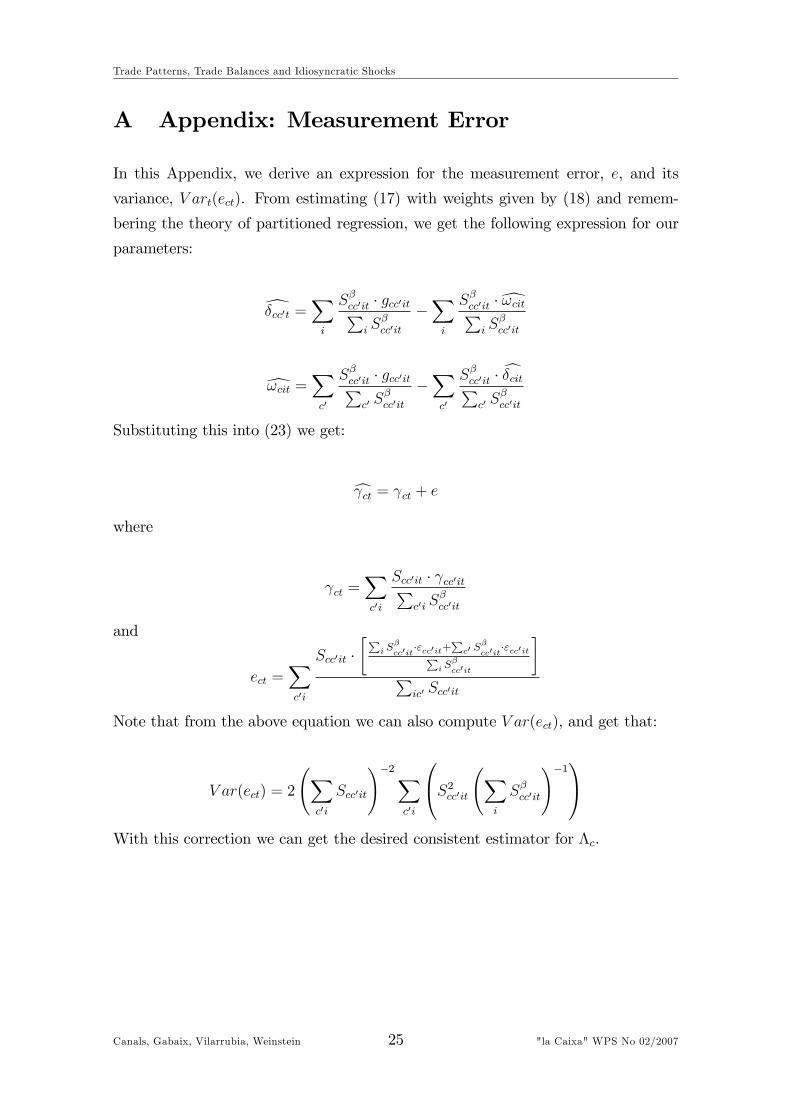
In this Appendix, we derive an expression for the measurement error, e, and its

variance, V art(ect). From estimating (17) with weights given by (18) and remem-

bering the theory of partitioned regression, we get the following expression for our

parameters:

d�cc0t =Xi

S�cc0it � gcc0itPi S

�cc0it

�Xi

S�cc0it �d!citPi S

�cc0it

d!cit =Xc0

S�cc0it � gcc0itPc0 S

�cc0it

�Xc0

S�cc0it � c�citPc0 S

�cc0it

Substituting this into (23) we get:

c ct = ct + ewhere

ct =Xc0i

Scc0it � cc0itPc0i S

�cc0it

and

ect =Xc0i

Scc0it ��P

i S�

cc0it�"cc0it+Pc0 S

�

cc0it�"cc0itPi S

�

cc0it

�P

ic0 Scc0it

Note that from the above equation we can also compute V ar(ect), and get that:

V ar(ect) = 2

Xc0i

Scc0it

!�2Xc0i

0@S2cc0it X

i

S�cc0it

!�11AWith this correction we can get the desired consistent estimator for �c.



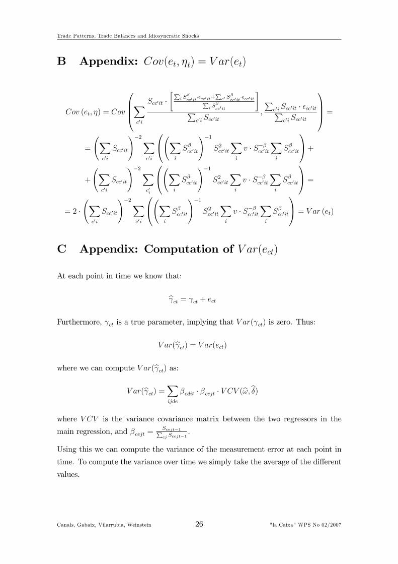
B Appendix: Cov(et; �t) = V ar(et)

Cov (et; �) = Cov

0BB@Xc0i

Scc0it ��P

i S�

cc0it��cc0it+Pc0 S

�

cc0it��cc0itPi S

�

cc0it

�P

c0i Scc0it;

Pc0i Scc0it � �cc0itP

c0i Scc0it

1CCA =

=

Xc0i

Scc0it

!�2Xc0i

0@ Xi

S�cc0it

!�1S2cc0it

Xi

v � S��cc0itXi

S�cc0it

1A++

Xc0i

Scc0it

!�2Xc0i

0@ Xi

S�cc0it

!�1S2cc0it

Xi


S�cc0it

1A =

= 2 � X

c0i

Scc0it

!�2Xc0i

0@ Xi

S�cc0it

!�1S2cc0it

Xi


S�cc0it

1A = V ar (et)

C Appendix: Computation of V ar(ect)

At each point in time we know that:

b ct = ct + ectFurthermore, ct is a true parameter, implying that V ar( ct) is zero. Thus:

V ar(b ct) = V ar(ect)where we can compute V ar(b ct) as:

V ar(b ct) =Xijde

�cdit � �cejt � V CV (b!;b�)where V CV is the variance covariance matrix between the two regressors in the

main regression, and �cejt =Scejt�1Pej Scejt�1

.

Using this we can compute the variance of the measurement error at each point in

time. To compute the variance over time we simply take the average of the di¤erent

values.



Figure1:RatioofTop5IndustriestoTotalTrade.ConcentrationofExportsandImportsbyIndustry.Source:NBER-UCD-

StatisticsCanadaTradeData,1970-1997



Figure2:RatioofTop5TradingPartnerstoTotalTrade.ConcentrationofExportsandImportsbyTradingPartner.Source:

NBER-UCD-StatisticsCanadaTradeData,1970-1997



Figure3:RatioofTop1%

andTop5%

BilateralTradeFlowstoTotalExports.Source:NBER-UCD-StatisticsCanada,Trade

Data1970-1997



Figure4:RatioofTop1%

andTop5%

BilateralTradeFlowstoTotalImports.Source:NBER-UCD-StatisticsCanadaTrade

Data,1970-1997



Table 1: Concentration Ratios for all Bilateral Trade Flows

In % Exports ImportsCountry Top 1% Top 5% Top 10% Top 1% Top 5% Top 10%Canada 95.4 99.6 100.0 94.8 99.8 100.0USA 75.0 96.0 99.3 88.1 99.5 100.0Mexico 94.7 99.8 100.0 91.9 99.8 100.0Japan 86.1 98.6 99.8 89.6 99.7 100.0

South Korea 90.7 99.5 100.0 92.4 99.9 100.0Belgium-Luxembourg 86.2 97.4 99.4 87.7 99.5 100.0

Denmark 79.7 97.8 99.7 79.7 99.1 100.0France 68.3 91.9 97.6 83.6 98.9 99.9Germany 78.5 96.9 99.2 81.1 99.1 100.0Greece 81.9 99.0 100.0 83.8 99.4 100.0Ireland 87.3 99.3 100.0 89.0 99.8 100.0Italy 76.0 96.2 99.2 82.4 99.0 100.0

Netherlands 81.2 96.2 99.0 85.5 99.3 100.0Portugal 84.3 98.9 100.0 86.6 99.7 100.0Spain 76.1 96.4 99.4 86.4 99.5 100.0

United Kingdom 71.1 94.6 98.6 80.2 98.9 100.0Austria 80.8 98.2 99.8 87.1 99.8 100.0Finland 83.9 99.2 100.0 78.4 99.3 100.0Iceland 83.5 99.0 100.0 71.2 98.6 100.0Norway 88.0 99.0 99.9 80.6 99.4 100.0Sweden 81.8 98.5 99.9 81.6 99.4 100.0

Switzerland 77.9 97.5 99.6 87.9 99.6 100.0Australia 86.8 99.4 100.0 86.3 99.5 100.0

New Zealand 85.3 99.5 100.0 84.3 99.2 100.0Mean 82.5 97.8 99.6 85.0 99.4 100.0Median 82.7 98.5 99.8 85.9 99.5 100.0

Each cell contains the 1971-1997 average of the proportion of the top 1%, 5%, and10% of bilateral trade �ows with respect to the total �ows.Source: NBER - UCD - Statistics Canada Trade Data, 1970-1997



Table 2: Concentration Ratios for Top 25 and Top 100 Bilateral Trade Flows

In % Exports ImportsCountry Top 25 Top 100 Top 25 Top 100Canada 89.3 96.2 85.9 96.6USA 52.1 77.0 67.5 90.0Mexico 88.8 97.4 83.8 97.4Japan 67.7 88.3 68.2 92.0

South Korea 75.6 92.9 79.6 96.4Belgium-Luxembourg 66.3 87.4 62.5 90.7

Denmark 52.6 82.2 58.4 89.7France 42.8 70.3 57.5 86.1Germany 52.1 80.1 52.2 84.0Greece 61.6 88.3 66.2 91.1Ireland 70.0 90.6 75.1 94.7Italy 51.4 78.0 59.0 85.8

Netherlands 60.0 82.7 59.6 88.3Portugal 62.9 88.4 66.8 93.4Spain 53.2 78.8 64.1 89.3

United Kingdom 45.0 72.7 52.2 83.7Austria 59.6 85.1 70.5 92.3Finland 64.6 89.4 60.8 91.1Iceland 90.3 99.4 67.6 95.4Norway 74.4 92.4 59.9 92.4Sweden 55.7 84.9 58.0 90.3

Switzerland 55.1 81.7 65.0 91.9Australia 65.3 90.2 68.9 92.6

New Zealand 68.1 92.5 73.2 93.8Mean 63.5 86.1 65.9 91.2Median 62.2 87.8 65.6 91.5

Each cell contains the 1971-1997 average of the proportion for the largest 25 or 100bilateral trade �ows with respect to the total �ows.Source: NBER - UCD - Statistics Canada Trade Data, 1970-1997



Table 3: Her�ndhal Index for Industry Flows

Country Exports ImportsCanada 0.21 0.18USA 0.08 0.15Mexico 0.30 0.11Japan 0.21 0.24

South Korea 0.25 0.17Belgium-Luxembourg 0.08 0.08

Denmark 0.06 0.092France 0.06 0.12Germany 0.09 0.09Greece 0.12 0.13Ireland 0.11 0.10Italy 0.10 0.14

Netherlands 0.07 0.11Portugal 0.16 0.12Spain 0.08 0.18

United Kingdom 0.07 0.08Austria 0.08 0.10Finland 0.09 0.08Iceland 0.57 0.10Norway 0.27 0.08Sweden 0.09 0.10

Switzerland 0.08 0.08Australia 0.09 0.10

New Zealand 0.152 0.11Mean 0.14 0.12Median 0.09 0.10

Each cell contains the 1971-1997 average Her�ndahl Index of �ows aggregated byindustry, computed as:

IHct =Xi

�2cit where �cit =

Pc0 Scc0itPc0i Scc0it

Source: NBER - UCD - Statistics Canada Trade Data, 1970-1997



Table 4: Her�ndhal Index for Country Flows








Each cell contains the 1971-1997 average Her�ndahl Index of �ows aggregated bycountry, computed as:

CHct =Xc0

�2cc0t where �cc0t =

Pi Scc0itPc0i Scc0it




Table 5: Her�ndhal Index for Overall Flows








Each cell contains the 1971-1997 average Her�ndahl of overall, computed as:

OHct =Xc0i

�2cc0it where �cit =Scc0itPc0i Scc0it




Table 6: Median and Weighted Idiosyncratic Shocks to Industry Flows

In % Exports ImportsCountry Weighted Avg. Median Weighted Avg. MedianCanada 10 19 10 72USA 5 16 6 33Mexico 14 17 13 32Japan 5 87 7 114

South Korea 11 37 14 125Belgium-Luxembourg 9 24 9 9

Denmark 8 71 11 71France 5 19 8 54Germany 5 22 9 78Greece 9 33 12 29Ireland 13 23 18 109Italy 5 24 8 22

Netherlands 8 14 8 74Portugal 8 12 16 42Spain 6 19 9 24

United Kingdom 5 12 6 6Austria 8 26 12 62Finland 12 34 11 34Iceland 6 30 15 31Norway 11 39 15 33Sweden 7 47 12 90

Switzerland 7 34 10 4Australia 9 28 14 10

New Zealand 12 78 17 98Mean 8.4 31.9 11.2 52.2Median 8.2 25.0 11.1 37.8

For each industry in each country, we compute the standard deviation of the industry�ows�growth rate (de-meaned of the overall growth rate) as:P

i;t(scit � scit�1)� (sct � sct�1)T � 1

We report the median and a weighted average (with the weights being equal to the squareroot of total �ows in each industry).Source: NBER - UCD - Statistics Canada Trade Data, 1970-1997



Table 7: Median and Weighted Indiosyncratic Shocks to Country Flows

In % Exports ImportsCountry Weighted Avg. Median Weighted Avg. MedianCanada 8 3 8 3USA 6 2 7 3Mexico 10 14 9 26Japan 8 2 10 3

South Korea 13 13 15 9Belgium-Luxembourg 6 2 8 3

Denmark 8 4 8 6France 4 2 7 2Germany 5 2 7 2Greece 12 6 12 4Ireland 13 5 9 3Italy 5 2 8 3

Netherlands 6 2 8 2Portugal 6 7 7 3Spain 8 3 10 3

United Kingdom 5 1 7 2Austria 10 2 9 3Finland 12 11 11 7Iceland 9 27 9 11Norway 10 8 8 4Sweden 8 5 9 10

Switzerland 8 2 10 9Australia 7 26 7 37

New Zealand 15 5 10 4Mean 8.4 6.5 8.8 6.8Median 7.8 3.1 8.7 3.3

For each country�s trading partner, we compute the standard deviation of the tradingpartner�s �ows�growth rate (de-meaned of the overall growth rate) as:P

c0;t(scc0t � scc0t�1)� (sct � sct�1)T � 1

We report the median and a weighted average (with the weights being equal to the squareroot of total �ows in each industry).Source: NBER - UCD - Statistics Canada Trade Data, 1970-1997



Table 8: Lambda Ratio using Industry and Country Dummies

In % Exports ImportsCountry b�c 95% Conf. Int. �c 95% Conf. Int.Canada 66 [33,100] 51 [26,100]USA 13 [6,100] 32 [16,100]Mexico 44 [22,100] 32 [16,100]Japan 18 [9,100] 40 [20,100]

South Korea 30 [15,100] 76 [39,100]Belgium-Luxembourg 27 [14,100] 27 [14,100]

Denmark 21 [11,100] 38 [19,100]France 6.4 [3,100] 15 [7.8,100]Germany 8.2 [4,100] 10 [4.8,100]Greece 48 [24,100] 30 [15,100]Ireland 127 [64,100] 45 [23,100]Italy 14 [7,100] 39 [20,100]

Netherlands 16 [8,100] 23 [11,100]Portugal 21 [11,100] 29 [15,100]Spain 26 [13,100] 35 [18,100]

United Kingdom 13 [7,100] 15 [7.4,100]Austria 17 [9,100] 33 [17,100]Finland 32 [16,100] 17 [8.7,100]Iceland 54 [27,100] 47 [24,100]Norway 60 [30,100] 23 [11,100]Sweden 21 [10,100] 25 [13,100]

Switzerland 10 [5,100] 19 [9.4,100]Australia 62 [31,100] 21 [11,100]

New Zealand 60 [30,100] 46 [23,100]Median 24 31

b�c measures the fraction of the variance of exports/imports growth attributable toidiosyncratic shocks, formally:

b�c = V art (c�ct) + V art (ect)V art (c�ct) + V art (c ct)



Table 9: Lambda Ratio using Mid-Point Growth Rates

In % Exports Imports TradeCountry 95% Conf 95% Conf 95% Confb�c Int. b�c Int. b�c Int.Canada 48 [24,100] 37 [19,100] 57 [29,100]USA 13 [6,100] 27 [14,100] 48 [24,100]Mexico 33 [17,100] 18 [9,100] 42 [21,100]Japan 24 [12,100] 40 [20,100] 60 [30,100]

South Korea 37 [18,100] 67 [34,100] 46 [23,100]Belgium-Luxembourg 20 [10,100] 20 [10,100] 71 [36,100]

Denmark 17 [8,100] 31 [16,100] 60 [30,100]France 6 [3,100] 15 [8,100] 63 [32,100]Germany 7 [3,100] 8 [4,100] 57 [29,100]Greece 52 [26,100] 35 [18,100] 67 [34,100]Ireland 71 [36,100] 52 [26,100] 52 [26,100]Italy 11 [5,100] 34 [17,100] 64 [32,100]

Netherlands 14 [7,100] 15 [8,100] 55 [28,100]Portugal 22 [11,100] 24 [12,100] 56 [28,100]Spain 20 [10,100] 33 [16,100] 61 [31,100]

United Kingdom 11 [6,100] 17 [9,100] 53 [27,100]Austria 11 [6,100] 26 [13,100] 60 [30,100]Finland 30 [15,100] 15 [7,100] 45 [23,100]Iceland 156 [79,100] 80 [40,100] 50 [25,100]Norway 48 [24,100] 20 [10,100] 51 [26,100]Sweden 16 [8,100] 25 [13,100] 54 [27,100]

Switzerland 7 [4,100] 14 [7,100] 63 [32,100]Australia 56 [28,100] 14 [7,100] 38 [19,100]

New Zealand 52 [26,100] 102 [52,100] 40 [20,100]Median 21 26 55

b�c measures the fraction of the variance of exports/imports growth attributable toidiosyncratic shocks, formally:

b�c = V art (c�ct) + V art (ect)V art (c�ct) + V art (c ct)



Table 10: Cumulative Export Share by Top Firms

In % In Sample Total ExportsTop 1983 1999 1983 19991 9.5 10.6 6.7 8.72 16.8 15.3 11.8 12.63 20.7 19.5 14.6 16.14 24.5 23.6 17.2 19.55 28.2 27.7 19.8 22.910 40.7 40.6 28.6 33.515 49.5 49.0 34.8 40.420 56.5 55.0 39.8 45.425 62.2 59.5 43.8 49.150 75.7 72.5 53.3 59.8

The number in cell each represents the percentage of exports by top �rms withrespect to total exports. In the �rst two columns the percentage is with respectto total exports within our sample while in the third and fourth columns it is withrespect to total exports as reported by OECD.Source: DBJ, OECD.



Table 11: Average Growth Rate and Volatility for the Largest Japanese ExportingFirms

In %Company Av. Idiosyncratic Std. Dev of

Growth Rate Idiosyncratic Growth RatesToyota Motor Corp. 3.10 6.80Nissan Motor Co., Ltd. -2.98 4.96Honda Motor Co., Ltd. 0.63 6.04Matsushita Electric Industrial Co.,Ltd. 0.32 11.94Mazda Motor Corp. -1.47 7.75Sony Corp. 2.09 9.09Hitachi,Ltd. -2.22 7.36Toshiba Corp. 1.33 11.62Canon Inc. 4.40 8.18Nippon Steet Corp. -0.06 6.11Nec Corp. 0.43 9.57Mitsubishi Motors Corp. 0.29 5.17Mitsuboshi Heavy Industries, Ltd. 1.43 10.00Isuzu Motors Ltd. 2.29 15.96Sharp Corp. -0.80 7.17Mitsubishi Electric Corp. 0.75 7.51Suzuki Motor Corp. 2.91 13.01Fujitsu Ltd. 7.94 20.24NKK Corp. 0.59 12.84Victor Co. of Japan, Ltd. -4.37 9.11Sumitomo Metal Industries, Ltd. -0.61 6.91Sanyo Electric Co., Ltd. -6.28 7.65Kawasaki Steel Corp. 0.36 5.98Fuji Heavy Industries, Ltd. 2.72 17.79Kawasaki Heavy Industries, Ltd. -0.05 14.22

Median (25) 8.18W. Avg (25) 8.91Median (All) 21.47W. Avg. (All) 37.91

For each �rm, the idiosyncratic growth rate is de�ned as (sfit � sit), its average as1T

Pt(sfit � sit), and its standard deviation as 1

T�1P

t(sfit � sit)


trade patterns, trade balances and idiosyncratic shocks - caixabank research · 2019-03-05 ·...

Documents