Trade Policy-Making in a Model of LegislativeBargaining∗

Levent Celik† Bilgehan Karabay‡ John McLaren§

December 10, 2011

Abstract

In democracies, trade policy is the result of interactions among many agents withdifferent agendas. In accordance with this observation, we construct a dynamic modelof legislative trade policy-making in the realm of distributive politics. An economyconsists of different sectors, each of which is concentrated in one or more electoraldistricts. Each district is represented by a legislator in the Congress. Legislative pro-cess is modeled as a multilateral sequential bargaining game a la Baron and Ferejohn(1989). Some surprising results emerge: bargaining can be welfare-worsening for allparticipants; legislators may vote for bills that make their constituents worse off; iden-tical industries will receive very different levels of tariff. The results pose a challengeto empirical work, since equilibrium trade policy is a function not only of economicfundamentals but also of political variables at the time of congressional negotiations –some of them random realizations of mixed bargaining strategies.

Keywords: Trade Policy; Multilateral Legislative Bargaining; Political Economy; Dis-tributive Politics.JEL classification: C72, C78, D72, F13.

∗We would like to thank to Gerald Willmann, Kresimir Zigic and the participants at the 6th AustralianTrade Workshop, the 7th Asia Pacific Trade Seminars, the University of Auckland Research Workshop andCERGE-EI research seminar for helpful comments. We are also grateful to CERGE-EI, the University ofVirginia and the University of Auckland for their hospitality during the authors’ visits. This research wassupported by a grant (project reference number 3625352/9554) from the University of Auckland FacultyResearch Development Fund. All opinions expressed are those of the authors and have not been endorsedby the University of Auckland. All errors are our own.†CERGE-EI (a joint workplace of the Center for Economic Research and Graduate Education, Charles

University, and the Economics Institute of the Academy of Sciences of the Czech Republic), Politickychveznu 7, 111 21, Prague 1, Czech Republic. E-mail: celik@cerge-ei.cz. URL: http://home.cerge-ei.cz/celik.‡Department of Economics, University of Auckland, Owen G. Glenn Building, 12 Grafton Road, Auckland

1010, New Zealand. E-mail: b.karabay@auckland.ac.nz. URL: http://bilgehan.karabay.googlepages.com.§Department of Economics, University of Virginia, P.O. Box 400182, Charlottesville, VA 22904-4182.

E-mail: jmclaren@virginia.edu. URL: http://people.virginia.edu/˜jem6x.

1 Introduction

“But to introduce a tariff bill into a congress or parliament is like throwing a

banana into a cage of monkeys. No sooner is it proposed to protect one industry

than all the industries that are capable of protection begin to screech and scramble

for it. They are, in fact, forced to do so, for to be left out of the encouraged ring

is necessarily to be discouraged.” – Henry George (1886).

Attempts by economists to understand the process of trade policy formation1 have evolved

from approaches based on electoral competition (Mayer, 1984), through lobbying (Findlay

and Wellisz, 1982) and influence-peddling (Grossman and Helpman, 1994), to more recent

work focussed on the workings of legislative assemblies (such as Grossman and Helpman,

2005 and Willmann, 2004).

In this paper, we add an important element to the analysis: dynamic, non-cooperative

congressional bargaining. Models that focus on congressional decision making assume a

unified majority party writes and passes a bill, such as Grossman and Helpman (2005), or

that implicit cooperative congressional bargaining maximizes joint utility of representatives,

as in Willmann (2004). These approaches provide simplicity by clearing away by assumption

many of the features that make trade policy complicated in practice. By contrast, in the

model we propose here, in order to move tariffs from the status quo, the member of the

Congress who can set the agenda must propose a trade bill and find a majority coalition

willing to support it. In choosing how to vote, each member considers the uncertainty over

who will have agenda-setting power next, and thus over what tariff bill will emerge down

the road if the current bill fails. In this setting, a number of features emerge that are quite

different from what other models offer:

(i) The trade policy that emerges will depend on which member of the Congress has

agenda-setting power, apart from the fundamentals generally accounted for in empirical

1There is an extensive literature on trade policy formation; see Rodrik (1995) and Nelson (1999) for areview.

1

work – both economic fundamentals (industry size, elasticities of demand, and so on) and

institutional fundamentals (political organization of the industry). Indeed, since omnibus

trade bills are passed infrequently, this implies that, at any given date, the structure of tariffs

across industries can be largely the result of who chaired what committee, for no matter how

brief a period, many years ago.

(ii) The equilibrium of the bargaining game is typically in mixed strategies. Conditional

on fundamentals and the identity of the agenda-setter, the outcome is random because the

agenda setter chooses randomly between industries to attract to the winning coalition. The

randomness of this choice is a deep feature of the model that results from the dynamic nature

of the game – specifically, the possibility of multiple rounds of bargaining after the current

round if no bill passes; a static game would have no reason for randomness. As a result,

even conditional on fundamentals and also on the identity of congressional leadership at the

time of the bill’s passage, empirical work explaining the determinants of tariffs might need

to control for the identity of the winning coalition, perhaps proxied by the members who

voted in favor.

(iii) Because of the uncertainty about the future agenda setter and future proposals that

will come to the table, in many cases a member of the Congress will vote for a bill that is

worse for her constituents than the status quo. Again, this is a feature of the dynamic nature

of the model and would disappear in a static version.

[+++]One can think of this as a model of congressional trade-policy making in the days

before Congress routinely delegated trade authority to the executive branch through the

Reciprocal Trade Agreements Act of 1934 or the later Fast Track Authority. Indeed, one

can think of our model as examining exactly the sort of problems that led Congress to begin

delegating trade-policy authority. This interpretation is explored in depth in Celik, Karabay

and McLaren (2011). Given this interpretation, the key elements of the model can be seen

in the rough and tumble of trade-bill formation in historical practice. Consider the 1880’s

in the United States, a period in which trade policy was perhaps the most contentious and

vigorously debated issue of the day and the issue on which at least one national election

2

was decided. Consider three central elements to our story, each of which requires a dynamic

model. (i) Uncertainty about the agenda setter. The main agenda setter in the US House

of Representatives for trade bills is the chair of the Ways and Means Committee, appointed

by the Speaker of the House. In 1883, the Speaker was Samuel Randall, a Democrat from

Pennsylvania, an ardent protectionist allied with iron and other industries of his home state.

He was challenged in that year for the position of Speaker by John Carlisle of Kentucky, a

Democrat from a rural area committed to much lower tariffs all around. The battle for the

chairmanship was intense, and Carlisle surprised everyone by pulling an upset victory (Tar-

bell, 1911, p. 137)). Carlisle appointed a moderate free-trader, William Morrison of Illinois,

to the Chairmanship of Ways and Means. Later, the agenda-setter changed unpredictably

once again, when Morrison in 1886 lost his re-election campaign and was replaced at Ways

and Means by a stauncher free trader, Roger Mills of Texas (Tarbell, 1911, p. 155). The

agenda-setter changed more dramatically in 1888, when Republicans won a majority in the

House, and staunch protectionists seized control from the ardent free traders. Thus, in just

a few years, the agenda-setting power changed hands several times, among politicians with

very different policy preferences. (ii) The proposed trade bill changes dramatically with the

identity of the agenda setter. Several different trade bills were proposed during this period,

and the proposed bills changed character rapidly with changes in the agenda setter. For

example, the Mills bill of 1888 lowered tariffs across the board, while the McKinley tariff bill

passed by the new Republican house in 1890 raised tariffs sharply for almost every industry

(Tarbell, 1911, pp. 188-206). (iii) The coalition supporting a proposed bill does not depend

merely on party, but on the contents of the bill. Randall, for example, had built a coalition

of supporters for his protectionist agenda that included a wide range of Republicans and a

number of Democrats willing to buck their party’s dominant free-trade ideology (Tarbell,

1911, p. 137). (iv) Members of the Congress vote strategically, sometimes voting for a pro-

posal that will make things worse for their constituents, because they are concerned that the

next proposal might be even worse. This can be seen in the decision by Randall’s supporters

in the House to support the Mills tariff reduction bill ‘with heavy hearts’ as likely the best

3

they could obtain, although it reduced tariffs rather than raised them as their constituents

desired (Tarbell, 1911, pp. 164-165).

Thus, the main elements of our model are very much in play in the real world of con-

gressional tariff-setting. Now, to sketch our model in more detail. We consider a small

open economy that accommodates four industries, one that produces numeraire homoge-

neous good using labor alone and three manufacturing industries that employ sector-specific

capital alone. There are N electoral districts (constituencies),2 each of which hosts one man-

ufacturing industry along with the numeraire good industry. Individuals who reside in the

same district are identical and each one is endowed with one unit of labor and one unit of

capital to be used in the manufacturing industry located in that district. As a result, there

is a potential conflict among districts based on (manufacturing) industry attachment.3

Each district is represented by a legislator in the legislature (Congress).4 Each legislator

cares only about the welfare of her own district,5 and the welfare of a district is closely

related to the industry located in it. In our model, trade policy implies any tariff or subsidy

levied on any sector’s output.6 This setup is consistent with distributive politics since an

increase in the price of a particular good (say, due to protection) will be beneficial only to

those districts that produce it, but will be costly to the whole economy due to its negative

effect on consumption.

We analyze the legislative game as a sequential model of multilateral bargaining with

a simple majority rule a la Baron and Ferejohn (1989). This approach to congressional

2Constituencies are usually described in geographic terms in studies of the Congress; see Anderson andBaldwin (1987), Irwin and Kroszner (1999) and Lindsay (1990). This is intuitive since the electorate formembers of Congress is defined geographically.

3Magee (1978), in his study of testimony on trade legislation, finds strong evidence for sector-basedpolitical activity. Moreover, in other studies, capital and labor are found to be relatively immobile overpolitically plausible time horizons; see Nelson (2007), footnote 4.

4We do not model the election of legislators in this paper. However, the results would not change as longas there is no commitment to party loyalty.

5This is in line with the empirical literature; see, among others, Baldwin (1976; 1985), Hiscox (2002),Fordam and McKeown (2003) and Ladewig (2006). The underlying assumption is that each legislator mustcalculate how voters in her district will respond to a particular trade policy in order to maximize herprobability of re-election.

6Here, we use tariffs as a measure of protection. In reality, non-tariff barriers (NTBs) are also used andvery closely related to tariffs as documented by Ray (1981) and Marvel and Ray (1983).

4

bargaining has borne much fruit in the political economy of public finance (see, among

others, Baron, 1993; Primo, 2006 and Battaglini and Coate, 2007), but to our knowledge it

has not yet been used to analyze trade policy. Each period, a legislator is selected randomly

to propose a tariff bill.7 To pass a bill, the proposer must create a coalition of supporting

legislators large enough to form a majority, in which case the bill goes into effect and the

legislature adjourns. Otherwise, the status quo trade policy prevails and the process is

repeated with a new legislator (possibly the same as in the previous period). In her voting,

a legislator compares the benefits accruing to her district from the current proposal to the

value of continuing to the next stage.

A new trade policy affects individuals’ welfare through three distinct channels. First, all

individuals earn capital rent through the sector-specific capital they own. A higher tariff for

a particular good, therefore, benefits those individuals who have a stake in that industry.

Second, individuals derive utility from consumption. Thus, a higher tariff on any good lowers

their consumer surplus. Finally, individuals share the revenue (positive or negative) from all

taxes and subsidies imposed through trade policy. Keeping these three effects in mind will

be helpful in interpreting the results.

A closer look at our findings yields the following observations. First, the ex ante expected

benefit an industry receives from congressional bargaining is affected by the industry’s dis-

persion (i.e., the number of electoral districts an industry operates in).8 To focus on the

pure dispersion effect, consider the thought experiment in which each industry produces the

same output, but they differ in the number of districts in which they operate. We show first

that, independent of other factors, trade protection is higher for industry i than industry j

if industry i representatives constitute a majority in the Congress. This makes sense; if an

7Random recognition is a convenient way to model the uncertainty that legislators face, i.e., they do notknow exactly which coalitions will form in the future if the current coalition fails to enact the legislation.Although the purely random selection is of course an abstraction, the uncertainty regarding the agendasetter is important in practice, as illustrated by the historical example discussed above, and this convenientabstraction is used in an enormous literature following Baron and Ferejohn (1989).

8Busch and Reinhardt (1999) argue that geographical concentration is different from political concen-tration. Our focus is on industry spread across political districts, hence more in line with the definition ofpolitical concentration. However, for simplicity, we do not distinguish between these two terms.

5

industry is dispersed enough to have a majority representation in the Congress, then it will

receive more protection due to its agenda-setting power.9

However, we show that if no industry has a majority in the Congress, more disperse

industries have no advantage ex ante over less disperse industries. The reason is that a more

disperse industry has a better chance of holding agenda-setting power (since it controls more

seats), and so it can drive a harder bargain when it is in a coalition. Consequently, when

it is not the agenda setter, it has a much lower probability of being included in a coalition.

This is a subtlety that as far as we know has not been investigated in empirical work.

Second, in case no industry has majority representation in the Congress, the ex ante

expected benefit an industry receives from Congressional bargaining is determined by that

industry’s total output. In particular, larger industries that produce more output tend to

benefit less from congressional negotiations over tariffs than smaller industries. The reason

is that such an industry will generate fewer imports (since it will satisfy more of domestic

demand from domestic production), and so the tariff revenue produced by a given tariff will

be small; but this means that if a large industry is a member of the coalition that forms the

tariff bill, the coalition partner will receive little benefit from a tariff on the large industry,

and so will be unwilling to agree to a high tariff.

Third, in addition to these factors, the status quo tariffs also matter.10 In particular, if

the initial protection for an industry is already high compared to other industries, then there

is less room for that industry to improve over its status quo welfare since it is closer to its

ideal protection level than others.

[+++]This paper draws on a number of related contributions. Obviously, we have de-

9We do not have political parties in our model, so the only way an industry can hold sway over a majorityof districts is to have voters with an economic stake in that industry residing in a majority of districts. If wehad parties in the model, it could also be possible for an industry to gain influence by being concentrated indistricts held by the majority party, even if the industry is geographically concentrated. Evidence for this isprovided by Fredriksson, Matschke and Minier (2011), who show, using U.S. tariff data from 1993, that anindustry receives positive protection if it is relatively concentrated in districts held by the majority party.An extension to allowing for parties could be of interest, but is beyond the scope of the present paper.

10The status quo tariffs matter for welfare effects even though in the limiting case where the members ofCongress are very patient, they do not matter for the final level of tariffs. The effect of historical patternsof protection on current protection is documented by Lavergne (1983) and Ray and Marvel (1984).

6

rived the overall bargaining structure from Baron and Ferejohn (1989), which appears not

to have been used in international economics previously. It should be emphasized, however,

that extending their model of pure distribution to trade policy is not straightforward. Dis-

tortionary trade policy affects not only the division of the pie, but the size of the pie, and

indeed we will see that payoffs are concave in the tariffs, so the randomization created by

congressional bargaining tends to lower welfare for all. In addition, considerable complexity

is created by the presence of a non-trivial status quo (given by trade with initial tariffs,

which may differ across industries), unlike in the original models. We are able to show that

in the limit with very patient players (but only in the limit) these status quo tariffs do not

matter for the outcome.[+++]

Our model is also closely related to Willmann (2004), McLaren and Karabay (2004) and

Grossman and Helpman (2005). In Willmann’s (2004) citizen-candidate model, heteroge-

neous districts behave strategically such that they have a tendency to choose candidates

that are more protectionist than the district median. From a regional perspective, voters

prefer a positive tariff, ignoring the tariff costs imposed on other districts. In contrast, from

a national perspective, these tariff costs are internalized and, therefore, each district’s rep-

resentative has to make a compromise. Knowing this compromise, in each district, voters

in the first stage (namely, regional election stage) choose someone who is more protectionist

than the median voter of that district.

McLaren and Karabay (2004) extend the standard median-voter framework to a rudimen-

tary model of a government by assembly where parties compete by making binding election

promises. In their model, the equilibrium tariff turns out to be the optimal tariff of the

median voter in the median congressional district. They show that import-competing inter-

ests are more likely to receive protection if they are moderately geographically concentrated

(neither too concentrated nor too dispersed). They also conclude that majoritarian systems

tend to be more protectionist than presidential systems.

Grossman and Helpman (2005) consider a three-stage game. First, parties announce their

policy platforms, then elections take place, and in the final stage, a particular trade policy

7

is adopted. In this model, the lack of full commitment to announced party policies creates

protectionist bias as long as districts differ in their capital endowments.

Willmann (2004) models the trade policy determination as a joint welfare maximization

of all legislators whereas Grossman and Helpman (2005) model it as a joint welfare max-

imization of majority party legislators. On the other hand, McLaren and Karabay (2004)

employ an election framework in which trade policy is predetermined. The common property

of all of these papers is that there is not much scope for legislative procedures. In contrast,

non-cooperative legislative bargaining is the core force behind trade policy formation in our

model.

The rest of the paper is organized as follows. In the next section, we describe the basic

model. In section 3, equilibrium is characterized. We discuss possible extensions in section

4. Section 5 concludes the analysis.

2 Model

Consider a small open economy populated with a unit measure of individuals living in N

districts (where N > 3 and divisible by 3). There are M = 4 industries: one that supplies

a homogeneous numeraire good (good 0) produced with labor alone, and three others, each

of which supplies a homogenous manufacturing good (goods 1 through 3) produced with

sector-specific capital alone.11 In particular, we assume that the production technology

for good 0 yields 1 unit of output per unit of labor input, and the technology for each

manufacturing good takes the following form: fi(Ki) = θKi, where Ki and θ denote the

amount of the sector-specific capital used in sector i and the economy-wide productivity

parameter, respectively. (Unless specified otherwise, we use index letters (i, j, k) only for

the manufacturing goods.)

Each district is composed of a homogeneous population; each individual residing in a

given district is endowed with one unit of labor and also one unit of the same type of sector-

11We limit the number of manufacturing industries to three for simplicity, as in Grossman and Helpman(2005). Results remain qualitatively similar for more than three manufacturing industries. There are,however, many more possibilities (of coalition formation) to consider. See section 4 for further remarks.

8

specific capital.12, 13 Let the number of districts producing good i be denoted by ni such that

n1 + n2 + n3 = N . Without loss of generality, we assume that n1 ≥ n2 ≥ n3. Districts that

produce the same manufacturing good are populated by the same number of individuals. To

save on notation, we let Ki denote both the total amount of type-i capital in a type-i district

and the total number of individuals residing in a type-i district. Given that the population

is of unit mass,3∑i=1

niKi = 1.14 Let qi denote the amount of good i produced in a district

that hosts industry i, and Qi denote the total amount of good i produced in the economy.

Therefore, we have qi = θKi and Qi = niqi.15 This implies that

3∑i=1

Qi = θ3∑i=1

niKi = θ. In

addition, let p∗i and pi represent, respectively, the exogenous world price of good i and its

domestic price. On the other hand, the numeraire good, good 0, has a world and domestic

price equal to 1 (see footnote 19). Thus, the total rent that accrues to capital in district i is

piqi = θpiKi, and the total labor income earned in district i is Ki.

Each individual has an identical, additively separable quasi-linear utility function given

by

u = c0 +3∑i=1

ui (ci) ,

where c0 is the consumption of good 0 and ci represents the consumption of good i = 1, 2, 3.

We assume that ui (ci) = Rici− (c2i /2), where Ri > 0 and assumed to be sufficiently large.16

With these preferences, the domestic demand for good i, implicitly defined by u′i (d(pi)) = pi,

is given by d(pi) = Ri− pi. The linearity of demand is not crucial for the main results of our

12Our results carry over even if more than one industry is allowed in each district as long as each residentstill holds only one sector-specific capital and in every district there is one industry with majority repre-sentation. This is true since each legislator will follow the interests of the median voter, who belongs to aparticular industry under the conditions assumed here.

13We do not model the location choice of a particular industry, rather we take it as given. However, weacknowledge that this choice may depend on the political influence an industry can exert in each location.

14We allow only those districts that produce different goods to differ in the number of citizens residing.This is done to simplify the notation. Alternatively, it is possible to allow each district (even the onesproducing the same good) to be populated by different number of individuals. All of our results continue tohold.

15To make things simple and analytically tractable, aggregate output of each industry is perfectly inelasticin our setup. This is merely to eliminate some complexity, but there is some evidence that supply elasticitiestend to be quite low in practice; see Marquez (1990) and Gagnon (2003).

16To be more precise, we require Ri > p∗i + θ −Qi. This ensures that demand for good i is positive at allprices that may occur in legislative bargaining. We also require p∗i > Qi for each price to be positive. Seesection 3 for the determination of optimal tariffs (hence optimal prices).

9

paper, but it simplifies the analysis and permits a closed-form solution. The indirect utility

of an individual with income y is y + s (p), where p = (p1, p2, p3) is the vector of domestic

prices,17 and s (p) =∑3

i=1 [ui (d(pi))− pid(pi)] is the resulting consumer surplus.

Each district is represented by a single legislator who is concerned only with the welfare

of her own district. A district’s welfare is the aggregate utility of all individuals in that

district, which is equal to the total income plus the district’s share in total consumer surplus

and total tariff revenue (or subsidy cost) for each good. Hence, a district that produces good

i has a total welfare (for i 6= j 6= k)

Wi(p) = Ki + piθKi +Ki

∑l=i,j,k

(Rl − pl)2

2+Ki

∑l=i,j,k

[(pl − p∗l ) (Rl − pl −Ql)] , (1)

where the first term is the district’s labor income (equal to one unit of good 0 output per

person), the second term is the capital rent, the third term is the consumer surplus captured

by that district (recall that Ki also represents the population share of a district that produces

good i), and the last term is its share of tariff revenue (or subsidy cost).18 In addition, we

denote wi(p) as the welfare of an individual with a stake in industry i, hence

wi(p) = 1 + piθ +∑l=i,j,k

(Rl − pl)2

2+∑l=i,j,k

[(pl − p∗l ) (Rl − pl −Ql)] . (2)

We consider an infinite-horizon model. Every period, there is a set of prices at which in-

dividuals make their production and consumption decisions, and enjoy the resulting welfare.

The legislature can change the prevailing status quo, ps = (ps1, ps2, p

s3), by changing the do-

mestic price of any good via legislative bargaining. We restrict the set of policy instruments

available to the legislature and allow only for trade taxes and subsidies. A domestic price in

excess of the world price implies an import tariff for an import good and an export subsidy

for an export good. Domestic prices below world prices correspond to import subsidies and

export taxes.19

17We restrict each domestic price to satisfy: 0 ≤ pi < pi, where pi = p∗i +(Ri−p∗i )

2+(θ−Qi)2

2(θ−Qi). These limits

ensure that we get an interior solution in prices.18We assume that tariff revenue (or subsidy cost) is distributed equally as a lump-sum transfer to each

individual.19Without loss of generality, we assume that the tariff/subsidy on good 0 is equal to 0. Any tariff vector τ ′

10

The timing of the trade-policy formation game in our model is based on the Baron-

Ferejohn bargaining framework. This is a game of complete information. At the start of each

period (before any production or consumption takes place),20 a legislator is selected randomly

(with equal probability for each legislator) to propose a tariff vector.21 If the proposal receives

a simple majority, it is immediately implemented and the legislature adjourns. Each district’s

welfare thereafter is evaluated at the new prices.22 If the proposal does not receive a majority,

the process is repeated with another legislator (possibly the same as in the previous period)

to propose a new tariff bill. Bargaining continues until a bill is implemented.23 Districts

continue to receive their status quo welfare in every period until an agreement is reached.

There are a couple of things to note. First, it is straightforward to show that the aggregate

welfare, W (p) =∑3

i=1 niWi(p), is maximized at the free trade prices of the three goods.

Hence, if the prices were set by a central authority (such as a President), free trade would

prevail forever. In the current paper, however, we are interested in policy-making by a

legislature. This naturally introduces a conflict of interest among legislators since each

legislator is selfishly interested in maximizing her own district’s welfare. Put another way,

when proposing a trade bill, each legislator weighs the marginal benefits and costs for her

own district but ignores the negative externality imposed on others. Therefore, the resulting

trade policy is inefficient for the economy as a whole.

Second, from equation (1), a manufacturing good affects (through its price) a district’s

yielding domestic prices p′ = p∗+τ ′ with τ ′0 6= 0 can be replaced by τ ′′ ≡ 1p′0

[τ ′−τ ′0p∗] yielding p′′ = p∗+τ ′′

without changing relative prices or any real values. Given that good 0 is the numeraire, this implies thatp′′0 = p∗0 = 1.

20To simplify, we assume that a period in the legislative game coincides with a production/consumptionperiod.

21Therefore, the probability that the proposer represents industry i is equal to ni

N .22Note that once a proposal is accepted, the game ends so that there will be no future proposals. The

underlying assumption is that the legislative bargaining process is too costly to be repeated. Indeed, it ispossible to show that if a new proposal is allowed in every period even after an agreement is reached, thenthe expected welfare of each industry is lower. See section 4 for more on this issue.

23We model the legislative process as an infinite horizon game. According to Osborne and Rubinstein(1994), “a model with an infinite horizon is appropriate if after each period players believe that the gamewill continue for an additional period, while a model with a finite horizon is appropriate if the playersclearly perceive a well-defined final period.” In our setup, there is uncertainty about the exact time whenthe legislative period will end. Therefore, there is no well-defined final period in our game.

11

welfare via three channels. The first one, the rent that accrues to the specific factor, is

present if that good is produced in that district. The second one is the consumer surplus

attained from the consumption of that good. The last one is the tariff revenue (or subsidy

cost) due to trade. The effect of price through the first channel is always positive whereas

it is always negative through the second channel. Its effect through the third channel, on

the other hand, can be positive or negative (in fact the third channel is concave in all three

prices). This is true since good i’s price has two distinct effects on tariff revenue/subsidy

cost: (1) the direct effect (changing price while keeping imports/exports constant), and (2)

the indirect effect through demand. These two effects work in opposite directions. To see

this, assume that good i is an imported good. First, start from a price just above the world

price. As we increase the price, the direct effect leads to an increase in the tariff revenue

whereas the indirect effect leads to a decrease (since import demand goes down). Initially,

the direct effect dominates, and therefore, raising the price raises tariff revenue. When the

price reaches a certain value, the indirect effect starts dominating and the tariff revenue

decreases if we further increase the price.

3 Characterization of equilibrium

In this section, we investigate the properties of the bargaining outcome. As common in

multi-person bargaining problems, there may be many subgame perfect equilibria (SPE)

in this game.24 We focus on stationary subgame perfect equilibrium (SSPE) whereby the

continuation payoffs for each structurally equivalent subgame are the same.25 In a stationary

equilibrium, a legislator who is recognized to make a proposal in any two different sessions

behaves the same way in both sessions (in the case of a mixed-strategy equilibrium, this

means choosing the same probability distribution over offers). Hence, stationary equilibria

24Baron and Ferejohn (1989) show that any outcome (in their game that means any division of the dollar)can be supported as an SPE using infinitely nested punishment strategies as long as there are at least fiveplayers and the discount factor is sufficiently high. Li (2009) shows that even with three players, there is avast multiplicity of SPE.

25Baron and Kalai (1993) argue that stationarity is an attractive restriction since it is the “simplest”equilibrium such that it requires the fewest computations by agents.

12

are history-independent. To make our results as clear as possible, we focus on the case in

which the discount factor (denoted by δ) approaches 1 in the limit.26

For the remainder of the analysis, we let τ = (τ1, τ2, τ3), where τi = pi − p∗i . Therefore,

we can rewrite equation (2) as

wi(τ) = 1 + (p∗i + τi)θ +∑l=i,j,k

(Rl − p∗l − τl)2

2+∑l=i,j,k

τl (Rl − p∗l − τl −Ql) . (3)

Let the per-period equilibrium welfare of a district producing good i, evaluated at the

beginning of a period, before the proposer has been selected, be denoted as Vi. This is also

the per-period equilibrium welfare a district expects in the following period in the event that

the period ends without a bill passed, and so we will also call it the ‘continuation payoff.’

(Recall that we are focussed on the limiting case as δ → 1.) Since a random proposer is

selected every period, the outcome of legislative bargaining depends on the identity of the

proposer. In this sense, the outcome is ex ante uncertain. Hence, we use the ex ante expected

per-person welfare change due to bargaining as the basis for comparison among individuals

with stakes in different sectors. To this purpose, let vi denote the continuation payoff of an

individual with a stake in industry i, thus vi = ViKi

.

When a legislator is recognized to make a proposal, she has an incentive to propose a

tariff bill that will be accepted, since if rejected, she faces the risk that her district might be

worse off with a bill adopted in the future. In equilibrium, in accordance with the “Riker’s

(1962) size principle,” any proposal will be accepted with the minimal number of industries

that constitute a quorum of districts. In other words, the proposer forms a ‘minimum

winning coalition’ by choosing at most one ‘coalition partner.’ This is true since increasing

the number of industries in the winning coalition would increase the costs without increasing

the benefits.

We assume that a legislator votes yes to a proposal if and only if the benefits accruing

to her district from the current proposal is at least as high as the expected payoff it obtains

26This may be interpreted such that the time length between any two offers (sessions) is infinitesimallyshort. See section 4 for the implications of relaxing this assumption.

13

in case the proposal does not pass.27 Suppose a legislator who represents a district that

produces good i is recognized to make a proposal and she proposes a tariff vector τ i. Also,

let τ s = (τ s1 , τs2 , τ

s3 ) describe the vector of status quo trade taxes (or subsidies). Then,

legislators who represent districts that produce good j 6= i would say yes if and only if28

wj(τi)

1− δ≥ wj(τ

s) +δvj

1− δ.

The left-hand side of the above inequality indicates the per-capita discounted total welfare a

district that produces good j obtains at the proposed prices, whereas the right-hand side is

the expected per-capita discounted payoff if bargaining is carried over to the following period

(the status quo welfare for the current period and the continuation welfare thereafter).

The values of vj, ∀j are endogenous, as they are determined by the equilibrium tariff bill

and the equilibrium probability of being in a winning coalition. However, any recognized

legislator will take them as given when designing the tariff bill. Moreover, the recognized

legislator will choose τ such that the constraint is satisfied with equality, which means that

wj(τ) = (1 − δ)wj(τs) + δvj in equilibrium. In the limit as δ goes to 1, this reduces to

wj(τ) = vj.29 Hence, the recognized industry-i representative’s maximization problem can

be stated as

maxτ

wi(τ) s.t. wj(τ) = vj. (4)

As defined before, vj is the welfare an individual with a stake in industry j expects at

the beginning of a period; hence, it is a weighted average of possible ex post payoffs the

individual may obtain depending on the identity of the proposer. Since the ex post per-

capita welfare function given in equation (3) is independent of status quo tariffs, so are the

resulting equilibrium tariffs and the resulting payoffs found as a solution to equation (4).

27In other words, we rule out weakly dominated strategies. In the absence of this assumption, a legislatormay choose to say yes to an otherwise unacceptable proposal if she believes that the proposal will receive amajority support even without her vote. This implies there would be an equilibrium in which all legislatorsvote yes to every proposal.

28Note that districts that accommodate the same industry are identical, so if this inequality holds for one,then it also holds for all.

29To be more precise, when wj(τs) < vj (wj(τ

s) > vj), the proposer offers the coalition partner an ex postpayoff that is infinitesimally below (above) vj . In either case, lim

δ→1wj(τ) = vj .

14

Intuitively, when legislators are very patient, they place no weight on one-period gains (or

losses) regardless of how large they can be.

It will prove helpful to write down the per capita welfare change from the status quo

when Congress agrees on a tariff bill τ . To do so, simply evaluate equation (3) at τ = τ s and

subtract it from wi(τ), which leads to

wi(τ)− wi(τ s) = (p∗i + τi − p∗i − τ si )θ +∑l=i,j,k

(Rl − p∗l − τl)2 − (Rl − p∗l − τ sl )2

2

+∑l=i,j,k

[τl (Rl − p∗l − τl −Ql)− τ sl (Rl − p∗l − τ sl −Ql)] .

After rearranging, this becomes

wi(τ)− wi(τ s) = θ(τi − τ si )− 1

2

∑l=i,j,k

[(τl +Ql)

2 − (τ sl +Ql)2] . (5)

The first term on the right-hand side of equation (5) is the per-capita change in capital

rent while the second term indicates the per-capita change in consumer surplus plus tariff

revenue.

The first-best for each legislator is to maximize her district’s welfare without any con-

straints. For a legislator representing industry i, let τUi = (τUii , τUij , τ

Uik ), i 6= j 6= k, de-

note the vector of trade taxes that the unconstrained maximization problem leads to, i.e.,

τUi = arg maxτ

wi(τ). Maximizing equation (5) with respect to τi, τj and τk yields the fol-

lowing lemma.

Lemma 1. Unconstrained maximization of wi(τ), i = 1, 2, 3, yields (for i 6= j 6= k)

τUii = θ −Qi,

τUij = −Qj,

τUik = −Qk.

Thus, a recognized (selected) legislator would ideally demand an import tariff (or an

export subsidy) for the good her district produces (thereby protecting industry i) whereas

15

an import subsidy (or an export tax) for the other goods.30 Moreover, a producer in a sector

that produces higher aggregate output Qi will prefer a lower tariff (or export subsidy) for

her own product than a producer in a sector that produces lower aggregate output. The

reason is as follows. Focus for now on the case of an imported good. Recall the three

channels discussed before through which the tariff affects the per capita welfare of producers

in industry i. Aggregate output, Qi, in this case does not affect the first two channels (the

rent and consumer surplus channels – of course, a higher Qi implies higher total rent, but

not higher rent per capital owner in industry i). What it does affect is the third channel,

tariff revenue. A higher value for Qi implies a weaker tariff revenue effect since, at a given

price and the other parameters, a higher value of Qi implies fewer imports, hence a lower

marginal tariff revenue for a given increase in tariff.31 Therefore, a higher value of Qi implies

a lower marginal benefit of the tariff, and a lower optimal tariff, from the point of view of a

sector-i producer. Parallel reasoning holds for an exported good.

It is natural to assume that the status quo prices are in the range defined by the un-

constrained maximization problem. For example, a legislator representing a district that

produces good i has no reason to set τi above θ−Qi. Similarly, she has no reason to set τj 6=i

below −Qj. Hence, we make the following assumption.

Assumption 1. The status quo prices satisfy the following: −Qi ≤ τ si = psi − p∗i ≤ θ −Qi,

for i = 1, 2, 3.

Hence, a value of τ si = θ − Qi corresponds to the case in which the status-quo tariff of

good i is at its optimum for the districts that produce good i, while τ si = −Qi corresponds to

the case in which it is at its optimum for the districts that produce good j 6= i. Accordingly,

30Since3∑i=1

Qi = θ, θ −Qi > 0, ∀i.31The same conclusion holds for a comparison between two industries i and j even if, although Qi > Qj ,

the demand parameter Ri is sufficiently higher than Rj that at a common tariff, imports of good i exceedthose of good j. The reason is that an increase in Ri, holding all prices and other parameters constant,raises industry i imports, increasing the marginal tariff revenue from the tariff on good i, but at the sametime raises domestic consumption of good i, raising the marginal consumer surplus loss from the tariff ongood i. The two effects cancel each other out, with the result that the demand parameters Ri have no effecton tariff preferences.

16

the status quo corresponds to the optimal tariff vector for the districts that produce good i

when(τ si , τ

sj , τ

sk

)= (θ −Qi,−Qj,−Qk).

As mentioned earlier, a proposal will be accepted when majority support is obtained in

the Congress. As a result, there are two possible cases to be considered. We first analyze the

situation when one of the manufacturing goods is sufficiently dispersed across the country

so that the districts producing it have a majority representation in the Congress (niN> 1

2).

We next turn attention to a more even distribution of industries in which no manufacturing

good has a majority representation in the Congress.

3.1 Case 1: n3N ≤

n2N < 1

2 <n1N

Here, since industry 1 is sufficiently large (i.e., it has the necessary number of seats in the

legislature) to set trade policy without the consent of other industries, when a legislator

representing industry 1 is recognized to make a proposal, she will propose τ = τU1 . In

contrast, legislators representing either industry 2 or 3 need the support of industry 1 for

their proposals to be accepted. Each of them will be tempted to propose a tariff vector that

will be accepted by industry 1, because in case of rejection, even though they may obtain a

high status quo welfare for that period, they run the risk of getting w(τU1) forever starting

from the following period. By proposing a tariff vector that will be accepted by industry 1,

for any δ < 1, they can ensure an infinite stream of a positive increment over w(τU1) for their

districts. Since we focus on the case in which all players are very patient, this increment

converges to zero in the limit as δ goes to 1. We summarize these observations in Proposition

1.

Proposition 1. When n1

N> 1

2, in the limit as δ → 1 any selected legislator proposes τ = τU1

in the unique SSPE. The first proposal receives a majority vote, so the legislature adjourns

after the first session. The equilibrium per capita continuation payoffs are vi = wi(τU1).32

32To be more precise, legislators representing industries 2 and 3 propose tariff vectors that approachτU1 in the limit as δ goes to 1. For instance, an industry-2 representative proposes (τ1, τ2, τ3) =(θ −Q1 − ε (δ) ,−Q2 + ε (δ) ,−Q3), where lim

δ→1ε (δ) = 0. Hence, continuation payoffs also satisfy lim

δ→1vi =

wi(τU1), ∀i.

17

Proof. See appendix.

In the appendix, we compare the payoff for industry j = 2, 3 of proposing a tariff vector

that will be accepted by industry 1 and proposing one that will be rejected. Even though

both of these payoffs converge to wj(τU1) in the limit as δ goes to 1, we show the former

converges slower than the latter, so it is always optimal to propose a tariff vector that will

be accepted by industry 1. This implies that independent of the identity of the proposer, an

agreement is reached in the first period.

Moreover, in Case 1, the ex ante expected per-capita payoffs are equal to the ex post

per-capita payoffs since in all subgames legislators propose τ = τU1 as δ → 1. Therefore, by

using equation (5), the ex ante expected per-capita welfare change can be expressed as

v1 − w1(τs) = θ [(θ −Q1)− τ s1 ]−

θ2 −∑

l=i,j,k (τ sl +Ql)2

2,

v2 − w2(τs) = −θ [Q2 + τ s2 ]−

θ2 −∑

l=i,j,k (τ sl +Ql)2

2,

v3 − w3(τs) = −θ [Q3 + τ s3 ]−

θ2 −∑

l=i,j,k (τ sl +Ql)2

2.

From these expressions, it is clear that for a given value of θ, vi−wi(τ s) is increasing in τ sj 6=i

and, given Assumption 1, decreasing in τ si . For an individual who has a stake in industry i, a

low value of τ si corresponds to the case in which the status quo tariff for good i is significantly

different than its optimum value, and hence, there is room for welfare improvement. As τ si

increases, the potential welfare gain via the change in the price of good i gradually diminishes

and reaches zero when τ si = θ −Qi. This is the case in which the status quo tariff for good

i is already at its optimum for industry i agents. A parallel argument can be made for τ sj 6=i.

For an individual who has a stake in industry i, a high value of τ sj 6=i means that there is a

big room for welfare improvement by lowering the price of good j. As τ sj 6=i goes down, the

potential improvement via the change in the price of good j becomes lower and reaches zero

when τ sj 6=i = −Qj. Again, this is the case when the status quo tariff for good j is already at

its optimum for industry i agents.

18

Furthermore, vi − wi(τ s) is increasing in Qj 6=i and decreasing in Qi. As stated before,

aggregate output of each industry affects individual welfare via the third channel, namely

the tariff revenue effect. We know from Lemma 1 that each individual prefers a price above

the world price for the good in which she has a direct stake and a price below the world

price for the other goods. Consider imported goods for the moment. This implies that each

individual receives a tariff revenue for its own industry’s good and incurs a subsidy cost for

other goods. A higher value of Qi (Qj 6=i) implies fewer imports, hence a lower tariff revenue

(subsidy cost). A similar reasoning holds for exported goods.

Moreover, in light of the assumed range for the status quo tariffs, it is possible to rank the

welfare change from the best to worst across individuals with stakes in different industries.

Note that, for a given τ s2 and τ s3 , v1−w1(τs) attains its minimum at τ s1 = θ−Q1. Evaluated

at this value, v1 − w1(τs) =

(τs2+Q2)2+(τs3+Q3)

2

2> 0, so there is always a welfare gain for

individuals who have a stake in industry 1.33 On the other hand, for individuals associated

with industries 2 and 3, whether there is a welfare gain or loss depends on the values of

τ si , ∀i. Given that −Qi ≤ τ si ≤ θ − Qi, it is easy to see that the maximum value of

[v2 − w2(τs) + v3 − w3(τ

s)] is zero, implying that at least one of the two must be negative

(except for when (τ s1 , τs2 , τ

s3 ) = (θ−Q1, θ−Q2, θ−Q3) or (θ−Q1,−Q2,−Q3), in which case

both of them are zero). Moreover, if τ s2 + Q2 > τ s3 + Q3, then v2 − w2(τs) < v3 − w3(τ

s)

(and vice versa). However, per-capita welfare gain accruing to industry 1 is at least as much

as any possible welfare gain accruing to other industries. This is due to the agenda-setting

power of the legislators representing industry 1.

In short, in Case 1, the majority industry sets a positive tariff for itself and a negative

tariff for all other industries, and does so without any strategic constraint since it needs

no coalition partners or consent. Now we consider the more interesting case in which no

manufacturing industry can control the majority of seats in the legislature, so a legislator

who can propose a trade bill needs the support of the legislators representing at least one

other industry. To get their votes, she has to offer them a more favorable tariff compared

33When τs1 = θ − Q1, τs2 = −Q2 and τs3 = −Q3, the status quo tariffs coincide with the optimal tariffs;i.e., τs = τU1 . In this case, the welfare change will be zero.

19

to the unconstrained case, which moves the final outcome away from her first-best. This is

what we analyze next.

3.2 Case 2: n3N ≤

n2N ≤

n1N ≤

12

Here, we analyze the bargaining outcome when no industry is highly dispersed throughout

the economy. In this case, unlike in Case 1, in order to attain a simple majority of the votes,

a recognized industry-i legislator will have to compromise with at least one other industry,

say industry j – thus leaving industry k out of the winning coalition. In order to obtain

the support of the industry-j legislators, the proposal should a provide industry-j districts

an ex post welfare as high as the payoff they obtain if the bargaining is carried over to the

next period. This problem is expressed formally in equation (4) and we rewrite it here for

convenience:

maxτ

wi(τ) s.t. wj(τ) = vj.

As in Baron and Ferejohn (1989), in Case 2, in an SSPE with δ close to 1, generically

there is an equilibrium in which the proposer randomizes between the two other industries

in choosing a coalition partner. The proof is in the appendix, but the crux of the idea can be

summarized as follows. In an SSPE, by definition, if proposer i ever chooses industry j with

probability 1, then (due to stationarity) she always will choose industry j with probability

1. But this means that industry j has enormous bargaining power, and consequently at any

given date, it will be less attractive for i to choose j than the other industry – a contradiction.

Let s denote the probability that i will choose j, and hold constant the behavior of the other

players when they are proposers. A reduction in s lowers j’s continuation value, hence

bargaining power, and raises k’s (i 6= k 6= j). Therefore, a critical value of s exists at which i

is indifferent between the two potential coalition partners, and this is the equilibrium value.

The proper proof must take into account boundary conditions as well as the fact that each

player’s probability over partners is endogenous, and it turns out that when all three players’

probabilities are determined together, the equilibrium choice of probabilities is not unique,

although the payoffs are. In the proof of Proposition 2, we first show that when δ → 1 an

20

SSPE exists in which all legislators randomize between the other two industries. We then

prove that all SSPE are payoff equivalent. We now present the main result.

Proposition 2. When n1

N≤ 1

2, in the limit as δ → 1 an SSPE exists in which a selected

legislator representing a district which produces good i proposes a tariff τi = 23θ−Qi for the

good her district produces, a tariff τj = 13θ−Qj for good j 6= i where j is selected randomly,

and a tariff τk = −Qk for the remaining good k. The first proposal receives a majority

vote, so the legislature adjourns after the first session. The ex post per-capita payoffs are

wi = wi(τs)+θ[(2θ

3−Qi)−τ si ]−

5θ2

9−∑l=i,j,k

[(τsl +Ql)

2]

2for the industry the proposer represents,

wj = wj(τs) + θ[( θ

3− Qj) − τ sj ] −

5θ2

9−∑l=i,j,k

[(τsl +Ql)

2]

2for the industry the coalition partner

represents, wk = wk(τs) + θ[−Qk− τ sk ]−

5θ2

9−∑l=i,j,k

[(τsl +Ql)

2]

2for the remaining industry that

is outside the coalition.

Proof. See appendix.

Note also that since δ → 1, ex ante expected per capita payoffs for any industry i before

the proposer is determined are the same as the ex post payoffs that industry would obtain if

it was chosen ex post as the coalition partner, which is given by vi = wi(τs) + θ[( θ

3−Qi)−

τ si ]−5θ2

9−∑l=i,j,k

[(τsl +Ql)

2]

2for i ∈ {1, 2, 3}.

Compared to Case 1, since the proposer needs the approval of one other industry, she

compromises by proposing a lower price for her own industry and a higher price for the

industry selected as the coalition partner. Below, we summarize the important properties of

this SSPE.

1. For given values of θ, τ si and Qi, ∀i ∈ {1, 2, 3}, the continuation payoff of any district

(or expected welfare change of any individual) is in between the highest and the lowest

continuation payoffs obtained under Case 1. This makes sense since no industry is

dispersed enough to control the legislature single-handedly. Therefore, no industry is

either very strong or very weak. Thus, compared to Case 1, districts producing goods

2 and 3 have significantly higher bargaining power, which, in turn, reduces the welfare

gain (may even result in welfare loss) districts that produce good 1 expect.

21

2. Per capita expected welfare change of each individual with a stake in industry i is

increasing in τ sj 6=i and Qj 6=i and decreasing in τ si and Qi as in Case 1 for exactly the

same reasons stated before. Moreover, depending on the values of τ si , the ex ante

expected welfare change can be positive or negative for each industry, and it can be

positive for all of them or negative for all of them.34 In contrast, in Case 1, industry

1 always obtains a welfare gain, and, independent of τ s, there is always at least one

industry (must be either industry 2 and/or 3) which experiences a welfare loss.

3. The ranking of ex ante expected welfare gains for individuals with stakes in different

industries depends only on the values of τ si and Qi, ∀i ∈ {1, 2, 3} and are independent

of industry dispersion (as long as niN≤ 1

2for all i). This last point may be surprising:

an industry that dominates twice as many congressional districts as another receives

no net advantage from that fact (as long as it does not have a majority) – even though

it will thereby have twice the probability that one of its representatives will be the

proposer. The reason comes from the dynamic nature of the bargaining. If industry

i has a large minority of the seats and thus a high probability of being the proposer,

it will gain from a high tariff if it is the proposer; and in any round where i is not

the proposer, the probability that it will become so in the next round is high. But

the other representatives will understand that industry i will therefore drive a tough

bargain if another industry is the proposer and chooses i as a coalition partner, so i will

rarely be chosen as a coalition partner. Industry i’s benefit from being the proposer

with high probability is exactly cancelled out by its loss from being excluded from the

coalition with high probability when it is not the proposer.35

We should note that in the mixed strategy equilibria, randomization probabilities are

34For instance, when (τs1 , τs2 , τ

s3 ) = (θ − Q1, θ − Q2, θ − Q3), vi − wi(τs) = 5

9θ2 > 0 for all i. Similarly,

when (τs1 , τs2 , τ

s3 ) = ( θ3 −Q1,

θ3 −Q2,

θ3 −Q3), vi − wi(τs) = − 1

9θ2 < 0 for all i.

35This can be seen formally from the proof in the Appendix. Equation (10) shows how an industry’s exante expected benefit can be written in terms of probabilities of being the proposer (

nj

N ) and the probabilityof being the coalition partner

(sij

ni

N + skjnk

N

)in addition to parameters. The remainder of the proof shows

that these probability terms cancel out, implying that any increase innj

N and corresponding decrease in ni

Nor nk

N results in adjustment of sij and skj (the probability that j is picked by i or k) so that the probabilityof being a coalition partner falls by 1/λ = 2 times as much as the increase in

nj

N .

22

not unique although they all lead to the same set of payoffs, as stated in the following

proposition.36

Proposition 3. All SSPE are payoff-equivalent.

Proof. See appendix.

More broadly, Proposition 2 provides a number of characteristics for the equilibrium

that are strikingly different from characteristics of models without dynamic bargaining and

that may be useful in empirical work or in interpreting tariff history. First, note that the

equilibrium tariffs are a function of economic fundamentals such as industry size Qi, but

they are also a function of political variables at the time of the congressional negotiation.

Note that after controlling for industry size, the tariff is highest for the industry represented

by the proposer and lowest for the excluded industry. The identity of the proposer is most

plausibly determined by the party with the majority in the Congress at the time of the tariff

bill together with internal party competition for the leadership post; years later, even with

different leadership, the tariff structure will be determined partly by the political conditions

at the time of the tariff bill. Even conditional on the identity of the proposer, the tariff

structure is affected very much by the identity of the coalition partner, which receives a tariff

premium, and this choice is necessarily randomized due to the mixed equilibrium required by

the dynamic logic of the model. In empirical work, one might imagine a number of proxies

for the ‘proposer,’ including, in the US case, the chairmanship of the House Ways and Means

Committee or the Senate Finance committee; and one might think of using an ‘aye’ vote on

the most recent tariff bill as a proxy for the theoretical construct of the ‘coalition.’ Both

should have a significant correlation with tariffs.

Another way of looking at this is that the logic of congressional bargaining imposes dif-

ferent levels of protection for different industries even if all industries are ex ante identical.

Suppose that K1 = K2 = K3, n1 = n2 = n3, ps1 = ps2 = ps3, and p∗1 = p∗2 = p∗3. Then most

other models would predict τ1 = τ2 = τ3. Grossman and Helpman (2005) would predict the

36The same multiplicity is also present in the standard symmetric Baron-Ferejohn game, see Celik andKarabay (2011). Eraslan (2002) shows that all SSPE in the Baron-Ferejohn game are payoff equivalent whenthe recognition probabilities are asymmetric.

23

same tariff for each industry within the same party. [+++]However, in our model, there

would be three separate levels of tariff, even for observationally equibalent industries.[+++]

Thus, the empirical predictions of this model are quite different from those of other models.

Second, note that often representatives in the Congress in this model will vote for a

bill that they do not like, because with the dynamic bargaining, they are afraid that if the

current bill does not pass, it will be replaced with something that they like even less. This

can be seen clearly by examining point 2 above. It is easy to find parameters such that the ex

ante expected welfare change resulting from the bargaining is negative for each industry. For

example, suppose that the status quo is free trade in a symmetric economy, so that τ si = 0

and Qi = θ3, ∀i ∈ {1, 2, 3}. In this case, the ex ante expected welfare change for each industry

is negative (as can be seen from the equation immediately after Proposition 2), since each

industry knows that total welfare will fall as tariffs are introduced by the bargaining, but

no-one knows who the ex post beneficiary will be. Consequently, the ex post welfare change

for the coalition partner as a result of the bargaining will be negative. This implies that the

coalition partner will vote for a tariff bill that lowers its utility relative to the status quo (in

this case, a tariff bill that gives no tariff at all to its own products, while providing a positive

tariff to the proposer and a negative one to the excluded industry). This is because it fears

the possibility of being the excluded industry in the next round. It will support the bill as

some members of the Congress from manufacturing districts supported the tariff-reducing

Mills bill of 1888: “with heavy hearts” (Tarbell, 1911, p. 165).

Indeed, it is easy to find cases in which the proposer proposes and votes for a bill that

lowers its utility relative to the status quo, because it is aware that it might not be the

proposer in the next round and may face something worse. As an example, suppose that

the status quo tariffs are close to the unconstrained optimum tariffs τUi for industry i from

Lemma 1. In this case, industry i knows that if it is not the proposer, those tariffs will be

changed and it will lose utility, so it will cut its losses and find a tariff bill that its coalition

partner will agree to now. This is in the same spirit as when protectionist Republicans,

following a rousing speech in which President Cleveland made the case for free trade and the

24

political momentum was moving in that direction, struggled to come up with a strategy for

reducing tariffs in a way that would blunt that momentum: “Protection must be preserved.

If its operations were to be corrected, this must be done by its friends, not its enemies.”

(Tarbell, 1911, p. 154.)

4 Discussion

In this section, we discuss four points related to possible extensions of our model. The

first one regards the number of industries. We have, for simplicity, considered only three

(manufacturing) industries. It is possible to generalize this to a larger number of industries.

The main intuition still holds. If one industry has majority representation, then that industry

gains the most. On the other hand, if none of the industries has a majority, then it is the

total production and status quo tariff/subsidy that determine the gains for each industry. For

example, consider four industries with the following distribution: n1

N= 0.4, n2

N= 0.3, n3

N=

0.25, n4

N= 0.05. In this example, industry 4 is too small to be valuable as a partner in any

coalition. However, when welfare changes from bargaining are considered, it is still possible

for industry 4 to benefit more than others as long as τ s4 +Q4 is small enough and τ si +Qi’s

for i = 1, 2, 3 are large enough. Moreover, assuming symmetric dispersion of industries, as

the number of industries increase, the ex post tariffs (as well as the ex ante expected tariffs)

decrease.37

The second point is about the bargaining procedure. We have assumed that once an

agreement is reached, bargaining ends. Instead, assume that legislators bargain every period

37Assume that there are M symmetrically dispersed manufacturing industries such that n1

N = ... = nM

N . To

obtain majority, the support of the M−12 industries are required besides the industry the proposer belongs.

Then, the respective ex post tariffs turn out to be:

τi =M + 1

2Mθ −Qi, for the proposer industry

τj =1

Mθ −Qj , for the

M − 1

2partner industries

τk = −Qk, for theM − 1

2remaining industries.

We can easily see that as M increases, the ex post tariffs obtained by the proposer and the coalition partnersdecrease. The ex ante expected tariffs decrease as well since they are equal to what coalition partners get.

25

and that if an agreement is reached in the previous period, it constitutes the status quo

for the current period. In the context of a three-player divide-the-dollar game, Kalandrakis

(2004) shows that there is a Markov equilibrium in which, irrespective of the initial status

quo payoffs, every proposer is able to take the whole dollar (after a few iterations of the

game). The intuition is as follows. In every period, there will be a random proposer who

chooses a division that will be accepted by at least one other player. However, this division

will always have at least one player not receiving anything. Since this division constitutes the

status quo for the following period, the proposer in the next period selects the player with

zero payoff as the coalition partner, and is thus able to take the whole dollar for herself. The

same logic is also at work in our model. In every period, one industry, say industry i, will

be left out of the winning coalition, getting a tariff τi = −Qi, and having the lowest status

quo payoff in the following period. Thus, if a legislator representing industry j 6= i becomes

the proposer in the following period, she chooses industry i as her coalition partner, and is

able to appropriate higher gains. After some time in the game, whoever is the proposer (say

industry i) will propose τUi (unconstrained maximization tariffs) and it will be accepted.

This result is true irrespective of the discount factor and the status quo tariffs. However,

although an industry is able to achieve its first-best when its representative becomes the

proposer, it receives the worst possible payoff in the remaining scenarios. On average, it

actually does worse relative to when bargaining ends once an agreement is reached.38 Hence,

if we add an initial stage to our model where players can decide whether to play the game

once or continuously, they will choose to play once. When n1

N> 1

2, on the other hand,

38Once the game converges to a stationary stage in which the proposer is able to achieve its first-best,industry i’s per-period continuation payoff becomes:

vi = wi(τs) + θ[(

niNθ −Qi)− τsi ]−

θ2 −∑l=i,j,k

[(τsl +Ql)

2]

2.

Since ni

N ≤12 , this is less than what industry i expects in our game:

vi = wi(τs) + θ[(

θ

3−Qi)− τsi ]−

5θ2

9 −∑l=i,j,k

[(τsl +Ql)

2]

2.

26

legislators will agree on τUi after a few periods. In this case, the expected payoffs remain

the same as in our model.

The third point is about the discount factor. For analytical convenience, we have con-

sidered the limiting case in which δ approaches 1. In the context of a Baron-Ferejohn

divide-the-dollar game with asymmetric recognition probabilities (as in our paper), Eraslan

(2002) shows that an SSPE with fully mixed strategies does not exist when δ is below a

certain threshold. This is also true in our game. When δ < 1, depending on the values of(n1

N, n2

N, n3

N

)and (τ s1 +Q1, τ

s2 +Q2, τ

s3 +Q3), one or more industries may use pure strategies

in choosing their coalition partners. For instance, when n1

N= n2

N= n3

N= 1

3, the industry

with the highest τ si + Qi may never be chosen as a coalition partner if δ is sufficiently low.

Similarly, when τ s1 + Q1 = τ s2 + Q2 = τ s3 + Q3 = ψ, the industry with the highest niN

may

never be chosen as a coalition partner if δ lies below a threshold.39 However, in both cases

our qualitative results would remain true. In particular, the ranking of welfare gains remains

the same; i.e., the industry with the lowest τ si + Qi does the best while the one with the

highest τ si + Qi does the worst. When τ s1 + Q1 = τ s2 + Q2 = τ s3 + Q3 = ψ, all industries are

equally well off unless one industry is sufficiently dispersed and δ is sufficiently low so that

it is never chosen as a coalition partner. In this case, that industry does better than others

(namely, the benefit of being the proposer with high probability outweighs the loss from

being excluded from the coalition). Furthermore, if the expected welfare gains are positive

(negative), then they would decrease (increase) with a lower δ, eventually converging to zero

as δ goes to zero.

The final point is about the productivity parameter. Again, for analytical convenience,

we have assumed that all industries have the same productivity. Once we assume different

productivity for each industry, the model is not analytically tractable. Therefore, we solve

the model numerically. In this case, there are too many moving parts in the model and it

39It can be shown that when ψ is in between[θ3 (1−

√63 ), θ3 (1 +

√63 )], for any value of δ ∈ (0, 1) there is

always randomization as long as 0 ≤ ni ≤ 12 , ∀i. On the other hand, if ψ is outside of the interval defined

above, there will be randomization as long as each ni ∈ [n, n], where n > 0 and n < 12 are endogenously

determined as a function of (ψ, δ, θ).

27

is hard to control all of them. To simplify matters, we assume that total industry output is

the same for each sector. Let us define a vector Θ = (θ1, θ2, θ3). We start from Θ = (1, 1, 1)

and then increase the productivity of industry 1 by increasing θ1 while keeping θ2, θ3 and

total output (hence import penetration) constant. In this case, the ex post tariff levels

depend on the identity of the proposer. However, we can say that among all the industries

that are proposers, the higher productivity sector obtains the highest ex post tariff. The

same result also holds among all the partner industries. On the other hand, the ex ante

expected tariff level is smaller for the higher productivity industry, since as productivity

of industry i increases, the probability that industry i is included in any coalition goes

down in order to prevent industry i’s continuation payoff to increase further. In fact, it

is easy to construct examples in which the ex ante expected welfare change for the more

productive industry is the worst. The only study we are aware of that focusses on the effect

of productivity on protection is Karacaovali (2011), who shows that in Colombian data more

productive industries ceteris paribus receive more protection. It would be of interest to take

our findings to that sort of data. One possibility would be to look at the interaction between

industry productivity and membership in the legislative coalition (which could be proxied

with legislative voting history). Membership in a legislative coalition has a positive effect on

an industry’s tariff in our model, but the effect is larger if its productivity is higher.

5 Conclusion

We have developed a model of legislative trade policy-making in a setting of distributive

politics. A small open economy has many districts, each one of which is associated with a

particular industry. Thus, there is a conflict among districts hinged on industry attachment.

Trade policy is determined collectively in the legislature as a result of bargaining among

legislators, each of whom seeks to serve the interests of the district she represents. The

legislative process is modeled as a multilateral sequential bargaining game a la Baron and

Ferejohn (1989).

Our analysis has three characteristics that are distinct from existing studies; (1) In addi-

28

tion to the usual factors accounted for in empirical work, the resulting trade policy depends

on the identity of the agenda setter; (2) The congressional bargaining generally has an equi-

librium in mixed strategies due to its dynamic nature; and (3) Because of the uncertainty

about the future, strategic voting can lead a legislator to vote for a proposal that will make

her district worse off compared to the status quo.

In short, our model is dynamic and considers a parliamentary setting that stresses the im-

portance of institutional structure on trade-policy formation. Furthermore, it is rich enough

to encompass the findings of the existing literature as well as to incorporate new elements

to them by analyzing the effects of dynamic, non-cooperative congressional bargaining.

In our model, we have considered the legislature as an ultimate decision-making body

without any outside interference. One might alternatively consider an executive with veto

power, such as a President. In such a situation, even though the President does not have a

decision-making authority, she can veto some proposals that are not in agreement with her

own agenda. For example, in the United States, legislators come from plurality elections

in small districts whereas the President is elected in national elections. The difference in

constituents of legislatures and the Presidency could plausibly affect the preferences and

goals that each brings to congressional bargaining. This extension is outside the scope of

this paper, however.40

Appendix

Proof of Proposition 1. Here, we will show that in the legislative bargaining, independent

of the identity of the proposer, an agreement is always reached in the first period. Denote

τ i= (τ i1, τi2, τ

i3) as the tariff vector that a proposer representing industry i proposes. Since

n1

N> 1

2, it is obvious that if an industry 1 representative is recognized to make a proposal,

she will propose τ 1= τU1 , it will be accepted and the legislature adjourns. On the other

hand, if a legislator representing either industry 2 or 3 is selected to make a proposal, then

they need the support of industry 1 to pass any proposal. In order to determine the optimal

40We explore this possibility in a companion paper, Celik, Karabay and McLaren (2011).

29

behavior of industry 2 or 3 when either of them is the proposer, we need to compare the

payoff of proposing something that will be accepted by industry 1 with the alternative of

proposing something that will be rejected. As we will show, the former dominates the latter

and an agreement is always reached in the first period.

First, suppose the status quo is such that τ s = τU1 , which implies wi(τs) = wi(τ

U1) for

i = 1, 2, 3. In this case, representatives of industry 1 would not accept any tariff vector other

than τU1 . This in turn implies that industry 2 and 3 are indifferent between proposing τU1

and any other tariff vector that would be rejected. In case of indifference, we assume that

they will offer τU1 and the bargaining ends in the first period.

Next, suppose that τ s 6= τU1 , so w1(τs) < w1(τ

U1). Suppose a legislator representing

industry j = 2, 3 is selected as the proposer. Her maximization problem, for k = 2, 3 and

k 6= j, is

maxτ j1 ,τ

j2 ,τ

j3

wj(τj1 , τ

jj , τ

jk) s.t. w1(τ

j1 , τ

jj , τ

jk) = (1− δ)w1(τ

s) + δv1,

where (using equation (5))

w1(τ1, τj, τk) = w1(τs) +

[θ(τ1 − τ s1 )− 1

2

∑l=1,j,k

[(τl +Ql)

2 − (τ sl +Ql)2]] ,

wj(τ1, τj, τk) = wj(τs) +

[θ(τj − τ sj )− 1

2

∑l=1,j,k

[(τl +Ql)

2 − (τ sl +Ql)2]] .

The Lagrangian can be expressed as

L(τ j1 , τjj , τ

jk) = w2(τ

j1 , τ

jj , τ

jk) + λj(w1(τ

j1 , τ

jj , τ

jk)− (1− δ)w1(τ

s)− δv1),

where λj represents the cost to the proposing legislator of obtaining the support of industry

1.

The first-order conditions, after simplification, are

τ j1 =λjθ

1 + λj−Q1,

τ jj =θ

1 + λj−Qj,

30

τ jk = −Qk.

The payoffs at these tariffs are

w1(τj1, τ

jj, τ

jk) = w1(τ

s)+

[θ( λjθ

1+λj−Q1 − τ s1 )− 1

2

θ2(1+(λj)

2)

(1+λj)2+ 1

2

∑l=1,j,k (τ sl +Ql)

2

],

wj(τj1, τ

jj, τ

jk) = wj(τ

s)+

[θ( θ

1+λj−Qj − τ sj )− 1

2

θ2(1+(λj)

2)

(1+λj)2+ 1

2

∑l=1,j,k (τ sl +Ql)

2

],

wk(τj1, τ

jj, τ

jk) = wk(τ

s)+

[θ(−Qk − τ sk)− 1

2

θ2(1+(λj)

2)

(1+λj)2+ 1

2

∑l=1,j,k (τ sl +Ql)

2

].

(6)

Note that both industries 2 and 3 will offer the same payoff to industry 1 as a coalition

partner, i.e., w1(τj1 , τ

jj , τ

jk) = w1(τ

k1 , τ

kj , τ

kk ) for j 6= k 6= 1. This means that λ2 = λ3 = λ. For

the remainder of the analysis, we focus on industry 2’s decision to whether propose a tariff

vector that industry 1 will accept or propose something that industry 1 will refuse, while

taking industry 3’s strategy as given.

Suppose first that industry 3 follows the strategy of proposing a tariff vector that industry

1 will accept. When industry 2 also makes an acceptable proposal, the continuation payoff

of industry 1 can be expressed as

v1 =n1

Nw1(τ

U1) +(n2 + n3)

N((1− δ)w1(τ

s) + δv1) ,

which, after solving for v1, becomes

v1 =n1

N − δ (n2 + n3)w1(τ

U1) +(1− δ) (n2 + n3)

N − δ (n2 + n3)w1(τ

s).

Since (from Lemma 1) τU1 = (θ −Q1,−Q2,−Q3), w1(τU1) and w2(τ

U1) can be expressed as

w1(τU1) = w1(τ

s) +[θ(θ −Q1 − τ s1 )− θ2

2+ 1

2

∑l=i,j,k (τ sl +Ql)

2]

,

w2(τU1) = w2(τ

s) +[θ(−Q2 − τ s2 )− θ2

2+ 1

2

∑l=i,j,k (τ sl +Ql)

2]

.

(7)

Then, using equations (6), (7) and the fact that λ2 = λ3 = λ, we can write w1(τ2) as

w1(τ2) = w1(τ

U1)− θ2

(1 + λ)2.

31

Now, using the fact that w1(τ21 , τ

22 , τ

23 ) = (1− δ)w1(τ

s) + δv1, we reach

w1(τU1)− θ2

(1 + λ)2=

n1

N − δ (n2 + n3)w1(τ

U1) +(1− δ) (n2 + n3)

N − δ (n2 + n3)w1(τ

s), or

θ2

(1 + λ)2=

(1− δ)NN − δ(n2 + n3)

[w1(τU1)− w1(τ

s)]. (8)

Similarly, using equations (6), (7) and the fact that λ2 = λ3 = λ, we can write w2(τ2) as

w2(τ2) = w2(τ

U1) +θ2(1 + 2λ)

(1 + λ)2.

This is the per-period payoff that industry 2 will get forever by proposing τ 2= (τ 21 , τ22 , τ

23 ),

which is accepted by industry 1.

The other alternative for industry 2 is to propose something that will be refused by

industry 1. Denote the average expected per-period payoff industry 2 obtains following this

strategy as vR2 , where the superscript R stands for rejection. In this case, when industry

2 is the proposer, it obtains its status quo payoff for the current period and its average

continuation payoff thereafter. Thus,

vR21− δ

=n1

N

w2(τU1)

1− δ+n2

N

(w2(τ

s) +δvR2

1− δ

)+n3

N

w2(τ3)

1− δ.

Notice that using equations (6), (7) and the fact that λ2 = λ3 = λ, we can write w2(τ3) as

w2(τ3) = w2(τ

U1) +θ2λ

(1 + λ)2.

Hence, solving for vR2 , we have

vR2 =(n1 + n3)

N − δn2

w2(τU1) +

(1− δ)n2

N − δn2

w2(τs) +

n3

N − δn2

(θ2λ

(1 + λ)2

).

In order to analyze industry 2’s optimal decision as a proposer, we need to compare the

payoff under proposing a tariff vector that will be accepted by industry 1,w2(τ2)1−δ , with the

payoff under proposing something that will be rejected by industry 1, w2(τs) +

δvR21−δ

w2(τ2)1−δ ≥ w2(τ

s) +δvR21−δ ⇔ w2(τ

21 , τ

22 , τ

23 ) ≥ (1− δ)w2(τ

s) + δvR2⇔

w2(τU1) + θ2(1+2λ)

(1+λ)2≥ (1− δ)w2(τ

s) + δ(n1+n3)N−δn2

w2(τU1) + δ(1−δ)n2

N−δn2w2(τ

s) + δn3

N−δn2

(θ2λ

(1+λ)2

), or

32

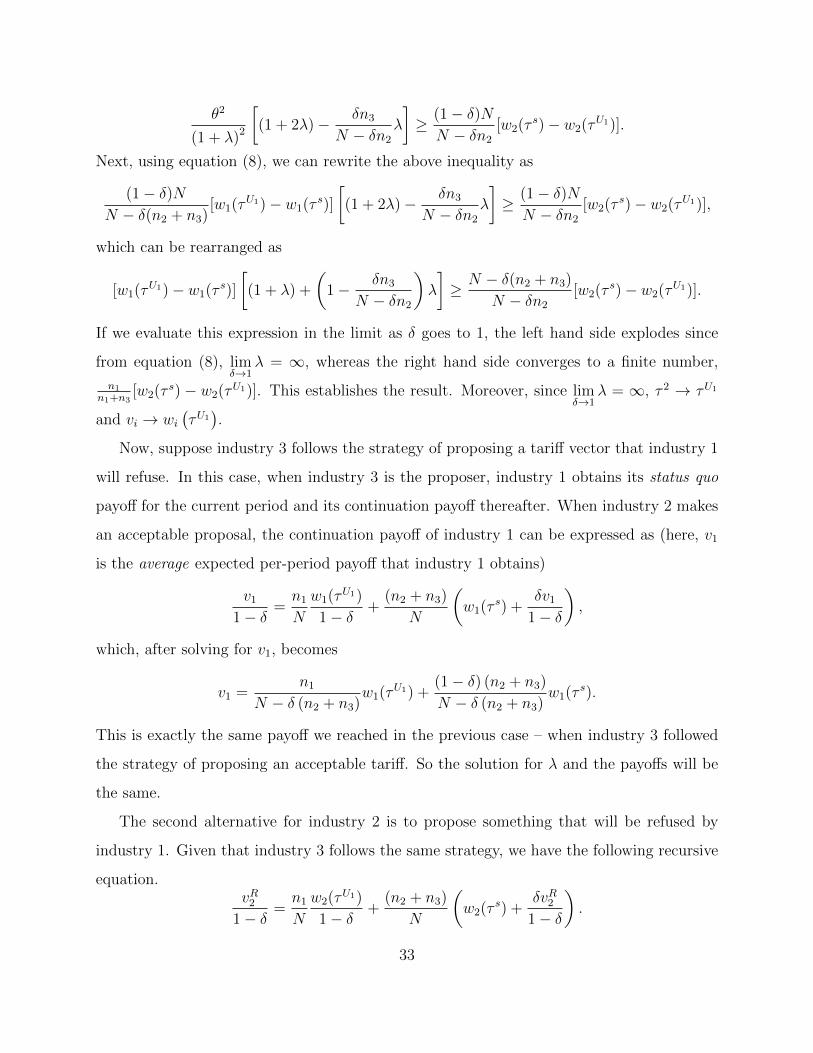
θ2

(1 + λ)2

[(1 + 2λ)− δn3

N − δn2

λ

]≥ (1− δ)N

N − δn2

[w2(τs)− w2(τ

U1)].

Next, using equation (8), we can rewrite the above inequality as

(1− δ)NN − δ(n2 + n3)

[w1(τU1)− w1(τ

s)]

[(1 + 2λ)− δn3

N − δn2

λ

]≥ (1− δ)N

N − δn2

[w2(τs)− w2(τ

U1)],

which can be rearranged as

[w1(τU1)− w1(τ

s)]

[(1 + λ) +

(1− δn3

N − δn2

)λ

]≥ N − δ(n2 + n3)

N − δn2

[w2(τs)− w2(τ

U1)].

If we evaluate this expression in the limit as δ goes to 1, the left hand side explodes since

from equation (8), limδ→1

λ = ∞, whereas the right hand side converges to a finite number,

n1

n1+n3[w2(τ

s) − w2(τU1)]. This establishes the result. Moreover, since lim

δ→1λ = ∞, τ 2 → τU1

and vi → wi(τU1).

Now, suppose industry 3 follows the strategy of proposing a tariff vector that industry 1

will refuse. In this case, when industry 3 is the proposer, industry 1 obtains its status quo

payoff for the current period and its continuation payoff thereafter. When industry 2 makes

an acceptable proposal, the continuation payoff of industry 1 can be expressed as (here, v1

is the average expected per-period payoff that industry 1 obtains)

v11− δ

=n1

N

w1(τU1)

1− δ+

(n2 + n3)

N

(w1(τ

s) +δv1

1− δ

),

which, after solving for v1, becomes

v1 =n1

N − δ (n2 + n3)w1(τ

U1) +(1− δ) (n2 + n3)

N − δ (n2 + n3)w1(τ

s).

This is exactly the same payoff we reached in the previous case – when industry 3 followed

the strategy of proposing an acceptable tariff. So the solution for λ and the payoffs will be

the same.

The second alternative for industry 2 is to propose something that will be refused by

industry 1. Given that industry 3 follows the same strategy, we have the following recursive

equation.vR2

1− δ=n1

N

w2(τU1)

1− δ+

(n2 + n3)

N

(w2(τ

s) +δvR2

1− δ

).

33

Solving for vR2 , we have

vR2 =n1

N − δ (n2 + n3)w2(τ

U1) +(1− δ) (n2 + n3)

N − δ (n2 + n3)w2(τ

s).

Comparing the payoffs associated with proposing a tariff vector that will be accepted and

proposing a tariff vector that will be rejected, we have

w2(τ21 , τ

22 , τ

23 ) ≥ (1− δ)w2(τ

s) + δvR2⇔

w2(τU1) + θ2(1+2λ)

(1+λ)2≥ (1− δ)w2(τ

s) + δn1

N−δ(n2+n3)w2(τ

U1) + δ(1−δ)(n2+n3)N−δ(n2+n3)

w2(τs), or

θ2

(1 + λ)2(1 + 2λ) ≥ (1− δ)N

N − δ (n2 + n3)

[w2(τ

s)− w2(τU1)]

.

As before, using equation (8), we can rewrite the above inequality as

(1− δ)NN − δ(n2 + n3)

[w1(τU1)− w1(τ

s)] (1 + 2λ) ≥ (1− δ)NN − δ (n2 + n3)

[w2(τ

s)− w2(τU1)]

,

which can be rearranged as

[w1(τU1)− w1(τ

s)] (1 + 2λ) ≥[w2(τ

s)− w2(τU1)]

.

Thus, the conclusion is the same. Since limδ→1

λ = ∞, the left-hand side goes to ∞, so

w2(τ2) > (1− δ)w2(τ

s) + δvR2 . Everything is symmetric for industry 3. So, independent of

the identity of the proposer, an agreement is always reached in the first period, τ 1 = τU1

while τ 2 → τU1 , τ 3 → τU1 , and vi → wi(τU1)

as δ → 1.

Proof of Proposition 2. When a legislator representing industry i is selected as the

proposer and chooses industry j 6= i as the coalition partner, we denote the chosen tariffs as

τ = (τ iji , τijj , τ

ijk ) where, τ iji is the tariff industry i gets, τ ijj is the tariff industry j gets and

τ ijk is the tariff industry k 6= i, j gets.

Now, suppose a legislator representing industry i is selected as the proposer and she

chooses industry j 6= i as the coalition partner. Her maximization problem is

maxτ iji ,τ

ijj ,τ

ijk

wi(τiji , τ

ijj , τ

ijk ) s.t. wj(τ

iji , τ

ijj , τ

ijk ) > (1− δ)wj(τ s) + δvj.

34

In the limit as δ → 1, the constraint can be rewritten as wj(τ) > vj. Hence, the maximization

problem becomes

maxτ

wi(τiji , τ

ijj , τ

ijk ) s.t. wj(τ

iji , τ

ijj , τ

ijk ) ≥ vj,

where (using equation (5))

wi(τi, τj, τk) = wi(τs) +

[θ(τi − τ si )− 1

2

∑l=i,j,k

[(τl +Ql)

2 − (τ sl +Ql)2]] ,

wj(τi, τj, τk) = wj(τs) +

[θ(τj − τ sj )− 1

2

∑l=i,j,k

[(τl +Ql)

2 − (τ sl +Ql)2]] .

The Lagrangian can be expressed as

L(τ iji , τijj , τ

ijk ) = wi(τ

iji , τ

ijj , τ

ijk ) + λij(wj(τ

iji , τ

ijj , τ

ijk )− vj),

where λij is the Lagrange multiplier when a legislator representing industry i is selected as

the proposer and she chooses industry j 6= i as the coalition partner. It represents the cost

to the proposing legislator of obtaining the additional votes needed to pass the proposal.

The first-order conditions, after simplification, are

τ iji =θ

1 + λij−Qi,

τ ijj =λijθ

1 + λij−Qj,

τ ijk = −Qk.

We first show that, in an SSPE in which all proposers employ mixed strategies in choosing

their coalition partners, the value of λij is independent of the identity of the proposer and of

the coalition partner, i.e., λij = λ for all i 6= j, i, j = 1, 2, 3. This follows from the following

two observations. First, a legislator would employ a mixed strategy in choosing a coalition

partner only when the ex post payoff her district enjoys is the same under each alternative.

In other words, when a legislator representing industry i is selected as the proposer, she

randomly picks an industry as a coalition partner if, for all i 6= j 6= k,

wi(τiji , τ

ijj , τ

ijk ) = wi(τ

iki , τ

ikj , τ

ikk )

35

⇔ θτ iji −1

2

∑l=i,j,k

[(τ ijl +Ql

)2 − (τ sl +Ql)2]

= θτ iki −1

2

∑l=i,j,k

[(τ ikl +Ql

)2 − (τ sl +Ql)2]

.

Using the equilibrium values of (τ iji , τijj , τ

ijk ) and (τ iki , τ

ikj , τ

ikk ), we have

θ2

1 + λij− 1

2

(

1 + (λij)2)θ2

(1 + λij)2

=θ2

1 + λik− 1

2

(

1 +(λik)2)

θ2

(1 + λik)2

.

It is easy to see that this is possible only if λij = λik. Second, when industry j is chosen

as a coalition partner, the ex post welfare it is offered would be independent of the identity

of the proposer, because whoever is the proposer always offers an ex post welfare of vj to

this industry, otherwise the proposal is rejected. Thus, for any i 6= j 6= k,

wj(τiji , τ

ijj , τ

ijk ) = wj(τ

kji , τ

kjj , τ

kjk )

⇔ θτ ijj −1

2

∑l=i,j,k

[(τ ijl +Ql

)2 − (τ sl +Ql)2]

= θτ kjj −1

2

∑l=i,j,k

[(τ kjl +Ql

)2− (τ sl +Ql)

2

].

Using the equilibrium values of (τ iji , τijj , τ

ijk ) and (τ kji , τ

kjj , τ

kjk ), we have

λijθ2

1 + λij− 1

2

(

1 + (λij)2)θ2

(1 + λij)2

=λkjθ2

1 + λkj− 1

2

(

1 +(λkj)2)

θ2

(1 + λkj)2

.

Again, this is possible only if λij = λkj. Together with the earlier observation, λij = λkj =

λik, which implies that λij = λ for all i 6= j, i, j = 1, 2, 3. Next, we find the equilibrium value

of λ in an SSPE in which all proposers employ mixed strategies in choosing their coalition

partners. We first write down the equilibrium ex post per capita welfare in three distinct

cases.

(i) when the districts that produce good j are selected as the proposer:

wproposerj = wj(τs) +

[θ2

1 + λ− θ(τ sj +Qj)−

1

2

((1 + λ2) θ2

(1 + λ)2−∑l=i,j,k

(τ sl +Ql)2

)].

(ii) when the districts that produce good j are selected as a coalition partner:

wpartnerj = wj(τs) +

[λθ2

1 + λ− θ(τ sj +Qj)−

1

2

((1 + λ2) θ2

(1 + λ)2−∑l=i,j,k

(τ sl +Ql)2

)].

36

(iii) when the districts that produce good j are left outside the coalition:

woutsidej = wj(τs) +

[−θ(τ sj +Qj)−

1

2

((1 + λ2) θ2

(1 + λ)2−∑l=i,j,k

(τ sl +Ql)2

)].

We next express the equilibrium continuation welfare of a district on a per capita basis.

To do so, we need to introduce randomization probabilities. Let sij denote the probability

that a legislator representing a district that produces good i chooses the districts producing

good j as a coalition partner. Then, vj can be expressed as

vj =njN

[sjiwproposerj + (1− sji)wproposerj ] +

niN

[sijwpartnerj + (1− sij)woutsidej ]

+nkN

[skjwpartnerj + (1− skj)woutsidej ]. (9)

After simplification, this becomes

vj = wj(τs) +

θ2

1 + λ

(njN

+(sijniN

+ skjnkN

)λ)

−θ(τ sj +Qj)−1

2

((1 + λ2) θ2

(1 + λ)2−∑l=i,j,k

(τ sl +Ql)2

). (10)

Next, observe that the maximization problem implies wpartnerj = vj (since the constraint

is binding in equilibrium). Hence, it must be true that

3∑j=1

wpartnerj =3∑j=1

vj.

Also note that

3∑j=1i 6=k 6=j

(sijniN

+ skjnkN

)=

(s12

n1

N+ s32

n3

N

)+(s13

n1

N+ s23

n2

N

)+(s21

n2

N+ s31

n3

N

)= (s12 + s13)

n1

N+ (s21 + s23)

n2

N+ (s31 + s32)

n3

N

=n1 + n2 + n3

N

= 1.

37

The condition3∑j=1

wpartnerj =3∑j=1

vj can now be expressed as

3λθ2

1 + λ− θ

3∑j=1

(τ sj +Qj

)− 3

2

((1 + λ2) θ2

(1 + λ)2−∑l=i,j,k

(τ sl +Ql)2

)

=θ2

1 + λ(1 + λ)− θ

3∑j=1

(τ sj +Qj

)− 3

2

((1 + λ2) θ2

(1 + λ)2−∑l=i,j,k

(τ sl +Ql)2

)

⇔ λ =1

2.

So, the value of λ can be determined without the knowledge of the randomization prob-

abilities. Plugging the equilibrium value of λ into the tariffs we found earlier gives

τ iji =2θ

3−Qi,

τ ijj =θ

3−Qj,

τ ijk = −Qk.

Plugging these into equation (5) gives the ex post per-capita payoffs stated in the proposition.

The final step of the proof is to show that there is an interior solution to all of the

randomization probabilities (this is what we assumed at the beginning of the proof). Since

the continuation per-period, per-capita welfare is equal to ex post welfare when chosen as a

coalition partner (by the maximization problem), i.e., vj = wpartnerj , we have

θ2

1 + λ

(njN

+(sijniN

+ skjnkN

)λ)

=λθ2

1 + λ

⇔ sijniN

+ skjnkN

= 1− 2njN

.

For simplicity, let s12 = s1, s23 = s2 and s31 = s3. Then,

s1n1

N+ (1− s3)

n3

N= 1− 2

n2

N,

s2n2

N+ (1− s1)

n1

N= 1− 2

n3

N,

s3n3

N+ (1− s2)

n2

N= 1− 2

n1

N.

38

Note that these equations are linearly dependent (two of them imply the third), so we

lose one degree of freedom. It is easy to check that, when n3

N≤ n2

N≤ n1

N≤ 1

2, there is an

interior solution in which si ∈ [0, 1] for all i. To see this, fix s3 and express s1 and s2 in

terms of s3:

s1 =1− 2n2

N− (1− s3)n3

Nn1

N

,

s2 = 1−1− 2n1

N− s3 n3

Nn2

N

.

Any value of s3 ∈[0,

1−2n1N

n3N

]yields s1, s2 ∈ [0, 1].

It is important to note that an industry may select its coalition partner with pure strategy.

However, there are limitations. Feasible solutions (i.e., the solutions that satisfy si ∈ [0, 1]

for all i) are

(s1, s2, s3) =

(1− 2n2

N− n3

Nn1

N

, 1−1− 2n1

Nn2

N

, 0

),

(s1, s2, s3) =

(1− n1

N− n2

Nn1

N

, 1,1− 2n1

Nn3

N

).

All three industries may use pure strategies only when n1

N= n2

N= n3

N= 1

3. In this case,

s1 = s2 = s3 in all SSPE, so (s1, s2, s3) = (1, 1, 1) and (s1, s2, s3) = (0, 0, 0) are both

possible. Similarly, when n1

N= 1

2, industries 2 and 3 may use pure strategies. In fact,

(s1, s2, s3) =(1− 2n2

N, 1, 0

)is the unique SSPE in this case. Other than these two special

cases, only industry 2 or industry 3 may select its coalition partner with pure strategy.

Finally, the continuation per-period welfare of a district on a per capita basis can be

expressed, for all j = 1, 2, 3, as

vj = wj(τs) +

[λθ2

1 + λ− θ

(τ sj +Qj

)− 1

2

((1 + λ2) θ2

(1 + λ)2−∑l=i,j,k

(τ sl +Ql)2

)]

= wj(τs) +

[θ

(θ

3−(τ sj +Qj

))−

59θ2 −

∑l=i,j,k (τ sl +Ql)

2

2

].

39

Proof of Proposition 3. We will prove payoff uniqueness by showing that the randomiza-

tion strategies that are not already accounted for in the proof of Proposition 2 cannot arise

in an SSPE. Possible scenarios include all three industries or only two industries using pure

strategies. We will eliminate all possibilities step by step. When only one industry uses pure

strategy, the proof of Proposition 2 is perfectly applicable, so possible SSPE involve industry

2 choosing industry 3 with pure strategy, or vice versa. All other possibilities can be ruled

out because they lead to non-interior solutions (i.e., si 6∈ [0, 1] for some i).

Before proceeding with the proof, we would like make an important observation that will

prove very helpful. The equilibrium per capita welfare function of the proposer,

wproposerj = wj(τs) +

[θ2

1 + λ− θ

(τ sj +Qj

)− 1

2

((1 + λ2) θ2

(1 + λ)2−∑l=i,j,k

(τ sl +Ql)2

)],

is strictly decreasing in λ for all λ > 0. This means that if λik > λkj, then we must have

sik = 0 because, otherwise, industry i can profitably deviate by mimicking industry k and

selecting industry j as a partner rather than industry k.

Observation 1. The following configuration cannot arise in an SSPE: sik = sjk = 1 for

i 6= j 6= k.

This is the case when one industry is selected as a coalition member with pure strategy

by each one of the other two industries. Intuitively, this puts industry k in a veto-player

position which enables it to achieve its first-best. This, in turn, leads to a profitable deviation

by each one of the other two industries. To see this, we follow the same steps as in the proof

of Proposition 2. Under the strategies sik = sjk = 1, both industry i and j give industry k

its continuation payoff, so,

λik = λjk.

For industry k to randomize between the other two industries according to ski ∈ [0, 1], it

must also be true that

λki = λkj.

40

Let λik = λjk = µ and λki = λkj = λ. Then, for industries i and j not to deviate from

sik = sjk = 1, we must have µ ≤ λ. The equilibrium ex post welfare of industry k as the

proposer and as a partner can be expressed as

wproposerk = wk(τs) +

[θ2

1 + λ− θ (τ sk +Qk)−

1

2

((1 + λ2) θ2

(1 + λ)2−∑l=i,j,k

(τ sl +Ql)2

)],

wpartnerk = wk(τs) +

[µθ2

1 + µ− θ (τ sk +Qk)−

1

2

((1 + µ2) θ2

(1 + µ)2−∑l=i,j,k

(τ sl +Ql)2

)].

By equation (9), then,

vk = wk(τs) +

nkNθ2

1 + λ+

(ni+nj)

Nµθ2

1 + µ− θ (τ sk +Qk)

−1

2

(nkN

(1 + λ2) θ2

(1 + λ)2+

(ni + nj)

N

(1 + µ2) θ2

(1 + µ)2−∑l=i,j,k

(τ sl +Ql)2

).

This leads, by the constraint wpartnerk = vk, to

µθ2

1 + µ− 1

2

((1 + µ2) θ2

(1 + µ)2

)=

nkNθ2

1 + λ+

(ni+nj)

Nµθ2

1 + µ− 1

2

(nkN

(1 + λ2) θ2

(1 + λ)2+

(ni + nj)

N

(1 + µ2) θ2

(1 + µ)2

)⇔ µθ2

1 + µ− 1

2

((1 + µ2) θ2

(1 + µ)2

)=

θ2

1 + λ− 1

2

((1 + λ2) θ2

(1 + λ)2

).

This is possible only when µ = 1/λ. Together with the earlier condition that µ ≤ λ, this

requires λ ≥ 1. Repeating the same steps for industry i, we have

wpartneri = wi(τs) +

[λθ2

1 + λ− θ (τ si +Qi)−

1

2

((1 + λ2) θ2

(1 + λ)2−∑l=i,j,k

(Ql + τ sl )2)]

,

vi = wi(τs) +

niNθ2

1 + µ+

nkNskiλθ

2

1 + λ− θ (τ si +Qi)

−1

2

((ni + nj)

N

(1 + µ2) θ2

(1 + µ)2+nkN

(1 + λ2) θ2

(1 + λ)2−∑l=i,j,k

(Ql + τ sl )2)

= wi(τs) +

(niN

+ nkNski)λθ2

1 + λ− θ (τ si +Qi)

−1

2

((ni + nj + nk)

N

(1 + λ2) θ2

(1 + λ)2−∑l=i,j,k

(Ql + τ sl )2)

,

41

where the last line uses the fact that µ = 1/λ. By the constraint wpartneri = vi, andni+nj+nk

N=

1, then,λθ2

1 + λ− 1

2

((1 + λ2) θ2

(1 + λ)2

)=

(niN

+ nkNski)λθ2

1 + λ− 1

2

((1 + λ2) θ2

(1 + λ)2

),

which can be satisfied only when λ = 0. Thus, we reach a contradiction.

Observation 2. Unless niN

=njN

= nkN

, the following configuration cannot arise in an

SSPE: sij = sjk = ski = 1 for i 6= j 6= k.

Under this configuration, each industry is selected as a coalition member by one of the

other two industries. As in the proof of Observation 1, for each industry to play according

to sij = sjk = ski = 1 and not to deviate to choosing another partner, we must have

λij ≤ λjk,

λjk ≤ λki,

λki ≤ λij.

These three inequalities can be satisfied only when λij = λjk = λki = λ.

Next, using equation (9), we express the continuation payoff of each industry as follows.

vi = wi(τs) +

[(niN

+ nkNλ)θ2

1 + λ− θ (τ si +Qi)−

1

2

((1 + λ2) θ2

(1 + λ)2−∑l=i,j,k

(Ql + τ sl )2)]

,

vj = wj(τs) +

[(njN

+ niNλ)θ2

1 + λ− θ

(τ sj +Qj

)− 1

2

((1 + λ2) θ2

(1 + λ)2−∑l=i,j,k

(Ql + τ sl )2)]

,

vk = wk(τs) +

[(nkN

+njNλ)θ2

1 + λ− θ (τ sk +Qk)−

1

2

((1 + λ2) θ2

(1 + λ)2−∑l=i,j,k

(Ql + τ sl )2)]

.

By the constraint wpartnerl = vl for each l = i, j, k, then,

λ =niN

+nkNλ,

λ =njN

+niNλ,

λ =nkN

+njNλ.

42

Summing each side and usingni+nj+nk

N= 1 gives

λ =1

2.

Plugging the value of λ into the above equations leads to

niN

+nkN

2=njN

+niN

2=nkN

+njN

2=

1

2.

But this is possible only when niN

=njN

= nkN

= 13.

Observation 3. The following configuration cannot arise in an SSPE: sij = sjk = 1

and ski ∈ (0, 1) for i 6= j 6= k.

Under this configuration, industry i is selected as a coalition member less often than the

others, which lowers its equilibrium continuation payoff. This, in turn, induces industry k to

choose industry i with pure strategy. Note that we have assumed ski ∈ (0, 1) since ski = 0

can be ruled out by Observation 1 while ski = 1 can be ruled out by Observation 2.

For each industry to play according to sij = sjk = 1 and ski ∈ (0, 1), we must have

λij ≤ λjk,

λjk ≤ λki,

λki = λkj,

λkj = λij.

These four expressions can again be satisfied only when λij = λjk = λki = λkj = λ.

Next, using equation (9), we express the continuation payoff of each industry:

vi = wi(τs) +

[(niN

+ nkNskiλ

)θ2

1 + λ− θ (τ si +Qi)−

1

2

((1 + λ2) θ2

(1 + λ)2−∑l=i,j,k

(Ql + τ sl )2)]

,

vj = wj(τs) +

[[njN

+(niN

+ nkNskj)λ]θ2

1 + λ− θ

(τ sj +Qj

)− 1

2

((1 + λ2) θ2

(1 + λ)2−∑l=i,j,k

(Ql + τ sl )2)]

,

vk = wk(τs) +

[(nkN

+njNλ)θ2

1 + λ− θ (τ sk +Qk)−

1

2

((1 + λ2) θ2

(1 + λ)2−∑l=i,j,k

(Ql + τ sl )2)]

.

43

By the constraint wpartnerl = vl for each l = i, j, k, then,

λ =niN

+nkNskiλ,

λ =njN

+(niN

+nkNskj

)λ,

λ =nkN

+njNλ.

Summing each side and usingni+nj+nk

N= 1 gives

λ =1

2.

Using λ = 12, ski =

1−2niN

nkN

from the first of the above equations. Plugging this expression

into the second equation and usingni+nj+nk

N= 1 gives

njN

+ 2niN

= 1.

However, the third equation above implies

2nkN

+njN

= 1,

so it must be that niN

=njN

= nkN

= 13. But then ski =

1−2niN

nkN

= 1, which is a contradiction.

Observation 4. Unless nkN

= 12, the following configuration cannot arise in an SSPE:

sij = sji = 1 and ski ∈ (0, 1) for i 6= j 6= k.

Under this configuration, industry k is never selected as a coalition member, which lowers

its equilibrium continuation payoff. This, in turn, leads to a deviation by the other two

industries. Note that we have assumed ski ∈ (0, 1) since both ski = 0 and ski = 1 can be

ruled out by Observation 1.

For each industry to play according to sij = sji = 1 and ski ∈ (0, 1), we must have

λki = λkj,

λki = λji,

λkj = λij.

44

Thus, λij = λji = λki = λkj = λ.

Next, using equation (9), we express the continuation payoff of industries i and j:

vi = wi(τs) +

[[niN

+(njN

+ nkNski)λ]θ2

1 + λ− θ (τ si +Qi)−

1

2

((1 + λ2) θ2

(1 + λ)2−∑l=i,j,k

(Ql + τ sl )2)]

,

vj = wj(τs) +

[[njN

+(niN

+ nkNskj)λ]θ2

1 + λ− θ(τ sj +Qj)−

1

2

((1 + λ2) θ2

(1 + λ)2−∑l=i,j,k

(Ql + τ sl )2)]

.

By the constraints wpartnerl = vl for l = i, j (note that wpartnerk = vk cannot be used here

since industry k is never selected as a coalition member), then,

λ =niN

+(njN

+nkNski

)λ,

λ =njN

+(niN

+nkNskj

)λ.

Summing each side and usingni+nj+nk

N= 1 gives

λ =ni + njN

.

Now, let us write down industry k’s continuation payoff:

vk = wk(τs) +

[nkNθ2

1 + λ− θ(τ sk +Qk)−

1

2

((1 + λ2) θ2

(1 + λ)2−∑l=i,j,k

(Ql + τ sl )2)]

.

But then, industry i (same applies for industry j, too) can deviate by selecting industry k

as a coalition partner and offering a tariff vector:(τ iki , τ

ikj , τ

ikk

)=

(θ

1 + nkN

−Qi,−Qj,nkNθ

1 + nkN

−Qk

),

in which case,

wproposeri = wi(τs) +

θ2

1 + nkN

− θ(τ si +Qi)−1

2

(

1 +(nkN

)2)θ2(

1 + nkN

)2 −∑l=i,j,k

(Ql + τ sl )2

wpartnerk = wk(τs) +

nkNθ2

1 + nkN

− θ(τ sk +Qk)−1

2

(

1 +(nkN

)2)θ2(

1 + nkN

)2 −∑l=i,j,k

(Ql + τ sl )2

.

45

Note that, unless nkN

= 12, we have nk

N< λ =

ni+njN

. Also note that(1+λ2)θ2

(1+λ)2is increasing

in λ for λ < 1. Hence, both industry i and k benefit. This is a contradiction to the initial

configuration.

References

[1] Anderson, K. and R.E. Baldwin, 1987. The political market for protection in industrial

countries. In: A.M. El-Agraa (ed.), Protection, Cooperation, Integration and Develop-

ment, MacMillan, New York.

[2] Baldwin, R.E., 1976. The political economy of postwar U.S. trade policy. The Bulletin,

No. 4, New York University Graduate School of Business Administration, New York.

[3] Baldwin, R.E., 1985. The Political Economy of U.S. Import Policy. Cambridge Univer-

sity Press, Cambridge, U.K.

[4] Baron, D.P., 1993. A theory of collective choice for government programs. Research

Paper No 1240, Stanford Graduate School of Business.

[5] Baron, D.P. and J.A. Ferejohn, 1989. Bargaining in legislatures. American Political

Science Review 83, pp. 1181-1206.

[6] Baron, D.P. and E. Kalai, 1993. The simplest equilibrium of a majority-rule division

game. Journal of Economic Theory 61, pp. 290-301.

[7] Battaglini, M. and S. Coate, 2007. Inefficiency in legislative policymaking: a dynamic

analysis. American Economic Review 97, pp. 118-149.

[8] Busch, M.L. and E. Reinhardt, 1999. Industrial location and protection: the political

and economic geography of U.S. nontariff barriers. American Journal of Political Science

43, pp. 1028-1050.

[9] Carson, J.L., G. Koger, M.J. Lebo and E. Young, 2010. The electoral costs of party

loyalty in Congress. American Journal of Political Science 54, pp. 598-616.

46

[10] Celik, L. and B. Karabay, 2011. A Note on Equilibrium Uniqueness in the Baron-

Ferejohn Model. Working Paper, CERGE-EI and University of Auckland, May. Avail-

able at SSRN: (http://ssrn.com/abstract=1718719).

[11] Celik, L., B. Karabay and J. McLaren, 2011. When is it optimal to delegate? The theory

of fast-track authority. Mimeo, CERGE-EI, University of Auckland and University of

Virginia.

[12] Eraslan, H., 2002. Uniqueness of stationary equilibrium payoffs in the Baron-Ferejohn

model. Journal of Economic Theory 103, pp. 11-30.

[13] Findlay, R. and S. Wellisz, 1982. Endogenous tariffs, the political economy of trade

restrictions, and welfare. In: J. Bhagwati (ed.), Import Competition and Response,

University of Chicago Press, Chicago.

[14] Fordham, B. and T. McKeown, 2003. Selection and influence: interest groups and con-

gressional voting on trade policy. International Organization 57, pp. 519-549.

[15] Fredriksson, P.G., X. Matschke and J. Minier, 2011. Trade policy in majoritarian sys-

tems: the case of the U.S. Canadian Journal of Economics 44, pp. 607-626.

[16] Gagnon, J.E., 2003. Long-run supply effects and the elasticities approach to trade.

International Finance Discussion Papers No 754, Board of Governors of the Federal

Reserve System (January).

[17] George, Henry, 1886. Protection or Free Trade. Reprinted 1949: Robert Schalkenbach

Foundation, New York.

[18] Grossman, G.M. and E. Helpman, 1994. Protection for sale. American Economic Review

84, pp. 833-850.

[19] Grossman, G.M. and E. Helpman, 2005. A protectionist bias in majoritarian politics.

Quarterly Journal of Economics 120, pp. 1239-1282.

47

[20] Hiscox, M., 2002. Commerce, coalitions, and factor mobility: evidence from congres-

sional votes on trade legislation. American Political Science Review 96, pp. 593–608.

[21] Irwin, D.A. and R.S. Kroszner, 1999. Interests, institutions, and ideology in securing

policy change: the Republican conversion to trade liberalization after Smoot-Hawley.

Journal of Law and Economics 42, pp. 643-673.

[22] Kalandrakis, A., 2004. A three-player dynamic majoritarian bargaining game. Journal

of Economic Theory 116, pp. 294-322.

[23] Karacaovali, B., 2011. Productivity matters for trade policy: theory and evidence. In-

ternational Economic Review 52, pp. 33-62.

[24] Ladewig, J., 2006. Domestic influences on international trade policy: factor mobility in

the United States, 1963-1992. International Organization 60, pp. 69–103.

[25] Lavergne, R.P., 1983. The political economy of U.S. tariffs: An empirical analysis.

Academic Press, New York.

[26] Lebo, M.J., A.J. McGlynn and G. Koger, 2007. Strategic party government: party

influence in Congress, 1789-2000. American Journal of Political Science 51, pp. 464–

481.

[27] Li, D., 2009. Multiplicity of equilibrium payoffs in three-player Baron-Ferejohn model.

Working paper, Chinese University of Hong Kong.

[28] Lindsay, J.M., 1990. Parochialism, policy, and constituency constraints: congressional

voting on strategic weapons systems. American Journal of Political Science 34, pp.

936-960.

[29] Magee, S., 1978. Three simple tests of the Stolper-Samuelson theorem. In: P. Oppen-

heimer (ed.), Issues in International Economics, Oriel Press, Stocksfield.

48

[30] Marquez, J., 1990. Bilateral trade elasticities. Review of Economics and Statistics 72,

pp. 70–77.

[31] Marvel, H.P. and E.J. Ray, 1983. The Kennedy round: evidence on the regulation of

international trade in the United States. American Economic Review 73, pp. 190-197.

[32] Mayer, W., 1984. Endogenous tariff formation. American Economic Review 74, pp.

970-985.

[33] McLaren, J. and B. Karabay, 2004. Trade policy making by an assembly. In: D. Mitra

and A. Panagariya (eds.), The Political Economy of Trade, Aid and Foreign Investment

Policies: Essays in Honor of Edward Tower, Elsevier, Amsterdam.

[34] Nelson, D.R., 1999. The political economy of trade policy reform: social complexity and

methodological pluralism. Journal of International Trade and Economic Development

8, pp. 3–26.

[35] Nelson, D.R., 2007. The political economy of protection: a short survey. Working paper,

Tulane University.

[36] Osborne, M.J. and A. Rubinstein, 1994. A Course in Game Theory. MIT Press, Cam-

bridge, MA.

[37] Primo, D.M., 2006. Stop us before we spend again: institutional constraints on govern-

ment spending. Economics and Politics 18, pp. 269–312.

[38] Ray, E.J., 1981. The determinants of tariff and nontariff trade restrictions in the United

States. Journal of Political Economy 89, pp. 105-121.

[39] Ray, E.J. and H.P. Marvel, 1984. The pattern of protection in the industrialized world.

Review of Economics and Statistics 66, pp. 452-458.

[40] Riker, W.H., 1962. The Theory of Political Coalitions. Yale University Press, New

Haven.

49

[41] Rodrik, D., 1995. Political economy of trade policy. In: G.M. Grossman and K. Rogoff

(eds.), Handbook of International Economics, Volume 3, Chapter 28, Elsevier, Amster-

dam.

[42] Tarbell, I.M., 1911. The Tariff in Our Times. MacMillan, New York.

[43] Willmann G., 2004. Why legislators are protectionists: the role of majoritarian voting

in setting tariffs. http://www.ssrn.com/abstract=564587.

50