trades: a new software to derive orbital parameters from

Astronomy & Astrophysics manuscript no. LucaBorsato_trades01_AA201424080 c©ESO 2021June 29, 2021

TRADES: A new software to derive orbital parameters fromobserved transit times and radial velocities

Revisiting Kepler-11 and Kepler-9

L. Borsato1, 2, F. Marzari1, V. Nascimbeni1, 2, G. Piotto1, 2, V. Granata1, 2, L. R. Bedin2, and L. Malavolta1, 2

1 Department of Physics and Astronomy, Università degli Studi di Padova, Via Marzolo, 8 I-35131 Padovae-mail: [email protected]

2 INAF – Osservatorio Astronomico di Padova, vicolo dell’Osservatorio 5, 35122 Padova, Italy

Received 28 April, 2014 / Accepted 7 August, 2014

ABSTRACT

Aims. With the purpose of determining the orbital parameters of exoplanetary systems from observational data, we have developeda software, named TRADES (TRAnsits and Dynamics of Exoplanetary Systems), to simultaneously fit observed radial velocities andtransit times data.Methods. We implemented a dynamical simulator for N-body systems, which also fits the available data during the orbital integrationand determines the best combination of the orbital parameters using grid search, χ2 minimization, genetic algorithms, particle swarmoptimization, and bootstrap analysis.Results. To validate TRADES, we tested the code on a synthetic three-body system and on two real systems discovered by the Keplermission: Kepler-9 and Kepler-11. These systems are good benchmarks to test multiple exoplanet systems showing transit time vari-ations (TTVs) due to the gravitational interaction among planets. We have found that orbital parameters of Kepler-11 planets agreewell with the values proposed in the discovery paper and with a a recent work from the same authors. We analyzed the first threequarters of Kepler-9 system and found parameters in partial agreement with discovery paper. Analyzing transit times (T0s), covering12 quarters of Kepler data, that we have found a new best-fit solution. This solution outputs masses that are about 55% of the valuesproposed in the discovery paper; this leads to a reduced semi-amplitude of the radial velocities of about 12.80 ms−1.

Key words. methods: numerical – celestial mechanics – stars: planetary systems – stars: individual: Kepler-11 – stars: individual:Kepler-9

1. Introduction

Now, more than 1779 planets1 have been discovered and con-firmed in about 1102 planetary systems. Around 460 planetarysystems are known to be multiple planet systems. Hundreds ofKepler planetary candidates with multiple transit-like signals arestill waiting confirmation (see Latham et al. 2011; Lissauer et al.2011b). The usual way to characterize multiple planet systemsis by combining information from both transits and radial ve-locities (RVs). An effect due to the presence of multiple planetsis the transit time variation (TTV): the gravitational interactionbetween two planets causes a deviation from the Keplerian orbitand, as a consequence, the transit times (T0s) of a planet maybe not strictly periodic (see Agol et al. 2005; Holman & Murray2005; Miralda-Escudé 2002). This effect can be also exploited toinfer the presence of an unknown planet, even if it does not tran-sit the host star (Agol et al. 2005; Holman & Murray 2005). Forexample, the Kepler Transit Timing Observations series (TTO,Ford et al. 2011, and references therein) and TASTE project(Nascimbeni et al. 2011, and references therein) demonstrate theuse of this technique.

The problem of determining the masses and the orbital pa-rameters of the planets in a multiple system is a difficult in-verse problem. In some works, the authors adopted an analytic

1 http://exoplanet.eu/catalog, 2014 March 21st.

approach to the problem (e.g., Nesvorný & Morbidelli 2008;Nesvorný 2009), developing a method from the perturbation the-ory (Hori 1966; Deprit 1969), where the T0s are computed as aFourier series. A drawback of this method is that it does not takeinto account for the so-called mean motion resonance (MMR) orcases that are just outside the MMR. We have a MMR when theratio of the periods of two planets is a multiple of a small inte-ger number, such as 2:1. Two planets reciprocally in MMR, orjust outside it, show a strong TTV signal that is easily detectableeven with ground-base facilities.The method described in this paper is based on a direct numer-ical N-body approach (Steffen & Agol 2005; Agol & Steffen2007), which is conceptually simpler, but computationally inten-sive. Very recently, Deck et al. (2014) have developed TTVFast,a symplectic integrator that computes transit times and radial ve-locities of an exoplanetary system.An example of the application based on the TTV technique canbe found in Nesvorný et al. (2013), where the authors have pre-dicted the presence of the planet KOI-142c in the system, whichhas been recently confirmed by Barros et al. (2013).

In Sect. 2 we introduce the TRADES program, the basic for-mulas, and methods to calculate radial velocities and transittimes; in Sects. 3, 4, and 5, we run TRADES on a synthetic 3-bodysystem, Kepler-11, and Kepler-9, respectively. We summarizeand discuss the results in the Sect. 6.

Article number, page 1 of 14

arX

iv:1

408.

2844

v2 [

astr

o-ph

.EP]

30

Sep

2014

http://exoplanet.eu/catalog/

A&A proofs: manuscript no. LucaBorsato_trades01_AA201424080

2. TRADES

We have developed a computer program (in Fortran 90 andopenMP) for determining the possible physical and dynamicalconfigurations of extra-solar planetary systems from observa-tional data, known as TRADES, which stands for TRAnsits andDynamics of Exoplanetary Systems. The program TRADESmod-els the dynamics of multiple planet systems and reproduces theobserved transit times (T0, or mid-transit times) and radial ve-locities (RVs). These T0s and RVs are computed during the inte-gration of the planetary orbits. We have developed TRADES fromzero because we want to avoid black-box programs,it would beeasier to parallelize it with openMP, and include additional algo-rithms.

To solve the inverse problem, TRADES can be run in four dif-ferent modes: 1) ‘grid’ search, 2) Levenberg-Marquardt2 (LM) al-gorithm, 3) genetic algorithm (GA, we used the implementationnamed PIKAIA3, Charbonneau 1995), 4) and particle swarm op-timization (PSO4, Tada 2007). In each mode, TRADES comparesobserved transit times (T0,obss) and radial velocities (RVobss)with the simulated ones (T0,sims and RVsims).

1. In the grid search method, TRADES samples the orbital ele-ments of a perturbing body in a four-dimensional grid: themass, M, the period, P (or the semi-major axis, a), the ec-centricity, e, and the argument of the pericenter, ω. The gridparameters can be evenly sampled on a fixed grid by settingthe number of steps, or the step size, or by a number of pointschosen randomly within the parameter bounds. For any givenset of values, the orbits are integrated, and the residuals be-tween the observed and computed T0s and RVs are com-puted. For each combination of the parameters, the LM al-gorithm can be called and the best case is the one with thelowest residuals (lowest χ2). We have selected these four pa-rameters for the grid search because they represent the min-imal set of parameters required to model a coplanar system.In the future, we intend to add the possibility of making thegrid search over all the set of parameters for each body.

2. After an initial guess on the orbital parameters of the per-turber, which could be provided by the previously describedgrid approach, the LM algorithm exploits the Levenberg-Marquardt minimization method to find the solution withthe lowest residuals. The LM algorithm requires the analyticderivative of the model with respect to the parameters to befitted. Since the T0s are determined by an iterative methodand the radial velocities are computed using the numericalintegrator, we cannot express these as analytic functions offitting parameters. We have adopted the method described inMoré et al. (1980) to compute the Jacobian matrix, whichis determined by a forward-difference approximation. Theepsfcn parameter, which is the parameter that determinesthe first Jacobian matrix, is automatically selected in a log-arithmic range from the machine precision up to 10−6; thebest value is the one that returns the lower χ2. This methodhas the advantage to be scale invariant, but it assumes thateach parameter is varied by the same epsfcn value (e.g., avariation of 10% of the period has a different effect than avariation of the same percentage of the argument of pericen-ter).

2 lmdif converted to Fortran 90 by Alan Miller(http://jblevins.org/mirror/amiller/) from MINPACK.3 PIKAIA (http://www.hao.ucar.edu/modeling/pikaia/pikaia.php) con-verted to Fortran 90 by Alan Miller.4 based on the public Fortran 90 code athttp://www.nda.ac.jp/cc/users/tada/

3. The GA mode searches for the best orbit by performing agenetic optimization (e.g. Holland 1975; Goldberg 1989),where the fitness parameter is set to the inverse of the χ2.This algorithm is inspired by natural selection which is thebiological process of evolution. Each generation is a newpopulation of ‘offspring’ orbital configurations, that are theresult of ‘parent’ pairs of orbital configurations that areranked following the fitness parameter. A drawback of theGA is the slowness of the algorithm, when compared to otheroptimizers. However, the GA should converge to a global so-lution (if it exists) after the appropriate number of iterations.

4. The PSO is another optimization algorithm that searches forthe global solution of the problem; this approach is inspiredby the social behavior of bird flock and fish school (e.g.,Kennedy & Eberhart 1995; Eberhart 2007). The fitness pa-rameter used is the same as the GA, the inverse of the χ2. Foreach ‘particle’, the next step (or iteration) in the space of thefitted parameters is mainly given by the combination of threeterms: random walk, best ‘particle’ position (combination ofparameters), and best ‘global’ position (best orbital configu-ration of the all particles and all iterations).

The grid search is a good approach in case that we want toexplore a limited subset of the parameter space or if we want toanalyze the behavior of the system by varying some parameters,for example to test the effects of a growing mass for the perturb-ing planet. GA and PSO are good methods to be used in case of awider space of parameters. The orbital solution determined withthe GA or the PSOmethod is eventually refined with the LMmode.

For each mode, TRADES can perform a bootstrap analysis tocalculate the interval of confidence of the best-fit parameter set.We generate a set of T0s and RVs from the fitted parameters,and we add a Gaussian noise having the calculated value (of T0sand RVs) as the mean and the corresponding measurement er-ror as variance. We fit each new set of observables with the LM.We iterate the whole process thousands of times to analyze thedistribution for each fitted parameter.

2.1. Orientation of the reference frame

For the transit time determination, the propagation of the trajec-tories of all planets in the system is performed in a referenceframe with the Z-axis pointing to the observer, while the X-Yplane is the sky plane. At a given reference epoch, the Keple-rian orbital elements of each planet are: period P (or semi-majoraxis a), inclination i, eccentricity e, argument of the pericenterω, longitude of the ascending node Ω, and time of the passage atthe pericenter τ (or the mean anomaly M). Given the orbital ele-ments we first compute the initial radius r and velocity r vectorsin the orbital plane (e.g., see Murray & Dermott 2000):

r =

xyz

=

a (cos E − e)a√

1 − e2 sin E0

, (1)

r =

xyz

=

n

1−e cos E (−a sin E)n

1−e cos E

(a√

1 − e2 cos E)

0

, (2)

where n = 2π/P is the mean motion, E is the eccentricanomaly obtained from the solution of the Kepler’s equation,M = E − e sin E, with the Newton-Raphson method (e.g., seeDanby 1988; Murray & Dermott 2000; Murray & Correia 2011).


http://jblevins.org/mirror/amiller/


http://www.hao.ucar.edu/modeling/pikaia/pikaia.php


http://www.nda.ac.jp/cc/users/tada/

L. Borsato et al.: TRADES: a new software to derive orbital parameters

Then, we rotate the state vector by applying three consecutive ro-tation matrices, Rl(φ) (e.g., see Danby 1988; Murray & Dermott2000; Murray & Correia 2011) where φ is the rotation angle andl is the rotation axis (where l is 1, 2, 3 for x′, y′, z′). To rotatethe initial state vector from the orbital plane to the observer ref-erence frame, we have to use the transpose of the rotation matrix,RT

l (φ) with angles ω, i, and Ω. After this rotation, the X-Y planeis the sky plane with the Z-axis pointing to the observer, and wedetermine the initial state vector of each k-th planet: X

YZ

= RT3 (Ω) RT

1 (i) RT3 (ω)

xyz

. (3)

The same rotations have to be applied to the initial velocity vec-tor. The inclinations are measured from the sky-plane. Indeed,a planet with inclination of 0 has an orbit that lies on the sky-plane (X-Y plane), that is, it is seen face-on. The orbit of a planetwith i = 90 is seen edge-on (it transits exactly through the cen-ter of the star), and it lies on the X-Z plane. From the initialstate vector, TRADES integrates the astrocentric equation of mo-tion (e.g. Murray & Dermott 2000; Fabrycky 2011) of planet k:

rk = −G (M1 + Mk)rk

r3k

+ GN∑

j=2; j,k

M j

r j − rk

|r j − rk |3 −

r j

r3j

, (4)

where M1 is the mass of the star and N the number of bodies; thefirst term is the direct gravitational force, and the second term isthe indirect force due to mutual interaction of the planets. Theorbits are computed with the Runge-Kutta-Cash-Karp integrator(RKCK, Cash & Karp 1990; Press et al. 1996). It is not a sym-plectic integrator5, and it is not well suited for long–term timeintegrations. Instead, it uses small and variable steps (it self ad-justs the step-size to maintain the numerical precision during thecomputation of the orbits), is fast, and preserves the total energyand the total angular momentum during the time scales of oursimulations.

2.2. Transit determination

We chose the change of sign of the X or Y coordinates betweentwo consecutive steps of each planet trajectory as first conditionof an eclipse. When this condition is met, following Fabrycky(2011, chap. 2.5), we have to seek roots of the sky-projectedseparation rs,k ≡ (Xk,Yk) with the Newton-Raphson method bysolving

g(Xk, Xk,Yk, Yk) = rs,k · rs,k = XkXk + YkYk = 0 (5)

then moving and iterating by the quantity,

δt = −g

(∂g

∂t

)−1

. (6)

In this way, we can determine with high precision the mid-transittime and the corresponding state vector (rmid, rmid) with an accu-racy equal to the selected δt. We decided to set this accuracy inTRADES at the machine precision, which can be fine-tuned in thesource of the code and defines the type of the chosen variables.

Then, we determine if we have four contact times, or justtwo (in the case of a grazing eclipse), or no transit, comparing

5 A symplectic integrator has been designed to numerically solve theHamilton’s equation by preserving the Poincaré invariants.

the module of the sky-projected separation at the transit time,|rs,mid|, with the radius of the star, R?, and of the planets, Rk, asin Fabrycky (2011). If the transit (or the occultation) does exist,we move about ∓R?/|rs,mid| from the tmid backward (−) for firstand second contact, and forward (+) for third and fourth contact.Then, we solve

h(Xk,Yk) = X2k + XkXk + Y2

k + YkYk = 0 (7)

and move of

δt = −h(∂h∂t

)−1

(8)

until δt is less than the accuracy found (the same adopted in find-ing the transit time).

We based our approach on Fabrycky (2011), but we used abisection-Newton-Raphson hybrid method, which is guaranteedto be bound near the solution, and we assume that the orbital ele-ments of the bodies are almost constant around the center of thetransit. Because of the latter assumption, we use F(ti, ti−1) andG(ti, ti−1) functions (called f (t, t0) and g(t, t0) in Danby 1988;Murray & Dermott 2000) to compute the planetary state vectorsinstead of the integrator while seeking the transit times:

ri(t) = F(ti, ti−1)ri−1 + G(ti, ti−1)ri−1ri(t) = F(ti, ti−1)ri−1 + G(ti, ti−1)ri−1

(9)

whereri−1 = r(ti−1)ri−1 = r(ti−1) (10)

withF(ti, ti−1) = ai

ri−1[cos(Ei − Ei−1) − 1] + 1

G(ti, ti−1) = (ti − ti−1) + 1ni

[sin(Ei − Ei−1) − (Ei − Ei−1)]

(11)

and F(ti, ti−1) = −a2

iriri−1

ni sin(Ei − Ei−1)G(ti, ti−1) = ai

ri[cos(Ei − Ei−1) − 1] + 1

. (12)

where ti = ti−1 + δti−1 at the i-th iterations; Ei and Ei−1 are theeccentric anomalies at the i-th and i-th−1 iterations. This allowsthe code to run faster than using the integrator, which has a lowernumber of function calls, to seek the transit and contact times.

The light coming from the star is delayed due to the motionof the star around the barycenter of the system (Irwin 1952),and so TRADES corrects for the light-time travel effect (LTE= −Zbarycentric

? /c, see Fabrycky 2011), each contact, and centertransit time.

2.3. RV calculation and other constraints

For each observed RV (when available), TRADES integrates theorbits of the planets to the instant of the RV point and calculatesthe RV as the opposite of the z-component of the barycentricvelocity of the star (rvsim = −Zbarycentric

? in the right unit of mea-surement). The observed RV is defined as RVobs = γ + rvobs,where γ is the motion of the barycenter of the system and rvobsis the reflex motion of the star induced by the planets. The pro-gram TRADES calculates γsim as the weighted mean of the differ-ence ∆rv j = RV j,obs − rv j,sim with j from one to the number of



RVs. The final simulated RV is RV j,sim = γsim + rv j,sim. We areplanning to implement the γsim fitting rather than the describedweighted mean method.

Furthermore, we added some constraints on the orbit duringthe integration, setting a minimum and a maximum semi-major-axis for the system, amin and amax, respectively. The lower limithas been set equal to the star radius, while the maximum limithas been set equal to five times the largest semi-major axis ofthe system calculated from the periods of the planets. In the GA,we have used the largest period boundary. We use the definitionof the Hill’s sphere to obtain minimum distance allowed betweentwo planets (Murray & Dermott 2000). In this case, when theseconstraints are not be respected, the integration is stopped, andthe χ2 returned is set to the maximum value allowed by the com-piler, so the combination of the parameters is rejected.

3. Validation with simulated system

To validate TRADES, we simulated a synthetic system with twoplanets having known orbital parameters. We chose a star witha mass and radius equal to the Sun, a first planet named b withJupiter mass and radius (MJup and RJup), and a second planetnamed c with mass and radius of Saturn (MSat and RSat). Weassumed a co-planar system with inclination of 90 (perfectlyedge-on). The input orbital elements of the system are summa-rized in Table 1.

Table 1. Parameters of the simulated system in section 3.

Parameter Star Planet b Planet cM 1. M 1. MJup 1. MSatR 1. R 1. RJup 1. RSata 0.1 AU 0.2 AUe 0.1 0.3ω 90 90M 0 0i 90 90Ω 0 0

We simulated the system with TRADES for 500 days. Wecomputed all T0s for each body and we call these times the ‘true’transit times (T0,trues) of the system. Then, we created sets of syn-thetic transit times (T0,synths), such as

T0,synth = T0,true + N(0, 1) ×P3× s , (13)

where s is a scaling factor varying from 0.01 to 1.5 (on twentylogarithmic steps) needed to simulate good to very bad measure-ment cases; N(0, 1) is Gaussian noise with 0 as mean and 1 asvariance. The P/3 factor is needed to scale the Gaussian noisein the right unit of time, and avoids confusion between transitsand occultations at the same time. Furthermore, for each set ofT0,synths, we selected a random number of transits (at least N/3with N being the total number of transits of each planet) to sim-ulate observed transits.

We fixed the orbital parameters of planet b, and we fitted M,P, e, ω, M, and Ω of planet c. We ran TRADES in LM mode foreach scaling factor, and we calculated the difference of the pa-rameters (∆) as the determined parameters minus the input pa-rameters. We repeated the simulation ten times (we calculatednew Gaussian noise and the number of observed times everytime). In Fig. 1, we plotted then mean and median of ten sim-ulations for each s scaling factor value. The parameters of the

Δ median Δ mean

ΔPc [m

in]

-50.0-25.0

0.025.050.0

Δec

0.000

0.025

0.050

Δωc [๐ ]

-25.0

0.0

25.0

ΔMc [๐ ]

-10.0

0.0

10.0

ΔΩc [๐ ]

-40.0

-20.0

0.0

20.0

s × P/3 [days]0.1 1.0 10.0

Fig. 1. Mean (red-open circles with 1σ error bars) and median (blue-filled circles) variation (∆) of fitted parameters of planet c for each valueof the measurement errors on T0, which are here parametrized as s×P/3(see text for details).

system derived by TRADES depart from the ‘true’ values only forextremely large measurement errors.

To further test the robustness of the algorithm, we took theT0,trues (without added noise) and varied the initial semi-majoraxis of planet c from 0.19 AU to 0.21 AU with the TRADESgrid+LM mode by fitting the same parameters of the previoustest. The algorithm nicely converged to the values from whichthe synthetic data were generated, except for initial parametersthat are too far from the right solution. This is due to the knownlimitation of the LM algorithm, which converges to close localminima from an initial set of parameters. Figure 2 shows thevariation of the parameter differences (∆) as function of the ini-tial semi-major axis. This test shows how well TRADES recoversthe parameters in the case of a bad guess of the initial parame-ters.

We measured the computational time required by TRADES,and we found that it can integrate (initial step size of 0.0001day) a 3-body synthetic system for 3000 days writing the or-bits, the Keplerian elements, and the constants of motion for each0.1 days in about 2.3 seconds. An integration of 1000 days hasbeen performed in less than 1 second and in less than half secondfor 500 days of integration time, but most of the time have beenspent writing files. We want to stress that TRADES write thesefiles only at the end of the simulations, so the real computationis faster than these estimates. The time required by TRADES tocomplete the grid search was about 51 minutes with 10 proces-sors of an Intelr Xeonr CPU E5-2680 based workstation. Foreach combination of the initial parameters in the grid search,TRADES runs 10 times the LM to select the best value for the pa-rameter epsfcn, that is needed to construct the initial Jacobian.

We tested the PSO+LM algorithm by fitting the same param-eters of the grid search with limited boundaries except for thesemi-major axis of planet c, for which we used the same limitof the grid search (ac = [0.19, 0.21] AU). We ran this test four



Δ[χ2r < 10] Δ[χ2

r > 10]

ΔM [M

Jup]

-1.5-1.0-0.50.0

ΔP [m

in]

−5000−2500

02500

Δe

-0.500-0.2500.0000.250

Δω [๐ ]

-100.0

0.0

100.0

ΔM [๐ ]

-100.0

0.0

100.0

ΔΩ [๐ ]

-100.0

0.0

100.0

a [au]0.190 0.192 0.194 0.196 0.198 0.200 0.202 0.204 0.206 0.208 0.210

Fig. 2. Variations (∆) of the fitted parameters for different initial val-ues of the semi-major axis of the planet c; each point corresponds to adifferent simulation. In this case, the input parameters (of planet c) arethe parameters in Table 1 used to generate the exact transit times. Thegoodness of the fit has been color-coded so that good fits (χ2

r < 10) havebeen plotted as blue points and bad fits (χ2

r > 10) as open circles. Thesmall gaps are due to the random sampling used to generate the grid inthe semi-major axis a.

times with 200 particles for 2000 iterations, and TRADES alwaysreturned the right parameter values in less than about 1 hour and40 minutes with 10 processors.

4. Test case: Kepler-11 system

The system Kepler-11 (KOI-157, Lissauer et al. 2011a) has sixtransiting planets packed in less than 0.5 AU, making a complexand challenging case to be tested with TRADES.From the spectroscopic analysis of HIRES high-resolution spec-tra, Lissauer et al. (2011a) derived the stellar parameters (effec-tive temperature, surface gravity, metallicity, and projected stel-lar equatorial rotation) and determined the mass and the radiusof Kepler-11 star to be 0.95 ± 0.10 M and 1.1 ± 0.1 R.

We first performed an analysis of the Kepler-11 system onlyon the data from the first three quarters of Kepler observationspublished by Lissauer et al. (2011a) and supplementary informa-tion (SI). We used the first circular model from the Lissauer et al.(2011a, SI) as an initial guess, which fixed the eccentricity andthe longitude of the ascending node to zero for all the planets;hereafter we call this model Lis2011 (see first column in Table 2for a summary of the orbital parameters). We used this modelbecause the authors did not provide any information about themean anomalies (or the time of the passage at the pericenter) forthose planets. In this case, the argument of the pericenter, ω, isundetermined, so we fixed it to ω = 90 for each planet. We thencalculated the initial mean anomaly, M0 at the reference epochtepoch = 2 455 190.0 (BJDUTC

6 ), setting the transit time (T0, Lis-

6 In the FITS header of Kepler data the time standard is reported asBarycentric Julian Day in Barycentric Dynamical Time (BJDTDB), but

Sky-Plane

Y [A

U]

-0.005

0.000

0.005

X [AU]-0.005 0.000 0.005

RV model

RV

[m/s

]

-5.000

0.000

5.000

BJD - 2455190.000-250.000 0.000 250.000

planet bplanet cplanet dplanet eplanet fplanet g

Face-on Projection

Z [A

U]

-0.500

0.000

0.500

X [AU]-0.500 0.000 0.500

Fig. 3. Orbits of the Kepler-11 system with initial parameters fromLis2011 model (circular model, see Table 2). The planet marker sizeis scaled with the mass of the planet. Top-right: ‘Sky Plane’, Kepler-11 system as seen from the Kepler satellite; we plotted only one orbitnear a transit for each planet. Each circle is the position of a planet ata given integration time step. Bottom-right: Projection of the system asseen face on. The big markers are the initial points of the integration.Bottom-left: RV model from the simulation.

sauer et al. 2011a, SI Table S4) as the time of passage at thepericenter:

M0 = n · (tepoch − T0) , (14)

where n is the mean motion of the planet.Lissauer et al. (2011a) gave an upper limit of 300 M⊕ on the

mass of the planet Kepler-11g, while they set it to zero in thethree dynamical models of the supplementary information , andwe followed the same approach. Figure 3 shows the orbits andRVs of the Kepler-11 planets, according to the Lis2011 model.

We fitted a linear ephemeris (Table 3) to the observed transittimes of each planet for the first three quarters and computed theObserved−Calculated (O − C) diagrams, where O is T0,obss andC is the transit time calculated from the linear ephemeris.

We ran TRADES and fitted masses, periods, and mean anoma-lies of each planet. Hereafter, the orbital solution we have de-termined with TRADES is named with a short ID of the system(K11 for Kepler-11 and K9 for Kepler-9) and a Roman number(K11-I, K11-II, and so on). See solution K11-I in Table 2 for asummary of the parameters determined with TRADES (with 2σconfidence intervals from bootstrap analysis), which agree withthose published by Lissauer et al. (2011a). For each bootstraprun, we run 1000 iterations to obtain the confidence intervals atthe 97.72 percentile (2σ) of the distribution of each parameter.We calculated the residuals as the difference between the ob-served and simulated T0s. The residuals after the TRADES-LM fitare smaller than those with simulated transit times, that obtainedwith original parameters, and the final χ2

r is around ≈ 1.25 for

it is specified in the KSCI-19059 Subsect. 3.4 that the correct time isBarycentric Julian Day in Coordinated Universal Time (BJDUTC).



88 degrees of freedom (dof, calculated as the difference betweenthe number of data and the number of fitted parameters).

We also used the same initial conditions of solution K11-I,but this time we fitted the eccentricity and the argument of peri-center of all the planets. In this case, the LM did not move fromthe initial conditions even if it properly ended the simulationand returned reasonable errors. In the user guide of MINPACK(Moré et al. 1980), the user is warned to carefully analyze thecase in which one has a null initial parameter. We set the initialeccentricities to a small but non-zero value of 0.0001. This smallchange was able to let the LM algorithm to properly return rea-sonable parameter values; see solution K11-II in Table 2 for asummary of the parameters.

The resulting masses of the solutions K11-I and K11-II allagree within 2σ with the discovery paper (Lissauer et al. 2011a)and with all the best-fit solutions determined by Migaszewskiet al. (2012). In the latter work, the authors presented differ-ent sets of orbital parameters determined with an approach sim-ilar to ours (direct N-body simulation with genetic algorithm,Levenberg-Marquardt, and bootstrap), but they directly fit theflux of Kepler light curves (so-called dynamical photometricmodel) without fitting the transit times.

4.1. Transit time analysis of the twelve quarters

Recently, Lissauer et al. (2013) analyzed the transit times cov-ering fourteen quarters of Kepler data (in long and short ca-dence mode). A new independent extraction of T0s from the lightcurves made by Lissauer et al. (2013, hereafter we call the dy-namical model from this work Lis2013, see column five of Ta-ble 2) led the authors to change the value of some parameters ofthe system. For example, they determined a mass of 2.9+2.9

−1.6 M⊕of the planet c that is lower than 15.82 ± 2.21 M⊕ published inthe discovery paper (Lissauer et al. 2011a). Unfortunately the au-thors have not published the T0, so we used the data from Mazehet al. (2013) that recently published the transit times for twelvequarters of the Kepler mission for 721 KOIs.

We used the linear ephemeris by Lissauer et al. (2013) tocompute the O − Cs for the T0s from Mazeh et al. (2013). Wefound a remarkable mismatch with the O−Cs plotted in the paperby Lissauer et al. (2013). We stress that the T0s by Mazeh et al.(2013) are calculated with an automated algorithm. It would beadvisable to more carefully analyze the light curves determiningthe T0s with higher precision, but it is not the purpose of thiswork. We analyzed the system with all transit times from Mazehet al. (2013) without any selection, and they lead to unphysicalresults. We then decided to discard data with duration and depthof the transits that are 5σ away from the median values. Thisselection defines the sample of T0s for the first twelve quartersof Kepler-11 exoplanets on which we bases our next analysis.

We ran simulations with TRADES in grid+LM mode on twelvequarters with initial set of parameters as in K11-II; we fittedM, P, e, ω, and M of each planet (Ω = 0 fixed for all the plan-ets). In particular, we varied the mass of planet g from 1 M⊕ to100 M⊕ with a logarithmic step (ten simulations including theboundaries of 1 and 100 M⊕) in the grid. We repeated this set ofsimulations for three different initial values of the eccentricity:in the first sample, we set the initial eccentricity of all planets to0.001; in the second sample this is equal to 0.1; and in the thirdsample, we used a different value of the eccentricity for eachplanet, which closer to the Lissauer et al. (2013) ones: eb = 0.05,ec = 0.05, ed = 0.001, ee = 0.005, ef = 0.005, and eg = 0.1. Withthese simulations, we intended to test whether a forest of localminima are met during the search for the lowest χ2 (see Figs. 4,

Table 3. Ephemeris fitted to the first three quarters of data of the Kepler-11 system.

Planet T0 [BJDUTC] P [days]b 2 455 187.88389 ± 0.00028 10.30375 ± 0.00002c 2 455 205.62519 ± 0.00014 13.02502 ± 0.00001d 2 455 185.63958 ± 0.00027 22.68718 ± 0.00004e 2 455 147.13846 ± 0.00021 31.99589 ± 0.00006f 2 455 151.40372 ± 0.00089 46.68877 ± 0.00036g 2 455 120.29008 ± 0.00286 118.37774 ± 0.00237

5, and 6). According to Figs. 4 and 5, this indeed seems to be thecase significantly complicating the identification of the real min-imum. The LMwas not able to properly change the eccentricity ofthe planets that, which got stuck close to the initial value in themajority of the cases. Furthermore, when the initial eccentricityhave been set to 0.1 the masses of planets d and f have decreased(Fig. 5) compared to those in the previous simulation (Fig. 4).Maybe, this could be an effect due to the particular sample of T0we used, so it would be interesting to re-estimate the T0 from thelight curves and re-analyze the system.

However, all the simulations have a final χ2r of about 2 or

lower; the ninth simulation of the third set is our best solution(hereafter K11-III, see Table 2) with a χ2

r = 1.8 (Fig. 6). The re-sulting O−C diagrams of the best simulation are shown in Figs. 7(planets b, c, and d) and 8 (planet e, f, and g). All the masses andthe eccentricities of solution K11-III agree well with the valuesfound by Lissauer et al. (2013). Some of our simulations con-verged to parameter values, which are different from those pro-posed by Lissauer et al. (2013). Furthermore, some simulationsshow very narrow confidence intervals. This could be due bothto the high complexity of the problem and to a strong selectioneffect: the distribution of the parameters in the bootstrap analy-sis are strongly bounded to the parameter values found by the LMalgorithm.

In Table 4, we report a brief summary of the main differencesof the characteristics of the analysis that led us to each solutionfor the Kepler-11 system.

5. Test case: Kepler-9 system

Another ideal benchmark for testing TRADES is the multipleplanet system Kepler-9 (KOI-377). The star Kepler-9 is a Solar-like G2 dwarf with a magnitude V = 13.9 (Holman et al. 2010),mass of 1.07± 0.05 M, and radius R? = 1.02± 0.05 R (Torreset al. 2011). From the first three quarters of the Kepler data, Hol-man et al. (2010) identified two transiting Saturn-sized planetcandidates (Kepler-9 b and c with radii of about ∼ 0.8 RJup) nearthe 2:1 mean motion resonance (MMR). They detected an addi-tional signal related to a third, smaller planet (KOI-377.03, es-timated radius ∼ 1.5 R⊕), which is validated with BLENDER inTorres et al. (2011) but still unconfirmed. The last planet is notinput in our simulations, given that there is no confirmation byspectroscopic follow-up so far (the expected RV semi-amplitudeof about ∼ 1.5 ms−1 would not increase the scatter in the RVdata). Moreover, Holman et al. (2010) stated that the dynamicalinfluences of the fourth body on other planets is undetectable onKepler data (TTV amplitude of the order of ten seconds).From the analysis of the dP/dt of the parabolic fit (quadraticephemeris) for the T0s of each planet Holman et al. (2010) in-ferred the masses of Kepler-9b and Kepler-9c to be 0.252 ±0.013 MJup, and 0.171 ± 0.013 MJup, respectively; they used theRV measurements from six spectra with the HIRES echelle spec-



masses [M⊕] by Lissauer et al. (2013)

parameter value with 1σ error (LM)best sim 10 : χ2

r = 1.987 , 1σ (LM) Mg,out = 26.00M⊕ [Mg,in = 63.10M⊕] 2σ confidence intervals Bootstrap

2σ confidence intervals Lissauer et al. (2013)1 M⊕10 M⊕

25.0

g

2.0

f

8.0

e

7.3

d

2.9

c

1.9

b

M [M

⊕]

0.1

1

5

10

25

50

75100

Planetseccentricities by Lissauer et al. (2013)

0.150

g

0.013

f

0.012

e

0.004

d

0.026

c

0.045

b

ecce

ntr

icit

y

0

0.025

0.05

0.075

0.1

0.125

Planets

Fig. 4. Masses (upper-panel) and eccentricities (lower-panel) for theKepler-11 planets, calculated with TRADES in grid+LM mode (white-blue circle with blue error bars, see the legend on top of the upper plot)and 2σ confidence intervals from bootstrap analysis (red filled bars),with initial eccentricity of 0.001 for each planet. The blue-yellow circle(dark-green error bars) is the best simulation (number 11, χ2

r , calculatedmass, Mg,out, and input mass, Mg,out, are reported in the legend at the topof the plots). The different simulations (different initial mass of planetg, mg,in) have been plotted from left (first simulation) to right (eleventhsimulation) for each planet. Masses and eccentricities by Lissauer et al.(2013) plotted as black lines (values on top of the plots) with the 2σconfidence intervals (light-gray filled bars). Red lines at 1 M⊕ (solid)and at 10 M⊕ (dashed).

trograph at Keck Observatory (Vogt et al. 1994) only to put aconstraint on the masses. Holman et al. (2010) set an upper limitto the mass of the KOI-377.03 of about 7 M⊕, but they couldnot fix the lower mass limit. The authors proposed 1 M⊕ for avolatile-rich planet with a hot extended atmosphere. Torres et al.(2011) could not determine a mass value for KOI-377.03 but es-timated a radius of 1.64+0.19

−0.14 R⊕.We assumed the orbital parameters of the two planets at

tepoch = 2 455 088.212 BJDUTC from Table S6 in Holman et al.(2010, supporting on-line material, SOM) and set ic = 89.12(Holman 2012, priv. comm.; the value of 88.12 reported in





25.0

g

2.0

f

8.0

e

7.3

d

2.9

c

1.9

b

M [M

⊕]

0.1

1

5

10

25

50


0.150

g

0.013

f

0.012

e

0.004

d

0.026

c

0.045

b

ecce

ntr

icit

y

0

0.025

0.05

0.075

0.1

0.125

0.15

Planets

Fig. 5. Same plot as in Fig. 4 but for simulations with initial eccentric-ities of 0.1.

the supporting on-line material is inconsistent with the transitgeometry). We simulated the system with TRADES withoutfitting any parameter, spanning the first three quarters of theKepler observations. We fitted a linear ephemeris (see Table 5)to the observations and compared the resulting O − C diagramswith those from the simulations (Fig. 9). With the parametersfrom Holman et al. (2010), we obtained a simulated O − C forKepler-9c, which is systematically offset from the observeddata points by ∼ 300 minutes (see Fig. 9, middle panel). In thebottom panel of the Fig. 9, we plot the RV model compared tothe observations and the residuals.

We also reported the quadratic ephemeris for comparisonwith the discovery paper in Table 5. Our linear and quadraticephemeris in Table 5 adopt the transit closest to the medianepoch as time of reference for each body, while Holman et al.(2010) used the last transit time as reference for Kepler-9c.

To investigate whether this behavior is due to bugs inTRADES, we ran a second analysis with the MERCURY package(Chambers & Migliorini 1997). We simulated the same sys-tem with MERCURY and used the same technique as described







25.0

g

2.0

f

8.0

e

7.3

d

2.9

c

1.9

b

M [

M⊕

]

0.1

1

5

10

25

50


0.150

g

0.013

f

0.012

e

0.004

d

0.026

c

0.045

b

ecce

ntr

icit

y

0

0.05

0.1

0.15

0.2

Planets

Fig. 6. Same plot as in Fig. 4 but for simulations with different initialeccentricities: eb = 0.05, ec = 0.05, ed = 0.001, ee = 0.005, ef = 0.005,and eg = 0.1. The best solution of this plot is the so-called K11-IIIsolution; see Table 2 for the summary of the final parameters.

in Sect. 2.2 to calculate the central time of the simulated transits.The maximum absolute difference between the mid-transit timesfrom TRADES and MERCURY (with RADAU15 and Hybrid inte-grator) is ∼ 0.16 seconds for an integration of 500 days. We didthe calculation of the Keplerian orbital elements both for TRADESand MERCURY, and we verified the trend of the X coordinate (thecoordinate used as alarm in case of eclipses for Kepler-9) of eachplanet as function of time (in a range of time around an observedtransit): we did not find any difference or unexpected behaviorbetween TRADES and MERCURY. These tests support our resultsshowing that the problem is not in the integrator or in the sub-routine used to calculate the transit times.

Then, we fitted M, P, e, ω, and M (mean anomaly) of bothplanets and Ω of planet c using the LM algorithm in TRADES. Wefound that the new values are consistent for all the fitted param-eters with those by Holman et al. (2010, see column one and twoof Table 6 for a comparison). Only one parameter, Pc, agreeswith the discovery paper within 2σ. The small changes in theparameter values are enough to explain the O−C offset of planet

O-C

[m

]

−75−50−250255075

observations simulations

O-C

[d

]

−0.05−0.025

00.0250.05

res

[m]

−75−252575

res

[d]

−0.050

0.05

N (planet b)0 20 40 60 80 100

O-C

[m

]

−30−20−100102030

O-C

[d

]

−0.02

−0.01

0

0.01

0.02

res

[m]

−30−101030

res

[d]

−0.020

0.02

N (planet c)0 20 40 60 80

O-C

[m

]

−20−100102030

O-C

[d

]

−0.01

0

0.01

0.02

res

[m]

−20020

res

[d]

−0.010

0.01

N (planet d)0 10 20 30 40

Fig. 7. O − C diagrams for planets b, c, and d (from top to bottom) ofthe Kepler-11 system; the black filled circles are the observed pointsfitted by a linear ephemeris, the blue open circles are the simulatedpoints fitted by the same linear ephemeris of the observations. The sim-ulated points are calculated from the solution K11-III (best simulationin Fig. 6) in Table 2. Residual plots, as the difference between observedand simulated central time (T0,obs−T0,sim), are in the lower panel of eachO − C plot. The unit of measurement of the left O − C y-axis is days(d) and minutes (m) are on the right. The N in the abscissa identifies thetransit number respect to the reference transit time of the ephemeris ofeach body (second column of Table 3)

O-C

[m

]

−20−100102030


O-C

[d

]

−0.01

0

0.01

0.02

res

[m]

−15−55

res

[d]

−0.010

N (planet e)0 5 10 15 20 25 30

O-C

[m

]

−50

−25

0

25

50

O-C

[d

]

−0.04

−0.02

0

0.02

0.04re

s [m

]

−30−1010

res

[d]

−0.020

N (planet f)0 5 10 15 20

O-C

[m

]

−10−5051015

O-C

[d

]

−5×10−30

5×10−30.01

res

[m]

−10010

res

[d]

−5×10−30

5×10−3

N (planet g)0 2 4 6 8

Fig. 8. Same as Fig. 7 but for Kepler-11 planets e, f, and g (top tobottom).

c. The mean longitudes (λ = Ω + ω + M) of the two planets



Table 5. Linear and quadratic ephemeris (in BJDUTC) fitted to data ofKepler-9 system.

ephemeris Kepler-9b

linear 2 455 073.448177 ± 0.00006919.243719 ± 0.000020

quadratic 2 455 073.433861 ± 0.01230219.243164 ± 0.0023170.001271 ± 0.000846

Kepler-9c

linear 2 455 086.276884 ± 0.00012138.972972 ± 0.000072

quadratic a 2 455 086.311873 ± 0.01470738.962410 ± 0.006893−0.013413 ± 0.004030

Notes. (a) We used the central transit time as reference for the quadraticfitting, while Holman et al. (2010) used the last time.

differs from the two solution only by few degrees, but this de-termines a small misalignment of the initial condition that couldhave a strong effect in MMR configuration. This simulation givesa χ2 ≈ 28.39, for 10 dof, resulting in a χ2

r ≈ 2.839. The resultsare summarized in Table 6 (solution K9-I) and in Fig. 10 theO −Cs and the RV diagrams are plotted (notations and colors asin Fig. 9).

O-C

[m]

−20−100102030


O-C

[d]

−0.02

−0.01

0

0.01

0.02

res

[m]

−7.5−2.52.5

res

[d]

−5×10−3−2.5×10−302.5×10−3

N (planet b)−6 −4 −2 0 2 4 6

O-C

[m]

−1000100200300400

O-C

[d]

−0.050

0.050.1

0.150.2

0.25

res

[m]

−340−300−260

res

[d]

−0.23−0.21−0.19

N (planet c)−4 −3 −2 −1 0 1 2 3

RV model

RV

[m/s

]

−30−20−10

01020

res

[m/s

]

−55

BJD - 2454000.1345 1350 1355 1360 1365 1370 1375

Fig. 9. O−C diagrams (with residuals) from linear ephemeris for planetKepler-9b (top panel) and Kepler-9c (middle panel) with the discoverypaper’s parameters (see column two of Table 6); observations plottedas solid black circles, simulations plotted as open blue circles. The pa-rameter N, in the abscissa, has the same meaning of Fig. 7. Bottompanel shows the RV observations as solid black circles, simulations atthe same BJDUTC as open blue circles, and the dotted blue line is the RVmodel for the whole simulation.

O-C

[m]

−20−100102030


O-C

[d]

−0,02

−0,01

0

0,01

0,02

res

[m]

−20

res

[d]

−1×10−30

10−3

N (planet b)−6 −4 −2 0 2 4 6

O-C

[m]

−75−50−2502550

O-C

[d]

−0,05

−0,025

0

0,025

0,05

res

[m]

−11

res

[d]

−1×10−3010−3

N (planet c)−4 −3 −2 −1 0 1 2 3

RV model

RV

[m/s

]

−30−20−10

01020

res

[m/s

]

−55

BJD - 2454000.1345 1350 1355 1360 1365 1370 1375

Fig. 10. Kepler-9 system: same plots as in Fig. 9 but with the parametersdetermined with TRADES-LM (K9-I of Table 6).

5.1. Transit time analysis of the twelve quarters

As for the Kepler-11 system, we extended the analysis of Kepler-9 to the first twelve quarters of Kepler data using the transit timesfrom Mazeh et al. (2013). We did not find any transit time to dis-card when using the same criteria used for Kepler-11. First of all,we extended the integration of the orbits of the planets from thesolution K9-I to the twelve quarters (we did not fit any param-eters in this simulation) and we compare the observed T0s andRVs with the simulated ones. In Fig. 11 it is clear that the simu-lation diverges quite soon from the observations. We run a simu-lation with the MERCURY package with same initial parameters ofTRADES, compared the resulting O − C diagrams, and we foundthe same behavior. Furthermore, we calculated the transit timedifferences between TRADES and MERCURY, and we found thatthe maximum absolute difference is about 12 seconds, which isreally smaller than the error bars of the T0s.

We considered the orbital solution K9-I in Table 6, and weran a simulation on the T0s of Mazeh et al. (2013) for the samefirst three quarters of Holman et al. (2010). The six RV pointsare taken into account. The fitted orbital solution has all the pa-rameters agree with the solution K9-I.Then, we fit all the 12 quarters with initial condition from solu-tion K9-I. The final χ2

r is ∼ 33 (for 62 dof). The O −C diagrams(Fig 12) are fitted better than those in Fig. 11, and the RV plot(bottom diagram in Fig 12) shows a lower amplitude.

To investigate the origin of this disagreement between obser-vations and simulations when fitting 12 quarters (Figs. 11 and12), we analyzed the T0s by Mazeh et al. (2013) with N simu-lations, with each one fitting three adjacent quarters of data (wecalled it ’3 moving quarters’) and the six RV, in that we con-sidered quarter 1 to 3, 2 to 4, and up to 10 to 12. We set theparameters from solution K9-I as the initial parameters of eachsimulation. We had good fits up to the simulation with quarters 6,7, and 8; the following simulations showed increased χ2

r (> 700)that dropped to ≈ 44 only for the last three moving simulation(quarters 10, 11, and 12). In this analysis, we found that the bad



O-C

[m]

0

1000

2000

3000

4000

observations simulationsO

-C [d

]

0

1

2

3

res

[m]

−5000−3000−1000

res

[d]

−3−1

N (planet b)0 10 20 30 40 50

O-C

[m]

−1×104

−7500

−5000

−2500

0

O-C

[d]

−7,5

−5

−2,5

0

res

[m]

05000104

res

[d]

048

N (planet c)0 5 10 15 20 25

RV model

RV

[m/s

]

−30−20−10

01020

res

[m/s

]

−55

BJD - 2454000.1345 1350 1355 1360 1365 1370 1375

Fig. 11. Kepler-9 system: O−C diagrams from the parameters obtained(solution K9-I in Table 6) with TRADES for the data from Holman et al.(2010) extended to the twelve quarters of Kepler. The simulations arecompared with the T0s from Mazeh et al. (2013), while the RVs arefrom the discovery paper. The epoch of the transits (N in x-axis) arecalculated from the linear ephemeris from Mazeh et al. (2013).

fit starts when the solution K9-I diverges in Fig. 11. This couldbe an hint that the original solution determined by analyzing onlythe first three quarters of data is biased by the short time scale.

5.2. Dynamical analysis without RV points

Due to the high χ2 in Fig. 12, we re-analyzed the Kepler-9 sys-tem in a different way. We chose to run many simulations withGA+LM and PSO+LM on all 12 quarters with and without fittingthe RV points. We set quite wide bounds on the parameters; inparticular, we set the masses to be bound between 10−6 MJup and1 MJup and the eccentricities between 0 and 0.3. The best solu-tion (K9-II) has been obtained with the TRADES mode PSO+LM)without an RV fit. This solution has a χ2

r of about 1.44 for 56 dof(summary of the final parameters in Table 6). The masses of so-lution K9-II are about 55% of the masses published by Holmanet al. (2010). Furthermore, the eccentricities are smaller than thepublished ones (calculated from the SOM of Holman et al. 2010)and of the order of 0.06. These small values of the masses and theeccentricities imply a RV semi-amplitude of about 16.11 ms−1,which is smaller than the one from the solution K9-I (∼ 28.91ms−1) that is extended to all 12 quarters.

6. Summary

We have developed a program, TRADES, that simulates the dy-namics of exoplanetary systems and that does a simultaneous fitof radial velocities and transit times data.Analyzing a simulated planetary system, we have shown thatTRADES can determine the parameters even from low precisiondata or for a rough guess of the initial orbital elements.

We validated TRADES by reproducing the packed exoplan-etary system Kepler-11. The orbital parameters we determined

O-C

[m]

−500

−250

0

250


O-C

[d]

−0.3−0.2−0.1

00.10.2

res

[m]

−100

res

[d]

−7.5×10−3−2.5×10−3

2.5×10−3

N (planet b)0 10 20 30 40 50

O-C

[m]

−500

0

500

1000

O-C

[d]

−0.5

−0.25

0

0.25

0.5

0.75

res

[m]

−200

res

[d]

−0.015−5×10−3

5×10−3

N (planet c)0 5 10 15 20 25

RV model

RV

[m/s

]

−40

−20

0

20

res

[m/s

]

−200

20

BJD - 2454000.1340 1350 1360 1370 1380

Fig. 12. Kepler-9 system: O − C diagrams from the fit with TRADESfor the data from the twelve quarters of Kepler. T0s from Mazeh et al.(2013), while the RV are from the discovery paper. Initial parametersfrom the solution K9-I. χ2

r ≈ 33.57 for 62 dof. Given the high value ofthe χ2

r , we did not report the parameters of this solution.

agree with the values of the discovery paper and the recent anal-ysis of 14 quarters by Lissauer et al. (2013). Furthermore, ouranalysis agrees with the results by Migaszewski et al. (2012) thatused a similar approach. Our best simulation (K11-III) returned avalue for the mass of the planet g of about 25 M⊕, which agreeswithin the error bars and the confidence interval proposed byLissauer et al. (2013). Furthermore, all our simulations showeda final χ2

r . 2, and the final mass of planet g agrees with theprevious works.

We reproduced the Kepler-9 system (without KOI-377.03),and we found that the parameters from the SOM of the discov-ery paper (Holman et al. 2010) cannot properly reproduce theO−C diagram of Kepler-9c. We tested the orbits and O−C dia-grams with an independent program, MERCURY, and we found thesame result. A difference of a few degrees in λ for both planetsis enough to explain the offset of about 300 minutes in the O−Cdiagram. We found the same results after analyzing the T0s byMazeh et al. (2013) that cover the same quarters of Holman et al.(2010).

Extending the analysis, we found that the original solutionis not compatible to the whole set of data from the 12 quartersby Mazeh et al. (2013). It shows a divergence of the simulatedO−C compared to the observed one (Fig. 11). The solution K9-I, as obtained with the same temporal baseline of the discoverypaper cannot explain the observed transit time for the whole setof T0s.Only using the combination of a ‘quasi’ global optimized searchalgorithm, such as genetic PIKAIA or particle swarm (PSO), withthe LM algorithm, it has been possible to improve the fit on all12 quarters but only if we neglect the six RV points. With thisapproach, we have found a new solution (K9-II) with a χ2

r ≈ 1.4for 56 dof. This solution lead to mass values that are about 55%of the mass values given in the discovery paper and smaller ec-centricities. Due to these values, our RV model has a smaller



O-C

[m]

−500

−250

0

250

observations simulationsO

-C [d

]

−0.3

−0.2

−0.1

0

0.1

0.2

res

[m]

−2.502.55

res

[d]

−2×10−30

2×10−34×10−3

N (planet b)0 10 20 30 40 50

O-C

[m]

−500

0

500

1000

O-C

[d]

−0.5

−0.25

0

0.25

0.5

0.75

res

[m]

−3−11

res

[d]

−2×10−30

N (planet c)0 5 10 15 20 25

RV model

RV

[m/s

]

−30−20−10

01020

BJD - 2454000.1345 1350 1355 1360 1365 1370 1375

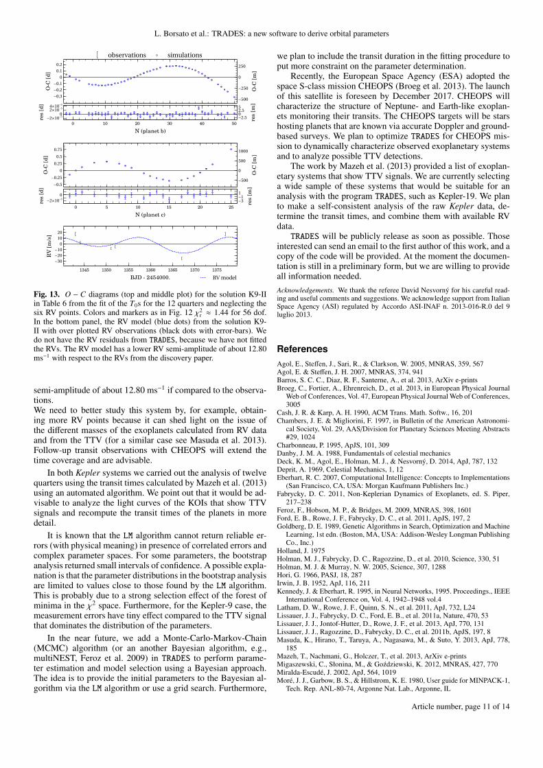
Fig. 13. O − C diagrams (top and middle plot) for the solution K9-IIin Table 6 from the fit of the T0s for the 12 quarters and neglecting thesix RV points. Colors and markers as in Fig. 12 χ2

r ≈ 1.44 for 56 dof.In the bottom panel, the RV model (blue dots) from the solution K9-II with over plotted RV observations (black dots with error-bars). Wedo not have the RV residuals from TRADES, because we have not fittedthe RVs. The RV model has a lower RV semi-amplitude of about 12.80ms−1 with respect to the RVs from the discovery paper.

semi-amplitude of about 12.80 ms−1 if compared to the observa-tions.We need to better study this system by, for example, obtain-ing more RV points because it can shed light on the issue ofthe different masses of the exoplanets calculated from RV dataand from the TTV (for a similar case see Masuda et al. 2013).Follow-up transit observations with CHEOPS will extend thetime coverage and are advisable.

In both Kepler systems we carried out the analysis of twelvequarters using the transit times calculated by Mazeh et al. (2013)using an automated algorithm. We point out that it would be ad-visable to analyze the light curves of the KOIs that show TTVsignals and recompute the transit times of the planets in moredetail.

It is known that the LM algorithm cannot return reliable er-rors (with physical meaning) in presence of correlated errors andcomplex parameter spaces. For some parameters, the bootstrapanalysis returned small intervals of confidence. A possible expla-nation is that the parameter distributions in the bootstrap analysisare limited to values close to those found by the LM algorithm.This is probably due to a strong selection effect of the forest ofminima in the χ2 space. Furthermore, for the Kepler-9 case, themeasurement errors have tiny effect compared to the TTV signalthat dominates the distribution of the parameters.

In the near future, we add a Monte-Carlo-Markov-Chain(MCMC) algorithm (or an another Bayesian algorithm, e.g.,multiNEST, Feroz et al. 2009) in TRADES to perform parame-ter estimation and model selection using a Bayesian approach.The idea is to provide the initial parameters to the Bayesian al-gorithm via the LM algorithm or use a grid search. Furthermore,

we plan to include the transit duration in the fitting procedure toput more constraint on the parameter determination.

Recently, the European Space Agency (ESA) adopted thespace S-class mission CHEOPS (Broeg et al. 2013). The launchof this satellite is foreseen by December 2017. CHEOPS willcharacterize the structure of Neptune- and Earth-like exoplan-ets monitoring their transits. The CHEOPS targets will be starshosting planets that are known via accurate Doppler and ground-based surveys. We plan to optimize TRADES for CHEOPS mis-sion to dynamically characterize observed exoplanetary systemsand to analyze possible TTV detections.

The work by Mazeh et al. (2013) provided a list of exoplan-etary systems that show TTV signals. We are currently selectinga wide sample of these systems that would be suitable for ananalysis with the program TRADES, such as Kepler-19. We planto make a self-consistent analysis of the raw Kepler data, de-termine the transit times, and combine them with available RVdata.TRADES will be publicly release as soon as possible. Those

interested can send an email to the first author of this work, and acopy of the code will be provided. At the moment the documen-tation is still in a preliminary form, but we are willing to provideall information needed.Acknowledgements. We thank the referee David Nesvorný for his careful read-ing and useful comments and suggestions. We acknowledge support from ItalianSpace Agency (ASI) regulated by Accordo ASI-INAF n. 2013-016-R.0 del 9luglio 2013.

ReferencesAgol, E., Steffen, J., Sari, R., & Clarkson, W. 2005, MNRAS, 359, 567Agol, E. & Steffen, J. H. 2007, MNRAS, 374, 941Barros, S. C. C., Diaz, R. F., Santerne, A., et al. 2013, ArXiv e-printsBroeg, C., Fortier, A., Ehrenreich, D., et al. 2013, in European Physical Journal

Web of Conferences, Vol. 47, European Physical Journal Web of Conferences,3005

Cash, J. R. & Karp, A. H. 1990, ACM Trans. Math. Softw., 16, 201Chambers, J. E. & Migliorini, F. 1997, in Bulletin of the American Astronomi-

cal Society, Vol. 29, AAS/Division for Planetary Sciences Meeting Abstracts#29, 1024

Charbonneau, P. 1995, ApJS, 101, 309Danby, J. M. A. 1988, Fundamentals of celestial mechanicsDeck, K. M., Agol, E., Holman, M. J., & Nesvorný, D. 2014, ApJ, 787, 132Deprit, A. 1969, Celestial Mechanics, 1, 12Eberhart, R. C. 2007, Computational Intelligence: Concepts to Implementations

(San Francisco, CA, USA: Morgan Kaufmann Publishers Inc.)Fabrycky, D. C. 2011, Non-Keplerian Dynamics of Exoplanets, ed. S. Piper,

217–238Feroz, F., Hobson, M. P., & Bridges, M. 2009, MNRAS, 398, 1601Ford, E. B., Rowe, J. F., Fabrycky, D. C., et al. 2011, ApJS, 197, 2Goldberg, D. E. 1989, Genetic Algorithms in Search, Optimization and Machine

Learning, 1st edn. (Boston, MA, USA: Addison-Wesley Longman PublishingCo., Inc.)

Holland, J. 1975Holman, M. J., Fabrycky, D. C., Ragozzine, D., et al. 2010, Science, 330, 51Holman, M. J. & Murray, N. W. 2005, Science, 307, 1288Hori, G. 1966, PASJ, 18, 287Irwin, J. B. 1952, ApJ, 116, 211Kennedy, J. & Eberhart, R. 1995, in Neural Networks, 1995. Proceedings., IEEE

International Conference on, Vol. 4, 1942–1948 vol.4Latham, D. W., Rowe, J. F., Quinn, S. N., et al. 2011, ApJ, 732, L24Lissauer, J. J., Fabrycky, D. C., Ford, E. B., et al. 2011a, Nature, 470, 53Lissauer, J. J., Jontof-Hutter, D., Rowe, J. F., et al. 2013, ApJ, 770, 131Lissauer, J. J., Ragozzine, D., Fabrycky, D. C., et al. 2011b, ApJS, 197, 8Masuda, K., Hirano, T., Taruya, A., Nagasawa, M., & Suto, Y. 2013, ApJ, 778,

185Mazeh, T., Nachmani, G., Holczer, T., et al. 2013, ArXiv e-printsMigaszewski, C., Słonina, M., & Gozdziewski, K. 2012, MNRAS, 427, 770Miralda-Escudé, J. 2002, ApJ, 564, 1019Moré, J. J., Garbow, B. S., & Hillstrom, K. E. 1980, User guide for MINPACK-1,

Tech. Rep. ANL-80-74, Argonne Nat. Lab., Argonne, IL



Murray, C. D. & Correia, A. C. M. 2011, Keplerian Orbits and Dynamics ofExoplanets, ed. S. Piper, 15–23

Murray, C. D. & Dermott, S. F. 2000, Solar System DynamicsNascimbeni, V., Piotto, G., Bedin, L. R., & Damasso, M. 2011, A&A, 527, A85Nesvorný, D. 2009, ApJ, 701, 1116Nesvorný, D., Kipping, D., Terrell, D., et al. 2013, ApJ, 777, 3Nesvorný, D. & Morbidelli, A. 2008, ApJ, 688, 636Press, W. H., Teukolsky, S. A., Vetterling, W. T., & Flannery, B. P. 1996, Numer-

ical recipes in Fortran 90 (2nd ed.): the art of parallel scientific computing(New York, NY, USA: Cambridge University Press)

Steffen, J. H. & Agol, E. 2005, MNRAS, 364, L96Tada, T. 2007, Journal of Japan Society of Hydrology & Water Resources, 20,

450Torres, G., Fressin, F., Batalha, N. M., et al. 2011, ApJ, 727, 24Vogt, S. S., Allen, S. L., Bigelow, B. C., et al. 1994, in Society of Photo-Optical

Instrumentation Engineers (SPIE) Conference Series, Vol. 2198, Society ofPhoto-Optical Instrumentation Engineers (SPIE) Conference Series, ed. D. L.Crawford & E. R. Craine, 362



Table 2. Parameters of the Kepler-11 system. Epoch of reference: 2 455 190.0 (BJDUTC).

Parameter Lis2011a K11-Ib K11-IIc Lis2013d K11-IIIe

Mb[M⊕] 5.06 ± 0.95 5.51+1.91−2.04 ± 1.15 5.03+2.29

−2.42 ± 1.50 1.9+1.4−1.0 2.18+1.60

−0.87 ± 0.52

Rb[R⊕] 1.97 ± 0.19 1.80+0.03−0.05

Pb[days] 10.3045 ± 0.0003 10.30459+0.00064−0.00060 ± 0.00035 10.30446+0.00074

−0.00066 ± 0.00070 10.3039+0.006−0.0011 10.30448+0.00033

−0.00032 ± 0.00019

eb 0 0.00018+0.00094−0.00017 ± 0.00494 0.045+0.068

−0.042 0.026+0.026−0.016 ± 0.006

ωb[] 90 89.98+110.02−112.11 ± 220.29 45.00+101.31

−43.34 71.46+2.68−2.63 ± 17.06

Mb[] 73.467 ± 0.003 73.46+0.17−0.15 ± 0.09 73.48111.01

−110.73 ± 219.60 – 91.44+2.28−2.41 ± 16.19

ib[] 88.5+1.0−0.6 89.64+0.36

−0.18

Mc[M⊕] 15.82 ± 2.21 16.11+3.66−4.63 ± 2.30 15.83+4.71

−4.94 ± 3.99 2.9+2.9−1.6 2.09+2.11

−1.43 ± 0.61

Rc[R⊕] 3.15 ± 0.30 2.87+0.05−0.06

Pc[days] 13.0247 ± 0.0003 13.02406+0.00041−0.00046 ± 0.00026 13.02419+0.00045

−0.00054 ± 0.00038 13.0241+0.0013−0.0008 13.02426+0.00053

−0.00058 ± 0.00028

ec 0 0.00005+0.0006−0.00005 ± 0.00375 0.026+0.063

−0.013 0.015+0.011−0.010 ± 0.005

ωc[] 90 90.00+29.61−34.03 ± 100.29 51.34+128.63

−231.00 96.43+0.36−0.24 ± 29.56

Mc[] 288.267 ± 0.005 288.27+0.06−0.06 ± 0.04 288.26+32.04

−31.18 ± 99.66 – 281.99+0.26−0.37 ± 28.71

ic[] 89.0+1.0−0.6 89.59+0.41

−0.16

Md[M⊕] 5.69 ± 1.27 5.97+2.32−2.57 ± 1.36 5.67+2.70

−2.66 ± 1.55 7.3+0.8−1.5 7.24+1.37

−1.36 ± 0.89

Rd[R⊕] 3.43 ± 0.32 3.12+0.06−0.07

Pd[days] 22.6849 ± 0.0007 22.68509+0.00169−0.00167 ± 0.00096 22.68494+0.00173

−0.00202 ± 0.00135 22.6845+0.0010−0.0009 22.68440+0.00095

−0.00095 ± 0.00055

ed 0 0.0001+0.0001−0.0001 ± 0.0074 0.004+0.007

−0.002 0.003+0.007−0.003 ± 0.001

ωd[] 90 90.00+7.72−7.70 ± 77.47 146.31+33.69

−146.31 102.52+0.22−0.51 ± 24.37

Md[] 69.245 ± 0.002 69.25+0.03−0.04 ± 0.02 69.25+7.48

−8.43 ± 76.58 – 56.77+0.23−0.50 ± 24.25

id[] 89.3+0.6−0.4 89.67+0.13

−0.16

Me[M⊕] 8.22 ± 1.58 8.44+3.38−3.49 ± 1.74 8.26+3.25

−3.43 ± 2.03 8.0+1.5−2.1 7.37+1.78

−1.73 ± 0.89

Re[R⊕] 4.52 ± 0.43 4.19+0.07−0.09

Pe[days] 32.0001 ± 0.0008 32.00102+0.00300−0.00366 ± 0.00189 32.00044+0.00342

−0.00377 ± 0.00305 31.9996+0.0008−0.0013 32.00413+0.00173

−0.00207 ± 0.00122

ee 0 0.0002+0.0004−0.0002 ± 0.0089 0.012+0.006

−0.006 0.013+0.003−0.005 ± 0.003

ωe[] 90 90.00+5.82−5.20 ± 1.11 −131.63+29.54

−25.75 204.69+0.26−0.36 ± 3.22

Me[] 122.211 ± 0.003 122.21+0.02−0.02 ± 0.01 122.21+5.01

−6.06 ± 0.04 – 8.86+0.23−0.40 ± 3.19

ie[] 88.8+0.2−0.2 88.89+0.02

−0.02

Mf [M⊕] 1.90 ± 0.95 2.15+1.85−1.76 ± 0.98 2.19+1.98

−1.94 ± 1.23 2.0+0.8−0.9 1.98+1.16

−1.00 ± 0.46

Rf [R⊕] 2.61 ± 0.25 2.49+0.04−0.07

Pf [days] 46.6908 ± 0.0010 46.70131+0.00455−0.00851 ± 0.00304 46.70114+0.00641

−0.00627 ± 0.00688 46.6887+0.0029−0.0038 46.68707+0.00384

−0.00575 ± 0.00143

ef 0 0.000003+0.000001−0.000002 ± 0.000242 0.013+0.011

−0.009 0.005+0.010−0.004 ± 0.002

ωf [] 90 90.00+4.12−4.09 ± 0.03 −24.44+38.48

−47.12 8.58+0.32−0.65 ± 3.41

Mf [] 297.667 ± 0.006 297.68+0.02−0.06 ± 0.02 297.67+4.05

−4.14 ± 0.06 – 18.53+0.27−0.66 ± 3.38

if [] 89.4+0.3−0.2 89.47+0.04

−0.04

Mg[M⊕] < 300 0.00+62.19−0.00 ± 0.21 0.70+0.66

−0.54 ± 41.50 < 25 25.13+48.33−16.83 ± 10.07

Rg[R⊕] 3.66 ± 0.35 3.33+0.06−0.08

Pg[days] 118.3808 ± 0.0025 118.39734+0.00907−0.00959 ± 0.00517 118.39766+0.01080

−0.01053 ± 0.01505 118.3809+0.0012−0.0010 118.38030+0.00361

−0.00309 ± 0.00248

eg 0 0.0029+0.0015−0.0014 ± 0.2974 < 0.15 0.052+0.051

−0.030 ± 0.012

ωg[] 90 90.01+0.63−0.72 ± 0.05 34.51+145.41

−214.50 97.00+0.29−0.17 ± 30.41

Mg[] 211.997 ± 0.005 212.01+0.02−0.02 ± 0.01 212.00+0.71

−0.64 ± 0.05 – 205.71+0.29−0.18 ± 27.38

ig[] 89.8+0.2−0.2 89.87+0.05

−0.06

χ2/dof 110.34/89 110.15/88 110.74/76 341.75/190χ2

r 1.24 1.25 1.46 1.80

Notes. Masses (M), periods (P), eccentricities (e), argument of pericenters (ω), and mean anomaly (M) of the best-fit simulation with 2σ confidenceintervals from bootstrap analysis and ±1σ from LM. Inclinations (i) fixed to the Lis2011 model.(a) Dynamical model as reported in Lissauer et al. (2011a, SI) with circular orbit for each planet, e fixed to 0, and ω fixed to 90(e cosω and e sinω set to zero in the discovery paper).(b) Orbital solution from the analysis of T0s from Lissauer et al. (2011a) for the first three quarters of Kepler data. Parameters fitted:M, P, and M. e fixed to 0 and ω fixed to 90(c) Orbital solution from the analysis of T0s from Lissauer et al. (2011a) for the first three quarters of Kepler data. Parameters fitted:M, P, e, ω, and M.(d) Dynamical model from (Lissauer et al. 2013). Parameters determined from the analysis of 14 quarters of Kepler data. The valuesof the mean anomaly were not reported in the paper (neither the time of passage at the pericenter).(e) Best orbital solution (simulation number 9) of Fig. 6 from the analysis of T0s from Mazeh et al. (2013) for the first 12 quarters ofKepler data. Parameters fitted: M, P, e, ω, and M.



Table 4. Main differences in the Kepler-11 analysis for each solution.

K11-I K11-II K11-IIIQuarters 1 to 3 1 to 3 1 to 12Initial parameters Lis2011 (Lissauer et al. 2011a) K11-I K11-II and e from Lis2013 (Lissauer et al. 2013)Number of fitted parameters 18 30 30Degrees of freedom (dof) 88 76 190TRADES mode LM LM grid (Mg) + LMBootstrap yes yes yesχ2

r 1.25 1.46 1.80

Table 6. Parameters of the Kepler-9 system at epoch tepoch = 2 455 088.212 BJDUTC.

Parameter Holman et al. (2010)a K9-Ib K9-IIc

M?[M] 1.0 ± 0.1R?[R] 1.1 ± 0.09

Mb[MJup] 0.252 ± 0.013 0.246+0.008−0.008 ± 0.014 0.137+0.001

−0.001 ± 0.002Rb[RJup] 0.842 ± 0.069Pb[days] 19.2372 ± 0.0007 19.23686+0.00041

−0.00032 ± 0.00051 19.23876+0.00004−0.00004 ± 0.00006

eb 0.151 ± 0.034 0.131+0.008−0.006 ± 0.016 0.058+0.001

−0.001 ± 0.002ib[] 88.55 ± 0.25ωb[] 18.56 ± 13.69 18.91+0.60

−0.92 ± 14.58 356.06+0.11−0.21 ± 0.44

Mb[] 332.15 ± 14.06 333.79+0.89−0.97 ± 14.27 3.78+0.22

−0.20 ± 0.60Ωb[] 0 (fixed)

Mc[MJup] 0.171 ± 0.013 0.169+0.005−0.006 ± 0.017 0.094+0.001

−0.001 ± 0.002Rc[RJup] 0.823 ± 0.067Pc[days] 38.992 ± 0.005 38.97897+0.00182

−0.00222 ± 0.00336 38.98610+0.00020−0.00021 ± 0.00043

ec 0.133 ± 0.039 0.119+0.004−0.003 ± 0.012 0.068+0.001

−0.001 ± 0.001ic[] 89.12 ± 0.17d

ωc[] 101.31 ± 47.05 102.85+0.43−0.51 ± 8.04 167.57+0.01

−0.01 ± 0.01Mc[] 6.89 ± 47.20 7.48+0.41

−0.35 ± 6.10 307.43+0.06−0.05 ± 0.07

Ωc[] 2 ± 3 1.63+0.07−0.11 ± 1.19 359.89+0.30

−0.98 ± 0.02

χ2/dof 28.382/10 80.852/56χ2

r 2.84 1.44

Notes. Results for the analysis of the Kepler-9 system with TRADES using the masses, the period, the eccentricity, the argument of pericenter, themean anomaly of both planets, and the longitude of node of Kepler-9c as fitting parameters.(a) Parameters from the SOM of Holman et al. (2010).(b) Analysis of TRADES with initial parameters and T0s from Holman et al. (2010, SOM). Transits and RVs fit.(c) Analysis with TRADES+PSO+LM and T0s from Mazeh et al. (2013). Initial parameter boundaries were large enough to contains both solutionsK9-I and by Holman et al. (2010). We fit only the transit times, and ignored the six RV points.(d) The authors confirmed a typo in the inclination of Kepler-9c in the SOM (Holman 2012, priv. comm.), considering that the value of 88.12reported is inconsistent with the transit geometry.


trades: a new software to derive orbital parameters from

Documents