traffic fatalities and economic growth - … · 1 traffic fatalities and economic growth elizabeth...

TRAFFIC FATALITIES AND ECONOMIC GROWTH

Elizabeth Kopits University of Maryland and Resources for the Future

Maureen Cropper

World Bank

World Bank Policy Research Working Paper 3035, April 2003 The Policy Research Working Paper Series disseminates the findings of work in progress to encourage the exchange of ideas about development issues. An objective of the series is to get the findings out quickly, even if the presentations are less than fully polished. The papers carry the names of the authors and should be cited accordingly. The findings, interpretations, and conclusions expressed in this paper are entirely those of the authors. They do not necessarily represent the view of the World Bank, its Executive Directors, or the countries they represent. Policy Research Working Papers are available online at http://econ.worldbank.org.

We would like to thank the World Bank Research Board for funding and the Bank’s Road Safety Thematic Group for comments and encouragement. We would especially like to thank Zmarak Shalizi for his encouragement during early stages of the project. Paulus Guitink and Hua Wang generously provided data. We would also like to thank the following people for their comments and suggestions: Amy Aeron-Thomas, Roger Betancourt, Bill Evans, Goff Jacobs, Matthijs Koornstra, Seth Sanders, Jeff Smith, V. Kerry Smith, and Jagadish Guria for his careful reading of the paper. We appreciate the comments of seminar participants at Resources for the Future, the University of Maryland, Camp Resources and the International Conference on Vehicle Safety and Reliability in Keszthely, Hungary.

1

Traffic Fatalities and Economic Growth Elizabeth Kopits and Maureen Cropper

I. Introduction

As countries develop death rates usually fall, especially for diseases that affect the

young and result in substantial life-years lost. Deaths due to traffic accidents are a

notable exception: the growth in motor vehicles that accompanies economic growth

usually brings an increase in road traffic accidents. Indeed, the World Health

Organization has predicted that traffic fatalities will be the sixth leading cause of death

worldwide and the second leading cause of disability-adjusted life-years lost in

developing countries by the year 2020 (Murray and Lopez 1996). Table 1 highlights the

increasing importance of the problem in several developing countries. For example,

between 1975 and 1998, road traffic deaths per capita increased by 44% in Malaysia and

by over 200% in Colombia and Botswana.

The situation in high- income countries is quite different. Over the same period,

traffic fatalities per person decreased by 60% in Canada and Hong Kong, and by amounts

ranging from 25% to 50% in most European countries. This reflects a downward trend in

both the fatality rate (deaths/population) and in fatalities per kilometer traveled that began

in most OECD countries in the early 1970’s and has continued to the present.

2

Table 1. Change in Traffic Fatality Rate (Deaths/10,000 Persons), 1975-1998

Country % Change (‘75-’98) Country

% Change (‘75-’98)

Canada -63.4% Malaysia 44.3% Hong Kong -61.7% India^ 79.3% Finland -59.8% Sri Lanka 84.5% Austria -59.1% Lesotho 192.8% Sweden -58.3% Colombia 237.1% Israel -49.7% China 243.0% Belgium -43.8% Botswana** 383.8% France -42.6% Italy* -36.7% New Zealand -33.2% Taiwan -32.0% United States -27.2% Japan -24.5% *%change (‘75-‘97), **%change (‘76-‘98), ^%change (’80-’98).

These patterns are not surprising. The traffic fatality rate (fatalities/population) is

the product of vehicles per person (V/P) and fatalities per vehicle (F/V). How rapidly

fatality risk grows depends, by definition, on the rate of growth in motorization (V/P) and

the rate of change in fatalities per vehicle (F/V).1 In most developing countries over the

past 25 years, vehicle ownership grew more rapidly than fatalities per vehicle fell. The

experience in industrialized countries, however, was the opposite; vehicles per person

grew more slowly than fatalities per vehicle fell. From these observations, two questions

emerge: Why did these patterns occur? and What trends can be expected in the future?

To answer these questions we examine how the death rate (F/P) associated with

traffic accidents and its components—V/P and F/V—change as countries grow. The

topic is of interest for two reasons. For planning purposes it important to forecast the

growth in traffic fatalities. Equations relating F/P to per capita income can be used to

1The fatality rate may also be expressed as the product of fatalities per vehicle kilometers traveled (F/VKT) and distance traveled per person (VKT/P). Lack of reliable time -series VKT data, especially. for developing countries, prevents us from using this measure for our analysis.

3

predict traffic fatalities by region. These forecasts should alert policymakers to what is

likely to happen if measures are not enacted to reduce traffic accidents.

A second motive for our work comes from the literature on Environmental

Kuznets Curves (Grossman and Krueger 1995). This literature examines the relationship

between environmental externalities, such as air and water pollution, and economic

growth. A focus of this literature has been in identifying the income levels at which

externalities begin to decline. Road traffic fatalities are, indeed, an externality associated

with motorization, especially in developing countries where pedestrians comprise a large

share of casualties and motorists are often not insured. It is of interest to examine the

income level at which the traffic fatality rate (F/P) historically has begun to decline and

to compare this with the pattern observed for other externalities.

We investigate these issues by estimating equations for the motor vehicle fatality

rate (F/P), the rate of motorization (V/P) and fatalities per vehicle (F/V) using panel data

from 1963-99 for 88 countries. We estimate fixed effects models in which the natural

logarithm of F/P, V/P and F/V are expressed as (a) a quadratic function of ln(Y) and (b) a

spline function of ln(Y), where Y = real per capita GDP (measured in 1985 international

prices). Time trends during the period 1963-99 are modeled in four ways: (1) a common

linear time trend; (2) a common log- linear time trend; (3) regional, linear time trends; and

(4) regional, log-linear time trends. These models are used to project traffic fatalities and

the stock of motor vehicles to 2020.

Our main results are as follows. The per capita income at which the motor

vehicle fatality rate begins to decline is in the range of incomes at which other

externalities (specifically the common air pollutants) begin to decline—approximately

4

$6100 (1985 international dollars) when a common time trend is assumed for all

countries and $8600 (1985 international dollars) when separate time trends are used for

each geographic region. This turning point is driven by the rate of decline in F/V as

income rises since V/P, while increasing with income at a decreasing rate, never declines

with economic growth.

Projections of future traffic fatalities suggest that the global road death toll will

grow by approximately 66% over the next twenty years. This number, however, reflects

divergent rates of change in different parts of the world: a decline in fatalities in high-

income countries of approximately 28% versus an increase in fatalities of almost 92% in

China and 147% in India. We also predict that the fatality rate will rise to

approximately 2 per 10,000 persons in developing countries by 2020, while it will fall to

less than 1 per 10,000 in high- income countries.

The paper is organized at follows. Section II presents trends in fatality rates

(F/P), motorization rates (V/P), and fatalities per vehicle (F/V) for various countries.

Plots of each variable against per capita income motivate our econometric models.

Section III describes the econometric models estimated and Section IV presents our

projections of road traffic fatalities. Section V concludes.

II. How Fatality Risk, Motorization Rates and Fatalities/Vehicle Vary Across (and Within) Countries

Death rates (F/P) due to motor vehicle crashes are the product of the motorization

rate (V/P) and fatalities per motor vehicle (F/V). Before estimating statistical models

relating these ratios to per capita income it is useful to examine data showing how these

quantities vary with income both within and across countries.

5

It is widely recognized that the motorization rate rises with income (Ingram and

Liu (1999), Dargay and Gately (1999), Button et al. (1993)), implying that one should

find large differences in vehicles per capita across countries at different stages of

development and within countries as per capita incomes grow. Table 2 presents data on

motorization rates for various countries in 1999.2 Figure 1 plots the motorization rates

for these countries against per capita income, pooling data from all countries and years,

while Figure 2 shows how motorization rates have grown with income over time for a

sample of countries.

Table 2. Motorization Rates, 1999, 60 Countries

Country Vehicles*

/1,000 Persons Country Vehicles*

/1,000 Persons

HD1 Countries: HD2 Countries: United States 779 Malaysia 451 Luxembourg 685 Bulgaria 342 Japan1 677 Thailand3 280 Italy2 658 Latvia 267 Iceland 629 Mauritius 195 Switzerland 622 Romania 169 Australia3 616 South Africa 144 Austria 612 Panama2 112 Canada1 585 Turkey 100 Germany1 572 Indonesia1 81 New Zealand2 565 Sri Lanka1 74 Norway 559 Botswana 72 Cyprus 551 Swaziland1 69 Belgium 522 Colombia 67 Spain2 499 Benin3 52 Finland 498 Morocco 51 Sweden1 496 Ecuador1 47 Czechoslovakia 440 Philippines1 42 2The data in Table 2 and Figure 1 are displayed according to development status. Observations for countries with a UN Human Development Index (HDI) less than 0.8 are denoted as “HD2” and countries with an HDI value greater than 0.8 are labeled as “HD1”.

6

United Kingdom1 434 Togo3 39 Netherlands 427 Mongolia 38 Denmark 424 Egypt3 35 Portugal2 423 India2 34 Bahrain 339 Nigeria3 29 Poland 323 Pakistan 23 Ireland3 312 Kenya3 14 Israel 301 Senegal3 14 Korea, Rep. 296 Bangladesh2 3.1 Hungary 283 Ethiopia1 1.5 Singapore 164 Costa Rica 162 Chile 138 Hong Kong 80

*Including passenger cars, buses, trucks, and motorized two-wheelers. 1- 1998 data, 2- 1997 data, 3- 1996 data.

Figure 1. Motorization Rate vs. Income: All Countries and Years

Veh

icle

s/10

,000

Pers

ons

Per Capita GDP, 1985 int'l$0 5,000 10,000 15,000 20,000 25,000

0

2,000

4,000

6,000

8,000

HD1 Observations HD2 Observations

The cross-sectional variation in motorization rates in Table 2 is striking. Vehicles

per capita range from a high of 780 per 1,000 persons in the United States to fewer than

30 per 1,000 persons in countries such as Pakistan and Nigeria. High- income countries

7

tend to have more vehicles per capita than lower income countries but there are important

exceptions. Low motorization rates in Hong Kong, Singapore, Chile, and Costa Rica are

notable outliers. Figure 1, which plots data on V/P for all countries and years in the

dataset, suggests that, overall, motorization is strongly correlated with income. The

within-group variation in motorization varies from country to country, however, as

shown in Figure 2. Growth in vehicle ownership appears to have slowed down (but not

declined) in many high- income countries such as Norway, Australia, Hong Kong, and the

United States. In countries experiencing lower levels of per capita GDP such as Greece,

Malaysia, and Thailand, however, vehicle fleets have continued to expand rapidly with

income in recent decades.

8

Figure 2. Motorization Rates vs. Income: Selected Countries

Veh

icle

s/10

,000

Pers

ons

Per Capita GDP, 1985 int'l$3,000 6,000 9,000 12,000 15,000 18,000 21,000

0

1000

2000

3000

4000

5000

6000

7000

8000

Greece Korea, Rep. of United States Hong Kong Norway Australia Taiwan, Province of China

Veh

icle

s/10

,000

Pers

ons


0

500

1000

1500

2000

2500

3000

3500

4000

4500

Mauritius Thailand Turkey Botswana Malaysia Sri Lanka

9

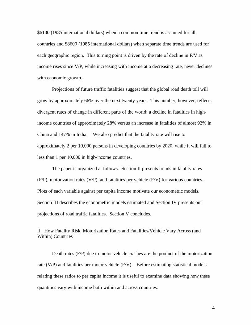
Fatalities per vehicle, by contrast, appear to decline steadily with income, at least

after some low level of income, and then reach a floor. Both Figure 3, which plots the

fatality rate (F/V) against income using data for all countries and years, and Figure 4,

which shows how F/V has changed with income over time for a sample of countries,

attest to this fact.3 In part, the sharp decline in F/V with income reflects the fact that, as

income rises, a higher percentage of travelers are vehicle passengers rather than

pedestrians, and thus, are less likely to die in the event of a crash. 4 It also may reflect the

move to safer vehicles (e.g., from two-wheelers to four-wheelers), safer roads, and/or

changing attitudes toward risk as incomes grow.

Figure 3. Fatalities/Vehicle vs. Income: All Countries and Years

Fata

litie

s/10

,000

Veh

icle

s


0

50

100

150

200

250


3The fatality figures used in Figures 3 and 4 have not been adjusted for underreporting of road deaths. Thus, F/V levels in developing countries may be underestimated. 4 This point was first publicized by Smeed (1949), who demonstrated that F/V declines as V/P increases.

10

Figure 4. Fatalities/Vehicle v. Income: Selected Countries

Fata

litie

s/10

,000

Veh

icle

s


0

50

100

150

200

250

Bangladesh Egypt Uganda Ethiopia Morocco India Turkey Mauritius Malaysia Korea, Rep. of

Fata

litie

s/10

,000

Veh

icle

s

Per Capita GDP, 1985 int'l$2,000 8,000 14,000 20,000

0

10

20

30

40

Greece United States Hong Kong Norway Australia Taiwan, Province of China

11

The foregoing data suggest that one would expect to see the motor vehicle fatality

rate (F/P) first increase and then decrease with income. Figure 5, which plots of F/P

versus income for all years and countries in our dataset, supports this inverted U-shaped

pattern. As incomes grow and vehicle fleets increase during initial stages of

development, traffic fatality rates tend to worsen. At higher income levels, however, as

growth in motorization slows and governments and individuals invest more in road

safety, the decline in F/V drives the fatality rate (F/P) down.

Figure 5. Traffic Fatality Rate vs. Income: All Countries and Years

Fata

litie

s/10

,000

Pers

ons


0

1

2

3

4


12

III. Statistical Models of Fatalities, Vehicle Ownership and Economic Growth

A. Models of Fatalities per Person

In fitting statistical models to the data on fatality risk we employ models of the

general form:

(1) ln(F/P)it = ai + G(t) + F[ln(Yit)] + eit

where F/P = Fatalities/10,000 Persons, Y = Real Per Capita GDP (measured in 1985

international prices), ai is a country-specific intercept, and G and F are functions. Two

specific forms of F are used, a quadratic specification (equation (2)) and a spline

(piecewise linear) specification (equation (3)):

(2) ln(F/P)it = ai + G(t) + b lnYit + c (lnYit)2 + eit

(3) ln(F/P)it = ai + G(t) + b lnYit + Ss [csDs(lnYit – lnYs)] + eit

where Ds is a dummy variable = 1 if Yit is in income category s+1, and Ys is the cutoff

income value between the s and s+1 income group. Following Schmalensee et al. (2000),

we divide the observations into 10 income groups with an equal number of observations

in each spline segment.

Four different forms of G(t) are used: (1) a common linear time trend; (2) a

common log- linear time trend (ln t); (3) regional, linear time trends; and (4) regional, log-

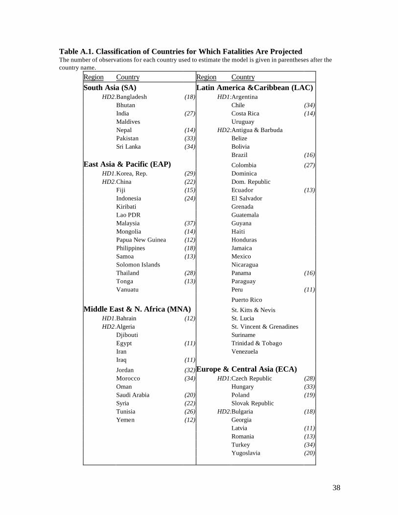
linear (ln t) time trends. For purposes of defining time trends, we divide countries into

two groups: highly developed countries (HD1)—i.e., countries that have a Human

Development Index in 1999 of 0.8 or greater—and all other countries (HD2).5 In

practice, this division of countries (shown in detail in the Appendix) corresponds closely

5 The United Nations Human Development Index measures per capita income, life expectancy and educational achievement.

13

to highly-motorized countries versus other countries. All HD1 countries are treated as a

single region for the purposes of computing time trends. HD2 countries, in turn, are

classified according to region. Table 3 shows the number of countries in each geographic

region, for both HD1 and HD2 countries.

Table 3. Regional Distribution of Countries Used in Model Estimation

WB Region HD2 HD1

East Asia & Pacific 10 1 E. Europe & Central Asia 5 3 Latin America & Caribbean 5 2 Middle East & North Africa 8 1 South Asia 5 Sub-Saharan Africa 20 High-Income Countries 28

Total: 53 35

The inclusion of country-specific intercepts in equation (1) implies that the impact

of income on the fatality rate will reflect within- rather than between-country variation in

ln(F/P) and ln(Y). This is desirable for two reasons. For the purposes of predicting

future trends in F/P it is more desirable to rely on within-country experience rather than

on largely cross-sectional variation in income and fatality risk. Using only cross-country

variation to predict the future pattern of traffic fatalities is equivalent to saying that once

Indonesia reaches the income level of Greece, its road safety record will mirror that of

Greece. The second reason is that countries differ in their definition of what constitutes a

traffic death and in the percentage of deaths that are reported. (This topic is discussed

more fully in Section IV.) To the extent that the degree of under-reporting remains

14

constant over time but varies across countries it will not affect estimates of the impact of

economic growth on fatality risk.6

Equations (2) and (3) are estimated using pane l data for 88 countries for the

period 1963-99. To be included in the dataset a country must have at least 10 years of

data on traffic fatalities. Table A.1 in the Appendix lists the countries used to estimate

the models and the number of years of data that are available for each country. The data

on traffic fatalities used in this study come primarily from the International Road

Federation Yearbooks, which have been supplemented by and cross-checked against

various other sources. The sources of traffic fatality and all other data are described in

the Appendix.

B. Empirical Results

Table 4 summarizes the results of estimating the 8 models formed by combining

the quadratic and spline functions with 4 methods of treating time trends. (Complete

regression results are displayed in Table A.2. in the Appendix.) The table shows the

income level at which F/P first begins to decline as well as the time coefficients for each

model. To give a more complete picture of the model results, Figures 6 and 7 plot F/P as

a function of per capita income.7 Figure 6 shows the quadratic and spline models with a

common linear time trend while Figure 7 plots the quadratic and spline models with

region-specific log- linear time trends.

6 To illustrate, when equation (2) is estimated using country-specific intercepts, the coefficients b and c reflect within-country variation in fatalities and income. Multiplying country i’s fatality rate by a constant to reflect under-reporting would not change the estimates of b and c. 7In both figures, F/P results are displayed using the country intercept for India with the time trend set equal to 1999.

15

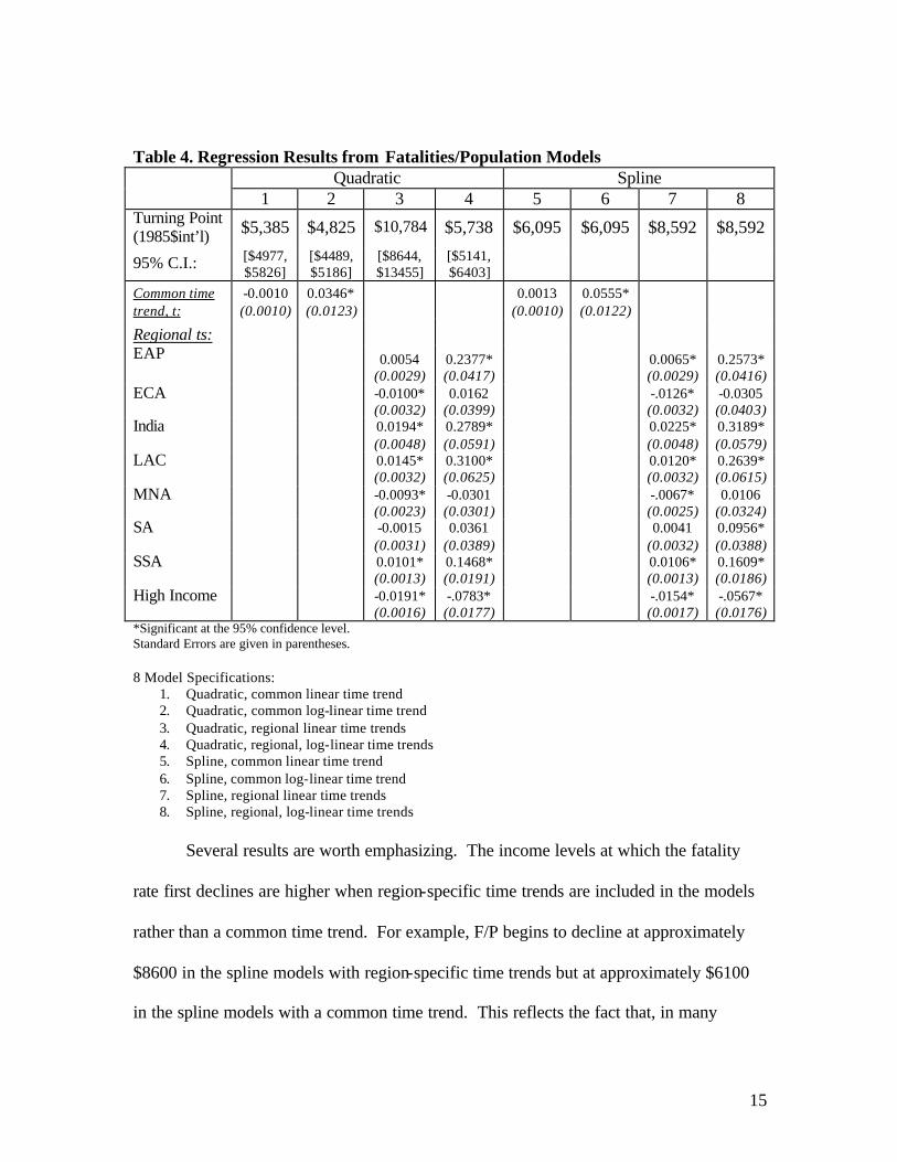
Table 4. Regression Results from Fatalities/Population Models Quadratic Spline 1 2 3 4 5 6 7 8 Turning Point (1985$int’l) $5,385 $4,825 $10,784 $5,738 $6,095 $6,095 $8,592 $8,592

95% C.I.: [$4977, $5826]

[$4489, $5186]

[$8644, $13455]

[$5141, $6403]

Common time trend, t:

-0.0010 (0.0010)

0.0346* (0.0123)

0.0013 (0.0010)

0.0555* (0.0122)

Regional ts: EAP

0.0054

(0.0029) 0.2377* (0.0417)

0.0065* (0.0029)

0.2573* (0.0416)

ECA

-0.0100* (0.0032)

0.0162 (0.0399)

-.0126* (0.0032)

-0.0305 (0.0403)

India

0.0194* (0.0048)

0.2789* (0.0591)

0.0225* (0.0048)

0.3189* (0.0579)

LAC

0.0145* (0.0032)

0.3100* (0.0625)

0.0120* (0.0032)

0.2639* (0.0615)

MNA

-0.0093* (0.0023)

-0.0301 (0.0301)

-.0067* (0.0025)

0.0106 (0.0324)

SA

-0.0015 (0.0031)

0.0361 (0.0389)

0.0041 (0.0032)

0.0956* (0.0388)

SSA

0.0101* (0.0013)

0.1468* (0.0191)

0.0106* (0.0013)

0.1609* (0.0186)

High Income

-0.0191* (0.0016)

-.0783* (0.0177)

-.0154* (0.0017)

-.0567* (0.0176)

*Significant at the 95% confidence level. Standard Errors are given in parentheses.

8 Model Specifications: 1. Quadratic, common linear time trend 2. Quadratic, common log-linear time trend 3. Quadratic, regional linear time trends 4. Quadratic, regional, log-linear time trends 5. Spline, common linear time trend 6. Spline, common log-linear time trend 7. Spline, regional linear time trends 8. Spline, regional, log-linear time trends

Several results are worth emphasizing. The income levels at which the fatality

rate first declines are higher when region-specific time trends are included in the models

rather than a common time trend. For example, F/P begins to decline at approximately

$8600 in the spline models with region-specific time trends but at approximately $6100

in the spline models with a common time trend. This reflects the fact that, in many

16

developing countries, fatality risk over the period 1963-99 grew faster than could be

explained by income growth alone. Because the region-specific time trends are jointly

significant, we believe that more emphasis should be placed on these models than on

models with a common time trend.

Whether the time trend enters the models linearly or in log- linear form, the

differences in trends across regions are generally similar. Over the estimation period

(1963-99) the fatality rate grew fastest in India and in Latin America (LAC) (holding

income constant), and almost as fast in Sub-Saharan Africa as in LAC. By contrast,

(holding income constant) F/P declined in high- income countries. Results for other

regions are statistically insignificant in at least some specifications.

Figure 6. Fatalities/Population Results, Common Linear Time Trend

0

0.2

0.4

0.6

0.8

1

1.2

1.4

1.6

1.8

200 4,200 8,200 12,200 16,200 20,200 24,200 28,200

Per Capita GDP (1985 $int'l)

Fata

litie

s/10

,000

Pers

ons

Quadratic,commonT

Spline,commonT

17

Figure 7. Fatalities/Population Results, Log-Linear Regional Time Trends

It is also clear from examining Figures 6 and 7 that the relationship between per

capita income and the fatality rate is quite similar (holding the treatment of time constant)

whether one uses the quadratic or spline function. When a common time trend is

assumed F/P begins to decline at an income of $5,400 using the quadratic specification

and at an income of $6,100 with the spline model. When region-specific, log- linear time

trends are included F/P begins to decline at an income of $5,700 in the quadratic model

and at an income of $8,600 in the spline model. In both figures, the two models are

almost identical at low levels of income; however, the fatality rate peaks at a higher level

of income in the spline model and falls faster than in the quadratic model after it peaks.

In the Kuznets Curve literature it is standard practice to focus on the income level

at which the externality in question begins to decline. The usual interpretation is that, if a

0

0.2

0.4

0.6

0.8

1

1.2

1.4

1.6

1.8

200 4,200 8,200 12,200 16,200 20,200 24,200 28,200


Fata

litie

s/10

,000

Pers

ons

Quadratic,ln(regionalT)

Spline,ln(regionalT)

18

country follows historical trends, the problem in question will eventually lessen once per

capita income reaches this turning point. Because the spline is a more flexible functional

form, we focus on the spline results in Table 4. The income levels at which fatalities per

person peak in the spline models, $6100 and $8600 (1985 international dollars) are within

the range of incomes at which Kuznets curves for common air and water pollutants peak

(Grossman and Krueger 1995). To better understand why this occurs, in the next sections

we examine models similar to those in Table 4 for the two components of fatalities per

person—vehicles per person and fatalities per vehicle.

C. Models of Vehicles per Person

Models for vehicles per person (V/P) are summarized in Table 5 and Figure 8.

Table 5 shows how motorization (V/P) varies with income in the both the quadratic and

spline models. Our discussion, however, focuses on the spline models. Figure 8 plots the

four spline models using the country intercept for India, with the time trend set equal to

1999.

Of the four spline models in Table 5, only two (Models 6 and 8) show vehicles

per person increasing with per capita income at a decreasing rate for all relevant values of

per capita income. This result occurs when time is entered in a log-linear fashion; when it

enters the motorization equation linearly, V/P peaks at a value of income observed in the

data, and the time trend associated with vehicle ownership is large and positive. The log-

linear time trend thus seems to yield more reasonable results than the linear. Of the two

models with log- linear time trends, only the model with regional log- linear time trends

19

yields non-negative income elasticities for all levels of income; hence we focus on this

model.

Figure 8. Vehicles/Population Results, Spline Models Notes for Table 5:

Standard Errors are given in parentheses. The constant term reflects the intercept term for India. Country fixed effects were included in all regressions but are not displayed here. Asterisks indicate significance at the 95% confidence level.

Model Specifications:

1. Quadratic, common linear time trend 2. Quadratic, common log-linear time trend 3. Quadratic, regional linear time trends 4. Quadratic, regional, log-linear time trends 5. Spline, common linear time trend 6. Spline, common log-linear time trend 7. Spline, regional linear time trends 8. Spline, regional, log-linear time trends

0

50

100

150

200

250

300

$200 $4,200 $8,200 $12,200 $16,200 $20,200 $24,200 $28,200


Veh

icle

s pe

r 1,0

00 P

erso

ns

ln(regionalT)ln(commonT)commonTregionalT

20

Table 5. Regression Results from Vehicles/Population Models Quadratic Spline Independent

Variables 1 2 3 4 5 6 7 8

LnY 5.5228* (0.2120)

5.0464* (0.2301)

3.0785* (0.2976)

3.0826* (0.3042)

(lnYit)2 -0.2860* (0.0129)

-0.2407* (0.0138)

-0.1420* (0.0182)

-0.1242* (0.0183)

lnY for: $1 - $946

0.8569* (0.1281)

0.9551* (0.1473)

0.4247* (0.1239)

0.1899 (0.1471)

$946 - $1,535 1.4314* (0.1020)

1.7748* (0.1149)

0.9087* (0.1088)

1.6752* (0.1168)

$1,535 - $2,290 0.6748* (0.1027)

1.0435* (0.1157)

0.7078* (0.1139)

1.0849* (0.1258)

$2,290 - $3,441 1.3786* (0.1115)

1.5083* (0.1285)

0.8825* (0.1127)

1.0385* (0.1332)

$3,441 - $4,682 1.2179* (0.1347)

1.5702* (0.1524)

1.1359* (0.1250)

1.5656* (0.1426)

$4,682 - $6,911 0.8052* (0.1025)

1.1438* (0.1156)

0.8378* (0.0955)

1.1870* (0.1081)

$6,911 - $9,238 0.5691* (0.1267)

0.5949* (0.1462)

0.6883* (0.1193)

0.8223* (0.1399)

$9,238-$11,263 -0.4359* (0.1756)

-0.0216 (0.1999)

-0.3367* (0.1663)

0.1884 (0.1902)

$11,263-13,663 -0.7142* (0.1750)

0.2125 (0.1941)

-0.5504* (0.1693)

0.4123* (0.1835)

> $13,663 -0.6119* (0.1477)

0.0978 (0.1650)

-0.5092* (0.1396)

0.1897 (0.1540)

Turning Point (1985$int’l)

$15,587 $35,723 $51,179 $244117 $9,238 - $9,238 -

95% C.I.: [$12995, $18,696]

[$26690,$47,813]

[$24,687, $106099]

[$71,420,$834411]

Common time trend: t

0.0281* (0.0010)

0.2358* (0.0132)

0.0322* (0.0010)

0.2631* (0.0130)

Regional t: EAP

0.0539* (0.0027)

0.5587* (0.0417)

0.0582* (0.0026)

0.5990* (0.0418)

ECA 0.0597* (0.0031)

0.5400* (0.0389)

0.0559* (0.0030)

0.5046* (0.0400)

India 0.0657* (0.0039)

0.6619* (0.0501)

0.0747* (0.0037)

0.7331* (0.0483)

LAC 0.0256* (0.0042)

0.2184* (0.0574)

0.0234* (0.0040)

0.2017* (0.0572)

MNA 0.0157* (0.0029)

0.0449* (0.0368)

0.0201* (0.0030)

0.0358 (0.0385)

SA

0.0359* (0.0027)

0.2547* (0.0365)

0.0406* (0.0027)

0.2468* (0.0361)

SSA 0.0290* (0.0014)

0.3119* (0.0202)

0.0304* (0.0013)

0.3529* (0.0196)

High Income 0.0215* (0.0014)

0.1604* (0.0168)

0.0292* (0.0014)

0.1977* (0.0168)

F statistic on regional ts: F8,1791 =

151.15 F8,1791 =

80.03 F8,1783 =

202.95 F8,1783 =

96.64

Constant -20.688* (0.8645)

-19.675* (0.9430)

-11.378* (1.1795)

-12.806* (1.2143)

-2.2872* (0.8586)

-3.1038* (0.9835)

-0.0692 (0.8261)

0.8421 (0.9753)

Adjusted R2: 0.9783 0.9742 0.9818 0.9775 0.9820 0.9767 0.9849 0.9799 No. of Countries: 75, No. of observations: 1876

21

In the preferred model, Model 8, the income elasticity of vehicle ownership

attains a maximum value of 1.67 in the second spline segment ($946 - $1,535 (1985

international dollars)) and decreases to a low of 0.18 in the highest income category.

Above the lowest income category, income elasticities in income categories 2 through 5

are significantly higher than income elasticities in income categories 7 to 10.8 These

results are broadly consistent with previous studies of motorization, which find that the

income elasticity of demand for motor vehicles declines with income (Ingram and Liu

(1998), Dargay and Gately (1999), Button et al. (1993)). Figure 8 suggests that the rate

of increase in motorization slows down considerably after reaching a per capita income

of $9400 (1985 international dollars), the level of income attained by Norway and the

United Kingdom in 1974.

D. Models for Fatalities per Vehicle

Table 6 and Figure 9 confirm that fatalities per vehicle decline sharply with

income. Focusing once again on the spline models with log-linear time trends, F/V

declines with income for per capita GDP in excess of $1,180 (1985 international dollars)

when either common or regional log- linear time trends are used. Figure 9, which plots

the four spline models for India (t = 1999) indicates exactly how fast F/V declines as

income grows. Fatalities per vehicle decline by a factor of 3 (e.g., from 360 to 120 per

100,000 vehicles for India) as per capita income grows from $1200 to $4400. After

reaching a per capita income of $15,200 (1985 international dollars), however, F/V

8 Income elasticity estimates generated from a two-segment spline model are statistically different from each other, decreasing from 1.32 (0.051) to 0.719 (0.052) once per capita income exceeds $4,682 (1985 international dollars).

22

Table 6. Regression Results from Fatalities/Vehicles Models

Quadratic Spline Independent Variables 1 2 3 4 5 6 7 8

LnY 2.3796* (0.2509)

3.0043* (0.2915)

2.2926* (0.3829)

3.0550* (0.4240)

(lnYit)2 -0.1612* (0.0151)

-0.2313* (0.0173)

-0.1458* (0.0231)

-0.2340* (0.0252)

lnY for: $1-$1,179

0.6190* (0.1167)

0.3024* (0.1372)

1.0517* (0.1268)

0.6548* (0.1551)

$1,179-$1,730 -0.2292 (0.1468)

-0.9258* (0.1697)

-0.5022* (0.1585)

-1.5227* (0.1867)

$1,730-$2,698 0.2538

(0.1334) -0.2607 (0.1552)

0.4462* (0.1426)

-0.2433 (0.1711)

$2,698-$3,813 -0.5814* (0.1485)

-1.0952* (0.1751)

-0.0908 (0.1519)

-0.8321* (0.1834)

$3,813-$5,391 -0.3880* (0.1415)

-0.9340* (0.1640)

-0.1747 (0.1359)

-0.8727* (0.1620)

$5,391-$7,532 -0.5550* (0.1447)

-1.0029* (0.1686)

-0.4913* (0.1391)

-1.0357* (0.1668)

$7,532-$9,614 -0.6347* (0.1745)

-0.9444* (0.2075)

-0.3684* (0.1697)

-0.8750* (0.2083)

$9,614-$11,469 -0.2826 (0.2421)

-1.1976* (0.2824)

0.0859 (0.2354)

-1.1407* (0.2810)

$11,469-13,682 -0.4438 (0.2363)

-1.8455* (0.2690)

0.0051 (0.2333)

-1.7977* (0.2664)

>$13,682 -0.2782 (0.1905)

-1.2485* (0.2185)

0.0143 (0.1855)

-1.2226* (0.2151)


$1,603 $661 $2,593 $683 $2,698 $1,179 $2,698 $1,179

95% C.I.: [$1,189, $2,161]

[$475, $920]

[$1,859, $3,616]

[$440, $1,061]


-0.0370* (0.0013)

-0.2335* (0.0170)

-0.0386* (0.0013)

-0.2285* (0.0176)

Regional t: EAP

-0.0512* (0.0034)

-0.2661* (0.0540)

-0.0561* (0.0034)

-0.2826* (0.0560)

ECA -0.0671* (0.0036)

-0.4416* (0.0487)

-0.0698* (0.0038)

-0.4609* (0.0522)

India -0.0445* (0.0049)

-0.3551* (0.0686)

-0.0536* (0.0050)

-0.4416* (0.0701)

LAC -0.0123* (0.0060)

-0.0219 (0.1362)

-0.0127* (0.0061)

-0.0142 (0.1387)

MNA -0.0268* (0.0035)

-0.0503 (0.0490) -0.0234*

(0.0039) 0.0922

(0.0543)

SA

-0.0392* (0.0033)

-0.1925* (0.0462) -0.0375*

(0.0035) -0.1230* (0.0473)

SSA -0.0289* (0.0020)

-0.2527* (0.0311)

-0.0284* (0.0019)

-0.2365* (0.0306)

High Income -0.0424* (0.0017)

-0.2293* (0.0215) -0.0470*

(0.0018) -0.2450* (0.0223)


132.45 F8,1615 =

29.78 F8,1607 =

140.67 F8,1607 =

31.56

Constant -11.105* (1.0305)

-12.166* (1.2035)

-11.092* (1.5275)

-12.055* (1.7003)

-6.5829* (0.7967)

-4.5175* (0.9333)

-9.2431* (0.8365)

-6.3274* (1.0105)


23

declines very slowly in absolute terms: from 25 per 100,000 vehicles at an income of

$20,000 to 15 per 100,000 vehicles at an income of $30,000.

Figure 9. Fatalities/Vehicle Results, Spline Models

Combining the results of model 8 for F/V and for V/P explains the results for

deaths per capita observed in Figure 7. The elasticity of V/P with respect to income

exceeds in absolute value the elasticity of F/V with respect to income for incomes up to

the $7,000-$9,000 interval, when the two elasticities are approximately equal—the

condition for (F/V)*(V/P) to peak.9 At higher incomes, the elasticity of fatalities per

vehicle with respect to income exceeds the elasticity of motorization with respect to

income.

9 This comparison is approximate since the width of the income intervals differs in Tables 5 and 6.

0

50

100

150

200

250

300

350

400

$200 $4,200 $8,200 $12,200 $16,200 $20,200 $24,200 $28,200

Per Capita Income (1985 $int'l)

Dea

ths

per 1

00,0

00 V

ehic

les

ln(regionalT)

ln(commonT)

commonT

regionalT

24

IV. Predictions of Future Traffic Fatalities and Motorization

One reason for estimating the preceding models is to predict what will happen to

traffic fatalities if historic trends continue. Future traffic fatalities can be predicted

directly from equation (1); i.e., by predicting future fatality rates (F/P) and multiplying by

estimates of future population, or by predicting vehicle ownership, V, from the V/P

equation and multiplying the vehicle stock by fatalities per vehicle. The second method

serves as a check on the first since more is known about vehicle ownership. In particular,

one can reject models that yield unbelievably high rates of vehicle ownership; e.g.,

ownership significantly in excess of one vehicle per person in the year 2020.

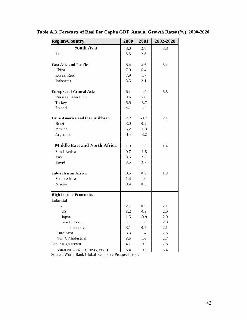
To project future vehicle ownership and traffic fatalities assumptions must be

made about income and population growth. The real per capita GDP series is projected

to 2020 using the World Bank’s forecasts of regional growth rates (2000-2010) (Global

Economic Prospects 2002) with the assumption that the average annual 2001-2010

growth rates continue to 2020. (A list of the growth rates is provided in Appendix Table

A.3.) Population projections are taken from the U.S. Census International Data Base. In

total, the explanatory variables are available for 156 countries (representing 92% of total

world population in 2000), including 45 highly developed countries (HD1) and 111

developing countries (HD2). Table 7 shows the number of countries in each geographic

region for which predictions are made.

25

Table 7. Regional Distribution of Countries for Which Predictions are Made

WB Region HD2 HD1

East Asia & Pacific 14 1 E. Europe & Central Asia 5 4 Latin America & Caribbean 27 4 Middle East & North Africa 12 1 South Asia 7 Sub-Saharan Africa 46 High-Income Countries 35

Total: 111 45

To calculate the point estimates for the out-of-sample countries, assumptions must

be made regarding the country-specific intercept. The coefficient on the country dummy

variable for Chile is used to compute the predicted values for the 10 out-of-sample HD1

countries.10 For the HD2 countries, the intercept is set equal to the mean of the country

intercepts for the corresponding region.

A. Projections of the World Vehicle Fleet to 2020

We begin by examining the implications of the models in Table 5 for future

growth in vehicle ownership. Figure 10 displays projections of the vehicle fleet

corresponding to all 8 models in Table 5. Not surprisingly, it is the form of the time

trend, rather than the choice between the spline and quadratic specifications, that makes

the greatest difference in the projections. Both the spline and quadratic models with

linear regional time trends yield unbelievably large estimates of the world motor vehicle

stock in 2020, as well as estimates of vehicle ownership per capita for certain groups of

countries that are well over 1. For this reason we focus on the spline models with log-

10 The choice of Chile is motivated by the fact that the most populous out-of-sample HD1 countries for which predictions must be made are Argentina and Uruguay.

26

linear time trends. The model with region-specific log- linear time trends (Model 8)

generates forecasts of 1.47 billion vehicles in 2020, whereas the vehicle stock is predicted

to be over 1.37 billion vehicles when a common log-linear time trend is used (Model 6).11

Figure 10. World Vehicle Fleet Projections Corresponding to Models in Table 5

The predictions of these models agree fairly well with other estimates of vehicle

growth in the literature. Dargay and Gately (1999) project that the total vehicle fleet in

OECD countries will reach 705 million by 2015 (a 62% increase from 1992 values). The

spline model (with the common time trend or the log- linear regional time trends) yields a

2015 estimate of 687 million vehicles for the same group of countries.

11 The corresponding quadratic models give almost identical vehicle projections but we continue to focus on the more flexible spline specifications.

0

500

1,000

1,500

2,000

2,500

3,000

3,500

1990 1995 2000 2005 2010 2015 2020

Num

ber

of V

ehic

les

(mill

ions

)

Model 1

Model 2Model 3Model 4

Model 5Model 6Model 7

Model 8

27

Other studies have made projections of vehicle growth for the automobile fleet

only or for passenger cars and commercial vehicles. Since our motor vehicle counts

include all buses and two-wheelers, direct comparisons with these studies is difficult.

However, our estimates of the total vehicle fleet do exceed their automobile forecasts

under all specifications. Under Schafer’s (1998) results, the global automobile fleet

would more than double from 470 million in 1990 (this includes light trucks for personal

travel in the U.S.) to 1.0-1.2 billion automobiles in 2020. This amounts to a 113%-155%

increase in total automobiles. The spline model with log-linear regional time trends

generates a 140% increase in the total vehicle fleet during the same period (from 609

million to 1.47 billion total vehicles). Because it yields reasonable predictions of the

vehicle fleet, as well as reasonable income elasticity estimates, we focus on the spline

model with regional, log- linear time trends.

B. Projections of World Traffic Fatalities to 2020

Figure 11 shows predictions of road traffic fatalities for all countries to the year

2020, based on the spline model with log- linear regional time trends. Ninety-five percent

confidence levels for our predictions also appear on the graph. 12 We emphasize that

these figures represent traffic fatalities unadjusted for under-reporting. To compare these

figures with fatality rates from other causes of death, it is necessary to adjust for the fact

that (a) the definition of what constitutes a traffic fatality differs across countries and (b)

the percentage of traffic fatalities reported by the police also varies across countries.

12The model generates point es timates of the log of the fatality rate (ln(Fatalities/10,000 People)). Therefore, the confidence intervals for the predicted values of ln(Fatalities/10,000 People) are symmetric, but the forecast intervals for the total number of fatalities are not.

28

Figure 11. Global Road Traffic Fatalities, Before Adjusting for Under-Reporting, 1990-2020

Our under-reporting adjustments follow the conservative factors used by Jacobs,

Aeron-Thomas and Astrop (2000).13 To update all point estimates to the 30-day traffic

fatality definition, a correction factor of 1.15 was applied in the developing countries and

the standard ECMT correction factors were used for the high- income countries.14 Then

the estimates were adjusted to account for general under-reporting of traffic fatalities, by

25% in developing countries and by 2% in highly developed countries.15 With these

adjustments, global road deaths are projected to climb to over 1.2 million by 2020 (a 40%

adjustment over the base estimate of 864,000 presented in Figure 11). Although this

13Jacobs et al. reviewed numerous underreporting studies and found evidence of underreporting rates ranging from 0-26% in high motorized countries and as high as 351% in less motorized countries. Fatalities in China, for example, were 42% higher in 1994 than reported in official statistics (Liren 1996). 14 High-Income countries with ECMT correction factors greater than 1 include: France: 1.057, Italy: 1.07, Portugal: 1.3, Japan: 1.3 (ECMT 1998, 2000, 2001). 15 The 25% under-reporting adjustment is applied to 111 HD2 countries and the 2% adjustment is used for 45 HD1 countries. See Table 7 for regional breakdown of countries.

0

200,000

400,000

600,000

800,000

1,000,000

1,200,000

1,400,000

1990 1995 2000 2005 2010 2015 2020

Estimated Number of Traffic FatalitiesLower Bound of 95% Forecast IntervalUpper Bound of 95% Forecast Interval

29

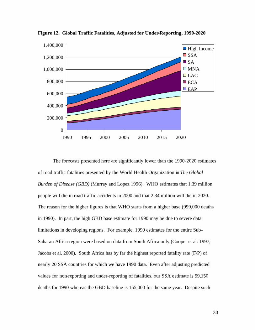
represents a 66% increase over the 2000 world estimate, the trend varies considerably

across different regions of the world. Table 8 and Figure 12 indicate that, between 2000

and 2020, fatalities are projected to increase by over 80% in developing countries, but

decrease by nearly 30% in high- income countries. Within the developing world, the

greatest percentage increases in traffic deaths between 2000 and 2020 will occur in South

Asia (144% increase), followed by East Asia and Sub-Saharan Africa (both showing an

80% increase). It is also interesting to note that the number of traffic fatalities per

100,000 persons is predicted to diverge considerably by 2020. By 2020 the fatality rate is

predicted to be less than 8 in 100,000 in high- income countries but nearly 20 in 100,000

in low-income countries.

Table 8. Predicted Road Traffic Fatalities by Region (000s), Adjusted for Under-Reporting, 1990-2020

Fatality Rate (Deaths/100,000

Persons)

Region* No. of

Countries 1990 2000 2010 2020 % change

'00-'20 2000 2020 EAP 15 112 188 278 337 79.8% 10.9 16.8 ECA 9 30 32 36 38 18.2% 19.0 21.2 LAC 31 90 122 154 180 48.1% 26.1 31.0 MNA 13 41 56 73 94 67.5% 19.2 22.3 SA 7 87 135 212 330 143.9% 10.2 18.9 SSA 46 59 80 109 144 79.8% 12.3 14.9

Subtotal: 121 419 613 862 1,124 83.3% 13.3 19.0

High Income Countries: 35 123 110 95 80 -27.8% 11.8 7.8

World Total: 156 542 723 957 1,204 66.4% 13.0 17.4 *The results are displayed according to the World Bank regional classifications.

30

Figure 12. Global Traffic Fatalities, Adjusted for Under-Reporting, 1990-2020

The forecasts presented here are significantly lower than the 1990-2020 estimates

of road traffic fatalities presented by the World Health Organization in The Global

Burden of Disease (GBD) (Murray and Lopez 1996). WHO estimates that 1.39 million

people will die in road traffic accidents in 2000 and that 2.34 million will die in 2020.

The reason for the higher figures is that WHO starts from a higher base (999,000 deaths

in 1990). In part, the high GBD base estimate for 1990 may be due to severe data

limitations in developing regions. For example, 1990 estimates for the entire Sub-

Saharan Africa region were based on data from South Africa only (Cooper et al. 1997,

Jacobs et al. 2000). South Africa has by far the highest reported fatality rate (F/P) of

nearly 20 SSA countries for which we have 1990 data. Even after adjusting predicted

values for non-reporting and under-reporting of fatalities, our SSA estimate is 59,150

deaths for 1990 whereas the GBD baseline is 155,000 for the same year. Despite such

0

200,000

400,000

600,000

800,000

1,000,000

1,200,000

1,400,000

1990 1995 2000 2005 2010 2015 2020

High IncomeSSASAMNALACECAEAP

31

large differences between our base estimates and theirs, Murray and Lopez predict that

global traffic fatalities will grow at approximately the same rate as the present

projections. (Fatalities grow by 62% between 2000 and 2020 according to WHO and by

66% according to our estimates (see Table 8).)

We believe that Murray and Lopez (1996) have over-estimated road traffic

fatalities and stand behind the estimates presented here. One reason for this is that our

estimate of fatalities in 2000 (723,439) agrees with the TRL estimate of global road

deaths for 1999 (Jacobs et al. 2000), i.e., 745,769 fatalities worldwide (low under-

reporting adjustment case). The TRL 1999 estimate is based on published 1996 data

from 142 countries updated to 1999 levels and adjusted for non-reporting and under-

reporting of fatalities. Since this seems to be the most comprehensive, bottom-up

approach to estimating the global road death toll to date, we feel that it is the most

appropriate estimate against which to compare our projections. Our prediction of traffic

fatalities in 2020 (1.2 million deaths worldwide) also lies within the range suggested by

TRL for 2020 (1 to 1.3 million deaths), although the latter is not based on a statistical

model.

V. Conclusions

The results presented above suggest that, if developing countries follow historic

trends, it will take many years for them to achieve the motor vehicle fatality rates of high-

income countries. Provided that present policies continue into the future, the traffic

fatality rate of India, for example, will not begin to decline until 2042.16 (The projected

16 This assumes the annual real per capita GDP growth rate of 3.87% and India’s log-linear time trend (from model 8) will continue into the future.

32

peak corresponds to approximately 24 fatalities per 100,000 persons prior to any

adjustment for underreporting but becomes 34 fatalities per 100,000 persons if we

maintain the underreporting adjustment factors chosen above.) This is primarily due to

the fact that India’s per capita income (in 1985 international dollars) was only $2,900 in

2000, whereas F/P peaks at a per capita income of approximately $8,600. Similarly, in

Brazil F/P will not peak until 2032, and the model projects over 26 deaths per 100,000

persons as far out as 2050.

In other developing countries, the traffic fatality rate will begin to decline before

2020 but F/P rates will still exceed the levels experienced in High-Income countries

today (which average about 11 fatalities per 100,000 persons). Malaysia, for example, is

estimated to have over 20 fatalities per 100,000 persons (after adjusting for

underreporting) in 2020. If 5.1% growth continues beyond 2020, F/P will reach 11.1 by

2033 (using the same under-reporting adjustment as above); however, if the growth rate

decreases to 2.5% after 2020, F/P will reach 11.0 only in 2049.

The predictions in this paper, and the estimates of the income levels at which

traffic fatality rates begin to decline, assume the policies that were in place from 1963

through 1999 will continue in the future. Clearly, this may not be the case. In many

developing countries fatalities per vehicle could be reduced significantly through

interventions that are not reflected in our data. For example, drivers of two-wheelers

could be required to wear white helmets, traffic calming measures could be instituted in

towns, and measures could be taken to separate pedestrian traffic from vehicular traffic.

Whether such measures should be undertaken depends, of course, on their costs and their

33

effectiveness. The purpose of this paper has been to increase awareness of the nature and

growing magnitude of the problem.

34

References

American Automobile Manufacturers Association. 1993. World Motor Vehicle Data 1993. Washington, D.C.: AAMA.

Bangladesh Bureau of Statistics. National Data Bank. http://www.bbsgov.org/ .

China Statistical Yearbook. (various years). State Statistical Bureau, People’s Republic of China.

Cooper, R.S., B. Osotimehim, J. Kaufman, and T. Forrester. 1998. Disease burden in sub-Saharan Africa: what should we conclude in the absence of data? The Lancet 351: 208-210.

Cross National Time Series Database (CNTS). Access through Rutgers University Libraries. http://www.scc.rutgers.edu/cnts/about.cfm .

Dargay, Joyce, and Dermot Gately. 1999. Income’s effect on car and vehicle ownership, worldwide: 1960-2015. Transportation Research A 33:101-138.

European Conference of Ministers of Transport. 2001. Statistical Report on Road Accidents 1997-1998. Paris: OECD Publications Service.



Grossman, Gene and Alan Krueger. 1995. “Economic Growth and the Environment.” Quarterly Journal of Economics 110(2): 675-708

Inter-American Development Bank. 1998. Review of Traffic Safety Latin America and Caribbean Region. Transport Research Laboratory and Ross Silcock.

International Road Federation. Various Years. I.R.F. World Road Statistics. Geneva, Switzerland: International Road Federation.

International Road Traffic Accident Database (IRTAD). Paris, France: Federal Highway Research Institute (BASt)/OECD Road Transport Research Programme.

Israel National Road Safety Authority. 2000. The National Road Safety Authority Structure, Activities, & Responsibilities. State of Israel Ministry of Transport.

Ingram, Gregory K., and Zhi Liu. 1998. Vehicles, Roads, and Road Use: Alternative Specifications. Working Paper 2036. World Bank.

Jacobs, G, A. Aeron-Thomas, and A. Astrop. 2000. Estimating Global Road Fatalities. TRL Report 445. London, England: Transportation Research Laboratory.

35

Liren, D. 1996. Viewing China Road Traffic Safety and the Countermeasures in Accordance with International Comparison. Beijing Research in Traffic Engineering, Second Conference in Asian Road Safety, 28-31 October 1996.

Murray, C. and A. Lopez (eds.). 1996. The Global Burden of Disease. Cambridge, MA: Harvard Press.

Road Safety in Latin America and the Caribbean: Analysis of the Road Safety Situation in Nine Countries. Copenhagen, Denmark: Ministry of Transport Road Directorate, 1998.

Schmalensee, Richard, Thomas M. Stoker, and Ruth A. Judson. 2000. World Carbon Dioxide Emissions: 1950-2050. Review of Economics and Statistics 80(1):15-27.

Schafer, Andreas. 1998. The Global Demand for Motorized Mobility. Transportation Research A 32(6):455-477.

Smeed, R. J. 1949. “Some Statistical Aspects of Road Safety Research.” Journal of the Royal Statistical Society Series A. 112:1-23.

Statistical Economic and Social Research and Training Centre for Islamic Countries (SESRTCIC). Basic Socio-Economic Indicators Database (BASEIND). http://www.sesrtcic.org/defaulteng.shtml.

United Nations Economic and Social Commission for Asia and the Pacific. 1997. Asia-Pacific Road Accident Statistics and Road Safety Inventory. New York: United Nations.

U.S. Census Bureau. International Data Base (IDB). http://www.census.gov/ipc/www/idbsprd.html

World Bank. Global Development Network Growth Database Macro Time Series. http://www.worldbank.org/research/growth/GDNdata.htm .

World Bank. Global Economic Prospects and the Developing Countries 2002. http://www.worldbank.org/prospects/gep2002/toc.htm

World Resources Institute. 1998-1999. World Resources. Washington, D.C. http://www.wri.org/wr-98-99/autos.htm.

36

VI. Appendix Data Sources

Data on the number of traffic fatalities and vehicle fleet17 composition were taken

from various editions of the International Road Federation’s (IRF) World Road Statistics

(WRS) annual yearbooks, 1968-2000. Since each WRS edition contains data for the

previous five years, each series was compared across editions to check for accuracy and

to ensure that all revisions were properly recorded. Selected IRF data were also

compared to numerous regional and country-specific road safety studies. Supplementary

data was added from several sources where appropriate, including studies published by

the

• Inter-American Development Bank (1998)

• Danish Road Directorate (1998)

• Transportation Research Laboratory (Jacobs et al. 2000)

• United Nations Economic and Social Commission for Asia and the Pacific

(1997)

• Statistical Bureau of the People’s Republic of China

• Ministry of Transport of Israel (2000)

• European Conference of Ministers of Transport (ECMT)

• Global Road Safety Partnership

• OECD International Road Traffic Accident Database (IRTAD)

• Cross-National Time Series Database (CNTS)

• Statistical Economic and Social Research and Training Centre for Islamic

Countries (SESRTCIC)

• Bangladesh Bureau of Statistics

• American Automobile Manufacturers Association

17 Vehicle counts include all passenger cars, buses, trucks, and motorized two-wheelers.

37

Population figures came from the U.S. Census Bureau’s International Data Base

and income data were taken from the World Bank Global Development Network Growth

Database Macro Time Series. The income variable most appropriate for this analysis is

the Real Per Capita GDP, chain method (1985 international prices) (RGDPCH), since it

accounts for differences in purchasing power across countries and allows for comparisons

over time.18

18 This series was created from the Penn World Tables 5.6 RGDPCH variable for 1960-1992 and the 1992-1999 data was estimated using the 1985 GDP per capita and GDP per capita growth rates from the Global Development Finance and World Development Indicators.

38

Table A.1. Classification of Countries for Which Fatalities Are Projected The number of observations for each country used to estimate the model is given in parentheses after the country name.

Region Country Region Country South Asia (SA) Latin America &Caribbean (LAC)

HD2:Bangladesh (18) HD1:Argentina Bhutan Chile (34) India (27) Costa Rica (14) Maldives Uruguay Nepal (14) HD2:Antigua & Barbuda Pakistan (33) Belize Sri Lanka (34) Bolivia Brazil (16)

East Asia & Pacific (EAP) Colombia (27)HD1:Korea, Rep. (29) Dominica HD2:China (22) Dom. Republic

Fiji (15) Ecuador (13) Indonesia (24) El Salvador Kiribati Grenada Lao PDR Guatemala Malaysia (37) Guyana Mongolia (14) Haiti Papua New Guinea (12) Honduras Philippines (18) Jamaica Samoa (13) Mexico Solomon Islands Nicaragua Thailand (28) Panama (16) Tonga (13) Paraguay Vanuatu Peru (11)

Puerto Rico

Middle East & N. Africa (MNA) St. Kitts & Nevis HD1:Bahrain (12) St. Lucia HD2:Algeria St. Vincent & Grenadines

Djibouti Suriname Egypt (11) Trinidad & Tobago Iran Venezuela Iraq (11)

Jordan (32) Europe & Central Asia (ECA) Morocco (34) HD1:Czech Republic (28) Oman Hungary (33) Saudi Arabia (20) Poland (19) Syria (22) Slovak Republic Tunisia (26) HD2:Bulgaria (18) Yemen (12) Georgia Latvia (11) Romania (13) Turkey (34) Yugoslavia (20)

39

(Table A.1. continued)

Sub-Saharan Africa (SSA) High-Income OECD

HD2:Angola HD1:Australia (31) Benin (23) Austria (37) Botswana (31) Belgium (36) Burkina Faso Canada (30) Burundi Denmark (37) Cameroon (17) Finland (37) Cape Verde France (37) Central African Republic Germany (30) Chad Greece (36) Comoros Iceland (35) Congo, Dem. Rep. Ireland (31) Congo, Rep. Italy (35) Cote d'Ivoire (17) Japan (37) Equatorial Guinea Luxembourg (34) Ethiopia (30) Netherlands (37) Gabon New Zealand (37) Gambia, The Norway (37) Ghana Portugal (37) Guinea Spain (32) Guinea-Bissau Sweden (35) Kenya (27) Switzerland (36) Lesotho (21) United Kingdom (35) Liberia United States (36) Madagascar

Malawi (28) Other High-Income Mali HD1:Bahamas Mauritania Barbados Mauritius (26) Bermuda Mozambique (12) Cyprus (30) Namibia Hong Kong (36) Níger (24) Israel (32) Nigeria (15) Kuwait Rwanda Malta Sao Tome &Principe Qatar Senegal (19) Singapore (16) Seychelles Taiwan (25) Sierra Leone (17) U.A.E. Somalia South Africa (35) Sudan Swaziland (13) Tanzania Togo (16) Uganda (19) Zambia (13) Zimbabwe (15) Total: 156 Countries, 2,178 Country-year Observations

40

Notes for Table A.2: Standard Errors are given in parentheses. The constant term reflects the intercept term for India. Country fixed effects were included in all regressions but are not displayed here.

Model Specifications:

1. Quadratic, common linear time trend 2. Quadratic, common log-linear time trend 3. Quadratic, regional linear time trends 4. Quadratic, regional, log- linear time trends 5. Spline, common linear time trend 6. Spline, common log- linear time trend 7. Spline, regional linear time trends 8. Spline, regional, log- linear time trends

41

Table A.2. Regression Results from Fatalities/Population Models Quadratic Spline Independent

Variables 1 2 3 4 5 6 7 8

lnY 7.7500* (0.2243)

7.8146* (0.2223)

5.1714* (0.3058)

6.1926* (0.2886)

(lnYit)2 -0.4510* (0.0137)

-0.4607* (0.0134)

-0.2785* (0.0191)

-0.3578* (0.0177)

lnY for: $1- $938

1.6837* (0.1432)

1.6067* (0.1434)

1.4445* (0.1400)

1.2526* (0.1439)

$938- $1,395 1.1798* (0.1266)

1.1445* (0.1258)

1.1193* (0.1322)

1.0604* (0.1283)

$1,395- $2,043 0.5064* (0.1219)

0.4277* (0.1209)

0.5119* (0.1250)

0.3256* (0.1278)

$2,043- $3,045 0.9199* (0.1304)

0.8177* (0.1302)

0.9757* (0.1299)

0.7651* (0.1345)

$3,045- $4,065 0.6995* (0.1526)

0.6221* (0.1520)

0.9602* (0.1492)

0.7007* (0.1495)

$4,065- $6,095 0.3225* (0.1146)

0.2758* (0.1130)

0.6021* (0.1119)

0.3903* (0.1107)

$6,095- $8,592 -0.0477 (0.1318)

-0.1119 (0.1315)

0.2579* (0.1288)

0.0746 (0.1299)

$8,592-$10,894 -0.7910* (0.1645)

-0.9382* (0.1658)

-0.2074 (0.1633)

-0.5422* (0.1668)

$10,894-13,234 -1.5720* (0.1952)

-1.6733* (0.1904)

-0.6682* (0.1999)

-1.3381* (0.1886)

>$13,234 -1.1509* (0.1637)

-1.2061* (0.1603)

-0.5216* (0.1637)

-0.9964* (0.1571)


$5,385 $4,825 $10,784 $5,738 $6,095 $6,095 $8,592 $8,592

95% C.I.: [$4977, $5826]

[$4489, $5186]

[$8644, $13455]

[$5141, $6403]


-0.0010 (0.0010)

0.0346* (0.0123)

0.0013 (0.0010)

0.0555* (0.0122)

Regional t: EAP

0.0054* (0.0029)

0.2377* (0.0417)

0.0065* (0.0029)

0.2573* (0.0416)

ECA -0.0100* (0.0032)

0.0162 (0.0399)

-0.0126* (0.0032)

-0.0305 (0.0403)

India 0.0194* (0.0048)

0.2789* (0.0591)

0.0225* (0.0048)

0.3189* (0.0579)

LAC 0.0145* (0.0032)

0.3100* (0.0625)

0.0120* (0.0032)

0.2639* (0.0615)

MNA -0.0093* (0.0023)

-0.0301 (0.0301)

-0.0067* (0.0025)

0.0106 (0.0324)

SA -0.0015 (0.0031)

0.0361 (0.0389)

0.0041 (0.0032)

0.0956* (0.0388)

SSA 0.0101* (0.0013)

0.1468* (0.0191)

0.0106* (0.0013)

0.1609* (0.0186)

High Income -0.0191* (0.0016)

-0.0783* (0.0177)

-0.0154* (0.0017)

-0.0567* (0.0176)


35.60 F8,2102 =

19.72 F8,2094=

29.50 F8,2094=

20.99

constant -32.948* (0.9128)

-33.046* (0.9092)

-23.796* (1.1952)

-27.427* (1.1416)

-12.550* (0.9606)

-12.149* (0.9596)

-11.359* (0.9360)

-10.462* (0.9599)


42

Table A.3. Forecasts of Real Per Capita GDP Annual Growth Rates (%), 2000-2020

Region/Country 2000 2001 2002-2020 South Asia 3.0 2.8 3.8

India 3.3 2.8 East Asia and Pacific 6.4 3.6 5.1 China 7.0 6.4 Korea, Rep. 7.9 1.7 Indonesia 3.5 2.1 Europe and Central Asia 6.1 1.9 3.3 Russian Federation 8.6 5.0 Turkey 5.5 -8.7 Poland 4.1 1.4 Latin America and the Caribbean 2.2 -0.7 2.1 Brazil 3.0 0.2 Mexico 5.2 -1.3 Argentina -1.7 -3.2

Middle East and North Africa 1.9 1.5 1.4

Saudi Arabia 0.7 -1.5 Iran 3.5 2.5 Egypt 3.5 2.7 Sub-Saharan Africa 0.5 0.3 1.3 South Africa 1.4 1.0 Nigeria 0.4 0.3 High-income Economies Industrial G-7 2.7 0.3 2.1 US 3.2 0.3 2.0 Japan 1.5 -0.9 2.0 G-4 Europe 3 1.3 2.3 Germany 3.1 0.7 2.1 Euro Area 3.3 1.4 2.5 Non-G7 Industrial 3.5 1.6 2.7 Other High-income 4.7 -0.7 2.8

Asian NIEs (KOR, HKG, SGP) 6.4 -0.7 3.4 Source: World Bank Global Economic Prospects 2002.

traffic fatalities and economic growth - … · 1 traffic fatalities and economic growth elizabeth...

Documents