trail formation ant - university of maryland · 1 introduction 2 acknowledgements: the authors wish...

Trail formation based on directed pheromone

deposition

Emmanuel Boissard(1,2) Pierre Degond(1,2)

Sebastien Motsch(3)

September 15, 2011

1-Université de Toulouse; UPS, INSA, UT1, UTM ;Institut de Mathématiques de Toulouse ;

F-31062 Toulouse, France.2-CNRS; Institut de Mathématiques de Toulouse UMR 5219 ;

F-31062 Toulouse, France.email: [email protected] ;

[email protected]

3-Center of Scientific Computation and Mathematical Modeling (CSCAMM);University of Maryland, College Park, MD 20742

email: [email protected]

Abstract

We propose an Individual-Based Model of ant-trail formation. The antsare modeled as self-propelled particles which deposit directed pheromones andinteract with them through alignment interaction. The directed pheromonesintend to model pieces of trails, while the alignment interaction translatesthe tendency for an ant to follow a trail when it meets it. Thanks to ade-quate quantitative descriptors of the trail patterns, the existence of a phasetransition as the ant-pheromone interaction frequency is increased can be ev-idenced. Finally, we propose both kinetic and fluid descriptions of this modeland analyze the capabilities of the fluid model to develop trail patterns. Weobserve that the development of patterns by fluid models require extra trailamplification mechanisms that are not needed at the Individual-Based Modellevel.

1 Introduction 2

Acknowledgements: The authors wish to thank J. Gautrais, C. Jost and G.Theraulaz for fruitful discussions. P. Degond wishes to acknowledge the hospitalityof the Mathematics Department of Tsinghua University where this research wascompleted. The work of S. Motsch is partially supported by NSF grants DMS07-07949, DMS10-08397 and FRG07-57227.

Key words: Self-propelled particles, pheromone deposition, directed pheromones,alignment interaction, Individual-Based Model, trail detection, pattern formation,kinetic models, fluid models

AMS Subject classification: 35Q80, 35L60, 82C22, 82C31, 82C70, 82C80,92D50.

1 Introduction

One of the many features displayed by self-organized collective motion of animalsor individuals is the formation of trails. For instance, ant displacements are charac-terized by their organization into lanes consisting of a large number of individuals,for the purpose of exploring the environment or exploiting its resources. Anotherexample involving species with higher cognitive capacities is the formation of moun-tain trails by hikers or herds of animals. In both cases, the main feature is thatthe interaction between the individuals is not direct, but instead, is mediated bya chemical substance or by the environment. Indeed, ants lay down pheromonesas chemical markers. These pheromones are sensed by other individuals which usethem to adjust their path. In the case of mountain trails, the modification of thesoil by walkers facilitates the passage of the next group of individuals and attractsthem. This phenomenon is well-known to biologists under the name of stigmergy, aconcept first forged by Pierre-Paul Grassé [20] to describe the coordination of socialinsects in nest building.

The formation of trails by ants has been widely studied in the biological lit-erature [1, 11, 13–15, 34]. One general observation is the fact that trail formationis a self-organized phenomenon and expresses the emergence of a large-scale orderstemming from simple rules at the individual level. Indeed, ant colonies in thenumbers of thousands of individuals or more arrange into lines without resortingto long-range signaling or hierarchical organization. Another striking feature is thevariability of the trail patterns, which may range from densely woven networks toa few large trails. This flexibility may result from the ability of the individuals toadapt their activity to variable external conditions such as food availability, tem-perature, terrain conditions, the presence of predators, etc. Trail plasticity derivesfrom internal and external factors: for example it may vary according to the speciesof ant under consideration or depends on the properties of the soil. Our goal is to

1 Introduction 3

provide a model that accounts for these two general facts: spontaneous formationof trails, and variability of the trail pattern.

At the mathematical level, several types of ant displacement and pheromonedeposition models have been introduced. A first series of works deal with antdisplacement on a pre-existing pheromone trail and focus on the role of the antennasin the trail sensing mechanism [6, 7, 11]. Spatially one-dimensional models do notspecifically address the question of trail build-up either, since motion occurs on aone-dimensional predefined trail. One-dimensional cellular automata models havebeen used to determine the fundamental diagram of pheromone-regulated trafficand to study the spontaneous break-up of bi-directional traffic in one preferreddirection [22, 24].

The decision-making mechanisms which lead to the selection of a particularbranch when several routes are available have been modeled by considering OrdinaryDifferential Equations (ODE’s) for the global ant and pheromone densities on eachtrail [2,12,19,28]. These models do not account for the spontaneous formation of thetrails. In [14], the spatial distribution of trails is ignored in a similar way. However,it introduces the concept of a space-averaged statistical distribution of trails, whichreveals to be very effective. In the present work, we have borrowed from [14] theidea of considering trails as particles in the same fashion as ants, and of dealing withthem through the definition of a trail distribution function. However, by contrastto [14], we keep track of both the spatial and directional distribution of these trails.

In general, two dimensional models consider that ant motion occurs on a fixedlattice. Two classes of ant models have been considered: Cellular Automata models[15, 17, 34], and Monte-Carlo models [2, 12, 29, 30, 32]. In the first class of models,no site can be occupied by more than one ant, while in the second class, ants aremodeled as particles subject to a biased random walk on the lattice. In [33], theauthors introduce some mean-field approximation of the previous models: a time-continuous Master equation formalism is used to determine the evolution of theant density on each edge. In all these models, the jump probabilities are modifiedby the presence of pheromones. The pheromones can be located on the nodes[29, 30, 32], but the trail reinforcement mechanism seems more efficient if they arelocated on the edges [2, 12, 15, 17, 34]. To enhance the trail formation mechanisms,some authors [30,32] introduce two sorts of pheromones, an exploration pheromonewhich is deposited during foraging and a recruit pheromone which is laid down byants who have found food and try to recruit congeners to exploit it. In [29], itis demonstrated that trail formation is enhanced by introducing some saturationof the ant sensitivity to pheromones at high pheromone concentrations. Inspiredby the observation that pheromone deposition on edges seems to be more efficientin producing self-organized trails, we suppose that laid down pheromones give riseto trails (i.e. directed quantities) rather than substance concentration (i.e. scalar

1 Introduction 4

quantities).All these previously cited two-dimensional models assume a pre-existing lattice

structure. One questions which is seldom addressed is whether this pre-existinglattice may influence the formation of the trails. For instance, it is well-knownthat lattice Boltzmann models with too few velocities have incorrect behavior. Onemay wonder if similar effects could be encountered with spatially discrete ant trailformation models. For this reason, in the present work, we will depart from a lattice-like spatial organization and treat the motion of the ants in the two-dimensionalcontinuous space.

In this work, we propose a time and space continuous Individual-Based Modelfor self-organized trail formation. In this model, self-propelled particles interact bylaying down pheromone trails that indicate both the position and direction of thetrails. Ants adapt their course by following trails deposited by others, thereforereinforcing existing trails while evaporation of pheromones allows weaker trails todisappear. The ant dynamics is time-discrete and is a succession of free flightsand velocity jumps occuring at time intervals ∆t. Velocity jumps occur with anexponential probability. Two kinds of velocity jumps are considered: purely randomjumps which translate the ability of ants to explore a new environment, and trail-recruitment jumps. In order to perform the latter, ants look for trails in a diskaround themselves, pick up one of these trails with uniform probability and adoptthe direction of the chosen trail.

This model bears analogies with chemotaxis models. Chemotaxis is the namegiven to remote attraction interaction through chemical signaling in colonies of bac-teria. Mathematical modeling of chemotaxis has been largely studied. Macroscopicmodels were first introduced by Keller and Segel in the form of a set of parabolicequations [23]. These equations can be obtained as macroscopic limits of kineticmodels [16, 18, 21, 25, 26]. Kinetic models describe the evolution of the populationdensity in position-velocity space. In [31] a direct derivation of the Keller-Segelmodel from a stochastic many-particle model is given. The common feature ofmost chemotaxis models is the appearance of blow-up, which corresponds to thefast aggregation of individuals at a specific point in space (see e.g. [4, 8]). By con-trast, in the present paper, the dynamics gives rise to the spontaneous organizationof lane-like spatial patterns, much alike to the observed behavior of ants. The rea-son for this different morphogenetic behavior is the directed nature of the mediatorof the interaction.

The model also bears analogies with the kinetic model of cell migration de-veloped in [27]. In this model, cells move in a medium consisting of interwovenextra-cellular fibers in the direction of one, randomly chosen fiber direction. Asthey move, cells specifically destroy the extracellular fibers which are transverseto their motion. The induced trail reinforcement mechanism produces a network.

2 An Individual-Based-Model of ant behavior 5

There are two differences with the trail formation mechanism that we present here.The first one is that the dynamics starts from a prescribed set of motion directionsand gradually reduces this set, while our algorithms builds up the set of availabledirections gradually and new directions are created through random velocity jumps.The second difference is the role of trail evaporation in our algorithm, which has noequivalent in the cell motion model. Indeed, trail evaporation is a major ingredientfor network plasticity.

In the last part of the present work, we derive a kinetic formulation of theproposed ant trail formation model in the spirit of [27]. Then, the fluid limit of thiskinetic model is considered. We show that the resulting fluid model can exhibittrail formation only if some concentration mechanism is involved, while numericalsimulations indicate that trail formation may occur without such a mechanism.Therefore, the appearance of trails is enhanced when the model provides moreinformation about the ant velocity distribution function.

The outline of this paper is as follows. In section 2, we provide the model descrip-tion. Section 3 is devoted to the analysis of the numerical simulations. We establisha methodology for the detection of trail patterns from a simulation outcome, and an-alyze the dependency of the observed features on the model parameters. In section4, we formally establish a set of kinetic equations that describes the dynamics andwe investigate their fluid limit. A conclusion in section 5 draws some perspectivesof this work.

2 An Individual-Based-Model of ant behavior

based on directed pheromone deposition

We consider N “ants” in a flat (2-dimensional) domain: each ant is described by itsposition xi ∈ R2 and the direction of its motion ωi. The vector ωi is supposed tobe of unit-length, i.e. ωi ∈ S1, where S1 denotes the unit circle. We also considerpieces of trails described by pairs (yp, ωp) where yp ∈ R2 is the trail piece positionand ωp is a unit vector describing the trail direction (see figure 1). In the caseof ants, the marking of the trail is realized by a chemical marker, namely a trailpheromone. We assume that the ants can distinguishably perceive the directionof the trail of this chemical marker and that they are able to follow, not the lineof steepest gradient, like in chemotaxis, but the direction of this trail. Note thatin the case of walkers or sheep in an outdoor terrain, the marking of the trail isrealized by the modification of the terrain consecutive to the passage of the walkers,such as flattened grass. For wild white bears, this modification is realized by thetrail left in the snow by the animals. In the sequel, we concentrate on the modelingof ant trail formation, and we will indistinguishably refer to these pieces of trails


as ’trails’ or ’trail pheromones’, or simply, ’pheromones’. The set of pheromonesvaries with time, since new pheromones are created by the deposition process andpheromones disappear after some time in order to model the evaporation process.We will denote by P(t) the set of pheromones at time t.

The simulated ants follow a random walk process. During free flights, Anti moves in direction ωi at a constant speed c, i.e. is subject to the differentialequation:

xi = cωi, ωi = 0, (2.1)

where the dots stand for time derivatives. This free motion is randomly interruptedby velocity jumps. When Ant i undergoes a velocity jump at time t, its velocitydirection before the jump ωi(t−0) is suddenly changed into a different one ωi(t+0).The jump times are drawn according to Poisson distributions. In practice, a timediscrete algorithm is used, with time steps ∆t. With such a discretization, a Poissonprocess of frequency λ is represented by an event occuring with probability 1−e−λ∆t

over this time step. There are two kinds of jumps: random velocity jumps and trailrecruitment jumps.

Random velocity jumps. In this case, ωi(t+0) differs from ωi(t−0) by a random angle

ε, i.e. (ωi(t − 0), ωi(t + 0)) = ε, where ε is drawn out of a Gaussian distributionp(ε) with zero mean and variance σ2, periodized over [0, 2π], i.e.

p(ε) dε =∑

n∈Z

1

(2πσ2)1/2exp

(

−(ε + 2nπ)2

2σ2

)

dε, ε ∈ [0, 2π].

The frequency of the Poisson process is constant in time and denoted by λr.

Trail recruitment jump. In this case, ωi(t+0), is picked up with uniform probabilityamong the directions ωp of the trail pheromones located in the ball BR(xi(t)) ofradius R centered at xi(t) (see figure 1). BR(xi(t)) is the ant detection region andR its detection radius. More precisely, defining the set

Si(t) = {p ∈ P(t) , |xp − xi(t)| ≤ R},

Ant i chooses an index p in Si(t) with uniform probability and sets

ωi(t + 0) = ωp. (2.2)

A variant of this mechanism involves a nematic interaction (i.e. the deposited trailshave no specific orientation). In this case, the new direction is defined by

ωi(t + 0) = ±ωp, such that (ωi(t + 0), ωp) is acute. (2.3)

The nematic interaction makes more biological sense, since it seems difficult toenvision a mechanism which would allow the ants to detect the orientation of a given


(xi, ωi)

R

(xp, ωp)

Figure 1: Ants follow a random walk process. Each ant is moving on a straight lineuntil it undergoes a random velocity jump (left) or a trail recruitment jump (right).In this picture, a trail pheromone is located in the disk centered at the ant locationwhen the jump occurs, and of given radius R.

trail. The use of a uniform probability to select the interacting pheromone can bequestioned. For instance, the choice of the trail pheromone p could be dependent on

the angle (ωi(t), ωp) like considered in [33], but in the present work we will discardthis effect. Ants may also preferably choose the largest trails indicated by a largeconcentration of pheromones in one given direction. This ’preferential choice’ willbe discussed in connection to the kinetic and fluid models in section 4 but discardedin the numerical simulations of the Individual-Based Model.

The frequency of the Poisson process is given by λpMi(t) where Mi(t) is thenumber of pheromones in the detection region of Ant i: Mi(t) = Card(Si(t)),and λp is the trail recruitment frequency per unit pheromone. The dependencyof the jump frequency upon the number of detected pheromones accounts for theobserved increase of the alignment probability with the pheromone density. Ofcourse, nonlinear functions of the pheromone density could be chosen as well. Forinstance, some saturation of the detection capability occurs at large pheromonedensities, such as investigated in [29]. This effect will also be discarded here. Wealso discard any consideration of the detection mechanism, such as discussed e.g.in [6, 7, 11].

During their walk, ants leave trail pheromones at a certain deposition rate νd.If at time t, ant i deposits a pheromone, a new pheromone particle is created atposition xi(t) with the direction ωi(t). Hence, we postulate that:

At deposition times t, a pheromone p is created with (xp, ωp) = (xi(t), ωi(t)).

Pheromones have a life-time Tp and remain immobile during their lifetime. In thiswork, pheromone diffusion is neglected. Pheromone deposition and evaporationtimes are modeled by Poisson processes: each ant has a probability νd per unit of

3 Simulations and results 8

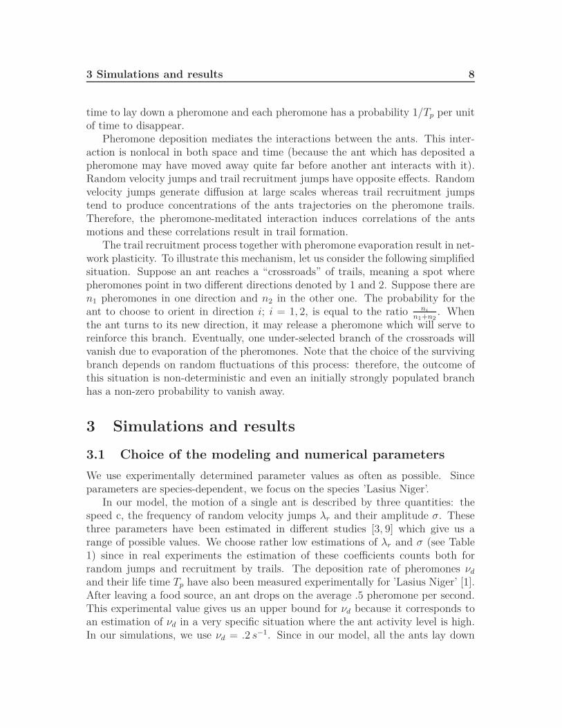
time to lay down a pheromone and each pheromone has a probability 1/Tp per unitof time to disappear.

Pheromone deposition mediates the interactions between the ants. This inter-action is nonlocal in both space and time (because the ant which has deposited apheromone may have moved away quite far before another ant interacts with it).Random velocity jumps and trail recruitment jumps have opposite effects. Randomvelocity jumps generate diffusion at large scales whereas trail recruitment jumpstend to produce concentrations of the ants trajectories on the pheromone trails.Therefore, the pheromone-meditated interaction induces correlations of the antsmotions and these correlations result in trail formation.

The trail recruitment process together with pheromone evaporation result in net-work plasticity. To illustrate this mechanism, let us consider the following simplifiedsituation. Suppose an ant reaches a “crossroads” of trails, meaning a spot wherepheromones point in two different directions denoted by 1 and 2. Suppose there aren1 pheromones in one direction and n2 in the other one. The probability for theant to choose to orient in direction i; i = 1, 2, is equal to the ratio ni

n1+n2

. Whenthe ant turns to its new direction, it may release a pheromone which will serve toreinforce this branch. Eventually, one under-selected branch of the crossroads willvanish due to evaporation of the pheromones. Note that the choice of the survivingbranch depends on random fluctuations of this process: therefore, the outcome ofthis situation is non-deterministic and even an initially strongly populated branchhas a non-zero probability to vanish away.

3 Simulations and results

3.1 Choice of the modeling and numerical parameters

We use experimentally determined parameter values as often as possible. Sinceparameters are species-dependent, we focus on the species ’Lasius Niger’.

In our model, the motion of a single ant is described by three quantities: thespeed c, the frequency of random velocity jumps λr and their amplitude σ. Thesethree parameters have been estimated in different studies [3, 9] which give us arange of possible values. We choose rather low estimations of λr and σ (see Table1) since in real experiments the estimation of these coefficients counts both forrandom jumps and recruitment by trails. The deposition rate of pheromones νd

and their life time Tp have also been measured experimentally for ’Lasius Niger’ [1].After leaving a food source, an ant drops on the average .5 pheromone per second.This experimental value gives us an upper bound for νd because it corresponds toan estimation of νd in a very specific situation where the ant activity level is high.In our simulations, we use νd = .2 s−1. Since in our model, all the ants lay down

3.1 Choice of the modeling and numerical parameters 9

Parameters ValueL Box size 100 cmN Number of ants 200c Ant speed 2 cm/sλr Random jump frequency 2 s−1

σ Random jump standard deviation .1νd Pheromone deposition rate .2 s−1

Tp Pheromone lifetime 100 sR Detection radius 1 cmλp Trail recruitment frequency 0-3 s−1

Table 1: Table of the parameters used in the simulations.

pheromones, we also take a low estimation of the pheromone lifetime (Tp = 100 s)otherwise the domain becomes saturated with pheromones.

By contrast, the interaction between ants and pheromones has not been quan-tified experimentally. For this reason, we do not have experimental values for thepheromone detection radius R and the alignment probability per unit of time λp.In our simulations, we fix the radius of perception R equal to 1 cm (correspondingroughly to 2 body lengths). The alignment probability λp remains a free param-eter in our model. By changing the value of λp, we can tune the influence of thepheromone-mediated interaction between the ants. A low value of λp correspondsto a weak interaction, whereas, for large values of λp, the ant velocities becomecontrolled by the pheromone directions. In our simulations, λp varies from 0 to3 s−1.

For simplicity, all simulations are carried out in a square domain of size L =100 cm with periodic boundary conditions. For the initial condition, 200 ants arerandomly distributed in the domain. Their velocity ωi is chosen uniformly on thecircle S1. The ant-pheromone interaction is always taken nematic unless otherwisestated.

We can estimate the average number of pheromones 〈M〉 at equilibrium, whenthe average is taken over realizations. The evolution of 〈M〉(t) is given by thefollowing differential equation:

d〈M〉(t)

dt= νdN −

1

Tp〈M〉(t),

where N is the number of ants, νd and Tp are (resp.) the deposition rate andpheromone lifetime. Thus, at equilibrium (i.e. d〈M〉/dt = 0), the average numberof pheromones is given by νd Tp N . For our choice of parameters (Table 1), thiscorresponds to 4000 pheromones.

3.2 Detection of trails 10

3.2 Detection of trails

3.2.1 Evidence of trail formation

The typical outcomes of the model are shown in figure 2. After an initial transient,we observe the formation of a network of trails. This network is not static, as weobserve in the two graphics: the network at time t = 2000 s is significantly differentfrom the network observed at time t = 1000 s. Here, the goal is to provide statisticaldescriptors of this trail formation phenomenon and to analyze it.

0

20

40

60

80

100

0 20 40 60 80 100

y

x

Ants and pheromones at t = 1000 s

0

20

40

60

80

100

0 20 40 60 80 100

y

x

Ants and pheromones at t = 2000 s

Figure 2: A typical output of the model at two different times. The ants arerepresented in blue and the pheromones in green. We clearly observe the formationof trails. Parameters of the simulation: λp = 2s−1, ∆t = .05 (see also Table 1).

3.2.2 Definition of a trail

To quantify the amount of particles that are organized into trails at a given time,we consider the collection of all particles, that is to say, the union of the sets ofants and of pheromones. Indeed collecting the pheromones allows us to trace backthe recent history of the individuals. To define a trail, we fix two parameters: adistance rmax and an angle θmax. We say that particle Pi = (xi, ωi) (Pi being eitheran ant or a pheromone) is linked to particle Pj = (xj , ωj) if the distance betweenthe two particles is less than rmax and the angle between ωi and ωj is either lessthan θmax or greater than π − θmax. In other words, we define a relationship (seefigure 3):

Pi ∼ Pj if and only if |xi − xj | < rmax and sin(ωj − ωi) < sin θmax. (3.1)


Using this relationship, particles can be sorted into different trails: we say thatP and Q belong to the same trail if there exists particles P1, . . . , Pk (a path) suchthat P ∼ P1, P1 ∼ P2, . . ., Pk ∼ Q. Thus, a trail is defined as the connectedcomponents of the particles under the relationship (3.1). A trail is approximatelya slowly turning lane of particles.

As a first example, in figure 4, we display the partitioning into trails of theprevious simulations (figure 2) at time t = 2000 s with rmax = 2 cm and θmax = 45◦.For these values, the largest trail (drawn in red in figure 4) consists of 2670 particlesand the second largest (drawn in orange in figure 4) is made of 254 particles.

3.2.3 Statistics of the trails

We expect that trail formation results in the development of a small number oflarge trails, while unorganized states are characterized by a large number of smalltrails, most of them being reduced to single elements. Therefore, trail formationcan be detected by observing the trail sizes. With this aim, we denote by Si(t) thesize of the trail to which particle i belongs at time t. Let N (t) be the total numberof particles, i.e. N (t) = N + P(t) where N is the number of ants and P(t) is thenumber of pheromones at time t. We form

pt(S) =Card({i | Si(t) = S})

N (t), S ∈ N.

pt(S) is the probability that a particle belongs to a trail of size S at time t. Anunorganized state is therefore characterized by a quickly decaying pt(S) as a functionof S while a state where the particles are highly organized into trails displays abimodal pt(S) with high values for large values of S. To display the distribution ofpt(S) is easy: it is nothing but the histogram of the trail sizes Si, collected fromseveral independent simulations with identical parameters.

As an illustration, we provide the distribution pt(S) for the set parameters usedto generate Figs. 2 and 4, (i.e. λp = 2 s−1, rmax = 2 cm and θmax = 45◦), with1000 realizations. We clearly observe in Fig. 5 (left) that the distribution pt(S) isbimodal: a first maximum is observed near the minimal value of S, i.e. S = 1, anda second maximum is observed near the values S ≈ 2500. This indicates that aparticle (i.e. an ant or a pheromone) belongs to either a small-size trail (S < 100) orto a large-size trail (S ≈ 2500). As a control sample for our statistical measurement,we run the same simulations but cutting off the ant-pheromone interaction (i.e.λp = 0) and proceed to the same analysis. In Fig. 5 (right), we observe thatwithout the influence of the pheromones (blue histogram) the probability pt(s) isonly concentrated near the value S = 1 and decays very fast to almost vanish forS > 500.


2

rmax

4

3

1

Figure 3: In this example, Ants 1, 2 and 3 are linked together: they form a trail.Ant 4 is not linked to Ant 2 since their directions are too different.

0

20

40

60

80

100

0 20 40 60 80 100

y

x

Two trails at t = 2000 s

Figure 4: The two largest trails (drawn in red and orange) for the simulation de-picted in figure 2 at time t = 2000 s. Parameters for the estimation of the trails:rmax = 2 cm and θmax = 45◦.

3.3 Trail size 13

0 500 1000 1500 2000 2500 3000 35000

1·105

2·105

3·105

4·105

Trail size S 0 500 1000 1500 2000 2500 3000 350002·105

4·105

6·105

8·105

10·105

12·105

λp = 2

λp = 0

Trail size SFigure 5: (Left) Histogram of the trail sizes S estimated from 1000 realizations.(Right) Histograms of S with and without trail-pheromone interaction (λp = 2 andλp = 0 resp.). The parameters for this simulation are the same as in Figs. 2 and 4.

3.3 Trail size

As observed in figure 5, ant-pheromone interactions lead to the formation of trailswhich are evidenced by the transformation of the shape of the distribution pt(S).To perform a systematic parametric analysis of the trail formation phenomenon, weuse the mean 〈S〉 of the distribution S:

〈S〉 =∑

S∈N

S pt(S).

The quantity 〈S〉 quantifies the level of organization of the system into trails. In-deed, large values of 〈S〉 indicate a high level of organization into trails while smallervalues of 〈S〉 are the signature of a disordered system. For example, in Fig. 5, wehave 〈S〉 = 1333.7 when the ant-pheromone interaction is on with interactionfrequency λp = 2. By contrast, its value falls down to 〈S〉 = 76.8 when the ant-pheromone interaction is turned off (i.e. λp = 0) and the system is in a fullydisordered state.

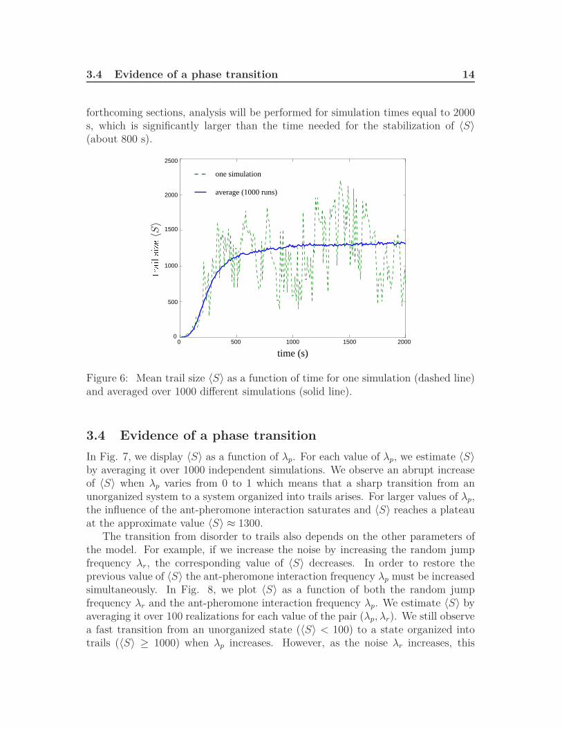
Our first use of the mean trail size 〈S〉 is to show that it stabilizes to a fixed valueafter an initial transient. Fig 6 shows the mean trail size 〈S〉(t) for one simulation(dashed line) and averaged over 1000 different simulations (solid line). It appearsthat, after some transient, 〈S〉(t) presents a lot of fluctuations about an averagedvalue. If the simulation is reproduced a large number of times and the mean trailsize 〈S〉(t) is averaged over all these realizations, the convergence towards a constantvalue becomes apparent.

Therefore, statistical analysis of the trail patterns using the mean trail size〈S〉 become significant only once this constant value has been reached. In the

3.4 Evidence of a phase transition 14

forthcoming sections, analysis will be performed for simulation times equal to 2000s, which is significantly larger than the time needed for the stabilization of 〈S〉(about 800 s).

0

500

1000

1500

2000

2500

0 500 1000 1500 2000

time (s)

average (1000 runs)

one simulation

trailsize〈S〉

Figure 6: Mean trail size 〈S〉 as a function of time for one simulation (dashed line)and averaged over 1000 different simulations (solid line).

3.4 Evidence of a phase transition

In Fig. 7, we display 〈S〉 as a function of λp. For each value of λp, we estimate 〈S〉by averaging it over 1000 independent simulations. We observe an abrupt increaseof 〈S〉 when λp varies from 0 to 1 which means that a sharp transition from anunorganized system to a system organized into trails arises. For larger values of λp,the influence of the ant-pheromone interaction saturates and 〈S〉 reaches a plateauat the approximate value 〈S〉 ≈ 1300.

The transition from disorder to trails also depends on the other parameters ofthe model. For example, if we increase the noise by increasing the random jumpfrequency λr, the corresponding value of 〈S〉 decreases. In order to restore theprevious value of 〈S〉 the ant-pheromone interaction frequency λp must be increasedsimultaneously. In Fig. 8, we plot 〈S〉 as a function of both the random jumpfrequency λr and the ant-pheromone interaction frequency λp. We estimate 〈S〉 byaveraging it over 100 realizations for each value of the pair (λp, λr). We still observea fast transition from an unorganized state (〈S〉 < 100) to a state organized intotrails (〈S〉 ≥ 1000) when λp increases. However, as the noise λr increases, this

3.5 Trail width 15

transition becomes smoother. Moreover, the plateau reached by 〈S〉 when λp islarge is still comprised between 1300 and 1500 for all values of λr, but reaching thisplateau for large values of λr requires larger value of λp.

At the value λr = 0, the transition from disorder (〈S〉 ≤ 100) to trail-likeorganization (〈S〉 ≥ 1000) is the fastest. However, the plateau reached by 〈S〉 whenλp is large is significantly lower than for larger values of λr (〈S〉 ≈ 1000 instead of1300). This could be attributed to the fact that, without random jumps, the level ofdiffusion is too low, the ants do not mix enough, and trails have little opportunitiesto merge.

On the other hand, we can look for another explanation of this paradoxicallower value of 〈S〉 when λr is very small. Indeed, we notice that, in this case, theformed trails are much narrower than for larger values of λr. Fig. 9 (left) showsa simulation result using a quite small random jump frequency of λr = .2. Weobserve that the trails are narrower and more straight than those obtained withthe larger value λr = 2 (figure 2). We can quantify statistically this feature bychanging the parameters of trail detection rmax and θmax. We reduce the maximumdistance (rmax = 1.5 cm) and the maximum angle (θmax = 35◦). With these smallervalues, two particles are less likely to be connected. Then we proceed to the sameanalysis as in figure 8, by estimating the mean size of the trails 〈S〉 as a functionof λr and λp, averaged over 100 realizations. As we observe in figure 9 (right), themean size of the trails 〈S〉 is much larger for smaller values of λr and we recover thesame behavior as that observed for larger values of λr. This discussion illustratesthe difficulty of working with an estimator which depends on arbitrary choices ofscales (here the space and angular threshold of trail detection). A discussion of thedependence of the trail width upon the biological parameters is developed in thenext section.

3.5 Trail width

A way to highlight the dependence of the trail width upon the model parameters isto compute a two-particle correlation distribution. Let a particle (ant or pheromone)i be located at position xi and velocity ωi. Denote by ω⊥

i the orthogonal vector toωi in the direct orientation. For all particles j 6= i, we form the vector

Xij =

(

(xj − xi) · ω⊥i

(xj − xi) · ωi

)

.

The distribution 2N (N −1)

f2(X), with

f2(X) = f2(Xx, Xy) =∑

(i,j), i6=j

δ(X − Xij),

3.5 Trail width 16

0

200

400

600

800

1000

1200

1400

0 0.5 1 1.5 2λp

〈S〉meantrailsize

〈S〉

Figure 7: The mean 〈S〉 of the distribution pt(s) as a function of the ant-pheromoneinteraction frequency λp for a fixed value of the random jump frequency λr.

0

0.5

1

1.5

2

2.5

3

0

0.5

1

1.5

2

2.5

30

500

1000

1500

2000

λp

λr

Mean trail size 〈S〉

Figure 8: The mean 〈S〉 of the distribution pt(s) as a function of the pair (λr, λp),The cuts of this surface at a fixed value of λr shows the same behavior as in figure7.

3.5 Trail width 17

0

20

40

60

80

100

0 20 40 60 80 100

y

x

Ants and pheromones with low noise

0

0.5

1

1.5

2

2.5

3

0

0.5

1

1.5

2

2.5

30

50

100

150

200

250

300

350

λp

λr

〈S〉 with rmax = 1.5 m and θmax = 35◦

Figure 9: (Left) A simulation with low noise (λr = .2); the other parameters are thesame as in figure 2 (t = 2000 s). (Right) The mean size of the trails 〈S〉 estimatedwith rmax = 1.5 cm and θmax = 35◦.

where δ is the Dirac delta, provides the probability that, given a first particle(located at say x0 with orientation ω0), a second particle lies at location x0+ω⊥

0 Xx+ω0Xy (see figure 10 (left) for an illustration of the construction of f2). Looking atthis 2-particle density, trails appear as concentrations near a line passing throughthe origin and directed in the y-direction. Figure 10 (right) provides a histogramof the two-particle density f2 for the simulation corresponding to the right pictureof fig. 2. The above mentioned concentration is clearly visible. Additionally, thetypical width of this concentration gives access to the typical width of the trails.

In order to better estimate the typical width of the trails, we plot cuts of thetwo-particle density f2 along the line {y = 0} (see figure 10). In practice, these cutsare determined by computing the following density

f2(r) =∑

(i,j), i6=j, |(Xij)y |≤ξ

δ(r − |(Xij)x|).

where ξ is suitable chosen (of the order of 1 cm). Figure 11 (left) displays f2(r) asa function of r for different values of the trail recruitment frequency λp and a fixedvalue of the random jump frequency equal to λr = 2 s−1. It appears that f2 is higherand decreases faster for larger values of λp. The decay of f2 can give an estimate ofthe width of the trail: if we approximate the decay of f2 by an exponential,

f2(r) ≈ f0 exp(

−r

r0

)

for r ≈ 0,

then r0 measures the typical width of the trail. This quantity can be estimated

4 Kinetic and continuum descriptions 18

using the formula:

r0 =1

|(ln f2)′(0)|. (3.2)

As we observe in Table 2, the width r0 increases as λp decreases. Therefore, in-creasing the trail recruitment frequency increases the intensity of the particles in-teractions and produces trails with smaller width. Figure 11 (right) displays f2(r)as a function of r for different values of the random jump frequency λr and a fixedvalue of the trail recruitment frequency equal to λp = 2 s−1. Here, the trail widthr0 estimated from f2 is larger for large values of λr (see Table 2), indicating thatthe typical width of the trails increases with increasing λr, as it should.

We also observe a discontinuity at r = 0 for all the functions f2 (figure 11).These jumps are easily explained by the deposit process: each time an ant dropsa pheromone, the new pheromone and the ant are located at the same positionexactly. This results in a peak of concentration of f2 at r = 0.

λp r0 (cm)3 2.7962 3.1811 4.350

λr r0 (cm)0 2.5321 2.9642 3.1813 3.345

Table 2: Estimations of the width r0 (3.2) of the trails using f2 given in figure 11.We estimate the derivative of ln f2(r) near 0 using the values of r between .1 and 2.

4 Kinetic and continuum descriptions

4.1 Framework

In this section, we propose meso- and macro-scopic descriptions of the previouslydiscussed ant dynamics. We first propose a kinetic model, i.e. a model for theprobability distributions of ants and pheromones. The derivation of this kineticmodel is formal and based on analogies with the underlying discrete dynamics. Arigorous derivation of the kinetic model from the discrete dynamics is up to nowbeyond reach. Issues such as the validity of the chaos propagation property [10],which is the key for proving such results, may be quite difficult to solve. Then, fluidlimits of this kinetic model will be considered. We will notice that the resulting fluidmodels can only exhibit the development of trails if some concentration mechanismis added, while the numerical simulations above indicate that such a mechanism isnot needed at the level of the Individual-Based Model.

4.1 Framework 19

$bidule$

{y = 0}x0

ω0

Xij

0.4

0.5

0.6

0.7

0.8

0.9

1Particle density

−4 −3 −2 −1 0 1 2 3 4−4

−3

−2

−1

0

1

2

3

4

lateralfr

ont

Figure 10: (Left) Construction of the two-particle distribution f2. (Right) His-togram of the two-particle density f2 for the test-case corresponding to the rightpicture of fig. 2. f2(X) is represented via a color scale as a function of the twocomponents of X.

0

0.5

1

1.5

2

0 1 2 3 4 5 6 7 8lateral distan e r ( m)

radial density f2 (λr = 2)λp = 3

λp = 0

λp = 2

λp = 1

0

0.5

1

1.5

2

0 1 2 3 4 5 6 7 8lateral distan e r ( m)

radial density f2 (λp = 2)λr = 0

λr = 1

λr = 2

λr = 3

Figure 11: (Left) f2(r) as a function of r for different values of the trail recruitmentfrequency λp and a fixed value of the random jump frequency equal to λr = 2 s−1.(Right) f2(r) as a function of r for different values of the random jump frequencyλr and a fixed value of the trail recruitment frequency equal to λp = 2 s−1.

4.2 Kinetic model 20

4.2 Kinetic model

In this section, we introduce the kinetic model of the discrete ant-pheromone in-teraction on a purely formal basis. We introduce the ant distribution functionF (x, ω, t) and the pheromone distribution function G(x, ω, t), for x ∈ R2, ω ∈ S1

and t ≥ 0. They are respectively the number density in phase-space (x, ω) of theants (respectively of the pheromones), i.e. the number of such particles located atposition x with orientation ω at time t. Here, we remark that the consideration ofdirected pheromones requires the introduction of a pheromone density in (position,orientation) phase-space in the same manner as for the ants.

Trail dynamics. The trail dynamics is described by the ordinary differentialequation:

∂tG(x, ω, t) = νdF (x, ω, t) − νeG(x, ω, t), (4.1)

This equation can be easily deduced from the evolution of the probability densityof the underlying stochastic Poisson process. The first term describes depositionby the ants according to a Poisson process of frequency νd while the second termresults from the finite lifetime expectancy Tp = ν−1

e of the pheromones. Pheromonesare supposed immobile, which explains the absence of any convection or diffusionoperator in this model. Discarding pheromone diffusion is done for simplicity onlyand can be easily added. It would add a term ∆xG or ∆ωG at the right-hand sideof (4.1) according to whether one considers spatial or orientational diffusion.

Ant dynamics. The evolution of the ant distribution function is ruled by thefollowing kinetic equation:

∂tF + c ω · ∇xF = Q(F ). (4.2)

The left-hand side describes the ant motion with constant speed c in the direction ω.The right hand side is a Boltzmann-type operator which describes the rate of changeof the distribution function due to the velocity jump processes. Q is decomposedinto

Q = Qr + Qp,

where Qr and Qp respectively describe the random velocity jumps and the trailrecruitment jumps.

Both operators Qk(x, ω, t), k = p or r express the balance between gain and lossdue to velocity jumps, i.e. Qk(x, ω, t) = Q+

k − Q−k . The gain term Q+

k describesthe rate of increase of F (x, ω, t) due to particles which have post-jump velocity ωand pre-jump velocity ω′. Similarly, the loss term Q−

k describes the rate of decayof F (x, ω, t) due to particles jumping from ω to another velocity ω′. The jumpprobability Pk(ω → ω′)dω′ is the probability per unit time that a particle with


velocity ω jumps to the neighborhood dω′ of ω′ due to jump process k. Therefore,the expression of Qk is:

Qk(F )(x, ω, t) =∫

S1

(

Pk(ω′ → ω)F (x, ω′, t) − Pk(ω → ω′)F (x, ω, t))

dω′. (4.3)

where the positive term corresponds to gain and the second term, to loss. Bysymmetry, we note that

∫

S1

Qk(F )(x, ω, t) dω = 0, (4.4)

for any distribution F . This expresses that the local number density of particles ispreserved by the velocity jump process.

Now we describe the expressions of the jump probabilities Pk. For both pro-cesses, we postulate the existence of a detailed balance principle, which means thatthe ratio of the direct and inverse collision probabilities are equal to the ratios ofthe corresponding equilibrium probabilities

Pk(ω′ → ω)

Pk(ω → ω′)=

hk(ω)

hk(ω′), (4.5)

where hk is the equilibrium probability of the process k (k = r or k = p). Using(4.5), we can define:

Φk(ω′, ω) =1

hk(ω)Pk(ω′ → ω) = Φk(ω, ω′),

which is symmetric by exchange of ω and ω′ and write

Qk(F )(x, ω, t) =∫

S1

Φk(ω, ω′)(

hk(ω) F (x, ω′, t) − hk(ω′) F (x, ω, t))

dω′. (4.6)

From this equation, it is classically deduced that the equilibria, i.e. the solutionsof Qk(F ) = 0 are given by F (x, ω, t) = ρ(x, t)hk(ω) with arbitrary ρ. We recall theargument here for the sake of completeness. Indeed, such F are clearly equilibria.Reciprocally, if F is an equilibrium, then, using the symmetry of Φk leads to

0 =∫

S1

Qk(F )F

hk

dω

= −1

2

∫

(S1)2

Φk(ω, ω′) hk(ω) hk(ω′)

(

F (x, ω′, t)

hk(ω′)−

F (x, ω, t)

hk(ω)

)2

dω dω′.

The last expression is the integral of a non-negative function which therefore mustbe identically zero for any choice of (ω, ω′). It follows that the only equilibriaare functions of the form ρhk with ρ only depending on (x, t). It is not clear if


the biological processes actually do satisfy the detailed balance property but thishypothesis simplifies the discussion. Indeed, with this assumption, the equilibria hk

and the jump probabilities Φk can be specified independently.

Trail recruitment jumps. For trail recruitment, we first need to specify theequilibrium distribution as a function of the pheromone distribution. Several op-tions are possible: non-local interactions, local ones, preferential choice, nematicinteractions.

1. Non-local interaction. We first introduce the sensing application:

SR(x, ω, t) =1

πR2

∫

|x−y|<RG(y, ω, t)dy,

where R represents the perception radius of the particle, i.e. the maximal distanceat which it can feel a deposited pheromones. The quantity SR(x, ω, t) representsthe density of pheromones pointing towards ω which can be perceived by an ant atpoint x in its perception area. We also define

TR(x, t) =∫

S1

SR(x, ω, t) dω,

the pheromone total density within the perception radius, regardless of orientation.Then, we let the equilibrium distribution of the trail recruitment process as follows:

hp(ω) = gR(x, ω, t) :=SR(x, ω, t)

TR(x, t), (4.7)

which, by construction, is a probability density. Now, The expression for the tran-sition probability reads:

Φp(ω → ω′; x, t) = λpγ(TR(x, t))φp(ω · ω′), (4.8)

where λp is the trail-recruitment frequency and γ is a dimensionless increasingfunction of T which accounts for the fact that recruitment by trails increases withpheromone density (in the discrete particle dynamics, we have taken γ(T ) = πR2T ,the total number of pheromones in the sensing region). The function φp(ω · ω′)represents the angular dependence of the interaction process and is such that

1

2π

∫

S1

φp(ω · ω′) dω′ = 1. (4.9)

We assume that it is independent of the pheromone distribution for simplicity.Inserting (4.8) into (4.6), the trail-recruitment operator is written:

Qp(F )(x, ω, t) = λpγ(TR(x, t))∫

S1

φp(ω · ω′)(gR(ω) F (x, ω′, t)

−gR(ω′) F (x, ω, t))dω′. (4.10)


The choice of φp which corresponds to the discrete dynamics discussed in the previ-ous sections is φp(ω · ω′) = 1. Inserting this prescription into (4.10) and using (4.7)leads to the simplified operator

Qp(F )(x, ω, t) = λpγ(TR(x, t))

(

ρ(x, t)SR(x, ω, t)

TR(x, t)− F (x, ω, t)

)

,

withρ(x, t) =

∫

F (x, ω, t)dω,

the local ant density at x.

2. Local interaction. This corresponds to taking the limit of the sensing radius tozero: R → 0 which leads to

hp(ω) = g(ω) :=G(x, ω, t)

T (x, t), T (x, t) =

∫

S1

G(x, ω, t) dω.

T is the local trail density. Then, the expression of the collision operator is easilydeduced from (4.10) by changing gR into g. In the case where φp = 1, we get theexpression:

Qp(F )(x, ω, t) = λpγ(T (x, t)) (ρ(x, t)g(x, ω, t) − F (x, ω, t)) .

3. Preferential choice. We can envision a mechanism by which the ants can senseand choose the most frequently used trails. A possible way to model this preferentialchoice is by postulating an equilibrium distribution of the form

hp(ω) = g[k]R (ω) =

gkR(ω)

∫

S1 gkR(ω) dω

, (4.11)

with a power k > 1. Indeed, it can be shown [5] that the maxima of g[k]R are larger

than those of gR and similarly, the minima are lower. Additionally, the monotonyis preserved, i.e.

gR(ω) ≤ gR(ω′) =⇒ g[k]R (ω) ≤ g

[k]R (ω′), ∀(ω, ω′) ∈ (S1)2.

Therefore, taking g[k]R (ω) as equilibrium distribution of the ant-pheromone interac-

tion means that the ants choose the trails ω with a higher probability when thetrail density in direction ω is high and with lower probability when the trail densityis low. The expression of the collision operator is easily deduced from (4.10) by

changing gR into g[k]R . In the case where φp = 1, we get:

Qp(F )(x, ω, t) = λpγ(TR(x, t))(

ρ(x, t)g[k]R (x, ω, t) − F (x, ω, t)

)

.


This mechanism can also be combined with a local interaction, by replacing gR

by the local angular pheromone probability g. We note that this mechanism isnot implementable in the discrete dynamics because the operation g → g[k] is onlydefined for measures g which belong to the Lebesgue space Lk(S1). However, sumsof Dirac deltas, which correspond to the measure g in the Individual-Based Model,do not belong to this space. Therefore, a smoothing procedure must be appliedto such measures beforehand. Since, it is not possible to obtain experimental dataabout the smoothing procedure and the power k, the preferential choice model hasnot been used in the numerical experiments of the previous sections.

4. Nematic interaction. The above described ant-pheromone interactions are polarones, i.e. the pheromones are supposed to have both a direction and an orientation.However, we can easily propose a nematic interaction, for which an ant of velocityω chooses ω′ among the pheromone directions and their opposite in such a way that

the angle (ω, ω′) is acute, i.e. such that ω · ω′ > 0. For this purpose, we modify theequilibria of the trail recruitment operator as follows:

hp(x, ω, t) = g(sym)R :=

SR(x, ω, t) + SR(x, −ω, t)

2TR(x, t),

and suppose thatφp(ω · ω′) = 0, when ω · ω′ ≤ 0. (4.12)

The expression of the collision operator is easily deduced from (4.10) by making the

change of gR into g(sym)R and imposing the restriction (4.12). In the case where

φp(ω · ω′) = 2H(ω · ω′),

where H is the Heaviside function (i.e. the indicator function of the positive realline), we find

Qp(F )(x, ω, t) = λpγ(TR(x, t))

[

1

TR(x, t)

(

ρ+ω (x, t) SR(x, ω, t)+

+ρ−ω (x, t) SR(x, −ω, t)

)

− F (x, ω, t)

]

,

withρ±

ω (x, t) =∫

F (x, ω′, t) H(±ω · ω′) dω′,

is the local density of ants pointing in a direction making respectively an acuteangle (for ρ+

ω ) or obtuse angle (for ρ−ω ) with ω at x.

Random velocity jumps. For random velocity jumps, we assume a uniformequilibrium

hr(ω) =1

2π,

4.3 Macroscopic model 25

with a given jump probability

Φr(ω, ω′) = λr φr(ω, ω′).

Here, φr satisfies the same normalization condition (4.9) as the trail recruitmentjump transition probability and λr is the random velocity jump frequency. With(4.6), we find the expression of Qr:

Qr(F ) = λr

(

∫

φr(ω.ω′)F (x, ω′, t)dω′

2π− F (x, ω, t)

)

.

If φr = 1, then Qr reduces to

Qr(F ) = λr

(

ρ(x, t)

2π− F (x, ω, t)

)

.

Summary of the kinetic model. Below, we collect all equations of the kineticmodel. We have written the model in the framework of non-local interaction, pref-erential choice and nematic interaction. The restriction to simpler rules is easilydeduced.

∂tG(x, ω, t) = νdF (x, ω, t) − νeG(x, ω, t), (4.13)

∂tF + c ω · ∇xF = Qr(F ) + Qp(F ), (4.14)

Qp(F )(x, ω, t) = λpγ(TR(x, t))∫

S1

φp(ω, ω′)(

hp(ω) F (x, ω′, t)

−hp(ω′) F (x, ω, t))

dω′, (4.15)

Qr(F )(x, ω, t) = λr

∫

S1

φr(ω, ω′)(

F (x, ω′, t) − F (x, ω, t))

dω′, (4.16)

hp(ω) = (g(sym)R )[k](ω), g

(sym)R (x, ω, t) =

SR(x, ω, t) + SR(x, −ω, t)

2TR(x, t), (4.17)

SR(x, ω, t) =1

πR2

∫

|x−y|<RG(y, ω, t)dy, TR(x, t) =

∫

S1

SR(x, ω, t) dω. (4.18)

In the following section, we consider fluid limits of the present kinetic model.

4.3 Macroscopic model

Scaling. In order to study the macroscopic limit of the kinetic model (4.13)-(4.18),we use the local interaction approximation R = 0, with non-nematic interaction anduniform transition probabilities φr = 1, φp = 1. In this case, the model simplifies


into

∂tG = νd F − νe G, (4.19)

∂tF + c ω · ∇xF = Qr(F ) + Qp(F ), (4.20)

Qp(F ) = λp γ(T ) [ρ h − F ] , (4.21)

Qr(F ) = λr

(

ρ

2π− F

)

, (4.22)

h = g[k], g =G

T, T =

∫

S1

G dω, ρ =∫

S1

F dω, (4.23)

where the meaning of the power [k] operation has been defined at (4.11). We nowchange to dimensionless variables. We let t0, x0, ρ0, T0, be respectively units of time,space, ant density and pheromone density and we introduce x′ = x/x0, t′ = t/t0,ρ′ = ρ/ρ0, T ′ = T/T0, F ′ = F/ρ0, G′ = G/T0 as new variables and unknowns.Specifically, t0 is chosen to be the macroscopic time scale (e.g. the observation timescale). Similarly, x0 is the macroscopic length scale (e.g. the size of the experimentalarena). We impose x0 = ct0, so that the time and space derivatives in (4.20) are ofthe same orders of magnitude. This scaling allows us to observe the system at theconvection scale where the convection speed of the ant density is finite.

We introduce the following dimensionless parameters:

νd = νd t0, νe = νe t0T0

ρ0, λp = λp t0, λr = λr t0.

We make the assumption that the macroscopic time scale t0 is very large comparedto the microscopic time scales λ−1

r and λ−1p which are both supposed to be of the

same orders of magnitude. Indeed, during the time needed for patterns to develop,ants make a large number of jumps of either kind. Following this assumption, weintroduce:

ε =1

λp

=1

λpt0≪ 1, σ =

λr

λp

=λr

λp= O(1).

Concerning the pheromone dynamics, we assume that νd and νe are of the sameorders of magnitude, which amounts to supposing that pheromone deposition andevaporation balance each other. Indeed, if one of these two antagonist phenomenapredominates, then, after some transient the pheromone density will become eithertoo low or too large and we cannot expect any interesting patterns to emerge inthis case. We introduce

η =1

νd=

1

νd t0, κ =

νe

νd=

νe

νd= O(1).

In what follows, we will assume that η = O(1) i.e. that the pheromone dynamicsoccurs at the macroscopic time scale.


After rescaling, system (4.19)-(4.23) becomes (dropping the primes for the sakeof clarity):

η ∂tGε = F ε − κ Gε, (4.24)

ε (∂tFε + ω · ∇xF ε) = Q(F ε), (4.25)

with the collision operator Q = Qr + Qp given by

Q(F ) = (Qr + Qp)(F ) = (γ(T ) + σ) (µ ρ − F ), (4.26)

µ =γ(T )h + σ

2π

γ(T ) + σ, h = g[k], g =

G

T, (4.27)

T =∫

S1

G dω, ρ =∫

S1

F dω. (4.28)

Macroscopic limit ε → 0 of the kinetic model (4.24)-(4.28). Here, wesuppose that η = O(1) i.e. we assume that the pheromone dynamics occurs atthe macroscopic scale. We show that the limit ε → 0 of (4.24)-(4.28) consistsof the following system for the ant density ρ(x, t), pheromone density T (x, t) andpheromone distribution function g(x, ω, t):

∂tρ + ∇x ·

(

γ(T )

γ(T ) + σjh

)

= 0., (4.29)

η∂tT = ρ − κT, (4.30)

η∂tg =ρ

T

(

γ(T )g[k] + σ2π

γ(T ) + σ− g

)

, (4.31)

with h = g[k] and where jϕ =∫

S1 ϕ(ω) ω dω, denotes the flux of any function ϕ(ω).Eq. (4.31) is a closed equation for g. Once g is determined and inserted into (4.29)the evolution of the ant density ρ can be computed. The ant distribution functionf is equal to µ at any time, with µ given by (4.27).

Indeed, in this limit, supposing that F ε → F , we get Q(F ) = 0 from (4.25).Therefore, from (4.26), we obtain

F = ρµ, or f = µ. (4.32)

The equation for ρ(x, t) is obtained by integrating (4.25) with respect to ω andusing (4.4). We find:

∂tρ + ∇x · jF = 0.

Remarking that jF = ρjµ and that the flux of the isotropic distribution vanishes,we finally get from (4.27):

jµ =γ(T )

γ(T ) + σjh, (4.33)


and consequently, ρ satisfies (4.29). To compute the pheromone distribution func-tion g, we integrate (4.24) with respect to ω and get (4.30). Then, combining (4.30)with (4.24), we deduce that

η∂tg =ρ

T(f − g). (4.34)

But, with (4.32) and (4.27), we deduce that g satisfies (4.31).Some comments are now in order. In the limit ε → 0 the ant distribution

function instantaneously relaxes to the distribution µ. This distribution reflects theantagonist effects of trail recruitment and random velocity jumps. Indeed, µ is theconvex combination of the equilibrium distributions h and 1

2πof the two processes

respectively. The weights, respectively equal to γ(T )/(γ(T ) + σ) and σ/(γ(T ) + σ)show that the influence of the trail recruitment process is more pronounced at largepheromone densities, since γ increases with T . On the other hand, if the frequencyof random jump σ is increased, the trail recruitment process is comparatively lessimportant.

Case k = 1: no preferential choice. If the ants do not implement a preferentialchoice of the largest trails, i.e. if k = 1, eq. (4.31) simplifies into

η∂tg =ρ

T

σ

γ(T ) + σ

(

1

2π− g

)

. (4.35)

This is a classical relaxation equation of g towards the isotropic distribution 12π

.As a consequence, in this case, there is no trail formation and the large time be-havior of the system leads to a homogeneous steady state. This description can becomplemented by looking at the pheromone flux jg. Indeed, (4.35) leads to

η∂tjg = −ρ

T

σ

γ(T ) + σjg.

As a consequence, the direction of the local pheromone flux never changes and itsintensity decays to 0 as t → ∞. Additionally, eq. (4.33) which in the case k = 1

gives jµ = γ(T )γ(T )+σ

jg shows that the ant flux is always proportional to and smallerthan the pheromone flux. Therefore, it also converges to 0 for large times. Note thatthis direction may not correspond to the maximum of the pheromone distributiong. Therefore, the ant flux may not be aligned with any particular trail, defined assuch a maximum.

The ant distribution µ is just the convex combination of the pheromone dis-tribution g and of the isotropic distribution. Therefore, the ant distribution isalways smoother than the pheromone distribution. The random velocity jump pro-cess, even if very weak, seems to prevent a positive feedback between the ant andpheromone distributions which could lead to the formation of trails. Of course,these conclusions hold only when ε → 0, i.e. if the equilibrium of the ant jump

5 Conclusion 29

operator is instantaneously reached. The fact that the simulations do indeed showthe formation of trails without any implementation of a preferential choice seems toindicate that the fast microscopic dynamics plays an important role in the forma-tion of trails which the macroscopic model is unable to capture. We also note that ifσ = 0, the pheromone distribution is constant in time. This is due to the fact that,in the absence of random velocity jumps, newly created pheromones are depositedaccording to a distribution which coincides exactly with the current pheromone dis-tribution, resulting in an exact zero balance for this distribution. Therefore, evenif σ = 0, no trails can develop.

Case k > 1: existence of a preferential choice. In this case, Eq. (4.31) is anon-local equation due to the operator g → g[k]. No analysis is available yet (toour knowledge) for such an equation (some preliminary results can be found in [5]).The large-time behavior of the system depends on the limit as t → ∞ of eq. (4.31).We note that (4.31) may produce concentrations [5]. Indeed, the contribution ofthe largest trails is amplified and the ant flux becomes more strongly correlatedto the direction of the largest trails. Therefore if the ants choose preferably thelargest trail, the resulting concentration dynamics may counterbalance the effectof the random velocity jumps and a positive feedback between the ants and thepheromones is more likely to occur. The study of this case is deferred to futurework.

Conclusion on macroscopic models. We have shown that macroscopic modelsare unable to develop trail formation without some mechanism allowing to amplifythe variations of the pheromone distribution function. We have provided an exampleof such a mechanism, referred to as the preferential choice and which consists forthe ants to choose the strong trails with higher probability than the weak ones.However, the need for such an amplification mechanism is not observed on thesimulations of the microscopic model (see section 3). This difference may indicatethat the use of such macroscopic models is not fully justified for this dynamics.In particular, the chaos property (see e.g. [10]), which is the corner stone of thederivation of macroscopic models, may not be valid. Further rigorous mathematicalstudies are needed to make this point clearer.

5 Conclusion

In this article, we have introduced an Individual-Based Model of ant-trail formation.The ants are modeled as self-propelled particles which deposit directed pheromones(or pieces of trails) and interact with them through alignment interaction. We haveintroduced a trail detection technique which provides numerical evidence for theformation of trail patterns, and allowed us to quantify the effects of the biological

REFERENCES 30

parameters on the pattern formation. Finally, we have proposed both kinetic andfluid descriptions of this model and analyzed the capabilities of the fluid model todevelop trail patterns. From the biological viewpoint, the model can be furtherimproved. The ant and pheromone dynamics can be complexified for instance byadding extra pheromone diffusion, anisotropy or saturation in the pheromone de-tection mechanism, or by investigating the effect of a non-homogeneous medium.From the mathematical viewpoint, a rigorous derivation of the kinetic and fluidequations are still open problems.

References

[1] R. Beckers, J. L. Deneubourg, and S. Goss. Trail laying behaviour during foodrecruitment in the antLasius niger (L.). Insectes Sociaux, 39(1):59–72, 1992.

[2] R. Beckers, J. L Deneubourg, S. Goss, and J. M Pasteels. Collective decisionmaking through food recruitment. Insectes sociaux, 37(3):258–267, 1990.

[3] A. Bernadou and V. Fourcassié. Does substrate coarseness matter for foragingants? an experiment with lasius niger (Hymenoptera; formicidae). Journal of

insect physiology, 54(3):534–542, 2008.

[4] A. Blanchet, J. Dolbeault, and B. Perthame. Two-dimensional Keller-Segelmodel: optimal critical mass and qualitative properties of the solutions. Elec-

tron. J. Differential Equations, 44:32, 2006.

[5] E. Boissard and P. Degond. In preparation.

[6] V. Calenbuhr, L. Chretien, J. L Deneubourg, and C. Detrain. A model forosmotropotactic orientation (II)*. Journal of theoretical Biology, 158(3):395–407, 1992.

[7] V. Calenbuhr and J. L Deneubourg. A model for osmotropotactic orientation(I)*. Journal of theoretical biology, 158(3):359–393, 1992.

[8] V. Calvez and J. A Carrillo. Volume effects in the Keller-Segel model: energyestimates preventing blow-up. Journal de Mathématiques Pures et Appliqués,86(2):155–175, 2006.

[9] E. Casellas, J. Gautrais, R. Fournier, S. Blanco, M. Combe, V. Fourcassié,G. Theraulaz, and C. Jost. From individual to collective displacements inheterogeneous environments. Journal of Theoretical Biology, 250(3):424–434,2008.

REFERENCES 31

[10] C. Cercignani, R. Illner, and M. Pulvirenti. The mathematical theory of dilute

gases, volume 106. Springer, 1994.

[11] I. D Couzin and N. R Franks. Self-organized lane formation and optimized traf-fic flow in army ants. Proceedings of the Royal Society B: Biological Sciences,270(1511):139–146, 2003.

[12] J. L Deneubourg, S. Aron, S. Goss, and J. M Pasteels. The self-organizingexploratory pattern of the argentine ant. Journal of Insect Behavior, 3(2):159–168, 1990.

[13] C. Detrain, C. Natan, and J. L Deneubourg. The influence of the physical envi-ronment on the self-organised foraging patterns of ants. Naturwissenschaften,88(4):171–174, 2001.

[14] L. Edelstein-Keshet. Simple models for trail-following behaviour; trunk trailsversus individual foragers. Journal of Mathematical Biology, 32(4):303–328,1994.

[15] L. Edelstein-Keshet, J. Watmough, and G. B. Ermentrout. Trail followingin ants: individual properties determine population behaviour. Behavioral

Ecology and Sociobiology, 36(2):119–133, 1995.

[16] R. Erban and H. G Othmer. From individual to collective behavior in bacterialchemotaxis. SIAM Journal on Applied Mathematics, page 361–391, 2004.

[17] G. B Ermentrout and L. Edelstein-Keshet. Cellular automata approaches tobiological modeling. Journal of Theoretical Biology, 160:97–133, 1993.

[18] F. Filbet, P. Laurençot, and B. Perthame. Derivation of hyperbolic models forchemosensitive movement. Journal of Mathematical Biology, 50(2):189–207,2005.

[19] S. Goss, S. Aron, J. L Deneubourg, and J. M Pasteels. Self-organized shortcutsin the argentine ant. Naturwissenschaften, 76(12):579–581, 1989.

[20] P. P Grassé. Termitologia: Comportement, socialité, écologie, evolution, sys-

tématique. Masson, 1986.

[21] T. Hillen and H. G Othmer. The diffusion limit of transport equations de-rived from velocity-jump processes. SIAM Journal on Applied Mathematics,61(3):751–775, 2000.

REFERENCES 32

[22] A. John, A. Schadschneider, D. Chowdhury, and K. Nishinari. Collective effectsin traffic on bi-directional ant trails. Journal of theoretical biology, 231(2):279–285, 2004.

[23] E. F Keller and L. A Segel. Model for chemotaxis. Journal of Theoretical

Biology, 30(2):225–234, 1971.

[24] K. Nishinari, K. Sugawara, T. Kazama, A. Schadschneider, and D. Chowdhury.Modelling of self-driven particles: Foraging ants and pedestrians. Physica A:

Statistical Mechanics and its Applications, 372(1):132–141, 2006.

[25] H. G Othmer and T. Hillen. The diffusion limit of transport equations II:chemotaxis equations. SIAM Journal on Applied Mathematics, 62(4):1222–1250, 2002.

[26] H. G Othmer and A. Stevens. Aggregation, blowup, and collapse: The ABC’sof taxis in reinforced random walks. SIAM Journal on Applied Mathematics,57(4):1044–1081, 1997.

[27] K. J. Painter. Modelling cell migration strategies in the extracellular matrix.Journal of mathematical biology, 58(4):511–543, 2009.

[28] K. Peters, A. Johansson, A. Dussutour, and D. Helbing. Analytical and nu-merical investigation of ant behavior under crowded conditions. Advances in

Complex Systems, 9(4):337–352, 2006.

[29] E. M. Rauch, M. M. Millonas, and D. R. Chialvo. Pattern formation andfunctionality in swarm models. Physics Letters A, 207(3-4):185–193, 1995.

[30] F. Schweitzer, K. Lao, and F. Family. Active random walkers simulate trunktrail formation by ants. BioSystems, 41(3):153–166, 1997.

[31] A. Stevens. The derivation of chemotaxis equations as limit dynamics of mod-erately interacting stochastic many-particle systems. SIAM Journal on Applied

Mathematics, 61(1):183–212, 2000.

[32] T. Tao, H. Nakagawa, M. Yamasaki, and H. Nishimori. Flexible foraging ofants under unsteadily varying environment. Journal of the Physical Society of

Japan, 73(8):2333–2341, 2004.

[33] A. D Vincent and M. R Myerscough. The effect of a non-uniform turning kernelon ant trail morphology. Journal of mathematical biology, 49(4):391–432, 2004.

[34] J. Watmough and L. Edelstein-Keshet. Modelling the formation of trail net-works by foraging ants. Journal of Theoretical Biology, 176(3):357–371, 1995.

trail formation ant - university of maryland · 1 introduction 2 acknowledgements: the authors wish...

Documents