training course on joint inversions in...

Training Course on Joint Inversions in Geophysics

Barcelonnette, June

15–19 2015

Michel Dietrich

MD Joint Inversions in Geophysics

15--19 June

20152

Objectives of this lecture

•

Introduce useful concepts of parameter estimation

•

Provide recipes to solve linear inverse problems

•

Give simple examples

•

Two useful books on the subject:

–

Geophysical Data Analysis: Discrete Inverse Theory (Revised Edition) William Menke

(1989), Academic Press

–

Parameter Estimation and Inverse Problems

(Second Edition) Richard C. Aster, Brian Borchers

& Clifford H. Thurber (2013), Academic Press


15--19 June

20153

Outline

•

Introduction to discrete

linear

systems•

Vector

norms

•

Matrix

norms•

Conditioning

of

a linear

system

•

Classification of

linear

inverse problems•

Solutions based

on norm

minimization

–

Overdetermined

problems–

Underdetermined

problems

–

Mixed‐determined

problems–

Damped

least

squares solutions

•

Other

a priori information•

Properties

of

generalized

inverses: data and

model

resolution

matrices

•

Summary

Mathematical

representation

and

terminology

•

We

are interested

in the

relationships

between

physical

(or chemical, economic, …) model

parameters

m

and

a set of

data

d.

•

We

assume a good

knowledge

of

the

laws

governing

the

investigated phenomena

(underlying

physics), in the

form

of

a function

G

such

that

•

In the

mathematical

model

d

= G(m), the

forward

modeling

operator

G can

be

defined

as

–

a linear

or nonlinear

system of

algebraic

equations–

the

solution of

an ODE or PDE

•

Forward

problem: find

d

given

m•

Inverse problem: find

m

given

d

•

Model identification problem: find

G

knowing

some

values of

d

and

m


15--19 June

20154

)(mGd


15--19 June

20155

Forward and inverse problems

Forward problem: Model parameters Forward modeling Predicted data

Inverse problem: Observed data

Inverse modeling Parameter estimation

Physical

properties«

Parameters

»Unknowns

Predicted

or measured« data »

Continuous

and

discrete

inverse problem

(1)

•

Quite

often, our

goal is

to determine

a finite

number

M of

model parameters:

–

physical

quantities, e.g.

distributions of

densities, temperatures, seismic

velocities–

coefficients entering

functional

relationships

describing

the

mathematical

model.

•

In many

cases also, we

have a finite

number

N

of

data points.•

In such

situations, the

model

parameters

and

data set can

be

expressed

as

vectors

and

we

will

writed

= G(m)

where

d

is

a N‐element

vector, and

m, a M‐element

vector.•

In this

case, finding

m given

d

is

a discrete

inverse problem.

•

In the

other

cases, when

the

model

parameters

and

data are functions

of continuous

variables (time

or space), we

must solve

a continuous

inverse

problem.


15--19 June

20156

•

In continuous

inverse problems, and

G(x,ξ) is

called

the

data kernel.

•

When

G(x,ξ) can be written in the form G(x

–

ξ), the

integral

representation above

becomes

a convolution

integral

and

the

inverse problem

can

be

solved

via a deconvolution.•

The

theory

of

continuous

inverse problems

relies on functional

analysis

and

is

more abstract than

the

theory

of

discrete

inverse problems.•

This is

compensated

for by gains in computation time

since

the

computations

can

be

partly

carried

out in symbolic

form.•

Functional

analysis

also

lends

itself

to a better

physical

interpretation

of

the

operations

needed

to solve

the

inverse problem.•

Discrete

inverse formulations are also

applicable to properly

sampled

continuous

problems, and

therefore

represent

a vast

domain

of

applications.


15--19 June

20157

dmxGxd )(),()(

Continuous

and

discrete

inverse problem

(2)

•

Example taken from Aster et al.

(2013): Inversion of a vertical gravity anomaly d(x), observed at some height h

to estimate an unknown line mass

density distribution relative to a background model m(x) = Δρ(x)

where

G

is

Newton’s gravitational

constant.

•

Here, because the

kernel

is

a smooth

function, d(x)

will

be

a smoothed

and scaled

transformation of

m(x).

•

The

solution of

the

inverse problem

m(x) will

be

a roughened

transformation of

d(x).

•

Noise in the

data can

seriously

affect the

solution of

the

inverse problem.MD Joint Inversions in Geophysics

15--19 June

20158

Example

of

convolution integral

dmxgdmhx

hGxd )()()()( 2322

•

We

focus

on discrete

inverse problems: model

parameters

and

data are represented

by vectors

•

Non‐linear

implicit

equations: series

of

L

equations

•

Linear

implicit

equationsFormer matrix

equation

simplifies to:

where

F

is

a matrix

of

dimensions L ×

(M + N).


15--19 June

20159

Classification of

inverse problems

(1)

ly.respective=and TM

TN mmmmdddd 321321 md

0mdf

md

mdmd

,

0,

0,0,

2

1

form, matrix in or,

Lf

ff

f d m 0 Fdm

,

•

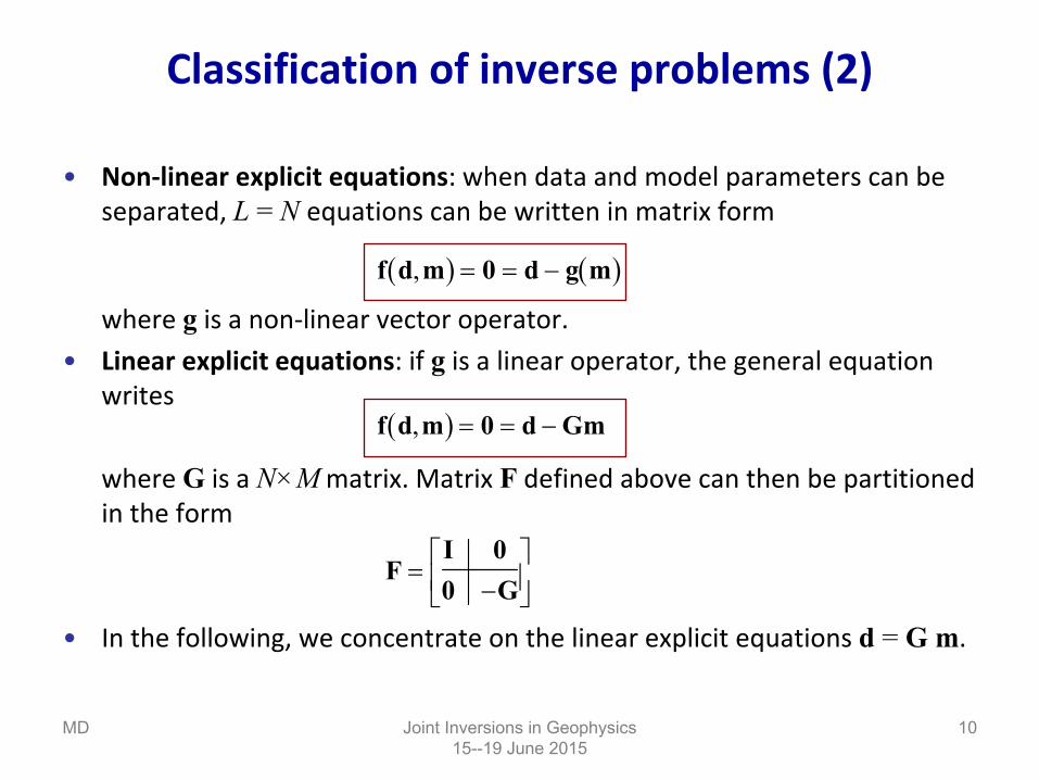
Non‐linear

explicit equations: when

data and

model

parameters

can

be separated, L

= N

equations

can

be

written

in matrix

form

where

g

is

a non‐linear vector operator.•

Linear

explicit equations: if g

is

a linear

operator, the

general

equation

writes

where

G is

a N×M

matrix. Matrix

F

defined

above

can

then

be

partitioned in the

form

•

In the

following, we

concentrate

on the

linear

explicit equations

d

= G m.


15--19 June

201510

Classification of

inverse problems

(2)

f d m 0 d g m,

f d m 0 d Gm,

FI 00 G

•

Simplest

mathematical

formulation. Uses linear

algebra

tools.•

Obey superposition and

scaling

laws:

G(m1

+ m2

) = Gm1

+ Gm2

G(αm) = α

Gm•

Broad

range of

applications: seemingly

non‐linear

problems

can

be

cast

in a

linear

form

(see

next

examples).•

Mathematical

linearity

is

associated

with

physical

linearity

(straight rays, …)

•

Can be

used

as local approximations for (weakly) non‐linear

problems


15--19 June

201511

Discrete

linear

systems

,2,1,0;)ˆ(

ˆˆ)ˆ()(

1

nnnn

nnn

mGmgmmmgmgmgd around expansion series Taylor

nnnj

iijnn m

gn

mmmGgG mm ˆ;ˆ

; 1)(ˆ

where

) from (starting for Invert 011)ˆ( mmmGmgdd nnnn

•

Problem of

fitting

a function

to a data set. The

function

is

defined

by a series

of

parameters.

•

When

the

problem

can

be

solved

as a linear

inverse problem, it

is

referred to a linear

regression.

•

Example: ballistic

trajectory


15--19 June

201512

Linear

regression

(Space Archive)

MNN z

zzz

mmm

tt

tttttt

tmtmmtz

3

2

1

3

2

1

2

233

222

211

2321

211

211211211

21)(Quadratic

in time

t, but linear

with

respect to mi

•

Deals with

path‐integrated

properties:–

Travel

times

of

acoustic, seismic, EM waves–

Attenuation

of

waves, of

X‐rays, of

muons–

…

•

In seismic

traveltime

tomography, the problem

is

non‐linear

if it

is

expressed

in

terms

of

wave

velocities

v.

•

It

is

linearized

by considering

the

wave slowness

u.

•

In case of

slowness

perturbations,

•

If the

medium is

discretized

into

blocks


15--19 June

201513

Tomography

ss

dssusv

dsT )()(

s

predobs dssuTTT )(

jj

iji ulT


15--19 June

201514

Tomographic reconstructionvia backprojection

Mo Dai Master 1 EGID U. Bordeaux 3

•

One

way

of

solving

the

linear

inverse problem

is

to measure

the

«

length

» of

some

vectors.

•

This is

related

to the

problem

of

minimizing

a misfit

function, which

will

be addressed

later

on in this

course.

•

For example, the

linear

regression

problem

issolved

by the

so‐called

least

squares method

in

which

one

tries to minimize

the

overall

error

•

The

least

squares method

uses the

L2

(or Euclidean) norm

which

is

defined, for a vector

v, by


15--19 June

201515

Vector

norms

(1)

). vectorof length Euclidean (squared

where

eee

Gmd

T

estpreprei

obsii

N

ii

E

ddeeE

;1

2

2/12/1

22 ),( vvv

i

iv

•

Other norms can be used such as

the

L1

norm

which

is

a particular

case of

the

Lp

norm

•

The

higher

norms

give

the

largestelement

of

vector

v

a larger

weight.

•

The

limiting

case p

→∞ is

the

L∞

norm

which

selects the

vector

element

with

the

largest

absolute

value as the measure

of

length.


15--19 June

201516

Vector

norms

(2)

v 1 ii

v

v i

ivmax

1/1

pvp

i

pipv

Outlier

•

Why

is

the

L2

norm

so

frequently

used? / Which

norm

should

we

use?1.

Computations are simpler

with

the

L2

norm

than

with

the

L1

norm.2.

Depends

on the

importance one

chooses

to give

to outliers, i.e., data that

fall

far from

the

mean

trend:–

If the

data are very

accurate

with

only

a few

outliers, we

may

want

to be

sensitive to these

anomalous

values. In this

case, we

would

use a high‐order norm.

–

On the

contrary, if the

data scatter

widely

around

the

trend, then

the

large prediction

errors

do not

carry a special

significance. In such

cases, a low‐order

norm

would

be

used

because it

gives

a more balanced

weight

to errors

of different

size.

3.

Similar

arguments could

be

developed

by considering

a probabilistic approach

of

the

inverse problem. Let us just

point out that

the

L2

norm implies

that

the

data obey

Gaussian

statistics. Gaussians

are rather

short‐

tailed

(limited

support) distributions which

imply

very

few

scattered

points.


15--19 June

201517

Vector

norms

(3)

•

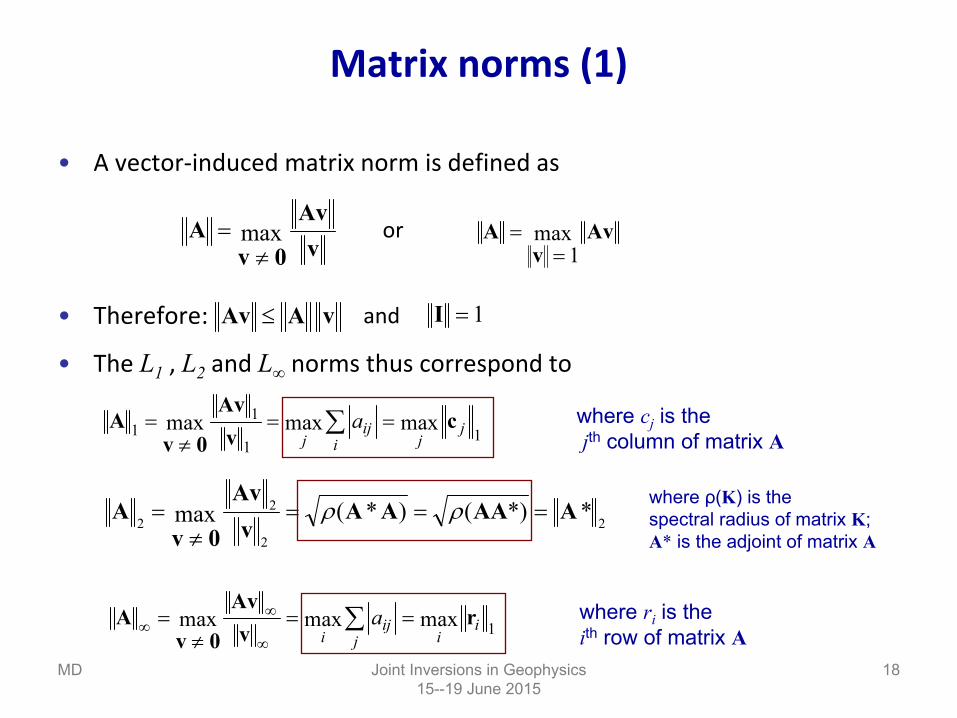
A vector‐induced

matrix

norm

is

defined

as

•

Therefore:

•

The

L1

, L2

and

L∞

norms thus correspond to


15--19 June

201518

Matrix

norms

(1)

orv

Av

0vA max

A

vAv

1max

andvAAv I 1

22

22

**)()*(max AAAAAv

Av

0vA

where

cj

is

thejth

column

of

matrix

AA

v 0

Avv

c11

11

max max maxj

iji j

ja

Av 0

Avv

r

max max maxi

ijj i

ia 1where

ri

is

theith

row

of

matrix

A

where ρ(K) is

thespectral radius of

matrix

K;A*

is

the

adjoint of

matrix

A

•

The

L1

norm

of

matrix

A

is

the

largest

L1

norm

of

the

columns

of

the

matrix.

•

The

L∞

norm

of

matrix

A

is

the

largest

L∞

norm

of

the

rows

of

the

matrix.

•

Both

are easily

calculated

from

the

elements

of

matrix

A.

•

The

L2

norm

of

matrix

A

requires

more computations. Let us give

a few practical

reminders

on matrix

calculation.

–

Transpose

–

Adjoint

–

Trace

–

Eigenvalue

/ eigenvector

problem

–

Characteristic

polynomial

–

Spectral radius

–

Singular

values


15--19 June

201519

Matrix

norms

(2)

( )*A ij jiajiij

T a)(A

N

iiia

1)tr(A

A x x

det( )A I N 0

.)(max)(1

AA iNi

i iT

iT( ) ( ) ( )A A A AA

For square matrices

•

The

L2

norm

of

matrix

A

is

the

largest

square root

of

the

eigenvalue

of matrix

AA*

or matrix

A*A.

•

It

is

the

largest

singular

value of

matrix

A.

•

If matrix

A

is

hermitian

(or self‐adjoint) A

= A*, or symmetric

A

= AT, its

L2

norm

is

the

spectral radius of

matrix

A:

•

The

Frobenius norm

is

not

vector‐induced

but can

easily

be

computed

•

It

is

an effective way

to compute

the

L2

norm

of

a matrix

since


15--19 June

201520

Matrix

norms

(3)

)(.)(2

AAAA norm, any For

or2/1

1 1

2

N

i

M

jijF

aA A A AF tr * /1 2

matrix. a for NNNF

22

AAA

•

Let’s consider

the

linear

system Au = b (taken

from

Ciarlet, 1994)

and

the

perturbed

system

•

A very

weak

relative perturbation of

the

RHSinduces

an important relative error

of

the

solution

that

is, an amplification of

the

relative errors

of

8.2 / 0.003 = 2461.Joint Inversions in Geophysics

15--19 June

201521

Conditioning

of

a linear

system

(1)

,

1111

31332332

1095791068565778710

4

3

2

1

is solution whose

uuuu

.

1.15.4

6.122.9

9.301.339.221.32

1095791068565778710

44

33

22

11

is solution whose

uuuuuuuu

0033.060/2.0/ bb2.82/4.16/ uu

MD

•

Let’s also

consider

a perturbed

system

in which

we

slightly

modify

the elements

of

matrix

A:

•

These

error

amplifications may

be

surprising

in this

example, considering

the good

aspect of

the

original matrix

A

which

is

symmetric

and

full, its

determinant

is

equal

to 1, and

its

inverse

Joint Inversions in Geophysics

15--19 June

201522

Conditioning

of

a linear

system

(2)

MD

.

97.2110.34

13633.80

31332332

98.9999.499.6989.998.585604.508.72.71.8710

44

33

22

11

is solution whose

uuuuuuuu

23106351710

101768416104125

1A doesn’t

show anything

special.

•

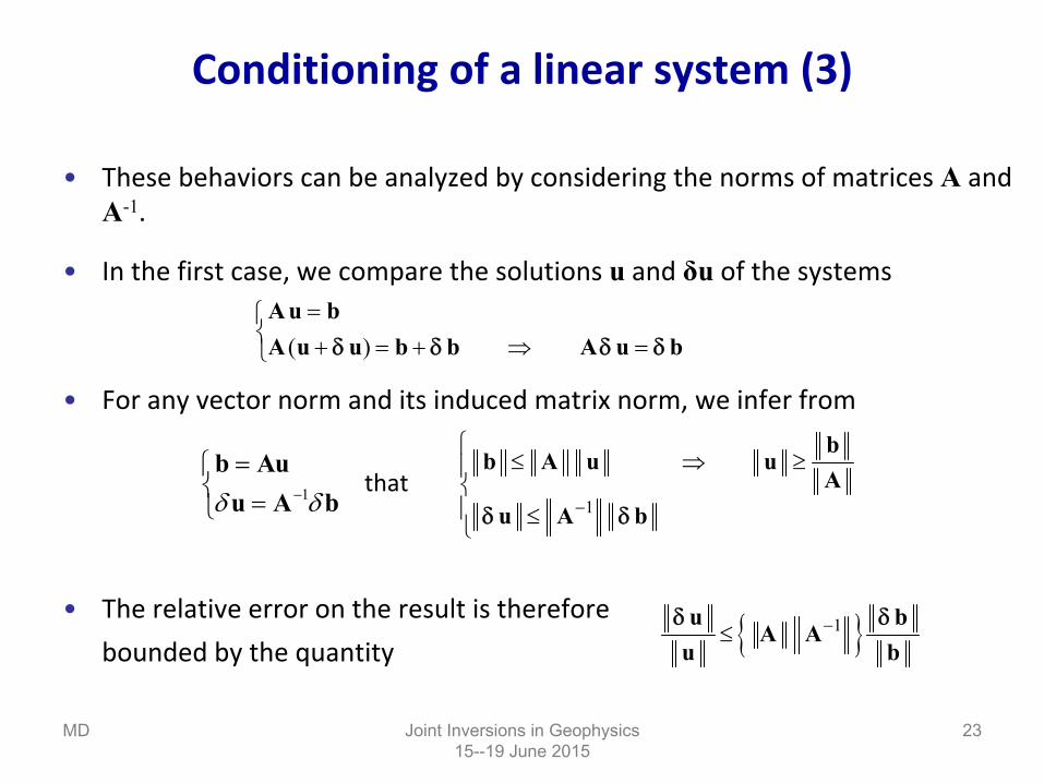
These

behaviors

can

be

analyzed

by considering

the

norms

of

matrices A

and A-1.

•

In the

first

case, we

compare the

solutions u

and

δu

of

the

systems

•

For any

vector

norm

and

its

induced

matrix

norm, we

infer

from

•

The

relative error

on the

result

is

thereforebounded

by the

quantity


15--19 June

201523

Conditioning

of

a linear

system

(3)

MD

A u bA u u b b A u b

( )

thatbAu

uAb 1

b A u ubA

u A b

1

uu

A Ab

b 1

•

In the second case, we compare the solutions u

and Δu

of

the

systems

•

We

infer

from

the

last

equality

that

•

For small

perturbations ΔA, is

a good

approximation of

and

therefore,

•

In both

cases, the

relative error

on the

result

is

bounded

by the

relative error

of

the

modified

quantities

multiplied

by

which

is

the

condition number

of

matrix

A. Joint Inversions in Geophysics

15--19 June

201524

Conditioning

of

a linear

system

(4)

MD

A u bA A u u b A u A u u

( )( ) ( )

is, thatuuAAu 1

uu u

A AA

A 1

u

u u uu

uu

A AA

A 1

cond( )A A A 1

•

The

condition number

measures

the

sensitivity

of

the

solution u

of

system Au =

b with

respect to variations in data b

or in elements

of

matrix

A.

•

A linear

system

is

well‐conditioned

if its

condition number

is

small; it

is

ill‐conditioned

if its

condition number

is

large.

•

Properties


15--19 June

201525

Conditioning

of

a linear

system

(5)

MD) ( matrix unitary a is if

) ( matrix normal a is if

matrixof zero‐non the denote where

matrixof zero‐non the denote where

) (since

IAAAAAAAAAAA

AseigenvalueA

A

AA

Avaluessingular A

A

AA

AAAA

AAIIAAA

**1)(cond**

)(

)(min

)(max)(cond

)()(min

)(max)(cond

)cond()cond()cond()cond(

1,1)cond(

2

2

2

1

11

i

ii

ii

i

i

i

i

i

•

Finally, cond2

(A)

is

invariant by unitary

transformation.

then

•

Numerical

analysis

of

the

previous

example

The

eigenvalues

of

symmetric

matrix

are equal

to its

singular

values

Using

L2

norm,

so

that

condition becomes

8.199 < 9.942 .


15--19 June

201526

Conditioning

of

a linear

system

(6)

MD

UU U U I* *

.)(cond)(cond)(cond)(cond *2222 AUUAUUAA

A

10 7 8 77 5 6 58 6 10 97 5 9 10

01015.08431.0858.32887.30 4321

025.602.0;

2397.16;108.2984)(cond

2

2

2

2

4

12

bbδ

uuδ

A

uu

Ab

b2

22

2

2 cond ( )

•

The

Frobenius norm

is

useful

to evaluate

the

L2

norm

of

a matrix

without knowing

its

singular

values.

•

Here, for symmetric

matrix

A,

•

Therefore,

which

verifies

property

seen

previously

•

We

also

verify

that

leading

to 0,998 < 26,267 .


15--19 June

201527

Conditioning

of

a linear

system

(7)

MD

F

F

1

4

1

2

1

12

5292.985222.981)(

5450.302887.30)(

AAA

AAA

cond cond2 21

212984 3009( ) ( )A A A A A A

F F F

22AAA N

F

uu u

AA

A cond( )

uu u

AA

F

F

F

F

162 825163 079

030 5450

,,

; ,266645,

•

When

solving

the

linear

inverse problem

d =

Gm, several

cases must be distinguished

according

to the

quantity

of

information contained

in the

equation

d =

Gm.

•

This information depends

on number

N

of

data and

number

M of

model parameters, but it

also

depends

on the

structure of

matrix

G which

can

be

sparse

or full.

•

If N > M, there

are more data than

unknowns, i.e., too much information to exactly

solve

the

inverse problem.

This corresponds to an overdetermined

problem.Curve

(or surface) fitting

procedures

are typical

overdetermined

problems.

•

If N < M, there

are more unknowns

than

data:we

do not

have enough information to determine

all

model

parameters.

This corresponds to an underdetermined

problem.


15--19 June

201528

Classification of

linear

inverse problems

(1)

MD

•

In reality, we

often

must deal with

mixed‐determined

problems, which

are partly

overdetermined

and

partly

undertermined.

This can happen even if N > M.

•

This situation is

typical

of

tomographic

experiments

when

the

medium is divided

into

blocks: some

blocks are crossed

by many

rays whereas

others

are not

crossed

by any

rays.

•

Each

of

the

situations described

abovemust be

solved

in an appropriate

manner.

•

The

solution for mixed‐determinedproblems

applies

to all

situations

but is

not

necessarily

optimal.


15--19 June

201529

Classification of

linear

inverse problems

(2)

MD

•

Minimization

of

the

prediction

error

in overdetermined

problems.

•

Minimization

of

the

norm

of

the

estimated

solution in underdetermined problems.

•

Combination

of

the

two

approaches

in mixed‐determined

problems.


15--19 June

201530

Solutions based

on norm

minimization

MD

•

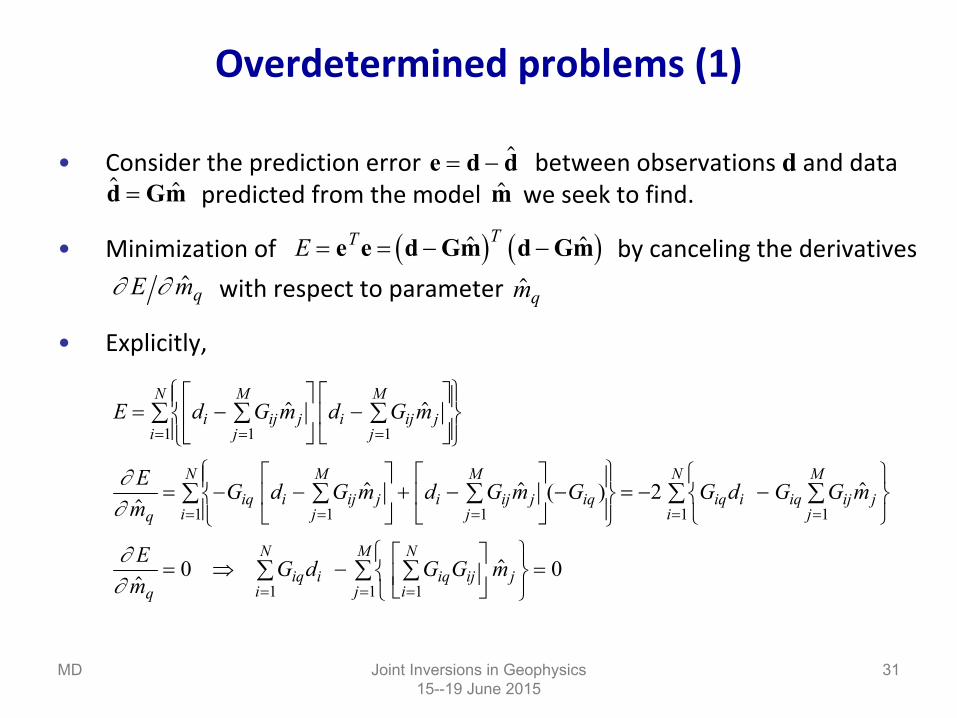
Consider

the

prediction

error

between

observations d

and

data predicted

from

the

model

we

seek

to find.

•

Minimization

of

by canceling

the

derivativeswith

respect to parameter

•

Explicitly,


15--19 June

201531

Overdetermined

problems

(1)

MD

e d d d Gm m

E T T e e d Gm d Gm

E mq mq

E d G m d G m

Em

G d G m d G m G G d G G m

Em

G d G G

i ij jj

Mi ij j

j

M

i

N

qiq i ij j

j

Mi ij j

j

Miq

i

Niq i iq ij j

j

M

i

N

qiq i iq ij

i

N

( )

1 11

1 11 11

1

2

0

mjj

M

i

N

110

•

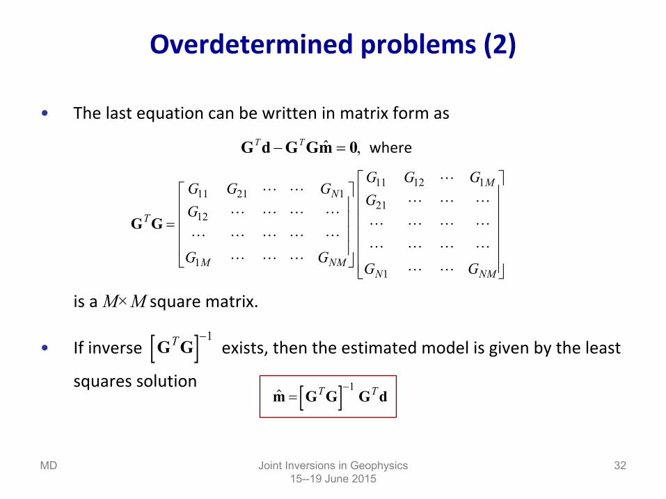
The

last

equation

can

be

written

in matrix

form

as

is

a M×M square matrix.

•

If inverse exists, then

the

estimated

model

is

given

by the

least squares solution


15--19 June

201532

Overdetermined

problems

(2)

MD

where,ˆ 0mGGdG TT

G GT

N

M NM

M

N NM

G G GG

G G

G G GG

G G

11 21 1

12

1

11 12 1

21

1

G GT 1

m G G G dT T1


15--19 June

201533

311282

211M

3 × 3 model

Tomographic reconstruction of a 3 × 3 model (1)

16-ray scan of the model

-1 1 2

2 8 -2

1 -1 3-13

11-3

3 11

10

-12

2

8

3

2 8 3Note: it

is

assumed

that

allray segmentshave unit length


15--19 June

201534

corner) right lower to corner left upper (from

corner) left ower l to corner right upper (from

) right to left from (

) bottom to top from (

SW" ‐ NE" rays oblique 5

SE"‐NW" rays oblique 5

rays vertical 3

rays horizontal 3

100000000010100000001010100000001010000000001001000000010001000100010001000100010000000100100100100010010010001001001111000000000111000000000111

G

311282211

m

1 2 3

4 5 6

7 8 9

Cell numbering adopted

Matrix of raypaths(other expressions are also possible)


Data vector

d


15--19 June

201535

311282

211M

1991773714

181213M̂

311282

211~M

True model Back-projection Filtered back-projection

m dGm Tˆ mGGdGGGm ˆ~ 11 TTT

(Maple

computations and

graphics)


•

When

the

number

of

unknowns, M, exceeds

the

number

of

data, N, the problem

admits

an infinity

of

solutions.

•

To obtain

a solution, one

has

to provide

some

a priori information (e.g., physical

constraints) to reduce

the

number

of

solutions.

•

We

can

also

find

a solution minimizing

the

norm

of

the

model

while imposing

at the same time a zero

prediction

error.

•

This problem

can

be

solved

with

Lagrange multipliers

which

we

first illustrate

with

the

minimization

of

a function

of

two

variables E(x,y)

subject

to a constraint

φ(x,y) = 0

defined

implicitly.

•

Minimize

λ: Lagrange multiplier


15--19 June

201536

Underdetermined

problems

(1)

MD

L mTj

j

M

m m

e d Gm 0

2

1Minimum

= - =

dE d Ex x

dx Ey y

dy

0

•

Since

dx

and

dy

are not

independent, we

have to consider

the

3 equations

that will allow us to determine the 3 unknowns: the values of x

and y

at the minimum of function E, and λ

(not

needed).

•

When

we

have M unknowns

in a vector

and

N

constraints

, we introduce

a Lagrange multiplier for each

constraint.

We

then

have to solve

M+N

simultaneous

equations

for M+N

unknowns.

•

In our

underdetermined

problem, we

minimize

the

function


15--19 June

201537

Underdetermined

problems

(2)

MD

Ex x

Ey y

x y

0 0 0; ; ( , )

m ( )m

variables to respect with

MqmmGdmeL

q

N

i

M

jjijii

M

jji

N

ii ,1,ˆ

ˆˆ)ˆ(1 11

2

1

m

•

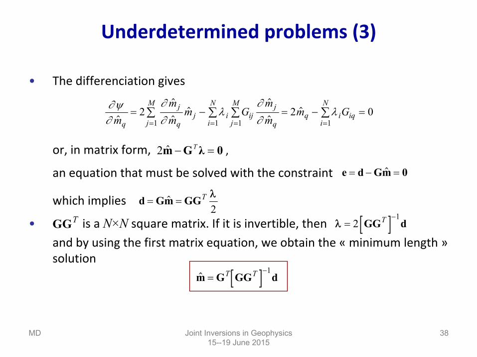
The

differenciation

gives

or, in matrix

form,

an equation

that

must be

solved

with

the

constraint

which

implies

• is

a N×N

square matrix. If it

is

invertible, then

and

by using

the

first

matrix

equation, we

obtain

the

«

minimum length

» solution


15--19 June

201538

Underdetermined

problems

(3)

MD

mmm

m Gmm

m Gq

j

qj

Mj i

i

Nij

j

M j

qq i

i

Niq

2 2 0

1 1 1 1

,0λGm Tˆ2

e d Gm 0

d Gm GG T 2

GGT

21

GG dT

m G GG dT T 1

(a) (b) (c)

overdetermined

underdetermined

2 parameters, 3 data > 1 information

•

Example

taken

from

Menke

(1984).

•

We

can

only

determine

the

average

properties

of

the

two

cells

in case c).


15--19 June

201539

Mixed‐determined

problems

(1)

MD

G m G m dG m G m dG m G m d

11 1 12 2 1

21 1 22 2 2

31 1 32 2 3

212

211

212

211

2

2mmmmmm

mmm

mmmthen gintroducin By

323122211211

313231

212221

111211

;; GGGGGGdmGGdmGGdmGG

since

•

This shows that

parameter

m’1

is

overdetermined

whereas

parameter

m’2

is

underdetermined. This suggests

a partitioning

of

the

equations

into

overdetermined

and

underdetermined

parts by forming

linear combinations

of

the

initial parameters.

•

The

new problem

d'=G'm'

can

be

solved

by using

the

least

squares solution for the

overdetermined

part and

the

minimum length

solution

for the

underdetermined

part, i.e., we

minimize

the

data prediction

error and

introduce

only

minimal a priori information.

•

For this, we

write

equation

d

= Gm

in the

form

, where belong

to the

model

nul space

and

data nul space,

respectively:


15--19 June

201540

Mixed‐determined

problems

(2)

MD

under

over

under

over

under

over

dd

mm

G00G

00 dm and d d G m mr r 0 0

.000 Gmd0Gm Tand

•

With

this

decomposition, prediction

error

E

and

norm

of

solution L

write:

•

Returning

to the fact that we want to minimize

the

data prediction

error and

introduce

only

minimal a priori information, we

therefore

impose

and

we

may

choose to limit

a priori information.

•

The

vector

subspaces

belong

to can be identified by a

SVD of

matrix

G which

writes

•

are matrices of

dimensions N×r, r×r, and

M×r, respectively.


15--19 June

201541

Mixed‐determined

problems

(3)

MD

0

0

0000

00000

rTT

rT

rTr

T

Trr

TTrr

Trr

T

L

E

mmmmmmmmmm

dddd0GmddGmdGmd

GmdGmd

since

andas

Er r rT

r r d Gm d Gm 0

m 00

(Error

on d0

cannot

be

reduced)

00 ,, ddmm andrr

G U V r r rT

rrr VU and,

•

is

a diagonal matrix

containing

the

r

non‐zero

singular

values of

matrix

G.

•

Ur

contains

the

eigenvectors

associated

with

the

non‐zero

eigenvalues

of matrix

GGT.

•

Vr

contains

the

eigenvectors

associated

with

the

non‐zero

eigenvalues

of matrix

GTG.

•

We

introduce

U0

and

V0

as the

contributions of

zero

singular

values of

G.

•

With

these

definitions, mr

, m0

, dr

and

d0

belong

to the

subspaces

spanned by Vr

, V0

, Ur

and

U0

.

•

Notes on the

nul spaces

U0 and

V0

:–

It

is

easy

to verify

thatThis implies

that

the

data cannot

entirely

be

described

by operator

G

–

V0

is

responsible

for the

non‐uniqueness

of

the

solutions because


15--19 June

201542

Mixed‐determined

problems

(4)

MD

r

.000 rTrrr

TT UU0mVUUGmU because

0GmGmmmGVm 0since1010 )(,0

•

By analogy

with

square matrices G, for which

the

inverse operator

is

G-1, since we have , we

define

for our

mixed‐determined

problem

d

= Gm

a «

generalized

»

inverse so

that

•

We

can

easily

verify

that

this

solution–

Has

no

component in the

model

nul space

V0

:

–

Error

e

has

no

components in Ur

subspace


15--19 June

201543

Mixed‐determined

problems

(5)

MD

G U V r r rT

G V U gr r r

T 1

dUVdGm Trrr

g 1ˆ

rTrrr

TT VVdUVVmV 0

100 0ˆ as

rrTrrr

Tr IVVIUU andSince

0dUdUdUUdU

dUVVUdU

mGdUeU

Tr

Tr

Trr

Tr

Trrr

Trrr

Tr

Tr

Tr

1

ˆ

•

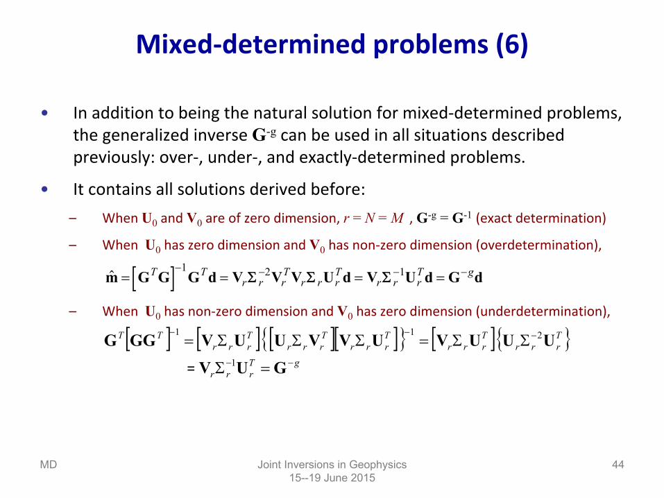
In addition to being

the

natural

solution for mixed‐determined

problems, the

generalized

inverse G-g

can

be

used

in all

situations described previously: over‐, under‐, and

exactly‐determined

problems.

•

It

contains

all

solutions derived

before:–

When

U0

and

V0

are of

zero

dimension, r = N = M

, G-g

= G-1

(exact determination)

–

When

U0

has

zero

dimension and

V0

has

non‐zero

dimension (overdetermination),

–

When

U0

has

non‐zero

dimension and

V0

has

zero

dimension (underdetermination),


15--19 June

201544

Mixed‐determined

problems

(6)

MD

m G G G d V V V U d V U d G d T T

r r rT

r r rT

r r rT g1 2 1

gT

rrr

Trrr

Trrr

Trrr

Trrr

Trrr

TT

GUV

UUUVUVVUUVGGG1

211

=

•

In case of

weak

underdetermination, rather

than

partitioning

vectors

m and

d, we

can

minimize

a combination

of

the

data prediction

error

E

and

length

of

the

solution L, i.e., we

minimize

a function

with

respect to elements

of

model

we

seek

to find.

•

Factor

ε

determines

the

importance of

length

L

relative to error

E

in the minimization

of

function

.

•

By solving

this

minimization

problem explicitly, we end up with the damped

least

squares solution

•

The

additional

term

ε2I

regularizes

matrix

GTG

and

stabilizes

its

inverse, at the

expense

of

the

model

resolution.


15--19 June

201545

Weak

underdetermination

MD

( ) m e e m m E L T T2 2

mq m

( )m

m G G I G d T T 2 1

•

The

criterion

that

was

adopted

(minimization

of ) is

not

always

suitable. It

can

be

generalized

in several

ways.

•

For instance, we

can

introduce

an a priori information on the

model

and consider

minimizing

•

In other

cases, we

will

be

looking

for smooth

solutions by introducing weighting

factors

in the

form

of

a M×M matrix

Wm

:

•

We

may

estimate

the

roughness

of

discrete

model

parameters

via


15--19 June

201546

Other

a priori information (1)

MD

mmTL

prioriT

prioriL mmmm

.mWm mTL

Mm

mm

2

1

11

1111

Dm

•

Matrix

D

is

an approximate

differenciation

operator. Minimizing

the roughness

of

vector

m

amounts

to minimize

•

The

off‐diagonal

terms

of

matrix

Wm

represent

the

interdependence

of the

model

parameters. Matrix

Wm

can be designed to impose some relationship

between

the

model

parameters.

•

By combining

the

a priori information mpriori

and

weighting

matrix

Wm

,

•

We

can

similarly

define

a N×N

weighting

matrix

Wd

for the

data to favor the

«

good

»

data at the expense of the noisy data and

define

a

generalized

prediction

error

Wd

is

a diagonal matrix

when

there

is

no

coupling

between

the

data.Joint Inversions in Geophysics

15--19 June

201547

Other


MD

mWmmDDmDmDm mTTTTTL

priorimT

prioriL mmWmm

eWe dTE

•

We

thus

obtain

new solutions of

the

discrete

linear

inverse problem, which

generalize

the

expressions obtained

so

far.

•

Overdetermined

problems

Minimization

of

leads

to the

weighted

least

squares solution

•

Purely

underdetermined

problems

Minimization

of

with

constaint

E = 0

leads

to the

weighted

minimal length

solution


15--19 June

201548

Other


MD

eWe dTE

dWGGWGm dT

dT 1

ˆ

priorimT

prioriL mmWmm

prioriT

mT

mpriori GmdGGWGWmm 1

ˆ

•

Weakly

underdetermined

problems

Minimization

of

quantity

leads

to the

damped

and

weighted

least

squares solution which

can

be written

•

Linear

equality

constraints: yet another class of

a priori information Linear

combinations

of

model

parameters

can

be

expressed

as h

= Fm.

For example, if the

average

of

the

model

parameters

is

equal

to a constant µ, then


15--19 June

201549

Other


MD

priorimT

prioridTLE mmWmmeWem ˆˆ)ˆ( 22

priorid

Tm

Tmpriori

prioridT

mdT

priori

GmdWGGWGWmm

GmdWGWGWGmm

11211

12

ˆ

ˆ

hFm

Mm

mm

M 2

1

11111

•

Other

example: in a curve

fitting

procedure, impose that

the

curve

passes through

a specified

point.

•

One

way

to account

for linear

equality

constraints

is

to combine the

p equations

h

= Fm

with

the

N

equations

d

= Gm

and

to put strong

weights

on equations

h

= Fm.

•

This will

impose a prediction

errorwhich

is

very

small

for the

equations

h

= Fm

at the

expense

of

theprediction

error

of

equations

d

= Gm

which

can

be

important.


15--19 June

201550

Other


MD

•

Another

solution to this

problem

is

to minimize

the

prediction

error E

= eTe

with

the

p

constraints

Fm

–

h

= 0

by using

the

Lagrange multipliers

technique once more.

•

We

minimize

the

function

•

In matrix

form:

•

Finally, the

solution of

the

overdetermined

problem

d

= Gm

with

linear constraints

h

= Fm

is


15--19 June

201551

Other


MD

MqmhmFdmG q

p

i

M

jijiji

N

i

M

jijij ,1,ˆˆ2ˆ)ˆ(

1 11

2

1

variables wrt m

hdGm

0FFGG TTT

ˆ

hdGGGFFGGFFGGdGGGm TTTTTTTT 11111ˆ

constraintwithoutsol.

•

We

have obtained

model

parameters

estimates

in various

situations that we

can

write

•

The

inverse operator

G-g

is

not

a matrix

inverse in the

classical

sense (except

in the

exactly

determined

problem where

G-g

= G-1). The

matrix products

GG-g

and

G-g

G

are generally

not

identity

matrices.

•

Data predicted

from

the

estimated

models

are obtained

via

•

The

N×N

square matrix

is

the

data resolution

matrix, which should

ideally

be

the

IN

identity

matrix. In this

case, the

data prediction error

would

be

zero.

•

The

importance of

off‐diagonal

terms

can

be

evaluated

by defining


15--19 June

201552

Properties

of

generalized

inverses (1)

MD

vdGm obsgest

obsobsgobsgestpre dNdGGdGGGmd

g GGN

2

1 1

2)(

N

i

N

jijijFN n IΝN

•

Similarly, we

may

wonder

how

close the

estimated

model

mest

is

from

the true

model

mtrue

which is such that Gmtrue

= dobs.

•

Therefore,

•

The

M×M square matrix

is

the

model

resolution

matrix, which should

ideally

be

the

IM

identity

matrix

to uniquely

determine

each

model parameter.

•

The

importance of

off‐diagonal

terms

can

be

evaluated

by defining

•

The

unit covariance matrix

characterizes

the

degree

of

error

amplification that

occurs

in the

mapping

from

data to model

parameters. If the

data are

all

uncorrelated

and

have equal

variance σ2, the

unit covariance matrix

is given

by


15--19 June

201553

Properties

of

generalized

inverses (2)

MD

truetruegtruegobsgest mRmGGGmGdGm

GGR g

2

1 1

2)(

M

i

M

jijijFM r IRR

TggTgd

g GGGCGΓ 2

•

If N

> M: Overdetermined

problem–

Minimization

of

prediction

error

–

Least

squares solution

–

Data resolution

matrix

–

Model resolution

matrix

–

Unit covariance matrix

•

If N

< M: Underdetermined

problem–

Minimization

of

norm

of

solution with

constraint

E

= 0

–

Minimum length

solution

–

Data resolution

matrix

–

Model resolution

matrix

–



15--19 June

201554

Summary

(1)

MD

Resolution

of

linear

systems

d

= Gm

for N

data and

M

unknowns

using

the

L2

norm

E T d Gm d Gm

dGGGm TT 1ˆ

N G G G GT T1

MIR

G GT 1

L T m m

dGGGm 1ˆ TT

N I N

GGGGR 1 TT

G GG GT T 2

•

For any

given

N, M: Mixed‐determined

problem–

Singular

value decompostion

–

Generalized

inverse solution

–

Data resolution

matrix

–

Model resolution

matrix

–


•

Damped

least

squares solutions


15--19 June

201555

Summary

(2)

MD

Resolution

of

linear

systems

d

= Gm

for N

data and

M

unknowns

using

the

L2

norm

G U V r r rT

m V U d r r rT

N U U r rT

TrrVVR

V Vr r rT2

m G G I G d T

MT 2 1

m G GG I d T T

N 2 1

Exercise: medium described by 4 cells

•

Compute solutions with

•

In all these cases, computethe solution length the data prediction error

dGGGm TT 11ˆ

1,1.0,01.0;ˆ 123

dIGGGm NTT

1,1.0,01.0;ˆ 123

dGIGGm TM

T

dUVm Trrr4ˆ

E T T e e d Gm d Gm

mm ˆˆ TL


•

Use your preferred computation tool to do the matrix operations:

–

Matlab, Octave

–

Maple, Mathematica

–

LibreOffice, Gnumeric, Excel (MMULT, MINVERSE, TRANSPOSE, …)(*)

–

Python, R

–

Fortran, C

(*) Norms can be tricky to compute


•

Main results: 109;0;8542ˆ 111 LEm

0.1][0108.513814;2-8e.242736090

97.9759273434.9908527273.9958278452.00577809ˆ

33

3

LEm

0.01][1108.996320;6-0e.147900000

7.9997904.9999403.9999902.000090ˆ

22

2

LEm

0.1][1108.513802;2-3e.242747831

7.975927054.990852413.995827532.00577777ˆ

22

2

LEm


•

Main results (continued):

Solid line: damped overdetermined

solutionSymbols: damped underdetermined solution


•

Main results (continued):6×6 data resolution matrix

for

the least squares solution (1)

Data predicted from theestimated model do notentirely explain the data(they are slightly smoothed)

4×4 model resolution matrix

forthe least squares solution isI4

identity matrix


•

Main results (continued):When ε

increases

(> 0.6),

we

degrade

both

thedata and

model

resolutions

(smoothing)

Trade‐off

betweenresolution

and

variance

µ(R)

µ(N)tr(Γ)

tr(N,M)

training course on joint inversions in...

Documents