1  

Transaction Costs, Communication and Spatial Coordination in Payment for Ecosystem Services Schemes∗

Simanti Banerjee

University of Nebraska-Lincoln Email: simanti.banerjee@unl.edu

Timothy N. Cason Purdue University

Email: cason@purdue.edu

Frans P. de Vries University of Stirling

Email: f.p.devries@stir.ac.uk

Nick Hanley University of St. Andrews

Email: ndh3@st-andrews.ac.uk

30 August 2016

Abstract

Landowner participation and spatial coordination of land use decisions are key components for enhancing the effective delivery of ecosystem services from private land. However, inducing landowner participation in Payment for Ecosystem Services schemes for coordinating land management choices is challenging from a policy design perspective owing to transaction costs associated with participation. This paper employs a laboratory experiment to investigate the impact of such costs on participation and land use in the context of an Agglomeration Bonus (AB) scheme. The AB creates a coordination game with multiple Nash equilibria relating to alternative spatially-coordinated land use patterns. The experiment varies transaction costs between two levels (high and low), which affects the risks and payoffs of coordinating on the different equilibria. Additionally, an option of costly communication is implemented between neighboring landowners arranged on a local network to facilitate spatial coordination. Results indicate a significant difference in participation and performance under high and low transaction costs, with lower uptake and performance when transaction costs are high. These effects are, however, impacted by transaction costs faced in the past. Communication improves both AB participation rates and performance with the effect being greater for participants facing high transaction costs.

                                                                                                                         ∗ We thank the European Investment Bank (EIB) for financial support under the EIB-University Research Action Programme (theme Financial and Economic Valuation of Environmental Impacts). The findings, interpretations and conclusions presented are entirely those of the authors and should not be attributed in any manner to the EIB. Any errors remain those of the authors. For helpful comments we thank Hernan Bejarano, Daniel Hellerstein, Gregory Parkhurst, Andrew Reeson and two anonymous referees; seminar participants at the University of Aberdeen, Indiana University, University of Michigan, Technical University Munich, Murdoch University, University of Montpellier, and audiences at the Annual BIOECON and Economic Science Association conferences. We also thank Ashlee Carlson, Mike Castle and John Bohaty for valuable research support.

2  

1. Introduction

Payment for Ecosystem Services (PES) or agri-environmental schemes offer landowners

financial incentives for actions designed to increase the supply of ecosystem services from

privately owned land (Hanley et al. 2012; Hanley and White 2014). In many instances, spatial

coordination is a desirable feature of such schemes, enabling the delivery of greater ecosystem

service benefits compared to a situation where the uptake of contracts is spatially uncoordinated.

Examples include greater biodiversity conservation benefits on farmland (Merckx et al. 2009;

Dallimer et al. 2010; Wätzold et al. 2010), successful species reintroduction programmes and

meta-population management on private land where habitat corridors permit wildlife

movements, or where certain minimum sized contiguous habitat is needed (Williams et al. 2005;

Önal and Briers 2006), enhanced water quality improvements (Lane et al. 2004; Lane et al.

2006), and native vegetation restoration (Windle et al. 2009).

Since participation in PES schemes is voluntary, economists have looked for means of

incentivising spatial coordination. One such mechanism is the Agglomeration Bonus (AB),

originally developed by Parkhurst et al. (2002). The AB is a two-part payment mechanism where

landowners receive compensation for participating/enrolling, plus a bonus if neighboring

landowners participate and select the same land use activity. In this format, the AB resembles a

coordination game with multiple Nash equilibria pertaining to different land use choices. The

Nash equilibria can be Pareto ranked by their payoffs. Laboratory experiments have indicated

that such a payment structure can produce a range of desired spatial patterns of enrolled land

parcels (Parkhurst and Shogren 2007; Warziniack et al. 2007). However, Banerjee et al. (2012;

2014) found that spatial coordination is challenging, and the AB can often fail to produce the

desired spatial patterns owing to coordination failure.

3  

Additionally, participation in any PES scheme is associated with landowner transaction

costs (Shortle et al. 1998; Kampas and White 2004). Examples of such costs include landowners’

travel time to meetings with government officials, the time and cognitive effort of determining

the relative payoffs of signing or not signing a contract, and the costs of engaging farm advisors.

Such transaction costs have been shown empirically to reduce participation in PES schemes

(Falconer and Saunders 2002; McCann et al. 2005; Mettepenningen et al. 2009). The AB, with

its more complex design, is likely to create additional transaction costs such as those associated

with negotiating with neighbors. It seems likely then that the success of the AB will be

influenced by the size of transaction costs relative to the payoffs of enrolling. Yet no analysis to

date has studied the effects of variations in transactions costs on the performance of the AB.

Fooks et al. (2016) is perhaps closest to our study, in which the transaction costs are implicitly

captured by a fixed submission fee. However, they studied a conservation auction and not a

subsidy scheme as considered here.

Our paper poses two main research questions. First, what is the degree of participation

and spatial coordination realized in AB schemes under different levels of transaction costs?

Second, to what extent can communication between neighboring landowners improve AB

performance by mitigating any negative effects of transaction costs? We answer these questions

using a laboratory experiment. Lab experiments are useful to this study because they bypass the

fact that it is not practical, and often even impossible, to exogenously manipulate the size of

transaction costs for PES schemes participation in the field; and because only a few PES

schemes in practice today include payments for spatial coordination (Kuhfuss et al. 2016). By

implementing a predefined fixed network structure in the laboratory, thus keeping the

4  

environmental complexity constant, the experiment allows us to specifically investigate how

varying transaction costs impact spatial coordination within an AB setting.

Our experiment is comprised of groups of subjects who decide whether to participate in

an AB scheme by paying a fixed fee – the transaction cost of participation. The transaction cost

treatment is manipulated in a within-subject design. Since we are interested in strategic

interactions and spatial coordination, we use a circular local network. On this type of network

every individual is connected to two neighbors (to their left and to their right) directly and

indirectly to the others in the network (Jackson 2010). While serving as a suitable framework

reflecting the decision problems of land managers on real landscapes, this specific network

structure also allows us to contribute to the experimental literature on equilibrium selection and

individual behavior in network coordination games (Berninghaus et al. 2002; Cassar 2007). The

network is also useful for implementing our between-subject communication treatment in a

format representative of social interactions in agricultural communities where communication

incurs a transaction cost and but is expected to be more frequent between geographical neighbors

than with others within a community.1

Our results indicate that participation is significantly higher when transactions costs are

low than when they are high. Moreover, in the event that individuals incur the transaction costs

and participate, we observe higher rates of spatial coordination. The role of communication is

not straightforward. Messaging unambiguously improves performance relative to no-

communication situations when transaction costs are high. However, its efficacy in low

                                                                                                                         1 In the field, transaction costs and costs of communication might vary with the degree of environmental complexity owing to individual and landscape heterogeneity (e.g., due to the amount and nature of land holdings, the number of landowners, or the extent of their social capital). However, the dynamics of these factors can make it difficult to isolate how transaction costs and communication affect spatial coordination. Thus, in this study, we have controlled the transaction cost and communication cost to be the same for every individual.

5  

transaction cost regimes depends upon whether subjects faced high costs in the past and had

previous experience with participating in the AB scheme.

2. The Strategic Environment

There are 𝑖 = 1,… ,𝑁 landowners who face two simultaneous decision opportunities. The

first decision entails whether or not to participate in the AB scheme. If a landowner decides to

participate, he or she can use his or her land for two different types of conservation land uses,

𝜎! = 𝑋,𝑌, which produce different levels and types of ecosystem services benefits. Our choice

decision is thus at the extensive margin and different from the original setup proposed in

Parkhurst and colleagues 2002; 2007 where subjects make an intensive margin choice of how

many acres to enroll. We have made this distinction so that our results may prove insightful in

understanding choices facing actual landowners where enrollment options in a PES scheme are

“all or nothing”, such as in the Conservation Stewardship Program under which the entire

eligible acreage has to be enrolled in specific land uses to receive payments (NRCS 2016).

We assume that the ecosystem service benefits delivered from coordination of land use

type X have greater agglomeration rewards than for type Y, and the regulator sets the AB

payments to reflect this ranking. Such differences in environmental benefits from spatial

coordination of enrollment might reflect differences in the ecological objectives of a scheme, or

in the kinds of land use change that are rewarded. Let 𝜎! =  NP denote non-participation for

landowner i whereby land is devoted to profit-based conventional agriculture, earning only

agricultural returns.2

                                                                                                                         2 Traditional agricultural land use practices (denoted by NP) can also deliver ecosystem services such as reduction in soil erosion and biodiversity benefits by providing nesting and foraging habitats. These benefits are, however, not additional as they are associated with business-as-usual land use practices. Since one of the criteria for receiving

6  

The AB scheme consists of two payoff components. The base component is a

participation subsidy, 𝑠 𝜎! , intended to compensate for any opportunity cost of conservation

relative to profit-maximising agricultural land use. Landowner i receives an additional

bonus,  𝑏 𝜎! , if a neighboring landowner implements the same conservation land use practice as

landowner i. Thus, the total bonus received is proportional to the number of neighboring

landowners choosing the same land use strategy, denoted by 𝑛!". We assume that the

environmental agency provides AB payments for adoption of pro-conservation land use of one

type only, i.e., landowners cannot choose both X and Y. We make this assumption because (i)

PES schemes typically involve a menu of land use practices from which landowners usually can

select a few suitable ones, and (ii) paying some landowners for undertaking all listed actions may

exhaust the limited PES budget (Cooper, Hart, and Baldock 2009; Armsworth et al. 2012),

creating high participation clusters in some areas at the expense of low participation rates

elsewhere.3 Let 𝑟 𝜎! denote the agricultural revenue under land use 𝜎! = 𝑋,𝑌,𝑁𝑃.

If a landowner i chooses to participate in the scheme he or she incurs transaction costs, 𝑇!.

We assume that all landowners have identical transaction costs, i.e., 𝑇! = 𝑇, either High or Low

depending on the treatment. In practice, these transaction costs will vary substantially across

landowners and across land use strategies. However, by sacrificing some realism (which would

probably not cause large behavioral differences) we gain tractability to identify causal treatment

effects. The payoff, 𝑢! 𝜎! , of landowner 𝑖 under the AB scheme reads as follows:

𝑢! 𝜎! =      𝑟 𝜎! + 𝑠 𝜎! + 𝑛!"𝑏 𝜎! − 𝑇          𝑖𝑓  𝜎! = 𝑋,𝑌      𝑟(𝜎!)                                                                                                    𝑖𝑓  𝜎! =  𝑁𝑃 (1)

                                                                                                                                                                                                                                                                                                                                                                                                       ecosystem services payments is additionality (Wunder 2007; Engel et al. 2008), such benefits should not be rewarded by the conservation agency. We therefore do not consider them in our model. 3 Such localized clustering may be interpreted as geographical targeting of conservation funds which can be politically contentious to the extent that the U.S. Congress has prohibited such targeting (Shortle et al., 2012).

7  

In Eq. (1) the number of neighbors and hence the bonus payment is contingent on the

specific landscape structure. Following Banerjee et al. (2012, 2014), in this study we impose a

simple circular network structure to represent neighborhood interactions. On such a circular local

network 𝑛!" can either take the value 0, 1 or 2. By employing a circular network each individual

faces the same level of strategic uncertainty within the decision environment, since all have the

same number of neighbors. Given this spatial symmetry in terms of the individuals’ location on

the network, we avoid additional complications, such as holdout problems due to bargaining

power of some individuals that are strategically located. In networks featuring an asymmetric

neighborhood structure (e.g., a two-dimensional lattice grid or a straight-line), individuals could

respond differently to the transaction cost variation and information available through

communication.

We note here that while the choice of network structure is simpler than the more complex

spatial grids implemented by Parkhurst et al. (2002) and Parkhurst and Shogren (2007) to study

spatial targeting, it still captures the main strategic interdependencies that are relevant for

studying spatially contiguous land use. First, in many realistic environments, individuals

typically do not interact with all individuals within their network directly but perhaps only

interact with a few neighboring individuals who provide them with information about what

others within the same network are doing. Second, like more complex spatial grids, a circular

network also exhibits strategic uncertainty regarding individuals’ decision-making, especially if

individuals have imperfect information about the choices of individuals that are not their direct

neighbors (see Banerjee et al., 2014). In this sense, while simple, our strategic setting is relevant

to studying such PES institutions. The payoff function specification in Eq. (1) makes the AB

mechanism a coordination game with Nash equilibria pertaining to situations where individuals

8  

and their neighbors choose the same strategy. This coordination game is similar to critical mass

coordination games where the payoff from choosing an action is positive only if a specific

number of players also choose that action (Devetag 2003).

The AB coordination game has a Pareto efficient and multiple risk dominant Nash

equilibria (Harsanyi and Selten 1988; Parkhurst et al. 2002). Strategy X corresponds to the Pareto

efficient strategy as it generates the highest payoffs (because it has the greatest environmental

benefits and hence highest agglomeration bonus). Strategy Y on the other hand constitutes a

situation of coordination failure explained by the presence of strategic uncertainty within the

game environment. That is, it might be less risky for a subject to choose the land use practice that

corresponds to a lower payoff loss in the event that one or more of the neighbors chooses not to

coordinate on the efficient outcome. Strategy NP is also an equilibrium strategy but does not

involve participating in the AB scheme.

Appendix B.I contains all parameters that have been used to construct the payoff tables

1a and 1b for the High (T = 40) and Low (T = 15) transaction cost treatments, respectively. The

AB payments for X and Y are chosen to reflect the fact that ecosystem services generated through

adoption of X land use are spatially contingent to a higher degree than those generated through Y.

For example, X can correspond to land uses which when adopted leads to a reduction of habitat

fragmentation. Here, the location of adopted use matters much more than in the situation where

land use involves reduction in fertilizer use where the number of adoptees may matter more than

their location. The value of the high transactions cost is chosen such that, the game features two

Nash equilibria: 𝜎! = 𝑋  (∀𝑖)  and the outside option 𝜎! = 𝑁𝑃  (∀𝑖) with the former one Pareto

dominating the latter. Choosing land use practice Y is not a Nash equilibrium because it is strictly

dominated by NP. Therefore, if a subject chooses to pay the fee and participate in the scheme, he

9  

or she would be likely to choose X over Y. This is an interesting setting because the presence of

the fee reduces strategic uncertainty and the coordination problem in the event of participation.

Reasoning based on forward induction involves making an inference about the future play in a

subgame based on information about play leading up to the subgame (Van Huyck et al. 1993;

Cooper et al. 1994; Cachon and Camerer 1996; Plott and Williamson 2000; Dufwenberg et al.

2016), and can then guide behavior towards making the efficient X choice. In contrast, for the

low transaction cost setting, selection of Y by a landowner and both direct neighbors leads to a

payoff which is not strictly dominated by the reservation payoff, yielding a third Nash

equilibrium 𝜎! = 𝑌   ∀𝑖 . This Nash equilibrium is risk dominant relative to the Pareto dominant

Nash equilibrium 𝜎! = 𝑋  (∀𝑖). Forward induction is not applicable in this setting.

Further, for the high transaction cost setting, T is greater than the participation payment

for strategy X only. We chose this format because if the transaction cost is less than the

participation components for both X and Y, participation is trivially incentivized even in the

presence of the transaction cost and in the absence of the bonus. This is not an interesting case.

The high-cost T value is not set to be greater than the participation payments for both strategies

as well because this feature would further reduce landowner appeal to participate in the AB

scheme. Under the low-cost condition, the transaction cost value is less than the participation

component for both X and Y to generate a situation where participation is individually rational.

We did not set T to be greater than both the participation components for reasons similar to those

for the high-cost environment. Finally, setting the low value of T to be greater than the

participation component for any one of the strategies would have been interesting but we decided

to consider a scenario where incentives to participate are enhanced since, in the high-cost setting,

participation barriers are substantial. Given this setup, we have two hypotheses:

10  

HYPOTHESIS I: (TC1) Participation levels are lower in the high transaction cost treatment

compared to the low transaction cost treatment.

HYPOTHESIS II: (TC2) Conditional upon choosing to participate, choice of the Pareto efficient

equilibrium action is more frequent in the high transaction cost treatment compared to the low

transaction cost treatment.

Additionally, the individual’s land use choice, and hence the ability of the AB scheme to

reach the efficient outcome and maximize ecosystem services benefits, is influenced by the

degree of community-level communication and interactions. This is especially important in PES

schemes where landowners need to spatially coordinate their decisions (Lawley and Yang 2015).

Communication can provide an opportunity to (i) announce and declare sustained commitment

for a particular action, (ii) articulate reasons for having made a choice in the past as well as those

which will guide future decisions, (iii) influence direct neighbors to choose the same strategy,

and (iv) persuade direct neighbors to convince other social peers to make the same choice. Thus,

communication might reduce strategic uncertainty and lead to a higher uptake, reduce or avoid

coordination failure, and improve the ability of the scheme to generate the Pareto efficient

outcome as has been presented by Parkhurst et al. (2002) and Warziniack et al. (2007).

Warziniack et al. (2007) also find that pre-play communication reinforces landowners’ decision-

making to reach the Pareto efficient outcome more quickly. Yet, in a conservation auction with

AB payments, Fooks et al. (2016) find that communication may lead to collusion and higher rent

extraction.4

                                                                                                                         4 Note that Parkhurst et al. (2002), Warziniack et al. (2007) and Fooks et al. (2016) focus specifically on spatial targeting, i.e., how agglomeration bonuses – both with and without communication – can promote the establishment

11  

Thus, the impact of communication in the AB context is predicated on the nature of the

strategic environment. As a result, it is important to study the role of communication on AB

outcomes in new settings such as the current one. Additionally, in all the aforementioned studies,

communication was assumed to be costless for landowners and introduced as an exogenous

treatment variable. However, communication typically incurs costs; for example, the time spent

calling or visiting neighbors. In essence, this cost is another transaction cost associated with PES

scheme participation and it is realistic to incorporate communication in a costly format into the

current decision environment. In fact, owing to the cost associated with messaging, landowners

may be likely to recognize and place greater value on the content of the messages that are being

sent and/or received. In doing so, the opportunities for communication might lead to a higher

uptake, reduce or avoid coordination failure, and improve the ability of the scheme to generate

the Pareto efficient configuration. In our model this is particularly true for the high transaction

cost setting where there is no coordination problem and the only bottleneck is the participation

hurdle.5 Yet, the messaging fee could still serve as an impediment because subjects may not want

to incur it and hence the benefits of communication may not be realized. Thus, our third

hypothesis is:

HYPOTHESIS III (Communication): Communication opportunities between neighboring

landowners leads to (a) higher participation levels, and (b) given participation, improves

coordination on the Pareto efficient equilibrium.

                                                                                                                                                                                                                                                                                                                                                                                                       of a pre-determined land configuration across space. In this paper we do not investigate spatial targeting as such and concentrate on the general coordination problem of achieving the efficient land use on a given spatial network of landowners. 5 We note here that we chose the value of the messaging fee such that the Nash equilibrium strategies under the two transaction cost conditions are the same in the no-communication and communication settings.

12  

3. Experimental Design and Procedures

We report data from 24 sessions with 8 subjects per session, as summarized in Table 2,

producing a data set with 192 subjects. Each experimental session was divided into two phases

consisting of 15 periods each. In Phase I for 12 sessions termed HLTC (abbreviating High-Low

Transaction Cost), subjects faced the high transaction cost of 40, followed by the low cost of 15

in Phase II. In the remaining 12 sessions termed LHTC (abbreviating Low-High Transaction

Cost), the cost ordering was reversed. We implemented this within-subject variation (i) because

transaction costs associated with the same economic decision may change over time, (ii) to

minimize within-subject variation for comparison across treatments, and (iii) to study behavior

of inexperienced subjects and those with some prior experience with a transaction cost value.

Non-binding pre-play communication, denoted by COMM, was implemented as a

between-subject treatment in 8 of the 24 sessions. Each subject could communicate privately in

chat windows with adjacent neighbors for 60 seconds by paying a fee of 5 experimental francs

per neighbor.6 Subjects could receive messages from neighbors for free despite having chosen

not to communicate. This communication protocol is similar to the one implemented in Cooper

et al. (1989) and represents the reality that communication is almost always costly for the sender

whereas receiving messages (an email, voicemail or written communication) incurs minimal

cost. Earlier we noted that forward induction could help subjects coordinate on the Pareto

efficient equilibrium in the high transactions cost treatment. The choice to incur costs to

communicate could signal intentions to play X (Cachon and Camerer 1996) and coordinate

efficiently irrespective of message content.

                                                                                                                         6 We kept chat windows open for 60 seconds to ensure that even if subjects chatted in all 30 periods, the experiment would not last for more than 90 minutes beyond which subject fatigue might compromise the quality of responses.      

13  

At the beginning of the experiment, every subject received a randomly-assigned ID that

determined their location and their networked neighbors’ identities. This ID remained the same

in Phase I. We implemented this fixed-matching protocol because private land ownership is

usually unchanged for long time periods and also because repeated interactions with the same set

of subjects can foster coordination by building subjects’ reputation for playing a particular

strategy amongst their direct neighbors. At the beginning of Phase II the neighborhood structure

was shuffled and every subject received a new ID and a new set of neighbors which remained

unchanged henceforth. This ID switch was implemented to break any possible path dependence

that is often present in coordination game experiments (Van Huyck et al. 1993; Romero 2015).

This path dependence can confound the transaction cost variation treatment when transitioning

from Phase I to Phase II. During each phase of the experiment, subjects received hand-outs (see

Appendix B.II) containing information on the payoffs, the transaction cost of participation

associated with that phase (15 or 40), the reservation (non-participation) income (175), and a

figure representing their positions on the network.

In the COMM treatment, at the beginning of a period, subjects first decided whether they

wanted to pay the fee to communicate with their neighbors. Those who chose not to pay the fee

waited for others to finish chatting. After this stage, everyone made their participation decisions.

In the periods of the NO-COMM sessions, everyone proceeded to the participation stage directly.

In this stage each subject had to decide whether to participate in the AB scheme by incurring the

transaction cost. Neighbors’ participation decisions were not revealed while subjects made this

decision.7 Individuals who chose to participate moved on to the next stage in which they selected

land use X or Y. Those who did not participate earned the reservation income.

                                                                                                                         7 By following this approach, we were able to retain the simultaneous move feature of the coordination game although it comprised of two stages of decision-making.

14  

Once all subjects made choices they received information about their own and their direct

neighbors’ communication decisions, participation, land use choices and payoffs for the current

period. Additionally, an on-screen history table provided this information for all past periods

within a phase. In the COMM sessions, this History table also included subjects’ own and

neighbors’ current and past communication decisions, and the total fees paid to communicate.

We used content analysis methodology to analyze all messages from the COMM

sessions. Three undergraduate students from the University of Nebraska-Lincoln reviewed chat

content incorporated in 195 different chat rooms representing both dialogues and monologues.

Rather than classifying individual chat sentences separately, all messages within a chat room

were encoded jointly and classified into different categories on the basis of a message

classification scheme. The classification scheme was developed on the basis of review of two

randomly drawn COMM sessions (one for each transaction cost ordering). The content of each

chat room could be assigned to multiple categories. In order to minimize bias, the research

assistants coded statements without being aware of the research questions and did not interact

with each other during this exercise.

Since the coding is subjective, we measured inter-rater agreement using Cohen’s Kappa

(Cohen 1960; Krippendorff 2004). This is a scaled measure of agreement and takes a value of 0

when the agreement between coders is implied by random chance and 1 when the coders agree

perfectly. Kappa values between 0.41 and 0.60 indicate that coders have Moderate agreement for

that category, those between 0.61 and 0.8 indicate Substantial agreement and beyond that implies

Almost Perfect agreement (Landis and Koch 1977). Table 3 presents a sub-set of categories from

the message classification scheme which were coded with Moderate and higher reliability.8

                                                                                                                         8We did consider other categories and sub-categories in our analysis, but they were coded with less than “Moderate” agreement and hence are not presented in the paper.  

15  

The experiment was implemented in z-Tree (Fischbacher 2007) and subjects were

recruited from the broad undergraduate Purdue University population using ORSEE (Greiner

2015) during August 2013 and November 2014. All experiment instructions (included in

Appendix B.III) were made available on subjects’ computer screens. We did not include any

contextual terminology relevant to ecosystem services provision other than land use because we

wanted to study how financial incentives impact experimental outcomes and also because pro-

environmental terminology can potentially trigger various subject behaviors and confound the

treatment effect (Cason and Raymond 2011).

Experiment instructions indicated that all subjects would be facing the same payoff table,

that all AB scheme payoffs were net of the transaction costs of participation, and that the

experiment would last for 30 periods.9 Before starting the experiment, subjects participated in a

quiz to verify their understanding. The sessions lasted between 60 and 90 minutes. Subjects were

paid a $6 show-up fee and additional money earned during the experiment. An exchange rate of

US$1 for 250 experimental currency (francs) was used to convert earnings, and average subject

earnings (including the show-up fee) were $26.82.

4. Experimental Results

Our results focus on the role of transaction costs and communication on (a) participation

levels in the AB scheme, (b) the rates of efficient land use choice, and (c) the degree of spatial

coordination on the efficient land use choice.10 In Section 4.1, we present the results related to

the first two aspects followed by the findings related to spatial coordination in Section 4.2.

                                                                                                                         9 To ensure that subjects knew that all payoffs were net of transaction costs, we clearly indicated their total payoff for each outcome in the experimental handout provided to them. 10 The Y land use (although not payoff efficient) is valuable for delivery of ecosystem services benefits, but are spatially explicit to a lesser degree in our model as reflected by the lower AB payment. However, our results focus

16  

4.1. Participation and Efficient Land Use Choices

Consider first the findings from the non-communication (NO-COMM) sessions. The top

two panels of Figure 1 present the participation rates in the two 15-period phases for both the

cost treatments pooled across the 16 NO-COMM sessions. Participation rates are always higher

under low transaction costs in both Phases of the experiment. These rates fall steadily from 70%

in Period 1 to 20% in Period 15 in the HLTC-NO-COMM sessions. By contrast, subjects in

LHTC-NO-COMM sessions are able to maintain relatively higher levels of participation with

only a weak negative trend in Phase I. A non-parametric Wilcoxon Mann-Whitney test based on

session-level average rates of participation in Phase I indicates a statistically significant

treatment effect at the 5% level (p-value = 0.015).11 Thus, high transaction costs prove to be a

deterrent for participation in the AB scheme, providing support for Hypothesis I. While this

result is intuitive it is interesting considering that conditional on participation, no coordination

problem exists in the high cost sessions. The weak negative trend for the low-cost setting also

indicates that transaction costs are less problematic at low values for AB scheme participation.

Result 1: High transaction costs can significantly reduce participation rates in the AB schemes.

The falling rates of participation across repeated interactions under both cost conditions

may be attributed to factors that resolve subjects’ strategic uncertainty (in favor of non-

participation) and impact the likelihood of participation. First, unlike in a non-network

coordination game, both direct and indirect neighbors influence payoffs but only past choices of

                                                                                                                                                                                                                                                                                                                                                                                                       on the participation and payoff efficient X choices because of the low frequency of Y choices in our experimental data (presented in Figure I in Appendix A), which makes it difficult to draw confident conclusions about Y land use for the current setting. 11 All nonparametric tests reported in the paper employ independent 8-person groups as the unit of observation.

17  

direct neighbors are visible. The second factor is that, given the structure of the payoffs,

participation and subsequent coordination on X is profitable only when both direct neighbors

participate. This feature is true for both high and low transaction cost values, but losses induced

by coordination failure are greater when costs are high.12

The experiment’s two treatment phases are useful for evaluating how subjects’ prior

experience with a particular transaction cost regime affects participation. After the cost treatment

switchover, in the HLTC-NO-COMM the participation rate jumps substantially from 20% in

Period 15 to nearly 86% in Period 16. This increase is statistically significant (Wilcoxon

matched-pairs signed-rank test p-value = 0.013). The corresponding change from 78% to 80%

for the LHTC-NO-COMM group is not statistically significant (Wilcoxon matched-pairs signed-

rank test p-value = 0.943). This result suggests a path dependence in outcomes. Focusing on

overall trends across all Phase II periods, we observe only a small decrease in participation in the

HLTC-NO-COMM from 85% in Period 16 to 78% in Period 30. For the LHTC-NO-COMM

treatment, a fall in program uptake occurs from 79% in Period 16 to 36% in Period 30. However,

no significant difference exists in participation rates between the HLTC-NO-COMM and LHTC-

NO-COMM groups in Phase II (Wilcoxon Mann-Whitney test p-value = 0.14). To summarize:

Result 2: Prior experience with low transaction costs reduces the negative impact of a

transaction cost increase on future participation rates, moderating the effect of transaction costs

as an obstacle for participation.

                                                                                                                         12 We adopted this feature to evaluate the performance of the AB scheme in an adverse payoff setting with the expectation that if the incentive scheme performs well in the current environment, it will perform even better in scenarios where efficient coordination is profitable even if only some neighbors choose X. Moreover, this adverse payoff situation also reflects recent reductions in PES scheme budgets overall, which require resources to be spread thinly over numerous existing programs (Claassen and Ribaudo 2016; Shortle et al. 2012).  

18  

Figure I in Appendix A shows the percentage of X, Y and NP choices for both treatments

for all periods. We observe 21% of Y choices when transaction costs are low and only 4% when

costs are high in the NO-COMM groups. Thus, conditional on participation, most subjects select

the efficient X strategy.13  The top panel of Figure II in Appendix A displays the percentage of X

choices conditional on participation for both phases for both cost treatments for the 16 NO-

COMM sessions. Wilcoxon Mann-Whitney tests indicate no significant difference in the rate at

which X is chosen between high and low cost costs groups in both Phases I (p-value = 0.461) and

Phase II (p-value = 0.368). Accordingly, our data do not provide support for Hypothesis II. Thus,

while it is a deterrent for participation, the transaction cost regardless of its value does not hinder

the ability of the AB to incentivize efficient X strategy choices in groups who participate. This

result is true for any level of subject experience.

Next consider participation rates and efficient land use choice X in the COMM sessions.14

The two bottom panels of Figure 1 display participation rates for the 8 COMM sessions under

the two transaction cost ordering treatments for all periods across both phases. No discernible

time trend exists in any phase, and the participation is higher when transaction costs are lower

(after few initial periods). For an understanding of these outcomes, we analyze the nature of

communication.

Figure 2 presents information on chat frequency, indicating that despite adding to the

total transaction costs incurred, subjects utilized communication opportunities to promote

efficient strategy choices. Of the 195 chat rooms used, there is a predominance of dialogues (69

instances constituting 138 chat rooms in total) rather than monologues (57 chat rooms in total)

                                                                                                                         13 Concerning the frequency of Y choices, Wilcoxon Mann-Whitney tests indicate a marginally significant transaction cost treatment effect (p-value = 0.052) in Phase I and at a 5% level of significance (p-value = 0.047) in the latter part of Phase II of the No-COMM sessions (after Period 20). 14  We also ran 8 sessions under both cost orderings where communication was free and observed participation and efficient choices very near 100%. We do not report these additional results in the interests of brevity.    

19  

under all conditions except in Phase I of the LHTC-COMM sessions. This is not surprising as a

dialogue is a more credible form of communication. Players exchanging messages have a

stronger chance of agreement than in a monologue where the messaging player has no way of

knowing if the receiver will respond appropriately. Yet as mentioned earlier, the communication

fee elevates the credibility of messages conveyed through monologues, both for the senders and

receivers. For the receiver, the fee paid by the sender may signal commitment to the message

content and for the sender it can serve as a commitment mechanism to follow through with what

is communicated.

Focusing on the timing of communication, Figure 3 indicates that most messaging occurs

in the early periods of both Phase I (nearly 65% of all chat rooms) when subjects are unfamiliar

or have low levels of experience in the experiment and early in Phase II (remaining 35%) when

subjects are re-assigned to new neighbors. Such behavior is to be expected given the costly

messaging setting because once coordination on a particular strategy has been established most

subjects do not need to pay the messaging fee and rely predominantly on information feedback at

the end of a period before making subsequent choices.

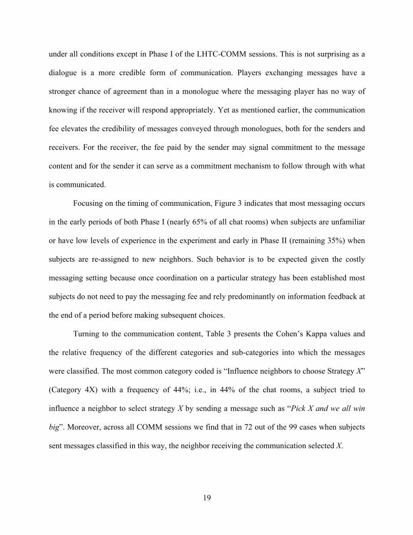
Turning to the communication content, Table 3 presents the Cohen’s Kappa values and

the relative frequency of the different categories and sub-categories into which the messages

were classified. The most common category coded is “Influence neighbors to choose Strategy X”

(Category 4X) with a frequency of 44%; i.e., in 44% of the chat rooms, a subject tried to

influence a neighbor to select strategy X by sending a message such as “Pick X and we all win

big”. Moreover, across all COMM sessions we find that in 72 out of the 99 cases when subjects

sent messages classified in this way, the neighbor receiving the communication selected X.

20  

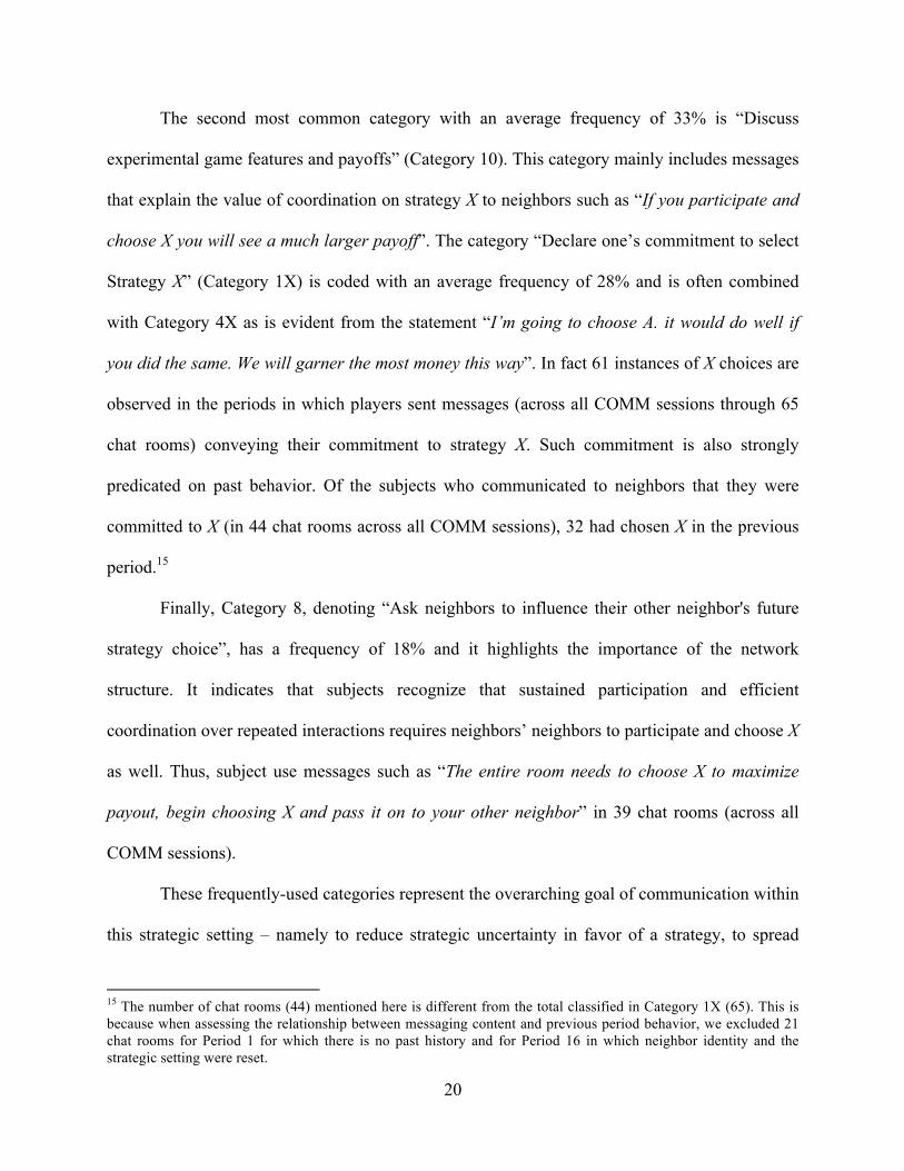
The second most common category with an average frequency of 33% is “Discuss

experimental game features and payoffs” (Category 10). This category mainly includes messages

that explain the value of coordination on strategy X to neighbors such as “If you participate and

choose X you will see a much larger payoff”. The category “Declare one’s commitment to select

Strategy X” (Category 1X) is coded with an average frequency of 28% and is often combined

with Category 4X as is evident from the statement “I’m going to choose A. it would do well if

you did the same. We will garner the most money this way”. In fact 61 instances of X choices are

observed in the periods in which players sent messages (across all COMM sessions through 65

chat rooms) conveying their commitment to strategy X. Such commitment is also strongly

predicated on past behavior. Of the subjects who communicated to neighbors that they were

committed to X (in 44 chat rooms across all COMM sessions), 32 had chosen X in the previous

period.15

Finally, Category 8, denoting “Ask neighbors to influence their other neighbor's future

strategy choice”, has a frequency of 18% and it highlights the importance of the network

structure. It indicates that subjects recognize that sustained participation and efficient

coordination over repeated interactions requires neighbors’ neighbors to participate and choose X

as well. Thus, subject use messages such as “The entire room needs to choose X to maximize

payout, begin choosing X and pass it on to your other neighbor” in 39 chat rooms (across all

COMM sessions).

These frequently-used categories represent the overarching goal of communication within

this strategic setting – namely to reduce strategic uncertainty in favor of a strategy, to spread

                                                                                                                         15 The number of chat rooms (44) mentioned here is different from the total classified in Category 1X (65). This is because when assessing the relationship between messaging content and previous period behavior, we excluded 21 chat rooms for Period 1 for which there is no past history and for Period 16 in which neighbor identity and the strategic setting were reset.

21  

information about the benefits of choosing a particular strategy, and to generate sustained

commitment for that strategy. The choice data confirm that communication is successful because

relative to NO-COMM settings, little negative time trend exists in participation rates (Figure 1

bottom panel) and a weak or no time trend exists for X choices conditional on participation

(bottom panel of Figure II in Appendix A). Despite the obvious value of communication to

promote coordination, however, 17 (out of 64) individuals never communicate. These individuals

sometimes received messages from neighbors and could have also used feedback information

about neighbors’ behavior at the end of a period to guide their behavior towards participation and

efficient coordination.

To evaluate the impact of transaction costs on participation in the presence of

communication opportunities, we analyze participation decisions using 2-way clustered logit

regressions for both phases. The dependent variable is the likelihood of participation in a period.

The control variable is the dummy variable taking a value of 1 for the high cost sessions.16 The

standard errors are clustered by subject and period (Cameron et al. 2012). The regression results

are presented in Model (1) and Model (2) of Table 4 and suggest no significant transaction cost

treatment effect in Phase I and a negative and significant effect in Phase II at 1% significance

level. This result provides partial support (in Phase II only) for Hypothesis I for the COMM

treatment. Note that this result contrasts with the finding in the NO-COMM treatment, where the

treatment effect is found in Phase I only.

In the COMM treatment subjects use communication to encourage their neighbors to

participate, to generate commitment for choosing the efficient strategy, and to ensure that the

willingness to participate and the commitment to choose X is passed on to other parts of the local

network through direct and indirect neighbor linkages. This implies that in Phase I                                                                                                                          16 We do not control for learning effects since Figure 1 (bottom panel) does not indicate any trend in the data.  

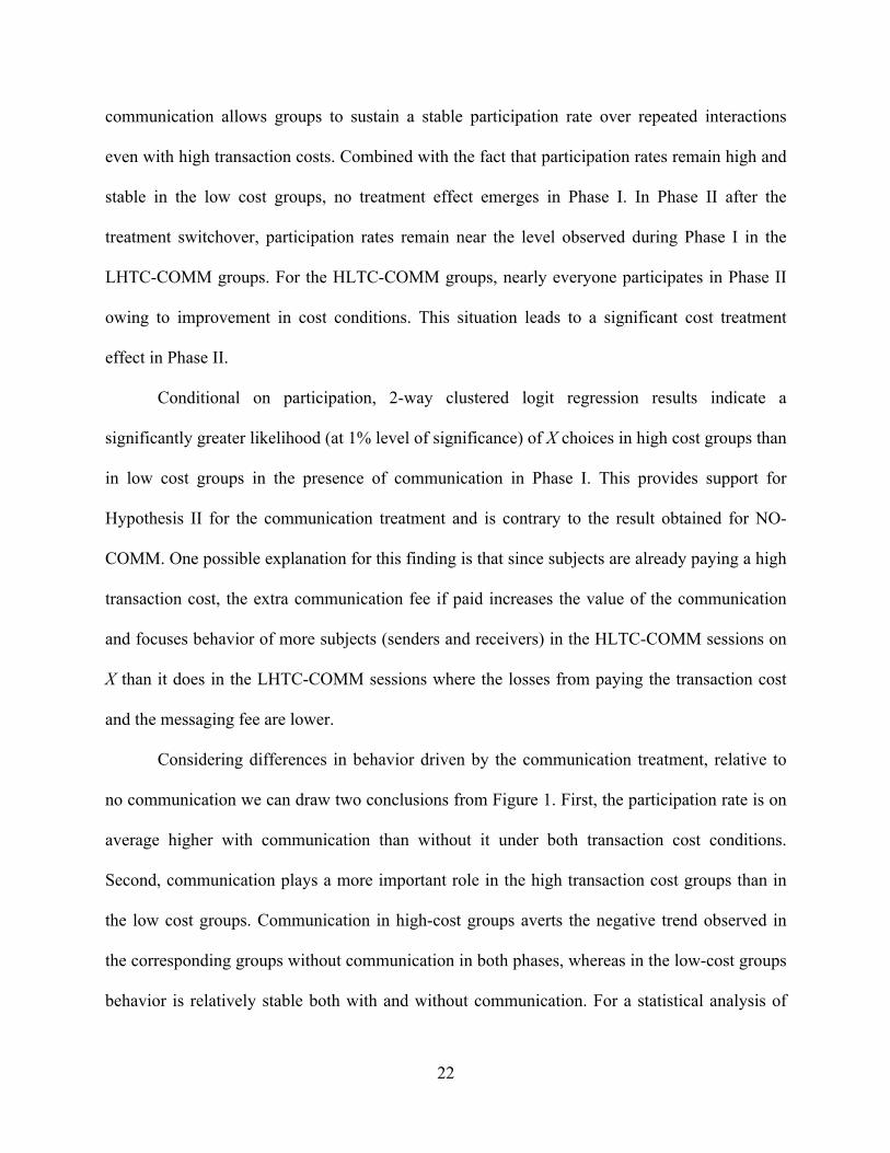
22  

communication allows groups to sustain a stable participation rate over repeated interactions

even with high transaction costs. Combined with the fact that participation rates remain high and

stable in the low cost groups, no treatment effect emerges in Phase I. In Phase II after the

treatment switchover, participation rates remain near the level observed during Phase I in the

LHTC-COMM groups. For the HLTC-COMM groups, nearly everyone participates in Phase II

owing to improvement in cost conditions. This situation leads to a significant cost treatment

effect in Phase II.

Conditional on participation, 2-way clustered logit regression results indicate a

significantly greater likelihood (at 1% level of significance) of X choices in high cost groups than

in low cost groups in the presence of communication in Phase I. This provides support for

Hypothesis II for the communication treatment and is contrary to the result obtained for NO-

COMM. One possible explanation for this finding is that since subjects are already paying a high

transaction cost, the extra communication fee if paid increases the value of the communication

and focuses behavior of more subjects (senders and receivers) in the HLTC-COMM sessions on

X than it does in the LHTC-COMM sessions where the losses from paying the transaction cost

and the messaging fee are lower.

Considering differences in behavior driven by the communication treatment, relative to

no communication we can draw two conclusions from Figure 1. First, the participation rate is on

average higher with communication than without it under both transaction cost conditions.

Second, communication plays a more important role in the high transaction cost groups than in

the low cost groups. Communication in high-cost groups averts the negative trend observed in

the corresponding groups without communication in both phases, whereas in the low-cost groups

behavior is relatively stable both with and without communication. For a statistical analysis of

23  

these claims, we employ 4 clustered logit regressions (one for each Phase and transaction cost

condition). The dependent variable is again the likelihood of participation, which is regressed on

a dummy variable equal to 1 for the COMM sessions, the reciprocal of the Period variable to

control for learning and capture the time trends, and an interaction term between these two

variables to account for differences in learning rates between treatments. All standard errors are

clustered by subject and period. Table 5 presents the results in Models (1) through (4).

A positive and significant estimate (at the 1% level) is obtained for the communication

treatment dummy variable in both phase regressions for the high cost condition and for Phase II

of the low cost treatment, providing partial support for Hypothesis III(a). Thus, while incurring

an additional transaction cost for the subjects who choose to message (and 47 subjects do so at

various points during the experiment), communication resolves the strategic uncertainty of many

more subjects in the COMM sessions leading to more X choices. The positive estimate for the

reciprocal of the period variable and the negative estimate for the interaction term for both

phases of the high-cost treatment and Phase I of the low-cost treatment signify the impact of

experience on participation. Thus, relative to no-communication scenarios, communication has

an unambiguously positive effect under unfavorable participation conditions and its benefits

under low-cost conditions are obtained only when subjects have had no prior experience with

participation in the AB scheme. To summarize:

Result 3: Communication generates greater rates of participation in the AB scheme.

Communication has a greater positive impact when compared to the no-communication setting

in high-cost groups at all levels of subject experience than in low-cost groups.

24  

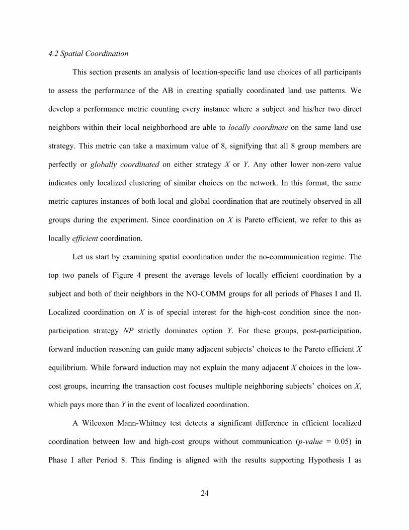
4.2 Spatial Coordination

This section presents an analysis of location-specific land use choices of all participants

to assess the performance of the AB in creating spatially coordinated land use patterns. We

develop a performance metric counting every instance where a subject and his/her two direct

neighbors within their local neighborhood are able to locally coordinate on the same land use

strategy. This metric can take a maximum value of 8, signifying that all 8 group members are

perfectly or globally coordinated on either strategy X or Y. Any other lower non-zero value

indicates only localized clustering of similar choices on the network. In this format, the same

metric captures instances of both local and global coordination that are routinely observed in all

groups during the experiment. Since coordination on X is Pareto efficient, we refer to this as

locally efficient coordination.

Let us start by examining spatial coordination under the no-communication regime. The

top two panels of Figure 4 present the average levels of locally efficient coordination by a

subject and both of their neighbors in the NO-COMM groups for all periods of Phases I and II.

Localized coordination on X is of special interest for the high-cost condition since the non-

participation strategy NP strictly dominates option Y. For these groups, post-participation,

forward induction reasoning can guide many adjacent subjects’ choices to the Pareto efficient X

equilibrium. While forward induction may not explain the many adjacent X choices in the low-

cost groups, incurring the transaction cost focuses multiple neighboring subjects’ choices on X,

which pays more than Y in the event of localized coordination.

A Wilcoxon Mann-Whitney test detects a significant difference in efficient localized

coordination between low and high-cost groups without communication (p-value = 0.05) in

Phase I after Period 8. This finding is aligned with the results supporting Hypothesis I as

25  

presented in the discussion on participation. Since participation is significantly lower in the

HLTC-NO-COMM sessions, so is overall AB performance. A likely reason for any significant

difference appearing after Period 8 is that in the initial periods subjects are unfamiliar with the

strategic environment, so most X choices are either non-adjacent or involve only two neighbors

selecting X.

With repeated interactions, participation rates fall in both groups, but they fall more

steeply in the high-cost sessions (as an increasing number of subject’s strategic uncertainty gets

resolved in favor of NP) causing fewer neighbors to choose X. As a result, rates of localized

efficient coordination fall to about 14% in Period 15 in HLTC-NO-COMM groups. Performance

is maintained between 40% and 50% in the LHTC-NO-COMM groups, where more people

choose X and the participation rate has a weak negative trend, leading to the significant treatment

effect. In Phase II there is no significant difference across transaction cost treatments, consistent

with the previous result regarding no significant difference in participation rates.

Figure 5 presents the fraction of instances of globalized efficient coordination for the

NO-COMM sessions, defined as all eight group members choosing X. Wilcoxon Mann-Whitney

tests indicate no significant cost-treatment effect in either Phase. Group-level coordination is

difficult – for any value of the transaction cost, it is challenging to get all group members to

make the same choices, especially given that information feedback is limited to direct neighbors.

Yet positive rates of global coordination suggest that, despite participation challenges, the AB

scheme can sometimes fully coordinate environmentally-beneficial choices.

Result 4: Greater transaction costs reduce localized efficient coordination only for

inexperienced groups and globalized efficient coordination is not significantly impacted by

26  

variation in the transaction cost values.

Let us now compare rates of spatial coordination with communication. The bottom panel

of Figure 4 shows the percentage of localized coordination in the COMM groups by transaction

cost and for both phases. A surprising result is that in Phase I, localized coordination is greater in

the HLTC-COMM groups relative to the LHTC-COMM groups. This difference is marginally

significant at the 10% level on the basis of a 2-way clustered logit regression (Table 4, Model

(3)) where the dependent variable takes a value of one when players within a local neighborhood

are able to coordinate on the efficient strategy X and 0 otherwise. The independent variables are

the high cost treatment dummy and the reciprocal of the period variable included to capture non-

linear rates of learning. Thus, although in Phase I there is no support for Hypothesis I (as there is

no difference in the number of individuals who participate under the two cost conditions), more

neighboring players participate in HLTC-COMM groups than in LHTC-COMM groups.

Localized coordination is improved in low-cost groups in Phase II relative to high-cost groups

since virtually every individual in the HLTC-COMM group participates (reinforcing the

significant treatment effect supporting Hypothesis I) and nearly everyone chooses X. Model (4)

in Table 4 shows that this difference is statistically significant at the 1% level on the basis of a 2-

way clustered logit regression.17

Finally, we compare localized coordination rates with and without communication.

Models (5) through (8) in Table 5 present the results of four 2-way clustered logit regressions

(for each Phase and transaction cost condition). The dependent variable takes a value of one

when players within a local neighborhood are able to coordinate and choose X. Similar to the                                                                                                                          17  2-way clustered logit regressions (with every group being the unit of observation) indicate no significant effect of transaction costs on likelihood of global efficient coordination in the presence of communication (the data pooled across all sessions are presented in Figure 5).

27  

previous models, the control variables include a dummy variable taking a value of 1 for the

COMM sessions, the reciprocal of the period variable and an interaction term. Results indicate a

significant (at the 1% level) and positive estimate for the COMM dummy variable in both phase

regressions for the high transaction cost condition and for the low-cost condition in Phase II,

substantiating the information presented in Figure 4 when comparing across top and bottom

panels for each cost condition and phase.

Relative to the no-communication settings, messaging can guide behavior of a greater

number of adjacent individuals to the efficient choice, hence significantly improving the

likelihood of localized efficient coordination. For groups facing low transaction costs, the

COMM dummy variable is not significant in Phase I which is in line with Result 3. Moreover,

the signs of the significant estimates for the interaction term and the reciprocal of the period

variable for the high-cost models indicate that repeated interactions improve performance in

groups with communication. Since the negative trend is largely a result of strategic uncertainty

being resolved in favor of NP and communication reduces strategic uncertainty in favor of

participation and X, this result follows automatically. This finding supports Hypothesis III(b) and

underscores the positive role of communication (even though it adds to the transaction cost

incurred) in guiding the selection of the efficient Nash equilibrium outcome in coordination

games with both Pareto-dominant and risk-dominant Nash equilibria within a local network.

Result 5: Mechanisms to reduce strategic uncertainty, such as communication, can build

commitment for choosing the efficient strategy and improve AB performance in the presence of

transaction costs.

28  

5. Discussion

Our study results are of course predicated on the nature of the strategic environment, i.e.,

the payoff functions under either high or low transaction costs, the size and circular nature of the

local network, and the degree of information feedback. A circular network does not describe

many real world settings where an AB policy could be introduced. Using a spatial set-up

different from the circular network (such as a line or lattice) may produce different results, since

some individuals would have different numbers of neighbors, and would therefore face different

levels of strategic uncertainty and payoffs. In the context of coordination games, Cassar (2007)

finds that the frequency of payoff-dominant choices is higher in a “small world” or a “random”

network than in a local network such as the one we consider. She also finds that coordination is

obtained much faster in the small world setting, while noting that “a theory linking network

characteristics to individual behavior is not yet available” (page 228). However, compared to

networks where strategic uncertainty varies across players, we could argue that the circular

network provides a lower bound on coordination failure in an AB setting.

We could have chosen a transaction cost value less than 40, which would not have made

Y strictly dominated by NP. We conjecture that this would lead to much greater participation and

many more Y choices than is currently observed under the high-cost treatment. While this is

interesting, this finding is similar to results obtained in Banerjee et al. 2014 and could have

eliminated (i) any difference between high-cost and low-cost groups and (ii) subjects’ ability to

use forward induction to guide their behavior in our network AB coordination game. Moreover,

the transaction cost treatment is more interesting if it generates differences in the set of equilibria

compared to when it just produces a difference in net payoffs. This leads to an interesting

thought experiment: if a regulator wishes to increase participation or efficient localized

29  

coordination in an AB scheme for a given budget, is it better to spend this money on increasing

the baseline (participation) subsidy, or on subsidizing the transactions costs that participants face

(e.g. by providing free advice)? In our experiment, no real difference exists in the effects of these

actions if the subsidy increase is equivalent for schemes X and Y, other than in the framing of the

payments. But targeting the baseline subsidy increase at X only could increase the uptake of this

land use relative to Y or non-participation by more than an equivalent reduction in transactions

costs. Unfortunately, we were unable to test whether significant differences in desired spatial

coordination emerge from such re-allocation of funds in the lab.

The size of the circular network and nature of information feedback may also impact

behavior. More information and smaller group sizes usually generate greater rates of efficient

choices in coordination games. However, with a group size of 8 we believe we have struck a

reasonable middle ground whereby the group is small enough for many individuals to choose X

and large enough for many to select NP or Y (owing to high strategic uncertainty). With this

group size we are able to assess the extent to which the AB can still deliver on its environmental

goal when the effect of each individual is relatively small compared to the total group. Finally,

we could have provided information to subjects beyond their local neighborhoods (e.g., on their

indirect neighbors such as in Banerjee et al., 2014). Although this would be inconsistent with our

localized communication format, it provides an avenue for future research especially if

regulatory agencies start publicly announcing enrollment rates in order to promote greater

participation. It is also possible that coordination failure would have implications for what

participants consider “fair”, and this could influence the likelihood of coordination on the Pareto-

superior equilibrium, especially if outcomes are observable such as in Reeson et al. (2011).

30  

6. Conclusions

PES schemes are increasingly being implemented as policy mechanisms to enhance the

supply of ecosystem services. The predominant property rights regime in countries such as the

US, the UK, New Zealand and Australia requires that landowners be financially compensated to

encourage the supply of ecosystem services, rather than being compelled to do so by regulation:

the “provider gets” principle (Hanley et al. 1998). Second, for many environmental outcomes,

spatial coordination increases the size of environmental benefits for a given level of enrollment

in voluntary conservation programs. The policy design challenge is to find systems of incentives

that spatially coordinate a voluntary sign-up program. The Agglomeration Bonus (AB) is one

such mechanism. However, the AB faces a number of potential problems, including the tendency

over time for participants to converge on risk-dominant outcomes, a lack of cost-effectiveness,

and, like many incentive programs, the size and nature of transaction costs. To date, the effects

of transactions costs have not been investigated in the AB literature, despite their importance to

PES scheme participation decisions.

In this paper we use a laboratory experiment to investigate how private transaction costs

affect the degree of participation in an AB scheme, its efficiency and the patterns of spatial

coordination in the presence and absence of communication. Results show that higher transaction

costs lead to greater non-participation, whilst lower transaction costs are conducive to producing

a greater degree of coordination on the most preferred environmental outcome. Full coordination

on the most efficient outcome is rarely achieved, but localized clusters of coordinated

conservation actions emerge in most cases.

Communication is costly and thus adds to the transaction costs incurred, but it improves

outcomes, generating economic and environmental benefits. There are clear parallels here with

31  

experimental findings on the implications of communication (albeit costless) in “ambient”

pollution tax schemes (Segerson 1988), where the pollution tax liability of each firm depends on

group behavior. For example, Suter et al. (2008) find that allowing participants to communicate

in a non-binding fashion produces lower pollution levels and maximizes group profits. Our

communication results can also be compared with the effects of costless communication in

experiments on Voluntary Contribution Mechanisms for public goods, such as in Isaac and

Walker (1988), where non-binding group discussion significantly reduced free-riding behavior.

The policy implications of our results are clear: if the regulator can design an AB scheme

in a way which keeps transaction costs low relative to the payoffs of coordination, then it will be

easier to achieve spatial coordination (both locally and globally). This, in turn, enhances a more

effective delivery of ecosystem services. However, if achieving a given environmental objective

requires writing (complicated) rules for potential participants, then there is a trade-off between

improving environmental effectiveness and increasing coordination, since such complications

will increase transactions costs. Set against this scenario, facilitating low-cost communication

between landowners would improve the likelihood of successful coordination towards socially-

desirable land use patterns. Providing subsidies to lower transaction costs initially would also

foster early coordination, and our results suggest that improved performance could persist even

after such subsidies are removed and transaction costs increase.

 

 

32  

References

Armsworth, Paul R., Szvetlana Acs, Martin Dallimer, Kevin J. Gaston, Nick Hanley, and Paul Wilson. 2012. The cost of policy simplification in conservation incentive programs. Ecology Letters 15 (5): 406-14.

Banerjee, Simanti, Nick Hanley, Frans P. deVries, and Daan P. van Soest. 2014. The impact of information provision on agglomeration bonus performance: An experimental study on local networks. American Journal of Agricultural Economics 96 (4): 1009-29.

Banerjee, Simanti, Anthony M. Kwasnica, and James S. Shortle. 2012. Agglomeration bonus in small and large local networks: A laboratory examination of spatial coordination. Ecological Economics 84 (12): 142-52.

Berninghaus, Siegfried K., Karl-Martin Ehrhart, and Claudia Keser. 2002. Conventions and local interaction structures: Experimental evidence. Games and Economic Behavior 39 (2): 177-205.

Cachon, Gérard P., and Colin F. Camerer. 1996. Loss-avoidance and forward induction in experimental coordination games. The Quarterly Journal of Economics 111 (1) (Feb.): 165-94.

Cameron, A. Colin, Jonah B. Gelbach, and Douglas L. Miller. 2012. Robust inference with multiway clustering. Journal of Business & Economic Statistics 29 (2): 238-49.

Cason, Timothy N., and Leigh Raymond. 2011. Framing effects in an emissions trading experiment with voluntary compliance. In Experiments on energy, the environment, and sustainability (Research in Experimental Economics, Volume 14)., eds. R. Mark Isaac, Douglas A. Norton, 77-114: Emerald Group Publishing Limited.

Cassar, Alessandra. 2007. Coordination and cooperation in local, random and small world networks: Experimental evidence. Games and Economic Behavior 58 (2): 209-30.

Claassen, Roger, and Marc Ribaudo. 2016. Cost-effective conservation programs for sustaining environmental quality. Choices 31 (3).

Cohen, Jacob. 1960. A coefficient of agreement for nominal scales. Educational and Psychological Measurement 20: 37-46.

Conservation Stewardship Program, Natural Resources Conservation Service, 2016. http://www.nrcs.usda.gov/wps/portal/¬/main/national/programs/financial/csp/ Accessed July 27, 2016

Cooper, Russell, Douglas V. DeJong, Robert Forsythe, and Thomas W. Ross. 1989. Communication in the battle of the sexes game: Some experimental results. The Rand Journal of Economics 20 (4) (Winter): 568-87.

Cooper, Russell, Douglas V. DeJong, Robert Forsythe, and Thomas W. Ross. 1994. Alternative institutions for resolving coordination problems: Experimental evidence on forward induction and pre-play communication. In Problems of coordination in economic activity, ed. James Friedman, 129-146. New York: Springer.

33  

Cooper, Tamsin, Kaley Hart, and David Baldock. 2009. Provision of public goods through agriculture in the European Union. Institute for European Environmental Policy London.

Dallimer, M., K. J. Gaston, A. M. Skinner, N. Hanley, S. Acs, and P. R. Armsworth. 2010. Field-level bird abundances are enhanced by landscape-scale agri-environment scheme uptake. Biology Letters 6 (5) (Oct 23): 643-6.

Devetag, Giovanna. 2003. Coordination and information in critical mass games: An experimental study. Experimental Economics 6 (1): 53-73.

Dufwenberg, Martin, Gunnar Köhlin, Peter Martinsson, and Haileselassie Medhin. 2016. Thanks but no thanks: A new policy to reduce land conflict. Journal of Environmental Economics and Management 77 (1): 31-50.

Engel, Stefanie, Stefano Pagiola, and Sven Wunder. 2008. Designing payments for environmental services in theory and practice: An overview of the issues. Ecological Economics 65 (4) (5/1): 663-74.

Falconer, Katherine, and Caroline Saunders. 2002. Transaction costs for SSSIs and policy design. Land use Policy 19 (2): 157-66.

Fischbacher, Urs. 2007. Z-tree: Zurich toolbox for ready-made economic experiments. Experimental Economics 10: 171.

Fooks, Jacob R., Nathaniel Higgins, Kent D. Messer, Joshua M. Duke, Daniel Hellerstein, and Lori Lynch. 2016. Conserving spatially explicit benefits in ecosystem service markets: Experimental tests of network bonuses and spatial targeting. American Journal of Agricultural Economics 98 (2): 468-88.

Greiner, Ben. 2015. Subject pool recruitment procedures: Organizing experiments with ORSEE. Journal of the Economic Science Association 1 (1): 114-25.

Hanley, Nick, Simanti Banerjee, Gareth D. Lennox, and Paul R. Armsworth. 2012. How should we incentivize private landowners to ‘produce’ more biodiversity? Oxford Review of Economic Policy 28 (1): 93-113.

Hanley, Nick, Hilary Kirkpatrick, Ian Simpson, and David Oglethorpe. 1998. Principles for the provision of public goods from agriculture: Modeling moorland conservation in Scotland. Land Economics: 102-13.

Hanley, Nick, and Ben White. 2014. Incentivizing the provision of ecosystem services. International Review of Environmental and Resource Economics 7 (3-4): 299-331.

Harsanyi, John C., and Reinhard Selten. 1988. A general theory of equilibrium selection in games. MIT Press Books 1.

Isaac, R. Mark, and James M. Walker. 1988. Communication and free-­‐riding behavior: The voluntary contribution mechanism. Economic Inquiry 26 (4): 585-608.

34  

Jackson, Matthew O. 2010. Social and economic networks. Vol. 3. Princeton: Princeton University Press.

Kampas, Athanasios, and Ben White. 2004. Administrative costs and instrument choice for stochastic non-point source pollutants. Environmental and Resource Economics 27 (2): 109-33.

Krippendorff, Klaus. 2004. Content analysis: An introduction to its methodology. Sage.

Kuhfuss, Laure, Raphaële Préget, Sophie Thoyer, and Nick Hanley. 2016. Nudging farmers to enroll land into agri-environmental schemes: The role of a collective bonus. European Review of Agricultural Economics 43 (4): 609-36.

Landis, J. Richard, and Gary G. Koch. 1977. An application of hierarchical kappa-type statistics in the assessment of majority agreement among multiple observers. Biometrics: 363-74.

Lane, Stuart N., Chris J. Brookes, Mike J. Kirkby, and Joseph. Holden. 2004. A network-­‐index-­‐based version of TOPMODEL for use with high-­‐resolution digital topographic data. Hydrological Processes 18 (1): 191-201.

Lane, Stuart N., Chris J. Brookes, A. Louise Heathwaite, and Sim Reaney. 2006. Surveillant science: Challenges for the management of rural environments emerging from the new generation diffuse pollution models. Journal of Agricultural Economics 57 (2): 239-57.

Lawley, Chad, and Wanhong Yang. 2015. Spatial interactions in habitat conservation: Evidence from prairie pothole easements. Journal of Environmental Economics and Management 71 (5): 71-89.

McCann, Laura, Bonnie Colby, K. William Easter, Alexander Kasterine, and K. V. Kuperan. 2005. Transaction cost measurement for evaluating environmental policies. Ecological Economics 52 (4) (3/1): 527-42.

Merckx, Thomas, Ruth E. Feber, Philip Riordan, Martin C. Townsend, Nigel A. D. Bourn, Mark S. Parsons, and David W. Macdonald. 2009. Optimizing the biodiversity gain from agri-environment schemes. Agriculture, Ecosystems & Environment 130 (3–4) (4): 177-82.

Mettepenningen, Evy, Ann Verspecht, and Guido Van Huylenbroeck. 2009. Measuring private transaction costs of European agri-environmental schemes. Journal of Environmental Planning and Management 52 (5): 649-67.

Önal, Hayri, and Robert A. Briers. 2006. Optimal selection of a connected reserve network. Operations Research 54 (2): 379-88.

Parkhurst, Gregory M., and Jason F. Shogren. 2007. Spatial incentives to coordinate contiguous habitat. Ecological Economics 64 (2): 344-55.

Parkhurst, Gregory M., Jason F. Shogren, Chris Bastian, Paul Kivi, Jennifer Donner, and Rodney BW Smith. 2002. Agglomeration bonus: An incentive mechanism to reunite fragmented habitat for biodiversity conservation. Ecological Economics 41 (2): 305-28.

Plott, Charles R., and Dean V. Williamson. 2000. Markets for contracts: Experiments exploring the compatibility of games and markets for games. Economic Theory 16 (3): 639-60.

35  

Reeson, Andrew F., Luis C. Rodriguez, Stuart M. Whitten, Kristen Williams, Karel Nolles, Jill Windle, and John Rolfe. 2011. Adapting auctions for the provision of ecosystem services at the landscape scale. Ecological Economics 70 (9) (7/15): 1621-7.

Romero, Julian. 2015. The effect of hysteresis on equilibrium selection in coordination games. Journal of Economic Behavior & Organization 111 (0) (3): 88-105.

Segerson, Kathleen. 1988. Uncertainty and incentives for nonpoint pollution control. Journal of Environmental Economics and Management 15 (1): 87-98.

Shortle, James S., David G. Abler, and Richard D. Horan. 1998. Research issues in nonpoint pollution control. Environmental and Resource Economics 11 (3-4): 571-85.

Shortle, James S., Marc Ribaudo, Richard D. Horan, and David Blandford. 2012. Reforming agricultural nonpoint pollution policy in an increasingly budget-constrained environment. Environmental Science & Technology 46 (3): 1316-25.

Suter, Jordan F., Christian A. Vossler, Gregory L. Poe, and Kathleen Segerson. 2008. Experiments on damage-based ambient taxes for nonpoint source polluters. American Journal of Agricultural Economics 90 (1): 86-102.

Van Huyck, John B., Raymond C. Battalio, and Richard O. Beil. 1993. Asset markets as an equilibrium selection mechanism: Coordination failure, game form auctions, and tacit communication. Games and Economic Behavior 5 (3) (7): 485-504.

Warziniack, Travis, Jason F. Shogren, and Gregory Parkhurst. 2007. Creating contiguous forest habitat: An experimental examination on incentives and communication. Journal of Forest Economics 13 (2): 191-207.

Wätzold, Frank, Melanie Mewes, Rob van Apeldoorn, Riku Varjopuro, Tadeusz Jan Chmielewski, Frank Veeneklaas, and Marja-Leena Kosola. 2010. Cost-effectiveness of managing Natura 2000 sites: An exploratory study for Finland, Germany, the Netherlands and Poland. Biodiversity and Conservation 19 (7): 2053-69.

Williams, Justin C., Charles S. ReVelle, and Simon A. Levin. 2005. Spatial attributes and reserve design models: A review. Environmental Modeling & Assessment 10 (3): 163-81.

Windle, Jill, John Rolfe, Juliana McCosker, and Andrea Lingard. 2009. A conservation auction for landscape linkage in the southern desert uplands, Queensland. The Rangeland Journal 31 (1): 127-35.

Wunder, Sven. 2007. The efficiency of payments for environmental services in tropical conservation; la eficiencia de los pagos por servicios ambientales en la conservación trópicos. Conservation Biology 21 (1): 48-58.  

 

36  

TABLES  

Table 1a: Payoff Table for High Transaction Cost condition

Payoff Table

Actions Chosen by Neighbors

Your Action Both

Participate Choose X

Both Participate

and one Chooses X & other Y

Both Participate

and Choose Y

Only one Participates & Chooses

X

Only one Participates & Chooses

Y

No Neighbor

Participates

X 210 125 40 125 40 40 Y 145 155 165 145 155 145

NP (Non-Participation) 175 175 175 175 175 175

Table 1b: Payoff Table for Low Transaction Cost condition

Payoff Table

Actions Chosen by Neighbors

Your Action Both

Participate Choose X

Both Participate

& one Chooses X & other Y

Both Participate & Choose

Y

Only one Participates & Chooses

X

Only one Participates & Chooses

Y

No Neighbor

Participates

X 235 150 65 150 65 65 Y 170 180 190 170 180 170

NP (Non-Participation) 175 175 175 175 175 175

Table 2: Summary of Experimental Design

Communication Treatment

Transaction Cost Ordering Treatment No-Comm Comm

High-Low HLTC-No-Comm (8 sessions)

HLTC-Comm (4 sessions)

Low-High LHTC-No-Comm (8 sessions)

LHTC-Comm (4 sessions)

37  

Table 3: Categories for coding messages (reaching at least Moderate Reliability) and

observed frequency in chat rooms

+ Only those categories (and sub-categories) reaching an agreement of Moderate or higher reliability are listed. X and Y labels correspond to Strategies A and B in the experiment. * Represents categories which have a relative frequency of coding of 15% or more.

Category+ Description Cohen’s Kappa

Relative Frequency of Coding

1 Declare one’s commitment to a particular strategy 1X Will select X 0.83 0.28* 1Y Will select Y 0.90 0.03 1NP Will select NP 0.75 0.06 2 Explain own reason for choosing a strategy (X, Y or NP) 2P In the past periods 0.45 0.02

3 Inform one neighbor about other neighbor’s strategy choice

3X Other neighbor chose X 0.45 0.03 3Y Other neighbor chose Y 0.79 0.03 3NP Other neighbor chose NP 0.69 0.04 3NX Other neighbor did not chose X 0.56 0.03 4 Influence neighbor(s) to select a particular strategy 4X Choose X 0.81 0.44* 4Y Choose Y 0.78 0.02 4NP Choose NP 0.79 0.01 5 Ask neighbors about their future choices 0.55 0.07 6 Ask neighbors about their reasons for choosing a strategy 0.65 0.03 7 Ask neighbors about their other neighbors past choices 0.53 0.02

8 Ask neighbors to influence their other neighbor's future strategy choice 0.88 0.18*

8X Influence other neighbor to select X 0.89 0.17 8Y Influence other neighbor to select Y 0.49 0.00 9 Refer to own past strategy choice 0.49 0.01 10 Discuss about experimental features & game payoffs 0.73 0.33* 11 Agree on a strategy 0.55 0.13 12 Other 0.54 0.34*

38  

Table 4: 2-way Clustered Logit Regressions for Participation and Performance Analysis in each Phase for Communication Groups

Dependent Variables Participation Localized Efficient Coordination

Independent Variables

Model 1 Model 2 Model 3 Model 4

Phase I Phase II Phase I Phase II High Transaction

Cost -0.024 (0.019)

-0.157** (0.032)

0.027* (0.015)

-0.106*** (0.023)

𝟏𝑷𝒆𝒓𝒊𝒐𝒅!

- - -1.343** (0.344)

-0.756** (0.048)

Constant 2.161** (0.612)

7.43** (1.15)

-0.098 (0.478)

1.975*** (0.49)

Number of observations 960 (480 in each Phase)

Cluster Variables Individual Subject and Experimental Period in a Phase

** Represents statistical significance at the 1% level, * at the 10% level + Period takes a value between 1 and 15 Table 5: 2-way Clustered Logit Regressions for Performance comparison of Communication and No Communication Treatments by Phase and Transaction Cost#

Independent Variables

Participation Localized Efficient Coordination

Model 1: Phase I (HC)

Model 2: Phase II

(LC)

Model 3: Phase I

(LC)

Model 4: Phase II

(HC)

Model 5: Phase I (HC)

Model 6: Phase II

(LC)

Model 7: Phase I

(LC)

Model 8: Phase II

(HC)

Comm 0.892*** (0.229)

1.999*** (0.622)

0.197 ( 0.245)

0.782*** (0.246)

1.063*** (0.221)

2.019*** (0.374)

0.028 (0.192)

0.864*** (0.237)

𝟏𝑷𝒆𝒓𝒊𝒐𝒅!

2.197** (0.871)

0.428 (0.421)

1.960*** ( 0.652)

2.674*** (0.902)

0.027 (0.458)

-0.368 (0.227)

-1.152*** (0.381)

0.610** (0.252)

𝟏𝑷𝒆𝒓𝒊𝒐𝒅!

 

x  Comm  

-1.060** (-0.467)

-1.094 (0.81)

-1.285*** (0.356)

-1.179*** (0.489)

-0.848** (0.368)

-0.375 (0.658)

0.078 (0.327)

-0.652*** (0.095)

Constant -0.600** (0.29)

1.579*** (0.251)

1.549*** (0.29)

-0.5* (0.26)

-1.088*** (0.297)

-0.086 (0.728)

0.171 (0.449)

-0.546** (0.245)

Number of Observations 1440

Cluster Variables Individual Subject and Experimental Period in a Phase

# HC refers to High Transaction Cost and LC refers to Low Transaction Cost *** Represents statistical significance at the 1% level, ** at the 5% level and * at the 10% level + Period takes a value between 1 and 15

Figure 1: Fraction of Participation in Phase I & Phase II of No-Comm and Comm Sessions by Transaction Costs Treatment

0.95

0.7

0.78

0.2

0.86

0.8

0.78

0.36

0.81

0.75

0.88

0.72

0.97

0.81

0.97

0.75

0.2

.4.6

.81

0.2

.4.6

.81

0.2

.4.6

.81

0.2

.4.6

.81

1 2 3 4 5 6 7 8 9 10 11 12 13 14 15 16 17 18 19 20 21 22 23 24 25 26 27 28 29 30

1 2 3 4 5 6 7 8 9 10 11 12 13 14 15 16 17 18 19 20 21 22 23 24 25 26 27 28 29 30

No-Comm, Phase I No-Comm, Phase II

Comm, Phase I Comm, Phase II

Low Transaction Cost High Transaction Cost

Frac

tion

of P

artic

ipat

ion

Dec

isio

ns

Period

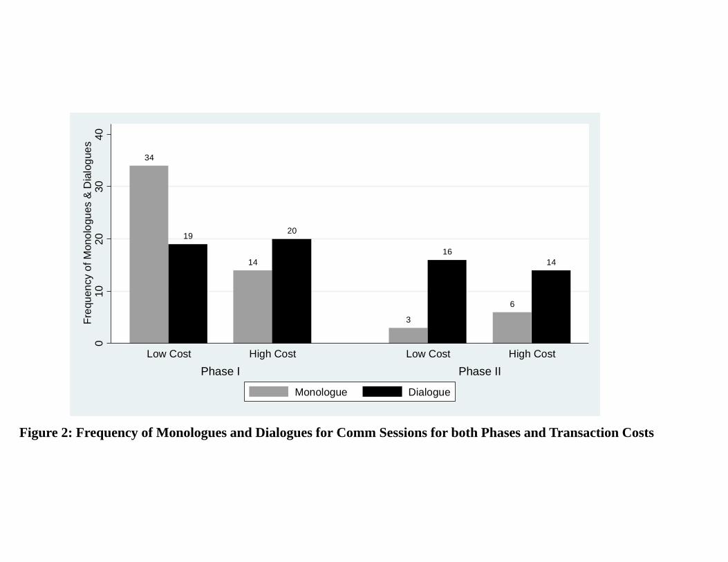
Figure 2: Frequency of Monologues and Dialogues for Comm Sessions for both Phases and Transaction Costs

34

19

14

20

3

16

6

14

010

2030

40Fr

eque

ncy

of M

onol

ogue

s &

Dia

logu

es

Phase I Phase IILow Cost High Cost Low Cost High Cost

Monologue Dialogue

Figure 3: Fraction and Timing of Communication Channels opened with One or Both Neighbors by Phase and Transaction Cost

0.2

.4.6

.81

0.2

.4.6

.81

1 2 3 4 5 6 7 8 9 10 11 12 13 14 15

16 17 18 19 20 21 22 23 24 25 26 27 28 29 30

Period

1 2 3 4 5 6 7 8 9 10 11 12 13 14 15

16 17 18 19 20 21 22 23 24 25 26 27 28 29 30

Period

Phase I: Low Transaction Cost

Phase II: Low Transaction Cost

Phase I: High Transaction Cost

Phase II: High Transaction Cost

Frac

tion

of A

vaila

ble

Com

mun

icat

ion

Cha

nnel

s O

pene

d

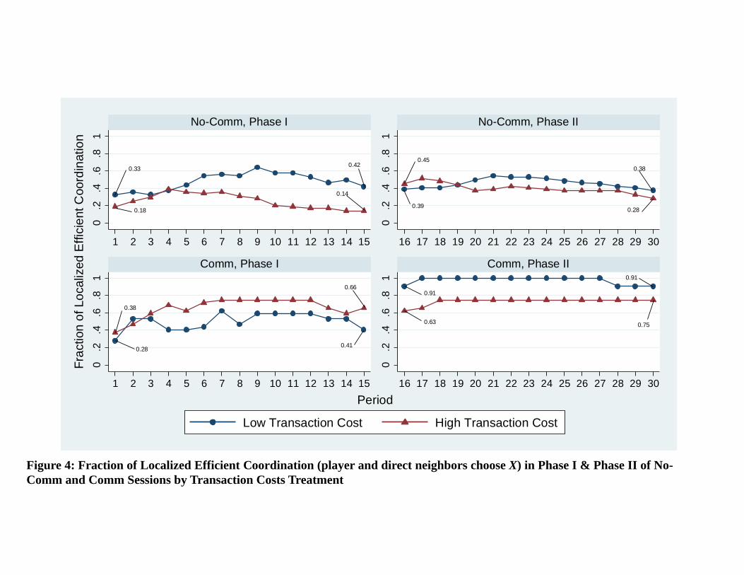
Figure 4: Fraction of Localized Efficient Coordination (player and direct neighbors choose X) in Phase I & Phase II of No-Comm and Comm Sessions by Transaction Costs Treatment

0.33

0.18

0.42

0.14

0.45

0.39

0.38

0.28

0.28

0.38

0.66

0.41

0.91

0.63

0.91

0.75

0.2

.4.6

.81

0.2

.4.6

.81

0.2

.4.6

.81

0.2

.4.6

.81

1 2 3 4 5 6 7 8 9 10 11 12 13 14 15 16 17 18 19 20 21 22 23 24 25 26 27 28 29 30

1 2 3 4 5 6 7 8 9 10 11 12 13 14 15 16 17 18 19 20 21 22 23 24 25 26 27 28 29 30

No-Comm, Phase I No-Comm, Phase II

Comm, Phase I Comm, Phase II

Low Transaction Cost High Transaction Cost

Frac

tion

of L

ocal

ized

Effi

cien

t Coo

rdin

atio

n

Period

Figure 5: Perfect/Global Efficient Coordination (the whole group chooses X) in all treatments for both Phases

0.27

0.15

0.35

0.48

0.31 0.33

0.93

0.72

0.2

.4.6

.81

Frac

tion

of G

loba

l Coo

rdin

atio

n

Phase I Phase IINo-Comm Comm No-Comm Comm

Low Transaction Cost High Transaction Cost

Figure I: Fraction of Choices Pooled over Time for All Treatments

0.64

0.21

0.14

0.45

0.04

0.51

0.82

0.110.07

0.76

0.00

0.24

0.2

.4.6

.81

Frac

tion

of C

hoic

es

No-Comm CommLow Cost High Cost Low Cost High Cost

X Y Non-Participation

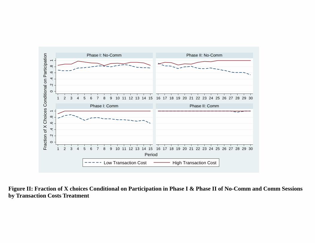
0.2

.4.6

.81

0.2

.4.6

.81

1 2 3 4 5 6 7 8 9 10 11 12 13 14 15 16 17 18 19 20 21 22 23 24 25 26 27 28 29 30

1 2 3 4 5 6 7 8 9 10 11 12 13 14 15 16 17 18 19 20 21 22 23 24 25 26 27 28 29 30

Phase I: No-Comm Phase II: No-Comm

Phase I: Comm Phase II: Comm

Low Transaction Cost High Transaction Cost

Frac

tion

of X

Cho

ices

Con

ditio

nal o

n P

artic

ipat

ion

Period

Figure II: Fraction of X choices Conditional on Participation in Phase I & Phase II of No-Comm and Comm Sessions by Transaction Costs Treatment

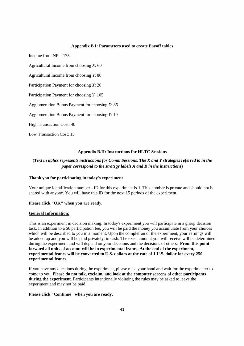
41

Appendix B.I: Parameters used to create Payoff tables

Income from NP = 175

Agricultural Income from choosing X: 60

Agricultural Income from choosing Y: 80

Participation Payment for choosing X: 20

Participation Payment for choosing Y: 105

Agglomeration Bonus Payment for choosing X: 85

Agglomeration Bonus Payment for choosing Y: 10

High Transaction Cost: 40

Low Transaction Cost: 15

Appendix B.II: Instructions for HLTC Sessions

(Text in italics represents instructions for Comm Sessions. The X and Y strategies referred to in the paper correspond to the strategy labels A and B in the instructions)

Thank you for participating in today's experiment Your unique Identification number - ID for this experiment is 1. This number is private and should not be shared with anyone. You will have this ID for the next 15 periods of the experiment. Please click "OK" when you are ready. General Information: This is an experiment in decision making. In today's experiment you will participate in a group decision task. In addition to a $6 participation fee, you will be paid the money you accumulate from your choices which will be described to you in a moment. Upon the completion of the experiment, your earnings will be added up and you will be paid privately, in cash. The exact amount you will receive will be determined during the experiment and will depend on your decisions and the decisions of others. From this point forward all units of account will be in experimental francs. At the end of the experiment, experimental francs will be converted to U.S. dollars at the rate of 1 U.S. dollar for every 250 experimental francs. If you have any questions during the experiment, please raise your hand and wait for the experimenter to come to you. Please do not talk, exclaim, and look at the computer screens of other participants during the experiment. Participants intentionally violating the rules may be asked to leave the experiment and may not be paid. Please click "Continue" when you are ready.

42

Today's Decision Making Task: The experiment will have thirty periods . In each period you will be in a group with 7 other participants. You and all the other players are arranged around a circle. The diagram of this circle is included in the handout that has been provided to you. The black dots on the circle represent your location. On this circle, you have two neighbors - a right or anti-clockwise neighbor and a left or clockwise neighbor. You will never know the identity of your neighbors. Your ID will determine who your neighbors are. Please keep in mind that every player has a different set of neighbors. Thus if you are Player 8 then your right or anti-clockwise neighbor is Player 7 and left or clockwise neighbor is Player 1. Similarly Player 7 has you as their left or clockwise neighbor and Player 6 as their right or anti-clockwise neighbor. Your ID and your neighbors will be the same for the first 15 periods of the experiment. At the beginning of Period 16, everyone will be provided with a different ID. As a result of this ID change, your neighbors between Periods 16 and 30 will be different from those between Periods 1 and 15. Also please remember that the person sitting at the computer terminal beside you is not your neighbor in the experiment. During this experiment each of you will assume the role of a landowner who can participate in a land management program or opt out of it. In both cases, you will receive money for your actions. You will first be given the option to participate in this program. If you choose not to participate, you will receive a payment. Participation is costly and so you have to incur a cost to do so. Once you have incurred the cost, you will be able to take part in a group decision task which is part of the land management program. In this task, you will make a choice between two types of land use actions denoted by A and B. You will receive a payment based on your choice of A or B. Since this is a group decision task, your payment will depend on the choices made by your neighbors as well. In a moment we will give you a detailed description of how your payment will be determined. Please note that you may decide to participate in the task but one or both of your neighbors may choose not to. Also while you decide to participate, you will not know what choices your neighbors' are making. Please raise your hand if there are any questions otherwise click "Continue". Your Payment from Group Decision Task: If you choose to participate in the land management program, then in each period of the experiment, the computer will display a table such as the one shown below. This Payoff Table will be the same for everyone during a period. However the values in the cells will be different in different periods of the experiment. You will be provided with a handout containing the Payoff Table. Each number in the table corresponds to a payment (in experimental francs) resulting from a possible combination of your choice of A or B (in the row) and your neighbors' choices (in the column). Please note that all figures in the table are net of the participation cost, i.e., the participation cost has already been deducted from the payoffs. For example, suppose the participation cost is 40 and your payoff from choosing A and both your neighbors participating and choosing A is 250. Then your final payoff is (250 - 40) = 210. This is listed in the first cell of the first row of the Payoff Table. Similarly if you select B after participation and only one of your neighbors participates and chooses B, the payoff is 195. Then your final payoff is (195 - 40) = 155. The last column in the table indicates your payoffs if you participate and none of your neighbors participate. Please note that when you will be asked to participate or not, you will know the value of the cost you have to incur. In general, your payoff from the group decision task increases when you choose the same action as your participating neighbors.

43

Also your payoffs are the same if 1) one or both neighbors participate and choose a different strategy than you or 2) they don't participate at all. For example, the payment to you from choosing B and both of your neighbors choosing A is the same as you choosing B and none of your neighbors participating. Communication stage: Before making a choice in a period about participating in the land management program, you will have the option to communicate with one or both of your neighbors. For every person you choose to communicate with, you have to pay a fee of 5 experimental francs per person. Thus if you choose to communicate with both neighbors, you have to pay a fee of 10 francs. If you choose not to communicate, you don't have to pay the fee. Please note that it is possible that you pay the fee and choose to communicate with your neighbors but they choose not to pay the fee and communicate with you. If that is the case, you will be able to send messages to the neighbors with whom you have paid to chat and they will be able to view these messages. Similarly, you may have chosen not to chat with your neighbors but one or both of them paid a fee to chat with you. They will be able to send messages to you which you will be able to view. Your communication with the neighbor(s) will consist of messages exchanged in "chat boxes" to the left and/or right of your computer screen depending upon which neighbor you chat with. Messages sent in this chat will only be viewed by you and the neighbor you send it to. For example, if you are Player 8 and you and both your neighbors have paid the fee to communicate, the chat box on your left will contain messages you send to and receive from Player 1 and that to the right will contain messages you send to and receive from Player 7. You will be able to send and receive chats for 60 seconds each period. In order to send a chat to your neighbors, please type in the blue panel at the bottom of your chat box and press Enter. To send a message to your left neighbor, type your chat in the left blue panel at the base of the left chat box. Similarly use the blue panel at the base of the right chat box to send chats to your right neighbor. Although the messages you send to each other will be recorded, your ID remains anonymous and hence all communication is anonymous to the experimenter and cannot be traced back to any subject. In sending messages, you should follow two basic rules: (1) be civil to one another and do not use profanities, (2) only use your ID to identify yourself in any manner. After the chat period is over you will be able to see the chats you have exchanged with your neighbors for 10 seconds. After these 10 seconds are over, everyone will make their participation and land management decisions. Please note that you do not learn the land management decisions of your neighbors while making your own decision. Making a choice in a period: (No-Comm) Once the period starts, each of you will first choose whether to participate or not. If you decide not to participate, then you will receive a fixed payoff. This payoff does not depend upon your neighbors' participation decisions. If you decide to participate, then in the next stage, you will choose strategy A or B by clicking on one of the buttons that will appear on the right of your screen. You may change your choice as often as you like, but once you click on OK your choice for that period is final. Note that when you are making a choice, you will not know what choices others are making. Also, remember that you will never know the identity of anyone else in your group, meaning that all choices are confidential and that no one will ever know what choices you make. At the end of each period after you have made your choices, your screen will display your choice and payoff. Information will also be provided about whether your neighbors participated and if they did, what

44

were their choices for that period. Information on your accumulated payment through the current period will also be provided. At the end of the experiment, you will receive the sum of your payments from all thirty periods converted to real dollars. This will be paid to you privately in cash. Before starting the experiment you will participate in a quiz on the next screen. Please note that you will not earn any money from participating in the quiz i.e. this is a non-paying period. Your answers in this quiz will not influence your final payoffs at the end of the experiment. Making a choice in a period: (Comm) Once the period starts and after you have made a decision to communicate (or not), each of you will first choose whether to participate or not. If you decide not to participate, then you will receive a fixed payoff. This payoff does not depend upon your neighbors' participation decisions. If you decide to participate, then in the next stage, you will choose strategy A or B by clicking on one of the buttons that will appear on the right of your screen. You may change your choice as often as you like, but once you click on OK your choice for that period is final. Note that when you are making a choice, you will not know what choices others are making. Also, remember that you will never know the identity of anyone else in your group, meaning that all choices are confidential and that no one will ever know what choices you make. At the end of each period after you have made your choices, your screen will display your choice and payoff. Information will also be provided about whether your neighbors participated and if they did, what were their choices for that period. Information on your accumulated payment through the current period will also be provided. You will also receive information about your and your neighbors' communication decisions. At the end of the experiment, you will receive the sum of your payments from all thirty periods converted to real dollars. This will be paid to you privately in cash. Before starting the experiment you will participate in a quiz on the next screen. Please note that you will not earn any money from participating in the quiz i.e. this is a non-paying period. Your answers in this quiz will not influence your final payoffs at the end of the experiment. Quiz:

1. Your neighbor has the same neighbors as you. FALSE 2. Your ID and your neighbors change in Period 16 TRUE 3. What is your payoff when you chose B and both of your neighbors participate and chose A? 145 4. If you choose not to participate, then your neighbors' actions don't impact your payoff. TRUE 5. When you are deciding whether to participate or not, you will know whether your neighbors are

participating or not. FALSE 6. If you decide to communicate with a neighbor, you have to pay a fee of 5. TRUE

The Payoff Table: (Phase I) The table below represents the Payoff Table for Periods 1 to 15. If you choose to participate in the land management program, your payoffs will be determined on the basis of this table for the next 15 periods. This Payoff Table has been provided to you in the handout. You will be provided a handout with a different Payoff Table at the end of 15 periods. The cost of participating in the land management program for the first 15 periods is 40.

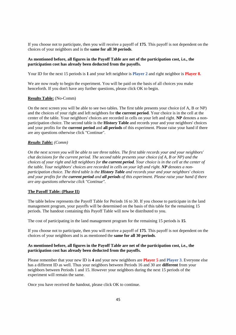
45

If you choose not to participate, then you will receive a payoff of 175. This payoff is not dependent on the choices of your neighbors and is the same for all 30 periods. As mentioned before, all figures in the Payoff Table are net of the participation cost, i.e., the participation cost has already been deducted from the payoffs. Your ID for the next 15 periods is 1 and your left neighbor is Player 2 and right neighbor is Player 8. We are now ready to begin the experiment. You will be paid on the basis of all choices you make henceforth. If you don't have any further questions, please click OK to begin. Results Table: (No-Comm) On the next screen you will be able to see two tables. The first table presents your choice (of A, B or NP) and the choices of your right and left neighbors for the current period. Your choice is in the cell at the center of the table. Your neighbors' choices are recorded in cells on your left and right. NP denotes a non-participation choice. The second table is the History Table and records your and your neighbors' choices and your profits for the current period and all periods of this experiment. Please raise your hand if there are any questions otherwise click "Continue". Results Table: (Comm) On the next screen you will be able to see three tables. The first table records your and your neighbors' chat decisions for the current period. The second table presents your choice (of A, B or NP) and the choices of your right and left neighbors for the current period. Your choice is in the cell at the center of the table. Your neighbors' choices are recorded in cells on your left and right. NP denotes a non-participation choice. The third table is the History Table and records your and your neighbors' choices and your profits for the current period and all periods of this experiment. Please raise your hand if there are any questions otherwise click "Continue". The Payoff Table: (Phase II) The table below represents the Payoff Table for Periods 16 to 30. If you choose to participate in the land management program, your payoffs will be determined on the basis of this table for the remaining 15 periods. The handout containing this Payoff Table will now be distributed to you. The cost of participating in the land management program for the remaining 15 periods is 15. If you choose not to participate, then you will receive a payoff of 175. This payoff is not dependent on the choices of your neighbors and is as mentioned the same for all 30 periods. As mentioned before, all figures in the Payoff Table are net of the participation cost, i.e., the participation cost has already been deducted from the payoffs. Please remember that your new ID is 4 and your new neighbors are Player 5 and Player 3. Everyone else has a different ID as well. Thus your neighbors between Periods 16 and 30 are different from your neighbors between Periods 1 and 15. However your neighbors during the next 15 periods of the experiment will remain the same. Once you have received the handout, please click OK to continue.

46

Appendix B.III: Experimental Handout for High Cost Treatment

Circular Grid with Your Location ID Number:

Payoff from Non-Participation (NP): 175

Cost of Participating in Land Management Program: 40

Payoff Table

Actions Chosen by Neighbors

Your Action Both

Participate Choose A

Both Participate

and one Chooses A & other B

Both Participate and Choose

B

Only one Participates & Chooses A

Only one Participates & Chooses B

No Neighbor Participates

A 210 125 40 125 40 40 B 145 155 165 145 155 145

NP (Non-Participation)

175 175 175 175 175 175

All payoffs are net of participation costs

You

Your Left or Clockwise Neighbor

Your Right OR Anti-clockwise Neighbor