transfer function and linearization - roma tor...
TRANSCRIPT
Transfer functionLinearization
Transfer function and linearization
Daniele Carnevale
Dipartimento di Ing. Civile ed Ing. Informatica (DICII),
University of Rome “Tor Vergata”
Corso di Controlli Automatici, A.A. 2014-2015
Testo del corso: Fondamenti di Controlli Automatici,
P. Bolzern, R. Scattolini, N. Schiavoni.
1 / 13

Transfer functionLinearization
Example
Space state and transfer function
Consider Single Input Single Output (SISO) Linear Time-invariant System(LTI) described by the differential equation (continuous time)
x = Ax+Bu, y = Cx+Du, (1)
with x ∈ Rn, u ∈ R, y ∈ R.The solution ϕ(t, x0, u(·)) := x(t) of (1) with initial condition x0 is
x(t) = eAx0 +
∫ t
0
eA(t−τ)Bu(τ)d τ, [proof: substitute in (1)] (2)
the system output is then
y(t) = CeAx0︸ ︷︷ ︸free response
+C
∫ t
0
eA(t−τ)Bu(τ)d τ +Du(t)︸ ︷︷ ︸forced response
. (3)
The free response is characterized by system modes of the type eλi tthi/hi!,where λi ∈ σ{A} ⊂ C and 0 ≤ hi ≤ n is the dimension of the largest Jordanblock associated to λi. The forced response contains the modes of the inputand the output eαj ttqj/qj !. There might be higher order (tqj+1) polynomialsin the response if αj = λi for some i and j (resonance).
2 / 13
Transfer functionLinearization
Example
Laplace transform: the transfer function
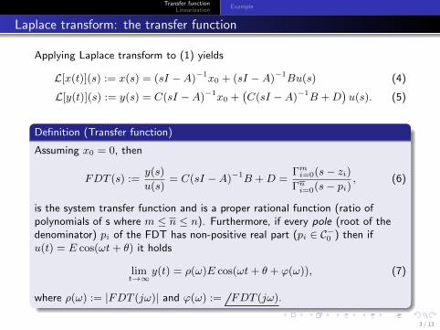
Applying Laplace transform to (1) yields
L[x(t)](s) := x(s) = (sI −A)−1x0 + (sI −A)−1Bu(s) (4)
L[y(t)](s) := y(s) = C(sI −A)−1x0 +(C(sI −A)−1B +D
)u(s). (5)
Definition (Transfer function)
Assuming x0 = 0, then
FDT (s) :=y(s)
u(s)= C(sI −A)−1B +D =
Γmi=0(s− zi)Γni=0(s− pi)
, (6)
is the system transfer function and is a proper rational function (ratio ofpolynomials of s where m ≤ n ≤ n). Furthermore, if every pole (root of thedenominator) pi of the FDT has non-positive real part (pi ∈ C−0 ) then ifu(t) = E cos(ωt+ θ) it holds
limt→∞
y(t) = ρ(ω)E cos(ωt+ θ + ϕ(ω)), (7)
where ρ(ω) := |FDT (jω)| and ϕ(ω) := FDT (jω).
3 / 13
Transfer functionLinearization
Example
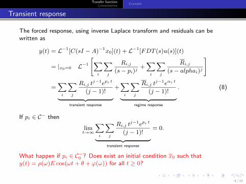
Transient response
The forced response, using inverse Laplace transform and residuals can bewritten as
y(t) = L−1[C(sI −A)−1x0](t) + L−1[FDT (s)u(s)](t)
= |x0=0 L−1
[∑i
∑j
Ri,j(s− pi)j
+∑i
∑j
Ri,j(s− alphai)j
]
=∑i
∑j
Ri,j tj−1epi t
(j − 1)!︸ ︷︷ ︸transient response
+∑i
∑j
Ri,j tj−1eαi t
(j − 1)!︸ ︷︷ ︸regime response
. (8)
If pi ∈ C− then
limt→∞
∑i
∑j
Ri,j tj−1epi t
(j − 1)!︸ ︷︷ ︸transient response
= 0.
What happen if pi ∈ C−0 ? Does exist an initial condition x0 such thaty(t) = ρ(ω)E cos(ωt+ θ + ϕ(ω)) for all t ≥ 0?
4 / 13

Transfer functionLinearization
Example
First order rational functions (not all of them are proper transfer functions)
P1(s) =1
s+ 10, P2(s) =
s+ 10
1, P3(s) =
1
0.1s+ 1, P4(s) =
−0.1s+ 1
1,
P5(s) =1
s− 10, P6(s) =
s+ 100
s+ 10, P7(s) = 2
s+ 10
s+ 100.
−100
−50
0
50
100
Mag
nitu
de (d
B)
10−1 100 101 102 103 104−180
−90
0
90
180
270
360
Phas
e (d
eg)
Bode Diagram
Frequency (rad/s)
P1P2P3P4P5P6P7
Figure: Bode plots - first order functions. 5 / 13
Transfer functionLinearization
Example
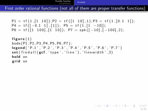
First order rational functions (not all of them are proper transfer functions)
P1 = t f ( 1 , [ 1 1 0 ] ) ; P2 = t f ( [ 1 1 0 ] , 1 ) ; P3 = t f ( 1 , [ 0 . 1 1 ] ) ;P4 = t f ( [−0.1 1 ] , [ 1 ] ) ; P5 = t f ( 1 , [ 1 −10]) ;P6 = t f ( [ 1 1 0 0 ] , [ 1 1 0 ] ) ; P7 = zpk ( [ −1 0 ] , [ −1 0 0 ] , 2 ) ;
f i g u r e ( 1 )bode ( P1 , P2 , P3 , P4 , P5 , P6 , P7 ) ;legend ( ’ P 1 ’ , ’ P 2 ’ , ’ P 3 ’ , ’ P 4 ’ , ’ P 5 ’ , ’ P 6 ’ , ’ P 7 ’ )set ( f i n d a l l ( gcf , ’ t y p e ’ , ’ l i n e ’ ) , ’ l i n e w i d t h ’ , 3 )hold ong r i d on
6 / 13
Transfer functionLinearization
Example
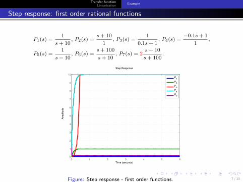
Step response: first order rational functions
P1(s) =1
s+ 10, P2(s) =
s+ 10
1, P3(s) =
1
0.1s+ 1, P4(s) =
−0.1s+ 1
1,
P5(s) =1
s− 10, P6(s) =
s+ 100
s+ 10, P7(s) = 2
s+ 10
s+ 100.
0 1 2 3 4 5 60
1
2
3
4
5
6
7
8
9
10
Step Response
Time (seconds)
Ampl
itude
P1P3P5P6P7
Figure: Step response - first order functions. 7 / 13

Transfer functionLinearization
Example
Step response: first order rational functions
P1(s) =1
s+ 10, P2(s) =
s+ 10
1, P3(s) =
1
0.1s+ 1, P4(s) =
−0.1s+ 1
1,
P5(s) =1
s− 10, P6(s) =
s+ 100
s+ 10, P7(s) = 2
s+ 10
s+ 100.
0 0.2 0.4 0.6 0.8 1 1.2 1.4 1.6 1.8 2−10
−8
−6
−4
−2
0
2
4
6
8
10
time [s ]
y(t)
P1P3P5P6P7
0.51 0.52 0.53 0.54 0.55 0.56 0.57 0.58
−3
−2
−1
0
1
2
3
time [s ]
y(t)
P1P3P5P6P7
Figure: Input response : u(t) = 2 sin(t · 2π · 30). 8 / 13

Transfer functionLinearization
Example
First order rational functions (not all of them are proper transfer functions)
n i = 3 0 ;omega = 2∗ p i ∗ n i ;mytime = 0 : 0 . 0 0 1 : 2 ;u = 2∗ s i n ( omega∗mytime ) ;l i s t a C o l o r i = { ’ r ’ , ’ b ’ , ’ g ’ , ’ k ’ , ’ c ’ , ’ y ’ , ’m’ , ’ r−− ’ , . . .
’ b−− ’ , ’ g−− ’ , ’ k−− ’ , ’ c−− ’ , ’ y−− ’ , ’m−− ’ , ’ r : ’ , ’ b : ’ , ’ g : ’ , . . .’ k : ’ , ’ c : ’ , ’ y : ’ , ’m: ’ , ’ r .− ’ , ’ b.− ’ , ’ g.− ’ , ’ k.− ’ , ’ c .− ’ , . . .’ y .− ’ , ’m.− ’ , ’ r−o ’ , ’ b−o ’ , ’ g−o ’ , ’ k−o ’ , ’ c−o ’ , ’ y−o ’ , ’m−o ’ , . . .’ r−x ’ , ’ b−x ’ , ’ g−x ’ , ’ k−x ’ , ’ c−x ’ , ’ y−x ’ , ’m−x ’ } ;
myFontSize = 1 6 ;
f i g u r e ( 1 )f o r i = 1 : 7
i f ( i ˜= 2 && i ˜= 4) %not p rope r t r a n s f e r f u n c t i o ne va l ( [ ’ y = l s i m (P ’ num2str ( i ) ’ , u , mytime ) ; ’ ] ) ;p l o t ( mytime , y , c e l l 2 m a t ( l i s t a C o l o r i ( i ) ) , ’ L ineWidth ’ , 2 ) ;ho ld ony l i m ([−10 1 0 ] )
endendho ld o f fl egend ( ’ P 1 ’ , ’ P 3 ’ , ’ P 5 ’ , ’ P 6 ’ , ’ P 7 ’ , ’ L o c a t i o n ’ , ’ NorthWest ’ )x l a b e l ( ’ t ime [ s ] ’ , ’ F o n t S i z e ’ , myFontSize , ’ I n t e r p r e t e r ’ , ’ Latex ’ )y l a b e l ( ’ y ( t ) ’ , ’ F o n t S i z e ’ , myFontSize , ’ I n t e r p r e t e r ’ , ’ Latex ’ )ho ld ong r i d on 9 / 13

Transfer functionLinearization
Example
Second order rational functions
P1(s) =ω2n
s2 + 2ζωns+ ω2n
,
P2(s) =1 + 2s
s2 + 1s+ 1, P3(s) =
1−2ss2 + 1s+ 1
,
−100
−50
0
50
100
150
Mag
nitu
de (d
B)
10−2 10−1 100 101 102−180
−135
−90
−45
0
Phas
e (d
eg)
Bode Diagram
Frequency (rad/s)
−40
−30
−20
−10
0
10
Mag
nitu
de (d
B)
10−2 10−1 100 101 102−90
0
90
180
270
360
Phas
e (d
eg)
Bode Diagram
Frequency (rad/s)
P2P3
Figure: Left: P1(s) with ζ ∈ [0, 1]. Right: P2(s) and P3(s). 10 / 13

Transfer functionLinearization
Example
Second order rational functions
P1(s) =ω2n
s2 + 2ζωns+ ω2n
,
P2(s) =1 + 2s
s2 + 1s+ 1, P3(s) =
1−2ss2 + 1s+ 1
, [Non-minum phase plant]
0 5 10 150
0.2
0.4
0.6
0.8
1
1.2
1.4
1.6
1.8
2
time [s ]
y(t)
0 5 10 15−1
−0.5
0
0.5
1
1.5
2
time [s ]
y(t)
Figure: Step response of P1(s) with ζ ∈ [0, 1]. Right: step response of P2(s) (RED)and P3(s) (BLUE).
11 / 13

Transfer functionLinearization
Linearization
Consider the nonlinear differential equation
x = f(x, u, d),
where the system state is x ∈ Rn with input u ∈ Rp and disturbance d ∈ Rq.Let (xe, ue, de) be the equilibrium triple such that f(xe, ue, de) = 0, then thelinearization of the system dynamics around such point is
˙x ≈ ∂f(x, u, d)
∂x
∣∣∣∣(xe,ue,de)
x+∂f(x, u, d)
∂u
∣∣∣∣(xe,ue,de)
u+∂f(x, u, d)
∂d
∣∣∣∣(xe,ue,de)
d,
≈ Ax+Bu+Md, (9)
where x = x− xe, u = u− ue and d = d− de.
12 / 13

Transfer functionLinearization
Linearization: cart-pendulum
Figure: Inverted pendulum with cart (Matlab).
13 / 13