transfer in variable - reward hierarchical reinforcement learning hui li march 31, 2006
TRANSCRIPT

Transfer in Variable - Reward Hierarchical Reinforcement
Learning
Hui Li
March 31, 2006
Overview
• Multi-criteria reinforcement learning
• Transfer in variable-reward hierarchical reinforcement learning
• Results
• Conclusions

Multi-criteria reinforcement learning
• Definition
Reinforcement learning is the process by which the agent
learns an approximately optimal policy through trial and
error interactions with the environment.
Agent Policy
Environment
action atreward rtstate st
rt+1
st+1
Reinforcement Learning
s0a0 : r0
Pss’(a)s1
a1 : r1
Pss’(a)s2
a2 : r2
Pss’(a). . .
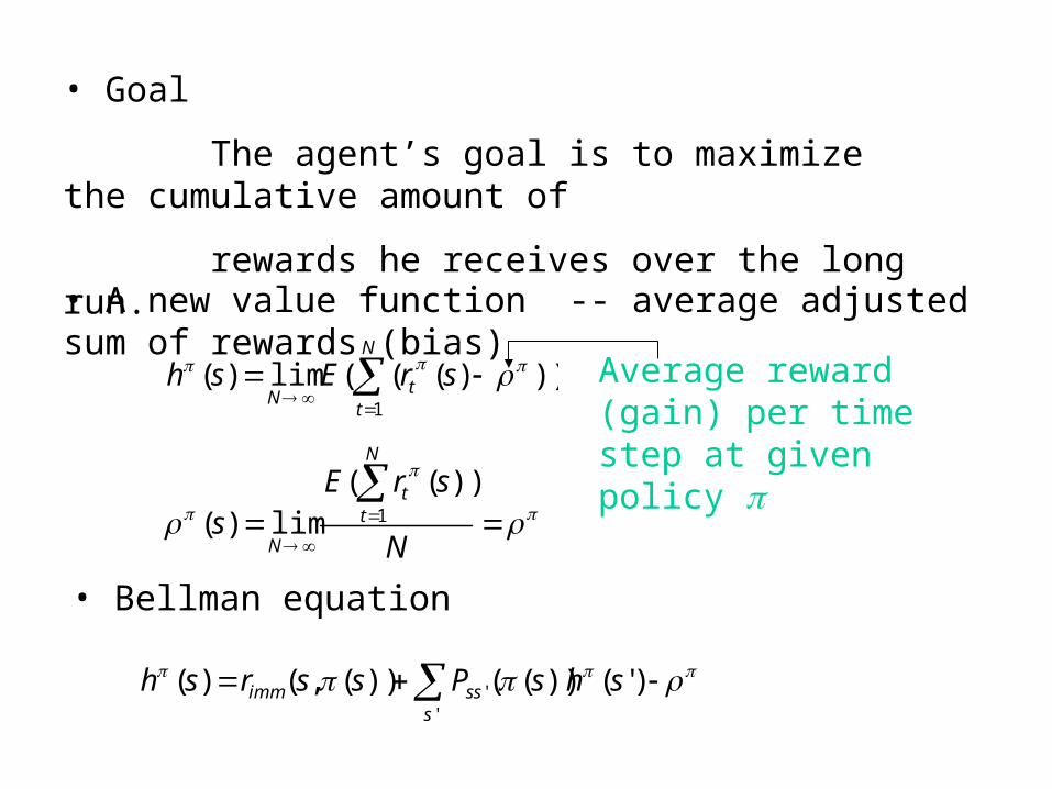
• Goal
The agent’s goal is to maximize the cumulative amount of
rewards he receives over the long run.
• A new value function -- average adjusted sum of rewards (bias)
N
tt
NsrEsh
1
)))(((lim)( Average reward (gain) per time step at given policy
N
srEs
N
tt
N
1
))((lim)(
• Bellman equation
'
' )'())(())(,()(s
ssimm shsPssrsh
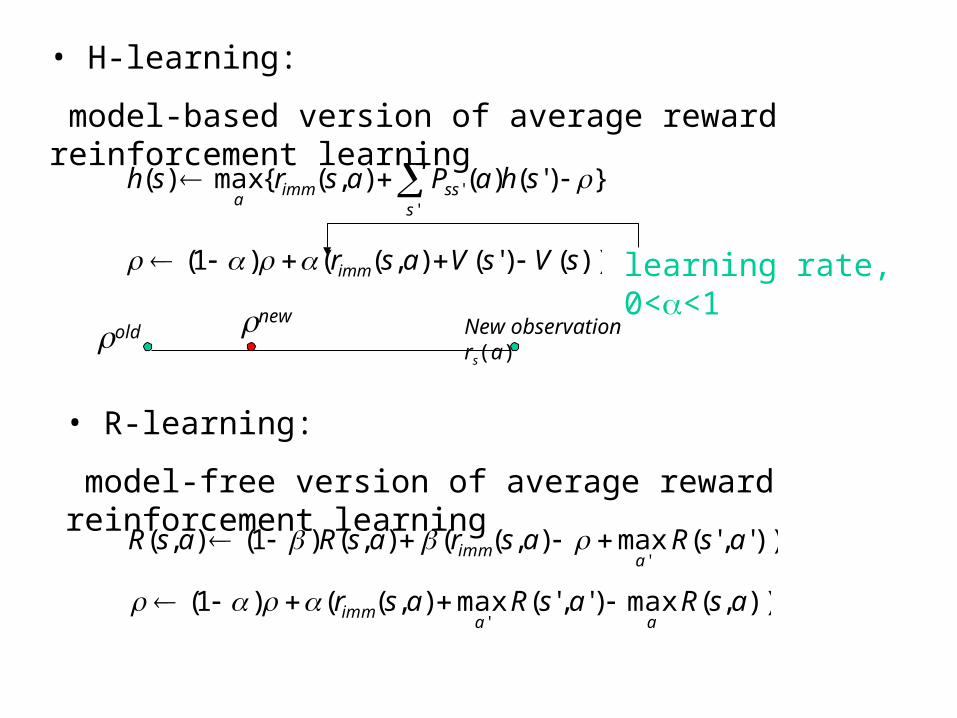
• H-learning:
model-based version of average reward reinforcement learning
})'()(),({max)('
' s
ssimma
shaPasrsh
))()'(),(()1( sVsVasrimm
old new New observation rs(a)
learning rate, 0<<1
• R-learning:
model-free version of average reward reinforcement learning
))','(max),((),()1(),('
asRasrasRasRa
imm
)),(max)','(max),(()1('
asRasRasraa
imm

Multi-criteria reinforcement learning
In many situations, it is nature to express the objective as making some appropriate tradeoffs between different kinds of rewards.
Buridan’s donkey problem
Goals:
• Eating food
• Guarding food
• Minimize the number of steps it walks

Weighted optimization criterion:
i
ii asrwasr ),(),(weight, which represents the importance of each reward
If the weight vector w is static, never changes over time, then the problem reduces to the reinforcement learning with a scalar value of reward.
If the weight vector varies from time to time, learning policy for each weight vector from scratch is very inefficient.

Since the MDP model is a liner transformation, the average reward and the average adjusted reward h(s) are linear in the reward weights for a given policy .
wwi
ii
)()()( shwshwshi
ii
),()(),( asRwsRwasRi
ii

1 2 3
4
5
6
7
• Each line represents the weighted average reward given a policy k ,
wwi
ii
• Solid lines represent those active weighted average rewards
• Dot lines represent those inactive weighted average rewards
• Dark line segments represent the best average rewards for any weight vectors

The key idea:
: the set of all stored policies.
Only those policies which have active average rewards are stored.
Update equations:


Variable-reward hierarchical reinforcement learning
• The original MDP M is split into sub-SMDP {M0,… Mn}, each sub-SMDP representing a sub-task
• Solving the root task M0 solves the entire MDP M
• The task hierarchy is represented as a directed acyclic graph known as the task graph
• A local policy i for the subtask Mi is a mapping from the states to the child tasks of Mi
• A hierarchical policy for the whole task is an assignment of a local policy i to each subtask Mi
• The objective is to learn an optimal policy that optimizes the policy for each subtask assuming that its children’s polices are optimized

GoldminePeasants
Forest
Enemy baseHome base
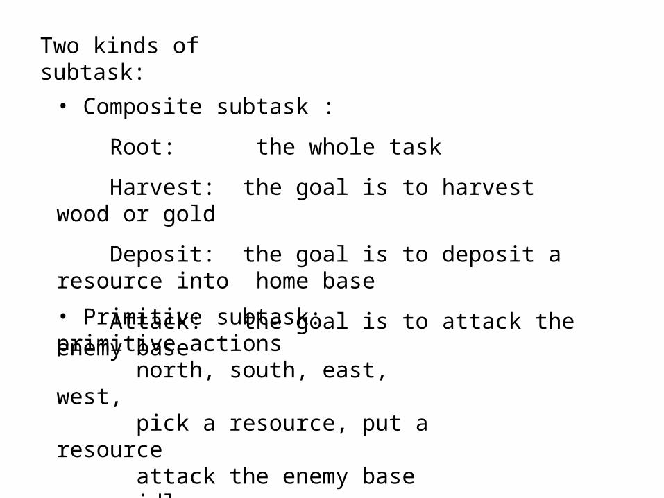
Two kinds of subtask:
• Composite subtask :
Root: the whole task
Harvest: the goal is to harvest wood or gold
Deposit: the goal is to deposit a resource into home base
Attack: the goal is to attack the enemy base
• Primitive subtask: primitive actions north, south, east, west, pick a resource, put a resource attack the enemy base idle

SMDP – semi-MDP
A SMDP is a tuple < S, A, P, r, t >
• S, A, P, r are defined the same as in MDP;
• t(s, a) is the execution tine for taking action a in state s
• Bellman equation of SMDP for average reward learning
)},()'()(),({max)('
' astshaPasrshs
ssimma
A sub-task is a tuple < Bi, Ai , Gi >
• Bi : state abstraction function which maps state s in the original MDP into an abstract state in Mi
• Ai : The set of subtasks that can be called by Mi
• Gi : Termination predicate

The value function decomposition satisfied the following set of Bellman equations:
where
At root, we only store the average adjusted reward

Results• Learning curves for a test reward weight after having seen 0, 1,
2, …, 10 previous training weight vectors
• Negative transfer: learning based on one previous weight is worse than learning from scratch.

Transfer ratio: FY/FY/X
• FY is the area between the learning curve and its optimal value for problem with no prior learning experience on X.
• FY/X is the area between the learning curve and its optimal value for problem given prior training on X.

Conclusions
• This paper showed that hierarchical task structure can
accelerate transfer across variable-reward MDPs more
than in the flat MDP
• This hierarchical task structure facilitates multi-agent
learning

References
[1] T. Dietterich, Hierarchical Reinforcement Learning with the MAXQ Value Function Decomposition. Journal of Artificial Intelligence Research, 9:227–303, 2000.
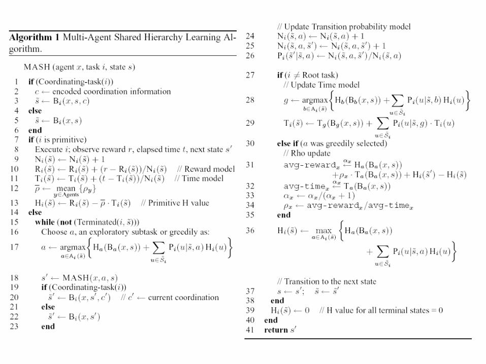
[2] N. Mehta and P. Tadepalli, Multi-Agent Shared Hierarchy Reinforcement Learning. ICML Workshop on Richer Representations in Reinforcement Learning, 2005.
[3] S. Natarajan and P. Tadepalli, Dynamic Preferences in Multi-Criteria Reinforcement Learning, in Proceedings of ICML-05, 2005.
[4] N. Mehta, S. Natarajan, P. Tadepalli and A. Fern, Transfer in Variable-Reward Hierarchical Reinforcement Learning, in NIPS Workshop on transfer learning, 2005.
[5] Barto, A., & Mahadevan, S. (2003). Recent Advances in Hierarchical Reinforcement Learning,
Discrete Event Systems.[6] S. Mahadevan, Average Reward Reinforcement Learning: Foundations, Algorithms, and Empirical Results, Machine Learning, 22, 169-196 (1996)
[7] P. Tadepalli and D. OK, Model-based Average Reward Reinforcement Learning, Artificial intelligence 1998