Transferability of Lidar-derived Basal Area and Stem Density Models within aNorthern Idaho Ecoregion

Patrick A. Feketya�, Michael J. Falkowskib, Andrew T. Hudakc, Theresa B. Jainc, and Jeffrey S. Evansd,e

aDepartment of Forest Resources, University of Minnesota, St. Paul, MN, USA; bDepartment of Ecosystem Science and Sustainability,Colorado State University, Fort Collins, CO, USA; cUnited States Forest Service, Rocky Mountain Research Station, Moscow, ID, USA;dThe Nature Conservancy, Central Science, Fort Collins, CO, USA; eDepartment of Zoology and Physiology, University of Wyoming,Laramie, WY, USA

ABSTRACTA patchwork of disjunct lidar collections is rapidly developing across the USA, often acquiredwith different acquisition goals and parameters and without field data for forest inventory.Airborne lidar and coincident field data have been used to estimate forest attributes acrossindividual lidar extents, where forest measurements are collected using project-specific inven-tory designs. This research explores predicting forest attributes at locations not representedin the training data by combining lidar and field measurements from ecologically similar for-ests. Using field measurements from six lidar units, random forests regression models werecreated by systematically withholding forest inventory data from one lidar unit and using theforest inventory data from the other five units to predict basal area and stem density at thewithheld unit. Results indicate that BA models produce more accurate predictions than stemdensity models when transferred to a lidar unit that did not contain field data. Relative rootmean square errors calculated from the withheld field plots ranged between 32.3%–50.1%for BA and 40.7%–67.3% for stem density models. It is concluded that forest managers mayuse predictive models constructed from ecologically similar forests to obtain a preliminaryestimate of resources, until local field measurement can be obtained.

R�ESUM�EUn ensemble disparate de collections de donn�ees lidar se d�eveloppe rapidement aux �Etats-Unis, souvent acquises avec des objectifs et des param�etres diff�erents et sans donn�ees de ter-rains relatives aux inventaires forestiers. Des donn�ees de terrain concomitantes sont utilis�eespour estimer des attributs forestiers au sein d’�etendues de lidar a�eroport�e individuelles, pourlesquelles les mesures d’int�eret correspondent �a des mod�eles d’inventaires d�etermin�es. Encombinant des mesures de terrain et de lidar provenant de forets �ecologiquement similaires,cette �etude examine la pr�ediction d’attributs forestiers �a des endroits o�u des donn�eesd’entrainement sont absentes. En utilisant des mesures de terrain, des mod�eles de r�egressionproduits par des forets d’arbres d�ecisionnels ont �et�e cr�e�es pour six unit�es de lidar. Un proc�ed�esyst�ematique a �et�e suivi par lequel les donn�ees de chaque unit�e sont retenues et la surfaceterri�ere et densit�e des tiges de cette unit�e sont ensuite estim�es avec les donn�ees des cinqunit�es restantes. Les r�esultats indiquent que les estimations de surface terri�ere sont plusrobustes que pour la densit�e de tiges lorsque les mod�eles sont transf�er�es �a une unit�e de lidarpour laquelle les donn�ees de terrain sont absents. Les erreurs quadratiques moyennes rela-tives calcul�ees pour les �echantillons retenus sont entre 32.3 % et 50.1 % pour les mod�eles desurface terri�ere et entre 40.7 % et 67.3 % pour la densit�e des tiges. Nous concluons que,jusqu’�a ce que des mesures de terrain locales puissent etre acquises, il est possible d’obtenirdes estimations pr�eliminaires de ressources foresti�eres en utilisant des mod�eles pr�edictifs con-struits �a partir d’�echantillons de forets �ecologiquement similaires.

ARTICLE HISTORYReceived 10 November 2017Accepted 13 March 2018

Introduction

Airborne light detection and ranging (lidar) is widelyused in forest management to meet various objectives

(Maltamo et al. 2014) such as predicting timber volume(White et al. 2014), identifying forest structure charac-teristics important for wildlife habitat (Martinuzzi et al.

CONTACT Patrick A. Fekety patrick.fekety@colostate.edu*Current Address: Colorado State University, Department of Ecosystem Science and Sustainability, Fort Collins, CO, 80523, USA

The work of Andrew Hudak and Theresa Jain was authored as part of their official duties as Employees of the United States Government and is therefore a work of the UnitedStates Government. In accordance with 17 USC. 105, no copyright protection is available for such works under US Law.

Patrick Fekety, Michael Falkowski and Jeffrey Evans hereby waive their right to assert copyright, but not their right to be named as co-authors in the article.

CANADIAN JOURNAL OF REMOTE SENSING2018, VOL. 44, NO. 2, 131–143https://doi.org/10.1080/07038992.2018.1461557

2009), and using high resolution lidar-derived digitalterrain models (DTM) to locate forest roads (Arugaet al. 2005). As more lidar data are being acquired, apatchwork of disjunct datasets is developing acrossregional extents. In the United States, contiguouscounty and state-level lidar collections exist, althoughthe motivation for large-scale collections is typically thedevelopment of high-resolution digital terrain models(DTMs), rather than characterizing forest vegetation (e.g.,3DEP 2016; MNGeo 2015). Field measurements describ-ing vegetation are not typically collected when the lidarare acquired for non-forestry related objectives. However,forest managers typically establish inventory plots to pro-vide training data for predictive models when lidar collec-tions are motivated by forest management needs. Toprovide the most benefit, coincident plot-level field dataare collected as temporally close to the lidar acquisition aspossible (White et al. 2013; Eskelson et al. 2009).Although forest type and stand age will affect the abilityto use non-temporally coincident data, field plots meas-ured up to 5 years before the lidar collection have beenused (Zald et al. 2014). Leveraging temporally appropriateinventory measurements and lidar data in ecologicallysimilar areas may facilitate the prediction of forest inven-tory attributes to lidar collections that contain little or nolocal forest inventory measurements, thus transferring anexisting predictive model to a new spatial location.

Managers need up-to-date information characteriz-ing forest resources, such as basal area and stem dens-ity, to support both operational and long-termplanning. Predictive modeling using lidar can provideresource estimates across large spatial extents (Næsset2004) while repeat lidar collections allow the character-ization of resource change (Hudak et al. 2012). Lidardata, in conjunction with coincident field data, havebeen used in predictive modeling of forest inventoryattributes with success (e.g., Næsset 2002; R2 0.80–0.93for volume). Several studies have predicted forestattributes solely from disjunct lidar collections (Lefskyet al. 2002; Hudak et al. 2006; Næsset 2007). Forexample, Næsset (2007) constructed linear regressionmodels to predict six forest inventory metrics by com-bining two lidar acquisitions, with similar collectionparameters, that were 50 km apart in Norway andachieved excellent results (e.g., R2 for volume rangedbetween 84% and 89%). Across a larger spatial extent,Lefsky et al. (2002) built a regression model to predictaboveground biomass across three North Americanbiomes and achieved an R2 of 0.84. Using full wave-form lidar data and aerial imagery, Latifi and Koch(2012) created imputation models to predict forestattributes using various combinations of local andnon-local data. They found that models built

exclusively from non-local data resulted in the largestrelative errors, but adding a portion of the withhelddata substantially decreased the error. While the previ-ous studies discussed spatially transferring models,Fekety et al. (2015) demonstrated the feasibility oftemporally transferring lidar-based basal area imput-ation models and achieved satisfactory results (e.g.,R2¼ 0.78–0.79). Combining spatially and temporallydisjunct lidar data in a statistical modeling frameworkcould allow for the creation of prediction models toestimate forest inventory data to newly acquired lidarcollections, ultimately providing a first pass estimate offorest resources.

The overarching goal of this research is to createpredictive models by combining spatially and tempor-ally disjunct lidar and field data and evaluating per-formance when the model is transferred to locationswhere lidar data exist, but do not have ground truthmeasurements. We hypothesized transferring models tounsampled, yet ecologically similar, forests will producepredictions that are statistically equivalent to groundtruthed values. To achieve this goal, we leverage a data-base consisting of six independently collected fielddatasets and six spatially and temporally disjunct lidarcollections throughout northern Idaho. A series ofmodels were created by systematically withholding fielddata from one lidar unit and treating the withheld dataas a validation dataset. This procedure may provideresource managers with acceptable estimates of forestattributes at locations that do not have local field data.

Methods and materials

Study area

The study area for this project is the InlandNorthwest region of the Northern Rocky Mountainecoregion (Figure 1). Forests in the Inland Northwestare mixed conifer with Douglas-fir (Pseudotsuga men-ziesii (Mirb.) Franco), grand fir (Abies grandis(Douglas ex D. Don) Lindl.), western redcedar (Thujaplicata Donn ex D. Don), and western hemlock(Tsuga heterophylla (Raf.) Sarg.) as the primary climaxspecies (Cooper et al. 1991). The region is occupiedby primarily north–south mountain ranges separatedby intermontane valleys (Taylor 2012). The study areaencompasses elevations between 650 m and 2000 m(mean 1090m) and slopes up to 65% (mean 33%).Geology is a mixture of the sedimentary BeltSupergroup and Idaho Batholith granitics (Cooperet al. 1991); local ash caps deposited by the MountMazama eruption (c.5700 BCE) created localized pock-ets of highly productive forests (Kimsey et al. 2008).

132 P. A. FEKETY ET AL.

Climate is moderated by the maritime influences ofthe Pacific Ocean. Precipitation is greater at higherelevations, caused by orographic lifting, with themajority of precipitation occurring in the winter.

This study focuses on six locations distributedthroughout northern Idaho that have associated fieldand lidar measurements. Priest River ExperimentalForest (PREF) is a 2,758 ha forest managed by theU.S. Forest Service, Rocky Mountain Research Station,located approximately 18 km north of Priest River, IDand noted for its diverse mixed conifer forest. The12,948 ha Fernan lidar extent covers the Fernan, BlueCreek, and Wolf Lodge watersheds, which drain intothe north end of Lake Coeur d’Alene. Sixty-six per-cent of the Fernan extent is private land consisting ofprivate industrial forest, agricultural, and wildlandurban interface, while the remaining 34% is publicforest primarily managed by the U.S. Forest Service aspart of the Coeur d’Alene Ranger District of theIdaho Panhandle National Forests. The Tepee Potterlidar unit covers 11,737 ha and is also managed by theIdaho Panhandle National Forests and is 39 km eastof Coeur d’Alene, ID. The Moscow Mountain

19,889ha study area located 18 km from Moscow, ID isprimarily private industrial forests (43%) with inhold-ings of private non-industrial forests (39%) and statelands (18%). The St. Joe project area (Figure 1) is55,723ha managed mainly by private timber companies(62%) and the Idaho Panhandle National Forests(38%). The 10,864 ha area referred to as Upper Lolo ismanaged by the Nez Perce-Clearwater National Forestsand is located 38 km northwest of Kooskia, ID.

Field plot data

Six independent field data collection exercises were per-formed within the six lidar extents and sampling con-cluded within a year of the respective lidar collection.The field data were collected for various reasons andtherefore differ in sampling design and data collectionprotocols. At a minimum, all study designs called for acomplete inventory of live and standing dead trees witha diameter breast height (DBH) greater than 12.7 cm tobe measured within the plots. Measurement protocolsfor smaller trees varied among inventory designs andwere excluded from these analyses. All field plots weregeolocated with a Trimble (Sunnyvale, CA, USA) globalnavigation satellite system (GNSS) and differentiallycorrected using local base stations. In total, 360 fieldplots throughout the Inland Northwest were used inthis study (Table 1). Field plot locations were locatedfollowing stratified random designs, which were specificto each data collection exercise. The landscape stratifi-cation for field plots located on the Coeur d’AleneRiver District (herein referred to as CdA) data requirefurther explanation because the stratified randomdesign considered both the Fernan and Tepee Potterlidar units. Consequently, for this study, the field meas-urements were separated into two datasets based ontheir coincident lidar unit; CdA-East plots (n¼ 24)were located in the Tepee Potter lidar unit while theCdA-West plots (n¼ 10) were located in the Fernanlidar unit. The CdA-East plots were combined with theTepee Potter plots for model construction.

Table 1. Field data collection parameters.Field dataset n Year Lidar unit Plot Area (m2) Plot design Sampling design

CdA-East 24 2015 Tepee Potter 400 Fixed radius Stratified by elevation, transformed aspect, and wetnessCdA-West 10 2015 Fernan 400 Fixed radius Stratified by elevation, transformed aspect, and wetnessMoscow Mtn. 85 2009 Moscow Mtn. 400 Fixed radius Stratified by elevation, solar insolation, and NDVIcPREF 96 2011 PREF 400 Fixed radius Stratified by forest type and canopy coverSt. Joe 79 2003-2004 St. Joe 400 Fixed radius Stratified by elevation and solar insolationTepee Potter 39 2014 Tepee Potter 400 Fixed radius Stratified by elevation, solar insolation, and NDVIUpper Lolo 27 2007 Upper Lolo Creek 400 Fixed radius Stratified by elevation, transformed aspect, and NDVIc

Note: CDA-East and CDA-West were part of the same data collection exercise. Both Tepee Potter and Fernan lidar units were combined for thestratification.

NDVI: Normalized difference vegetation index.NDVIc: Normalized difference vegetation index corrected by middle infrared.

Figure 1. Location of project areas within Inland Northwest.

CANADIAN JOURNAL OF REMOTE SENSING 133

Response variables

The response variables predicted were BA and stemdensity, which are valuable for regional scale forestmanagement and planning. Summary statistics for theresponse variables are found in Table 2.

Explanatory variables

Data from six independent, discrete-return, airbornelidar collections located within the Inland Northwestof northern Idaho, USA were used for this study(Figure 1). Lidar were collected with Leica lidar scan-ners; however, differences in acquisition parametersvaried considerably between some of the acquisitions,largely resulting from lidar sensor improvementsacross the 12-year time period considered in thisstudy (Table 3). All of the lidar datasets were collectedin snow-free conditions, which can limit the windowof lidar collections, especially at higher elevationswithin the study area. With the exception of westernlarch (Larix occidentalis), the major tree species in thestudy area are evergreen, and consequently in apersistent leaf-on state. The Fernan lidar data werecollected while deciduous understory shrubs were inleaf-off conditions.

When available, the vendor-identified groundreturns were accepted as accurately classified. Fernanand Tepee Potter ground returns were identified bythe vendor using TerraScan V.15 (Terrasolid Ltd,Helsinki, Finland). Ground returns within the PREFlidar extent were classified with Lidar FeatureExtraction – the vendor’s proprietary classificationalgorithm. The lidar vendor did not classify groundreturns for the Moscow Mountain, St. Joe and UpperLolo lidar collections; therefore, ground returns wereidentified using the multi-scale curvature classification(MCC)-lidar algorithm (Evans and Hudak 2007),which fits a multi-scale thin plate spline model toclassify lidar ground returns. A 1-m DTM was gener-ated from the classified ground returns using FUSIONv3.60 (McGaughey 2016) for the Fernan, MoscowMountain, PREF, Tepee Potter, and Upper Lolo lidarcollections. The lidar pulse density at St. Joe wasinsufficient to generate a 1-m DTM (Table 3); there-fore, a 2-m DTM was generated. Figure 2 shows aconceptual model describing the lidar processing andmodel building processes.

Lidar returns that fell within the field plots wereextracted using FUSION (McGaughey 2016) andheight-normalized point clouds were generated viaDTM subtraction. Following the results of Næsset

Table 3. Lidar collection parameters.Lidar Collection Fernan Moscow Mountain PREF St. Joe Tepee Potter Upper Lolo

Date collected Dec 2014 & Feb 2015 Jun 2009 July 2011 Summer 2003 May 2015 Sept–Oct 2006Vendor QSI Environmental Watershed

Sciences, IncWatershed

Sciences, IncHorizons, Inc. QSI Environmental Watershed

Sciences, Inc.Sensor Leica ALS 70 and

ALS 80Leica ALS50 Phase II Leica ALS50 Phase II Leica ALS40 Leica ALS 70 Leica ALS50 Phase II

Pulse frequency 195 kHza N/A 73.5 kHz 20 kHz 180 kHza 83 kHzScan angle þ/– 15 degrees þ/– 14 degrees þ/– 15 degrees þ/– 15 degrees þ/– 15 degrees þ/– 14 degreesAltitude 1,400 m AGL 2,000 m AGL 1,500 m AGL 2,438 m AGL 1,450 m AGL 1,100 m AGLSpatial extent 12,948 ha 19,889 ha 4,041 ha 55,723 ha 11,737 ha 10,864 haWavelength 1,064 nm 1,064 nm 1,064 nm 1,064 nm 1,064 nm 1,064 nmVertical accuracy 3.4 cm 4.3 cm 4.9 cm N/A 5.8 cm 6.3 cmPulse density 16.4 pulses/m2 8.5 pulses/m2 10.4 pulses/m2 0.6 pulses/m2 20.8 pulses/m2 4.7 pulses/m2

Footprint 31 cm 30–45 cm 34 cm 30 cm 32 cm 24 cm

Note: AGL: above ground level.N/A: not available.aOperating "Single Pulse in Air" mode.

Table 2. Summary of plot-level basal area and stand density estimates.Basal area (m2/ha) Stem sensity (stems/ha)

Project Total plots Treeless plots Min Mean Median Max SD Min Mean Median Max SD

CdA-East 24 3 0 34 32 88 21 0 403 436 872 252CdA-West 10 1 0 20 19 49 15 0 229 212 598 195Moscow Mountain 85 6 0 25 21 109 21 0 358 299 1122 285PREF 96 9 0 31 27 99 24 0 387 349 1645 320St. Joe 79 1 0 37 37 112 24 0 543 449 1570 348Tepee Potter 39 1 0 30 32 93 18 0 403 449 872 229Upper Lolo 27 6 0 35 36 92 26 0 300 324 623 208All projects 360 27 0 31 29 112 23 0 406 374 1645 304

Note: CdA-East and CdA-West were collected during a single campaign. Both Fernan and Tepee Potter lidar collections were combined for thisstratification.

134 P. A. FEKETY ET AL.

(2009) and Bater et al. (2011), plot-level point cloudsconsisting of only first returns were processed withFUSION to calculate plot-level height, strata, andcover metrics. A 1.37 m (equivalent to breast height)cutoff was used when calculating lidar height andcover metrics.

Topographic metrics influence forest productivity(Stage and Salas 2007), and thus stand conditions.FUSION was used to create gridded rasters of eleva-tion, slope, and aspect, which were inputted toGeographic Resources Analysis Support System v7.2.0(GRASS Development Team 2017) to create additionaltopographic metrics. A full list of predictor variablescan be found in Table 4.

Model specification: random forests regression

Random forests (Breiman 2001) regression modelswere created using the randomForest package (Liawand Wiener 2002) in R statistical software (R CoreTeam 2017) to predict BA and stem density.Numerous papers describe the random forests algo-rithm applied in a natural resource context (e.g.Prasad et al. 2006; Lawrence et al. 2006; Cutler et al.2007). Six BA and six stem-density prediction models

Figure 2. Conceptual model describing major steps of the lidar processing and model building.

Table 4. Potential explanatory variables.Description of explanatory variables Data source

H05Pct: Height 5th percentile FUSIONH25Pct: Height 25th percentile FUSIONH50Pct: Height 50th percentile FUSIONH75Pct: Height 75th percentile FUSIONH95Pct: Height 95th percentile FUSIONHmean: Height mean FUSIONHstdv: Height standard deviation FUSIONHskew: Height skewness FUSIONHkurt: Height kurtosis FUSIONCRR: Canopy relief ratio (McGaughey 2016) FUSIONStratum 0: Percentage lidar returns <0.15 m FUSIONStratum 1: Percentage lidar returns >0.15 m and

<1.37 mFUSION

Stratum 2: Percentage lidar returns >1.37 m and<5.0 m

FUSION

Stratum 3: Percentage lidar returns >5 m and <10 m FUSIONStratum 4: Percentage lidar returns >10 m and <20 m FUSIONStratum 5: Percentage lidar of returns >20 m and �0 m FUSIONStratum 6: Percentage lidar of returns >30 m FUSIONPct1Rtn_1.37: Percentage lidar first returns above 1.37 m FUSIONPct1Rtn_mean: Percentage lidar first returns above

height meanFUSION

Elev: DTM elevation at 20 m resolution FUSIONSlope: Percent slope at 20 m resolution FUSIONTrAsp: Transformed aspect at 20 m resolution Calculated in RSCOSA: Slope cosine aspect transformation Calculated in RSSINA: Slope sine aspect transformation Calculated in RGlobRadEquinox: Radiance estimate on 23 Sept GRASSaccumulation: Hydrologic flow accumulation GRASStci: Topographic convergence index GRASStwi: Topographic wetness index GRASS

CANADIAN JOURNAL OF REMOTE SENSING 135

were created by systematically withholding the refer-ence observations that were located in one of the sixlidar units. The resulting models are used to evaluatehow well a given model could be expected to performwhen transferred to a new lidar unit (represented bythe withheld area). In this study the models are desig-nated by the name of the lidar unit to which they willbe transferred. For example, the Fernan models areused to predict BA and stem density at sites locatedin the Fernan lidar unit and trained using field andlidar data collected in the Moscow Mountain, PREF,St. Joe, Tepee Potter, and Upper Lolo lidar units.

Model selection process

We expected many of the potential explanatory varia-bles to be highly correlated (Spearman rank correl-ation coefficient >0.85), and it was anticipated thatsome lidar metrics would also exhibit multi-collinear-ity; therefore, the rfUtilities R library was used to per-form a Gram-Schmidt QR-decomposition to identifyand remove multi-collinear variables (Evans andMurphy 2017; Falkowski et al. 2009). Multi-collinearvariables were identified and removed before con-structing each model.

A model selection tool centered on the random for-ests algorithm (Breiman 2001) was used in the modelselection processes. Model selection was performedusing the rf.modSel function from the rfUtilities pack-age to select the best suite of predictor variables foreach response variable (Murphy et al. 2010). Throughan iterative process, the function builds a random for-ests model consisting of all potential predictor varia-bles and subsequently builds additional models byeliminating the potential predictor variable with thelowest model improvement ratio (MIR). The processis repeated until the model error does not change or asingle variable remains. The selected parameters areassociated with the model exhibiting the greatest per-centage variation explained and the least squared-error. The results from the rfUtilities model selectionprocess were used to specify the models. In all cases,the model selection tool was run 100 times for eachresponse variable to investigate the stability in theselected model.

Model evaluation

The predictive models were evaluated with bothinternal fit statistics and performance statistics. Therandom forests models fit statistics were calculatedwith the rf.crossValidation function from rfUtilities

(Evans and Murphy 2017). Cross-validated estimatesof root-mean-square error (RMSE; Equation 1) werecalculated between the observed and predicted valuesusing the training data. RMSE was normalized by themean observation to allow for comparisons amongthe models (Equation 2).

RMSE ¼ffiffiffiffiffiffiffiffiffiffiffiffiffiffiffiffiffiffiffiffiffiffiffiffiffiffiffiffiffiffiffiffiffiffiffiffiffiffiffiffiffiffiffiffiffiffiffiffiffiffiffiffiffiffiffiffiffiffiffiffiffiffiffiffiffiffiffiffi1n

Xpredictions�observationsð Þ2

r[1]

RMSE% ¼ RMSE

mean observationsð Þ �100% [2]

where RMSE% is the normalized RMSE. The medianpercentage variation explained (pseudo-R2) andRMSE% were reported, along with their standarddeviations, for 100 cross-validations.

RMSE% was also reported as a performance statis-tic and was calculated using the withheld data and itscomplementary predictions in order to determine howwell a model would transfer to a new area.

Predictions were further evaluated using statisticalequivalence tests. Standard t-tests were not usedbecause they are designed to test for differences, notsimilarities, between two statistics (Robinson andFroese 2004). Failure to reject the null hypothesis fora standard t-test suggests there is not sufficient evi-dence that two datasets are not equal; however, thisdoes not guarantee that two datasets are similarbecause the statistical power of the chosen test mightbe weak (Robinson and Froese 2004). Statisticalequivalence tests set the null hypothesis such that thedatasets are dissimilar and requires the data to proveotherwise. Generic forms for the hypotheses are:

H0: Model predictions are dissimilar to observedvalues; and

H1: Model predictions are similar (i.e. equivalent)to observed values.

Equivalence tests were performed in R using thebootstrapped implementation from the equivalencepackage (i.e. equiv.boot; Robinson 2016), which usesthe two one-sided test (TOST) of equivalence. TheTOST examines if the intercept (b0) and slope (b1)estimators from the linear regression between themodel predictions and true values are contained in apredetermined region of equivalence. The interceptcomponent of the equivalence test is a measure ofbias, whereas the slope component is a measure ofproportionality (Robinson et al. 2005). In this study,the test of bias determines if the mean of the observa-tions is equivalent to the mean of the predictions; thetest for proportionality determines if the slopebetween model predictions and observations is equiva-lent to one.

136 P. A. FEKETY ET AL.

If the confidence intervals (CI) from the TOSTaround the estimator (i.e., intercept or slope) areentirely contained within the region of equivalencethen there is evidence to reject the null hypothesis,meaning the two data sets are statistically equivalent.The default region of equivalence of ±25% was usedin this study and has been called a conservative regionof equivalence (Wellek 2003; Robinson and Froese2004) and has been used in other studies (e.g.,Falkowski et al. 2008; Penner et al. 2013).Additionally, the exact regions of equivalence werecalculated to determine the smallest region of equiva-lence when the null hypothesis is no longer rejected.A smaller region of equivalence indicates better agree-ment between the observations and predictions. Theregion of equivalence for bias was calculated as a per-centage and in absolute units (i.e., m2/ha or stems/ha). The region of equivalence for proportionality wascalculated only as a percentage because the slope isdimensionless.

Results

Nineteen lidar height metrics and 9 topographic met-rics were considered as potential explanatory variables(Table 4). After removing multi-collinear variables

and performing the model selection process, theexplanatory variables were pared down to a subset ofonly lidar height metrics (Table 5).

BA and stem density random forests predictionmodels were created and subsequently used to predictBA and stem density at the field plots that were with-held from the model training. Cross-validation fit sta-tistics calculated solely from the training data showedbetter fit for the BA models than the stem densitymodels in terms of variance explained and RMSE%(Table 6). When comparing the predictions with with-held observations, RMSE% performance statistics werewithin one standard deviation of the cross-validatedRMSE% fit statistics for 10 out 12 models – UpperLolo BA model and Fernan stand density model per-formance RMSE% were greater than one standarddeviation (Tables 6 and 7).

Equivalence tests show BA predictions for MoscowMountain, PREF, and Tepee Potter were statisticallyequivalent to the measured BA, in terms of both biasand proportionality at a ± 25% region of equivalence(Figure 3A). The 95% CI of the bias component forthe Fernan BA predictions extends outside the lowerregion of equivalence indicating positive biases (i.e.,over-predictions). These over-predictions can also beseen by investigating the scatter plot in Figure 4A,which shows 9 of the 10 Fernan BA predictions werelarger than the observed value. When the 95% CI ofthe bias component extends outside the upper regionof equivalence, such as with the Upper Lolo BApredictions, this indicates that the model is under-predicting the attribute on average (Figure 3A). The95% CI of proportionality component extends outsidethe lower range of region of equivalence for Fernanand Upper Lolo BA predictions, which denotes thatmodel over-predicts low BA plots and under-predictshigh BA plots. Likewise, the 95% CI of proportionalitycomponent extends outside the upper range ofregion of equivalence for St. Joe denoting that model

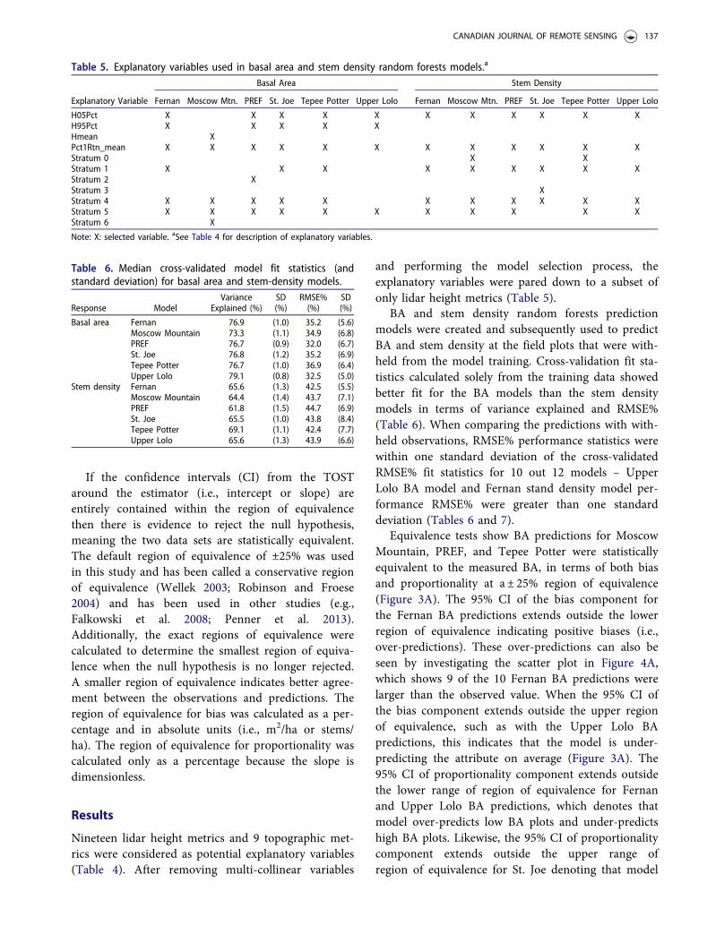
Table 5. Explanatory variables used in basal area and stem density random forests models.a

Basal Area Stem Density

Explanatory Variable Fernan Moscow Mtn. PREF St. Joe Tepee Potter Upper Lolo Fernan Moscow Mtn. PREF St. Joe Tepee Potter Upper Lolo

H05Pct X X X X X X X X X X XH95Pct X X X X XHmean XPct1Rtn_mean X X X X X X X X X X X XStratum 0 X XStratum 1 X X X X X X X X XStratum 2 XStratum 3 XStratum 4 X X X X X X X X X X XStratum 5 X X X X X X X X X X XStratum 6 X

Note: X: selected variable. aSee Table 4 for description of explanatory variables.

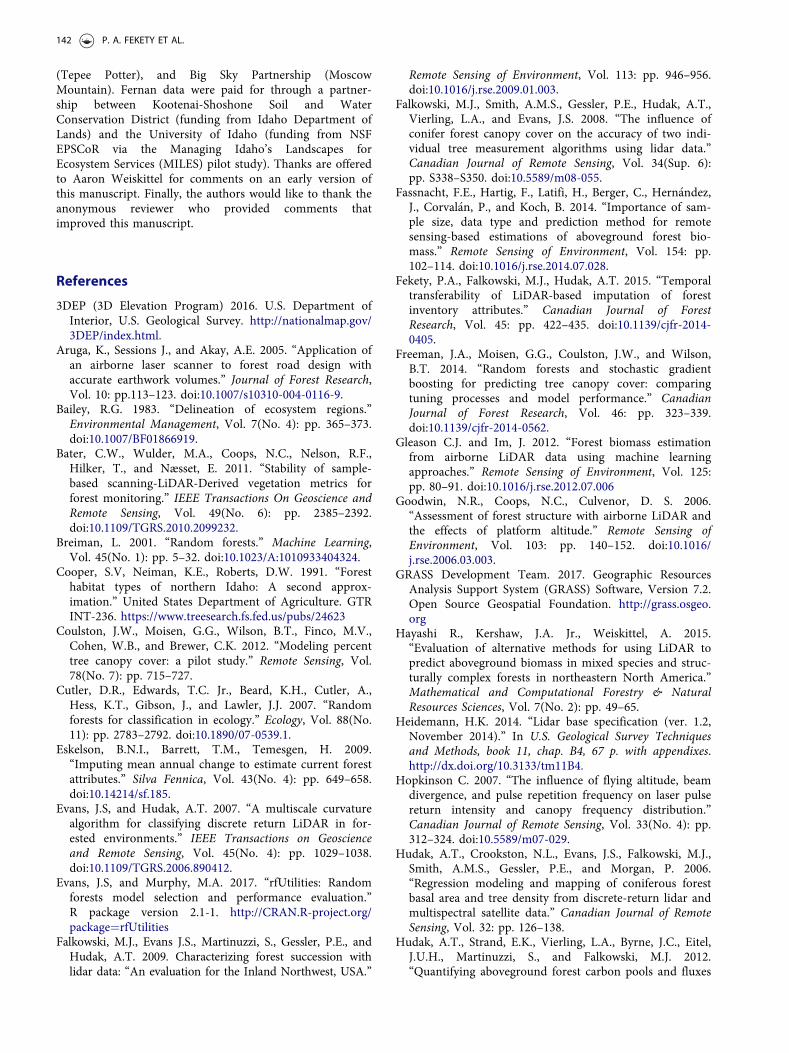
Table 6. Median cross-validated model fit statistics (andstandard deviation) for basal area and stem-density models.

Response ModelVariance

Explained (%)SD(%)

RMSE%(%)

SD(%)

Basal area Fernan 76.9 (1.0) 35.2 (5.6)Moscow Mountain 73.3 (1.1) 34.9 (6.8)PREF 76.7 (0.9) 32.0 (6.7)St. Joe 76.8 (1.2) 35.2 (6.9)Tepee Potter 76.7 (1.0) 36.9 (6.4)Upper Lolo 79.1 (0.8) 32.5 (5.0)

Stem density Fernan 65.6 (1.3) 42.5 (5.5)Moscow Mountain 64.4 (1.4) 43.7 (7.1)PREF 61.8 (1.5) 44.7 (6.9)St. Joe 65.5 (1.0) 43.8 (8.4)Tepee Potter 69.1 (1.1) 42.4 (7.7)Upper Lolo 65.6 (1.3) 43.9 (6.6)

CANADIAN JOURNAL OF REMOTE SENSING 137

under-predicts low BA plots and over-predicts highBA plots. In addition to the predetermined ±25%region of equivalence, the limit at which the equiva-lence test fails was also calculated (Table 7).Graphically, these values indicate the point when the95% CI and region of equivalence share an edge. Aspreviously stated, the Fernan predictions were notequivalent at a ± 25% region of equivalence; Table 7shows the minimum acceptable region of equivalenceas ±26.5% and ±29.7% for slope and proportionality,respectively. The bias region of equivalence can beconverted to absolute units; for example the ±26.5%region of equivalence for the Fernan BA indicates thepredictions are statistically equivalent to the observa-tions if biases of up to ±8.5m2/ha of basal areaare acceptable.

The stem-density models have larger errors com-pared with the BA models (see Table 7) and is alsoseen by the wider dispersion around the 1-to-1 line inFigure 5. Equivalence tests show stem-density predic-tions for Moscow Mountain and PREF were equivalent,

in terms of bias and proportionality, to the measuredstem density (Figure 3B). Moscow Mountain stemdensity was the best performing model as indicated bythe narrowest calculated regions of equivalence (seeTable 7). Fernan, Tepee Potter, and Upper Lolo 95%CI around the proportionality component of theequivalence test extends past the lower region ofequivalence. These models over-predict less densestands and under-predict denser stands. The stem-density predictions for the Fernan model are consider-ably over-predicted as seen by the small proportion ofoverlap between the 95% CI and region of equivalence(Figure 3B) and this is also apparent by investigatingthe scatter plot in Figure 5A.

Discussion

We evaluated the effectiveness of transferring randomforests models to predict forest attributes in areaswhere lidar exist, but forest inventory measurementsdo not. This was achieved by combining several

Table 7. Model performance reported as normalized root-mean-square error (RMSE%) and the region of equivalence limit whenthe equivalence test no longer rejects the null hypothesis.

Basal Area Stem Density

Model n RMSE% (%) R0 (m2/ha) R0 (%) R1 (%) RMSE% (%) R0 (stems/ha) R0 (%) R1 (%)

Fernan 10 33.8 ±8.5 ±26.5 ±29.7 67.3 ±184.2 ±53.1 ±52.2Moscow Mountain 85 35.9 ±2.5 ±7.9 ±12.5 40.7 ±36.0 ±10.4 ±21.1PREF 96 40.0 ±5.5 ±17.1 ±17.9 47.6 ±86.2 ±24.8 ±17.3St. Joe 79 33.4 ±6.8 ±21.3 ±32.6 43.0 ±127.0 ±36.6 ±20.0Tepee Potter 63 32.3 ±2.7 ±8.6 ±20.2 44.4 ±51.5 ±14.8 ±39.7Upper Lolo 27 50.1 ±10.3 ±32.2 ±47.5 48.3 ±100.7 ±29.0 ±48.2

Note: R0: region of equivalence for bias.R1: region of equivalence for proportionality.

Figure 3. Results of bootstrapped equivalence tests for (A) basal area, and (B) stem density. The tests of biases are centered onthe mean observation and the test of proportionality is centered on a slope of one. The shaded polygon represents the region ofequivalence. The black bars represent the 95% confidence interval (CI). The equivalence test is satisfied when the 95% CI is com-pletely contained in the region of equivalence.

138 P. A. FEKETY ET AL.

disjunct lidar and forest inventory datasets into mod-els that predicted BA and stand density and transfer-ring the model to lidar units excluded from thetraining data. Model performance was evaluated bycalculating errors (RMSE%) and equivalence tests. Welearned several lessons surrounding the combinationof disjunct lidar acquisitions and field data for pre-dicting forest inventory data to lidar collections with-out local reference observations. The remainder of thediscussion covers these points in greater detail.

Model specification

Random forests modeling is one of many predictionmethods used in natural resource applications and itwas not our intention to test whether random forestsprovides the best results. Studies have shown that

random forests outperformed (e.g. Coulston et al.2012; Fassnacht et al. 2014), under-performed (e.g.Hayashi et al. 2015; Gleason and Im 2012), or per-formed similarly to (e.g. Freeman et al. 2014) othermodeling techniques. Our intent was to build a parsi-monious model which emulated the process that aresource manager could take to predict forest attributeat locations without field data; other modeling techni-ques could be explored.

Modelling considerations

The extent of a lidar collection is often defined bymanagement boundaries (e.g., PREF) or watershedboundaries (e.g., Fernan, Tepee Potter, or Upper Lolo)and field data are not routinely collected when lidarare acquired for non-forestry applications. As more

Figure 4. Observed versus independently predicted basal area estimates for: (A) Fernan; (B) Moscow Mountain; (C) PREF; (D) St.Joe; (E) Tepee Potter; (F) Upper Lolo. The dashed line is 1-to-1.

CANADIAN JOURNAL OF REMOTE SENSING 139

disjunct lidar are collected, regional models createdfrom existing field data could be informative at pro-viding larger-scale estimates of desired forestry attrib-utes; for example, state or provincial-level estimates offorest resources. Transferring an existing forest attri-bute prediction model would also increase the utilityof lidar collections that lack accompanying forestinventory data.

Managers and researchers creating prediction mod-els may want to limit the reference observations todata collected with similar lidar collection parameters.Various lidar sensors and sensor settings can impactthe resultant data and derived predictions when com-bining data from spatially or temporally disjunctacquisitions. Numerous studies have investigated theimpacts that differences in lidar sensors, altitude, and

pulse frequency have on data quality and accuracy(Goodwin et al. 2006; Hopkinson 2007; Næsset 2009).Variability in lidar processing parameters can alsoimpact the metrics produced, and thus model results.Calculating metrics from 1st returns instead of allreturns can produce more stable height metrics (Bateret al. 2011; Næsset 2009), which may be more appro-priate when combining datasets. Collection parametersamong disjunct lidar data inevitably vary, althoughmany acquisitions achieve minimum standards (e.g.,Heidemann 2014) to be acceptable for topographicuse. These standards help ensure quality lidar data arecollected and provide the opportunity for future use.

Extrapolations of any predictive model outside theextent covered by the reference observations must beused cautiously. Limiting the predictive model to an

Figure 5. Observed versus independently predicted stand density estimates for: (A) Fernan; (B) Moscow Mountain; (C) PREF; (D) St.Joe; (E) Tepee Potter; (F) Upper Lolo. The dashed line is 1-to-1.

140 P. A. FEKETY ET AL.

ecologically similar extent should help ensure that theforest type, and thus lidar structural signatures, will becomparable. This study was limited to an ecologicallysimilar study region, with similar tree species and for-est structures (Bailey 1983). Ideally, field plots estab-lished using a single inventory design that spanned anentire ecoregion would be used to generalize predic-tions across spatially disjunct lidar collections. Theunfortunate reality is that an inventory design isestablished to meet goals for a particular local projectand not necessarily for use in a regional study. As dis-junct datasets increase, it might be beneficial to post-stratify the field plots to obtain a sample that betterrepresents the regions of interest. In this study, weassembled a database composed of field plots usingdifferent inventory designs yet demonstrated that thisneed not preclude their more generalizable utility.Researchers and managers planning field data collec-tion for new lidar acquisitions should consider hownew data can be optimally collected and incorporatedinto existing datasets.

Need for a standardized sampling protocol

The field data used in this study were not collected toinvestigate transferring models to areas without fielddata; instead they were collected for project-specificpurposes. Different sampling protocols inevitably werea source of variation that could not be quantified inthis study. There were common parameters in thesampling protocols including plot size, shape, and thefact plots followed stratified random sampling designs;however, the stratifications were performed to meetproject-specific goals, not the goal of this study. Thestrata used to assign sampling locations can begrouped into topographic (e.g.; elevation), spectral(e.g.; NDVI), or biological (e.g.; forest type) categories(see Table 1). While sampling designs based on lidarmetrics would better ensure that all the forest struc-tures are captured, such implementation wouldrequire the lidar to be collected, processed, and deliv-ered before any sampling could take place, which isoften impractical due to budget cycles.

The lidar units in this study administratively fallwithin United States Forest Service (USFS) Region 1.Although the study area was a mixture of public andprivate land, the field data were collected by publicagencies. Region 1, along with other USFS regions,has developed protocols for measuring field data inlidar units (USFS 2016); however, protocols acrossregions are not consistent. Managers and researchersare encouraged to consult existing protocols in lieu of

creating their own and adapt existing protocols tomeet not just their project-specific objectives butbroader planning and management goals as well.

Conclusions

Random forests regression models were created topredict BA and stand density using 360 field plots andsix lidar collections. The data were partitioned toinvestigate spatially transferring a model to a locationthat had lidar data but no field data. Topographic var-iables considered as predictors were not selected asbeing important but might exhibit greater importanceat larger spatial scales. Although the field plots werecollected using different sampling protocols, and thelidar were collected using different acquisition param-eters, 3 out of 6 transferred models for BA were statis-tically equivalent in both bias and proportionality,whereas 2 out of 6 transferred models for stem dens-ity were statistically equivalent in both bias and pro-portionality. RMSE% performance statistics werewithin one standard deviation of the cross-validatedRMSE% fit statistics for 5 out of 6 BA models and 5out of 6 stem-density models, lending evidence thatmodels can be transferred to lidar units that lackfield data.

This work supports extending lidar-based predic-tion models to lidar extents that do not have treedata, assuming the structural characteristics of theunmeasured forest were included in the original pre-dictive model but measured elsewhere within the eco-region. The practice of spatially transferring modelsshould not be a substitute for local forest inventory,but might provide reasonable estimates of forestattributes until managers are able to collect inventorydata in unsampled lidar acquisition areas. Users ofthis technique must be willing to accept higher levelsof error when predicting forest attributes to lidar col-lections that do not have field data. This study is lim-ited to the Inland Northwest and more work isneeded to determine if this procedure is applicable toother ecoregions, especially those with larger decidu-ous tree components.

Acknowledgments

This research was funded by the NASA New InvestigatorProgram (Award #NNX14AC26G; Falkowski, PrincipalInvestigator) and the NASA Carbon Monitoring SystemsProgram (Award #NNH15AZ06I; Hudak, PrincipalInvestigator). Lidar and field data collections were paid forby the U.S. Forest Service via the Rocky Mountain ResearchStation (PREF, St. Joe), Nez Perce-Clearwater NationalForest (Upper Lolo), Idaho Panhandle National Forests

CANADIAN JOURNAL OF REMOTE SENSING 141

(Tepee Potter), and Big Sky Partnership (MoscowMountain). Fernan data were paid for through a partner-ship between Kootenai-Shoshone Soil and WaterConservation District (funding from Idaho Department ofLands) and the University of Idaho (funding from NSFEPSCoR via the Managing Idaho’s Landscapes forEcosystem Services (MILES) pilot study). Thanks are offeredto Aaron Weiskittel for comments on an early version ofthis manuscript. Finally, the authors would like to thank theanonymous reviewer who provided comments thatimproved this manuscript.

References

3DEP (3D Elevation Program) 2016. U.S. Department ofInterior, U.S. Geological Survey. http://nationalmap.gov/3DEP/index.html.

Aruga, K., Sessions J., and Akay, A.E. 2005. “Application ofan airborne laser scanner to forest road design withaccurate earthwork volumes.” Journal of Forest Research,Vol. 10: pp.113–123. doi:10.1007/s10310-004-0116-9.

Bailey, R.G. 1983. “Delineation of ecosystem regions.”Environmental Management, Vol. 7(No. 4): pp. 365–373.doi:10.1007/BF01866919.

Bater, C.W., Wulder, M.A., Coops, N.C., Nelson, R.F.,Hilker, T., and Næsset, E. 2011. “Stability of sample-based scanning-LiDAR-Derived vegetation metrics forforest monitoring.” IEEE Transactions On Geoscience andRemote Sensing, Vol. 49(No. 6): pp. 2385–2392.doi:10.1109/TGRS.2010.2099232.

Breiman, L. 2001. “Random forests.” Machine Learning,Vol. 45(No. 1): pp. 5–32. doi:10.1023/A:1010933404324.

Cooper, S.V, Neiman, K.E., Roberts, D.W. 1991. “Foresthabitat types of northern Idaho: A second approx-imation.” United States Department of Agriculture. GTRINT-236. https://www.treesearch.fs.fed.us/pubs/24623

Coulston, J.W., Moisen, G.G., Wilson, B.T., Finco, M.V.,Cohen, W.B., and Brewer, C.K. 2012. “Modeling percenttree canopy cover: a pilot study.” Remote Sensing, Vol.78(No. 7): pp. 715–727.

Cutler, D.R., Edwards, T.C. Jr., Beard, K.H., Cutler, A.,Hess, K.T., Gibson, J., and Lawler, J.J. 2007. “Randomforests for classification in ecology.” Ecology, Vol. 88(No.11): pp. 2783–2792. doi:10.1890/07-0539.1.

Eskelson, B.N.I., Barrett, T.M., Temesgen, H. 2009.“Imputing mean annual change to estimate current forestattributes.” Silva Fennica, Vol. 43(No. 4): pp. 649–658.doi:10.14214/sf.185.

Evans, J.S, and Hudak, A.T. 2007. “A multiscale curvaturealgorithm for classifying discrete return LiDAR in for-ested environments.” IEEE Transactions on Geoscienceand Remote Sensing, Vol. 45(No. 4): pp. 1029–1038.doi:10.1109/TGRS.2006.890412.

Evans, J.S, and Murphy, M.A. 2017. “rfUtilities: Randomforests model selection and performance evaluation.”R package version 2.1-1. http://CRAN.R-project.org/package¼rfUtilities

Falkowski, M.J., Evans J.S., Martinuzzi, S., Gessler, P.E., andHudak, A.T. 2009. Characterizing forest succession withlidar data: “An evaluation for the Inland Northwest, USA.”

Remote Sensing of Environment, Vol. 113: pp. 946–956.doi:10.1016/j.rse.2009.01.003.

Falkowski, M.J., Smith, A.M.S., Gessler, P.E., Hudak, A.T.,Vierling, L.A., and Evans, J.S. 2008. “The influence ofconifer forest canopy cover on the accuracy of two indi-vidual tree measurement algorithms using lidar data.”Canadian Journal of Remote Sensing, Vol. 34(Sup. 6):pp. S338–S350. doi:10.5589/m08-055.

Fassnacht, F.E., Hartig, F., Latifi, H., Berger, C., Hern�andez,J., Corval�an, P., and Koch, B. 2014. “Importance of sam-ple size, data type and prediction method for remotesensing-based estimations of aboveground forest bio-mass.” Remote Sensing of Environment, Vol. 154: pp.102–114. doi:10.1016/j.rse.2014.07.028.

Fekety, P.A., Falkowski, M.J., Hudak, A.T. 2015. “Temporaltransferability of LiDAR-based imputation of forestinventory attributes.” Canadian Journal of ForestResearch, Vol. 45: pp. 422–435. doi:10.1139/cjfr-2014-0405.

Freeman, J.A., Moisen, G.G., Coulston, J.W., and Wilson,B.T. 2014. “Random forests and stochastic gradientboosting for predicting tree canopy cover: comparingtuning processes and model performance.” CanadianJournal of Forest Research, Vol. 46: pp. 323–339.doi:10.1139/cjfr-2014-0562.

Gleason C.J. and Im, J. 2012. “Forest biomass estimationfrom airborne LiDAR data using machine learningapproaches.” Remote Sensing of Environment, Vol. 125:pp. 80–91. doi:10.1016/j.rse.2012.07.006

Goodwin, N.R., Coops, N.C., Culvenor, D. S. 2006.“Assessment of forest structure with airborne LiDAR andthe effects of platform altitude.” Remote Sensing ofEnvironment, Vol. 103: pp. 140–152. doi:10.1016/j.rse.2006.03.003.

GRASS Development Team. 2017. Geographic ResourcesAnalysis Support System (GRASS) Software, Version 7.2.Open Source Geospatial Foundation. http://grass.osgeo.org

Hayashi R., Kershaw, J.A. Jr., Weiskittel, A. 2015.“Evaluation of alternative methods for using LiDAR topredict aboveground biomass in mixed species and struc-turally complex forests in northeastern North America.”Mathematical and Computational Forestry & NaturalResources Sciences, Vol. 7(No. 2): pp. 49–65.

Heidemann, H.K. 2014. “Lidar base specification (ver. 1.2,November 2014).” In U.S. Geological Survey Techniquesand Methods, book 11, chap. B4, 67 p. with appendixes.http://dx.doi.org/10.3133/tm11B4.

Hopkinson C. 2007. “The influence of flying altitude, beamdivergence, and pulse repetition frequency on laser pulsereturn intensity and canopy frequency distribution.”Canadian Journal of Remote Sensing, Vol. 33(No. 4): pp.312–324. doi:10.5589/m07-029.

Hudak, A.T., Crookston, N.L., Evans, J.S., Falkowski, M.J.,Smith, A.M.S., Gessler, P.E., and Morgan, P. 2006.“Regression modeling and mapping of coniferous forestbasal area and tree density from discrete-return lidar andmultispectral satellite data.” Canadian Journal of RemoteSensing, Vol. 32: pp. 126–138.

Hudak, A.T., Strand, E.K., Vierling, L.A., Byrne, J.C., Eitel,J.U.H., Martinuzzi, S., and Falkowski, M.J. 2012.“Quantifying aboveground forest carbon pools and fluxes

142 P. A. FEKETY ET AL.

from repeat LiDAR surveys.” Remote Sensing ofEnvironment 123: pp. 25–40. doi:10.1016/j.rse.2012.02.023.

Kimsey, M.J. Jr., Moore, J., and McDaniel, P. 2008. “A geo-graphically weighted regression analysis of Douglas-FirSite Index in North Central Idaho.” Forest Science, Vol.54(No. 3): pp. 356–366.

Latifi, H. and Koch, B. 2012. “Evaluation of most similarneighbour and random forest methods for imputing forestinventory variables using data from target and auxiliarystands.” International Journal of Remote Sensing, Vol. 33(No.21): pp. 6668–6694. doi:10.1080/01431161.2012.693969.

Lawrence, R.L., Wood, S.D., and Sheley, R.L. 2006.“Mapping invasive plants using hyperspectral imageryand Breiman Cutler classifications (RandomForest).”Remote Sensing of Environment, Vol. 100: pp. 356–362.doi:10.1016/j.rse.2005.10.014.

Lefsky, M.A., Cohen, W.B., Harding, D.J., Parker, G.G,Acker, S.A., and Gower, S.T. 2002. “Lidar remote sensingof above-ground biomass in three biomes.” Global Ecologyand Biogeography, Vol. 11(No. 5): pp. 393–399. Availablefrom http://www.treesearch.fs.fed.us/pubs/24647.

Liaw, A. and Wiener, M. 2002. “Classification and Regressionby randomForest.” R News, Vol. 2(No. 3), pp. 18–22.Available from https://cran.r-project.org/doc/Rnews/.

Maltamo, M., Næsset, E., and Vauhknen, J. (Editors) 2014.Forestry Applications of Airborne Laser Scanning Conceptsand Case Studies. Dordrecht, Netherlands: SpringerScienceþBusiness Media.

Martinuzzi, S., Vierling, L.A., Gould, W.A., Falkowski, M.J.,Evans, J.S., Hudak, A.T., and Vierling, K.T. 2009.“Mapping snags and understory shrubs for a LiDAR-based assessment of wildlife habitat suitability.” RemoteSensing of Environment, Vol. 113: pp. 2533–2546.doi:10.1016/j.rse.2009.07.002.

McGaughey, R.J. 2016. “FUSION/LDV: Software for LIDARdata analysis and visualization, version 3.60þ.” USDAFor. Serv., Pacific Northwest Research Station, Portland,OR. 206 pp. http://forsys.cfr.washington.edu/fusion/FUSION_manual.pdf.

MNGeo 2015. “LiDAR elevation data for Minnesota[online].” http://www.mngeo.state.mn.us/chouse/eleva-tion/lidar.html [accessed 01 December 2015].

Murphy, M., Evans, J.S., and Storfer, A. 2010. “QuantifyingBufo boreas connectivity in Yellowstone National Parkwith landscape genetics.” Ecology, Vol. 91: pp. 252–261.doi:10.1890/08-0879.1.

Næsset, E. 2002. “Predicting forest stand characteristics withairborne scanning laser using a practical two-stage pro-cedure and field data.” Remote Sensing of Environment,Vol. 80: pp. 88–99. doi:10.1016/S0034-4257(01)00290-5.

Næsset, E. 2004. “Practical large-scale forest stand inventoryusing a small-footprint laser scanner.” ScandinavianJournal of Forest Research, Vol. 19: pp. 164–179.doi:10.1080/02827580310019257.

Næsset, E. 2007. “Airborne laser scanning as a method inoperational forest inventory: Status of accuracy assess-ments accomplished in Scandinavia.” ScandinavianJournal of Forest Research, Vol. 22: pp. 433–442.doi:10.1080/02827580701672147.

Næsset, E. 2009. “Effects of different sensors, flying alti-tudes, and pulse repetition frequencies on forest canopy

metrics and biophysical stand properties derived fromsmall-footprint airborne laser data.” Remotes Sensing ofEnvironment, Vol. 113: pp. 148–159. doi:10.1016/j.rse.2008.09.001.

Penner, M., Pitt, D.G., and Woods, M.E. 2013. “Parametricvs. nonparametric LiDAR models for operational forestinventory in boreal Ontario.” Canadian Journal ofRemote Sensing, Vol. 39(No. 5) pp. 426–443. doi:10.5589/m13-049.

Prasad, A.M., Iverson, L.R., and Liaw, A. 2006. “Newer clas-sification and regression tree techniques: Bagging andrandom forests for ecological prediction.” Ecosystems,Vol. 9: pp. 181–199. doi:10.1007/s10021-005-0054-1.

R Core Team. 2017. “R: A language and environment forstatistical computing.” R Foundation for StatisticalComputing, Vienna, Austria. http://www.R-project.org/.

Robinson A.P. 2016.” equivalence: Provides Tests andGraphics for Assessing Tests of equivalence.” R package ver-sion 0.7.2. https://CRAN.R-project.org/package¼equivalence.

Robinson, A.P. and Froese, R.E. 2004. “Model validationusing equivalence tests.” Ecological Modelling, Vol. 176:pp. 349–358. doi:10.1016/j.ecolmodel.2004.01.013.

Robinson, A.P., Duursma, R.A., and Marshall, J.D. 2005. “Aregression-based equivalence test for model validation:shifting the burden of proof.” Tree Physiology, Vol.25(No. 7): pp. 903–913. doi:10.1093/treephys/25.7.903.

Stage, A.R. and Salas, C. 2007. “Interactions of Elevation,Aspect, and Slope in Models of Forest SpeciesComposition and Productivity.” Forest Science, Vol.53(No. 4): pp. 486–492. Available at https://www.tree-search.fs.fed.us/pubs/29167.

Taylor, J.L. 2012. “Northern Rockies Ecoregion: Chapter 7.”In Status and trends of land change in the WesternUnited States–1973 to 2000. USGS PublicationsWarehouse. http://pubs.er.usgs.gov/publication/pp1794A7.

USFS (United States Forest Service). 2016. “Region Onevegetation classification, mapping, inventory and analysisreport: Common stand exam protocols for vegetationdata sampling in conjunction with Lidar.” Report 14-17v2.2. Missoula, MT, USA.

Wellek, S. 2003. Testing Statistical Hypotheses ofEquivalence. Boca Raton, FL, USA: Chapman and Hall/CRC.

White, J.C., Wulder, M.A., and Buckmaster, G. 2014.Validating estimates of merchantable volume from air-borne laser scanning (ALS) data using weight scale data.The Forestry Chronicle, Vol 90 (No. 3) pp. 378–385.

White, J.C., Wulder, M.A., Varhola, A., Vastaranta, M.,Coops, N.C., Cook, B.D., Pitt, D., and Woods, M. 2013.“A best practices guide for generating forest inventoryattributes from airborne laser scanning data using anarea-based approach.” Canadian Forest Service CanadianWood Fibre Centre Information Report FI-X-010. http://cfs.nrcan.gc.ca/pubwarehouse/pdfs/34887.pdf.

Zald, H.S.J., Ohmann, J.L., Roberts, H.M., Gregory, M.J.,Henderson, E.B., McGaughey, R.J., and Braaten, J. 2014.“Influence of lidar, Landsat imagery, disturbance history,plot location accuracy, and plot size on accuracy ofimputation maps of forest composition and structure.”Remote Sensing of Environment, Vol. 143: pp. 26–38.doi:10.1016/j.rse.2013.12.013.

CANADIAN JOURNAL OF REMOTE SENSING 143