transition of son preference: child gender and parental ... · transition of son preference: child...
TRANSCRIPT
Transition of Son Preference:Child Gender and Parental Inputs in Korea
Eleanor Jawon ChoiHanyang University
Jisoo Hwang∗
Hankuk University of Foreign Studies
October 30, 2015
Abstract
Sex ratio at birth remains highly skewed in many Asian countries due to son prefer-ence. In South Korea, however, the ratio declined from 116.5 boys per 100 girls in 1990to the natural ratio of 107 since 2007. In this paper, we investigate parents’ time andmonetary inputs by the sex of the child to test whether son preference has disappearedin Korea. We use data from several sources, including Korean Labor and Income PanelSurvey, Korean Time Use Survey, Korean Education Longitudinal Study, and PrivateEducation Expenditures Survey, to study parental inputs on various dimensions. Ourempirical strategy exploits randomness of the first child’s sex to overcome potentialbias from endogenous fertility decisions following Dahl and Moretti (2008). Our find-ings show that boy-girl differences still appear after birth in forms of parental inputsbut that they have also narrowed down over the past two decades: 1) Mothers of girlsare more likely to be working compared to mothers of boys. 2) Girls spend more timeon housework than boys but the gender gap halves from 1999 to 2009. 3) Parentsspend more on private education for boys than for girls but the difference diminishesacross years. 4) Parents have higher expectations of sons than daughters regardingtheir educational attainment and career. Findings are not consistent with alternativeexplanations and suggest the existence, and weakening of, son preference in Korea.
JEL Codes: J13, J16, O12Keywords: child gender, parental inputs, son preference, economic and cultural tran-sition
∗Choi: College of Economics and Finance, Hanyang University, 222 Wangsimni-ro, Seongdong-gu, Seoul,133-791, Korea. Email: [email protected]. Hwang (corresponding author): Department of InternationalEconomics and Law, Hankuk University of Foreign Studies, 107 Imun-ro, Dongdaemun-gu, Seoul, 130-791,Korea. Email: [email protected].
1 Introduction
Son preference has persisted across many generations, particularly in patriarchal Asian so-
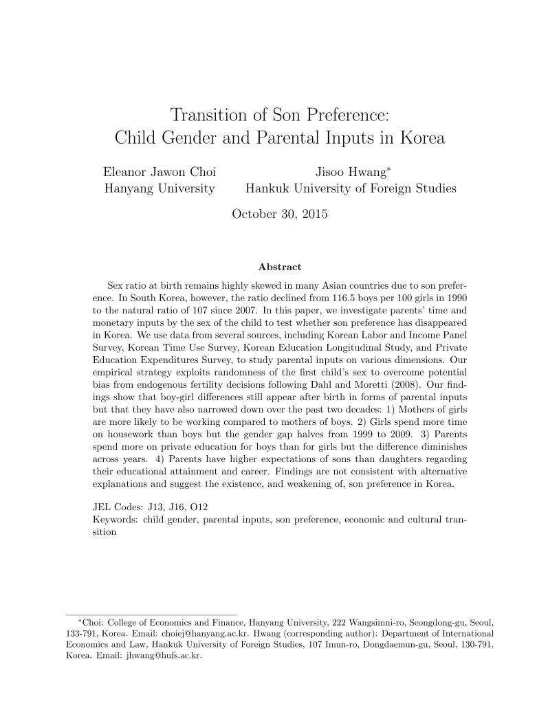
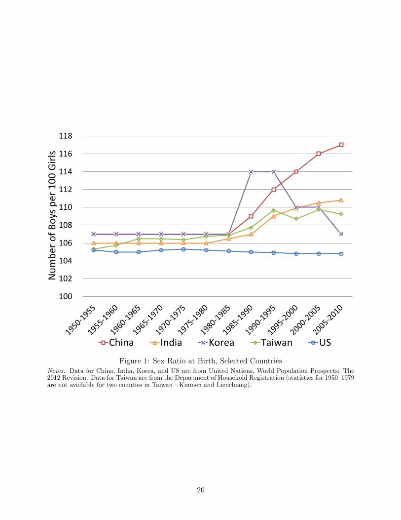
cieties. This is well represented by the grossly skewed sex ratio at birth: per 100 girls, 111
boys are born in China, 112 in India and Vietnam, and 113 in Hong Kong.1 Advanced
technologies that allow prenatal sex selection (e.g. ultra-sound) and the increasing desire for
smaller families have induced more parents to opt for their preferred—male—child.
*** Figure 1 here ***
However, South Korea (hereafter, Korea), which shares many of the traditional norms
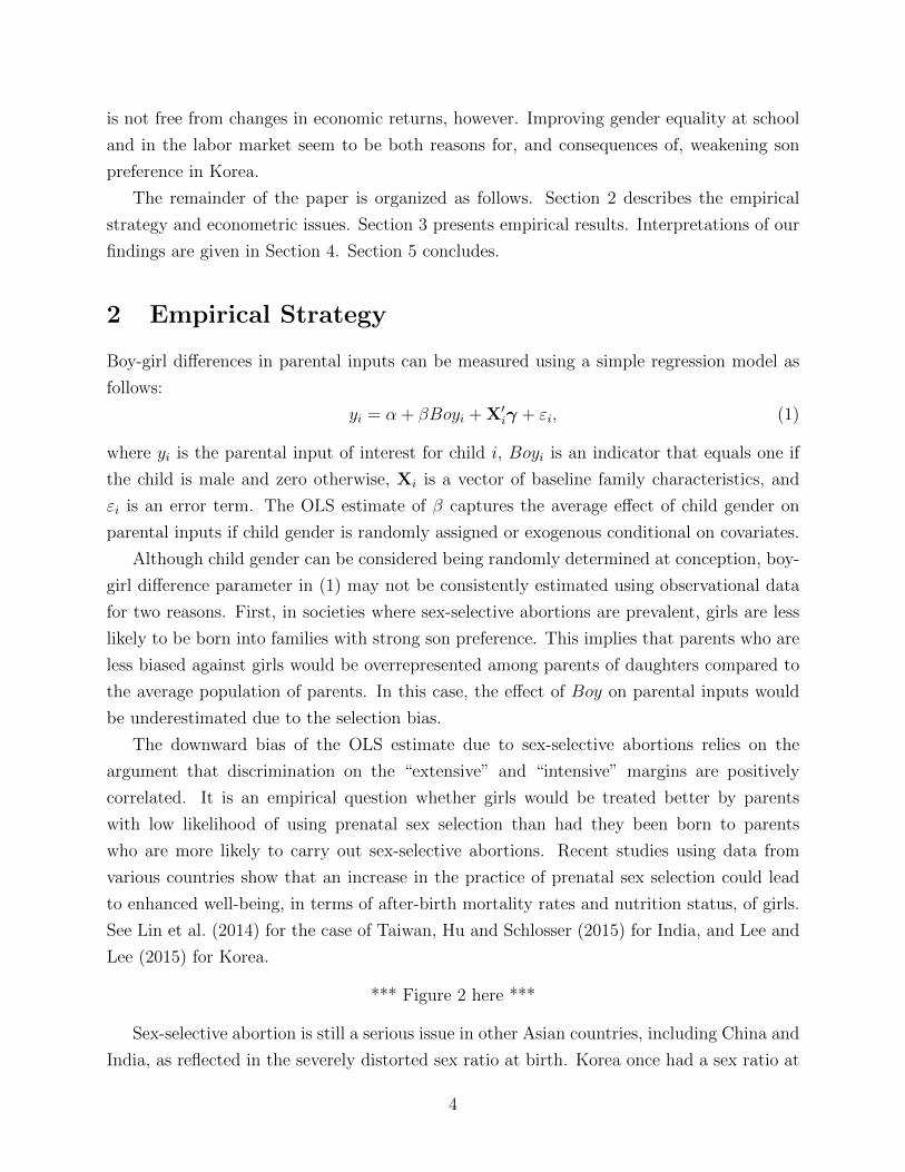
with nearby countries, seems to be heading towards gender neutrality. Sex ratio at birth
surpassed 116 in 1990, but has declined steadily until reaching 107 in 2007 and remaining
at natural levels since then (see Figure 1). Although there is still some bias among higher
order births, Korea is no longer a country with thousands of “missing women” (Sen, 1992;
Edlund and Lee, 2013).
Does the recovery of a natural sex ratio imply that son preference has disappeared in
Korea? This paper studies parent’s time and monetary inputs by child gender during the
period of decreasing sex ratio at birth. Although natural sex ratio at birth implies that
discrimination has diminished in the “extensive” margin of whether or not to have the child,
it may linger in the “intensive” margin after birth in the form of differential parental treat-
ment. Such parental behavior could result in non-trivial differences in child’s human capital
accumulation and career choices later on. Hence, we test whether there are boy-girl dif-
ferences in labor force participation of parents, child’s household work time, expenditures
on private out-of-school education, and parental expectations regarding their children’s aca-
demic achievement and occupational choices and further investigate whether some of these
measures changed during the past two decades.
Research on gender differences in parental investments has been conducted using data
from various countries. Previous studies look at the effect of child gender on fertility (Abre-
vaya, 2009; Almond et al., 2013; Edlund and Lee, 2013), marriage probability and stability
(Dahl and Moretti, 2008), parents’ labor supply (Lundberg and Rose, 2002; Choi et al.,
2008), health investments (Jayachandran and Kuziemko, 2011; Barcellos et al., 2014), and
educational inputs (Kang, 2011; Baker and Milligan, 2013). They find significant boy-girl
differences in both developing and developed countries, with the magnitude being larger in
developing countries.2
1Numbers are 2014 estimates available from the CIA World Factbook. For more details, see https://
www.cia.gov/library/publications/the-world-factbook/fields/2018.html (accessed May 29, 2015).2See Lundberg (2005) and Bharadwaj et al. (2015) for an overview of the literature on child gender and
family behavior.
1
Complementing existing literature, Korea is a particularly interesting case to study for the
following reasons. First, Korea is the only Asian country escaping the imbalanced sex ratio
at birth.3 The transitional experience could bridge the gap between studies on developing
and developed countries and have important implications for other Asian countries where son
preference remains strong to this day. Second, like the U.S., Korea’s college entrance rate is
now higher among women than men.4 However, Korea lags behind other developed countries
in female labor force participation and women’s relative wage (to men’s).5 Investigating
how much parents invest in their sons versus daughters, and hence understanding what
parents expect from their children may help answer some of the seemingly incongruent gap
in women’s educational attainment and their labor market outcomes.
To study parental time and monetary investments on various dimensions, we use data
from several sources, including Korean Labor and Income Panel Survey (KLIPS), Korean
Time Use Survey (KTUS), Korean Education Longitudinal Study (KELS), and Private Ed-
ucation Expenditures Survey (PEES).
Our empirical strategy exploits randomness of the first child’s sex to overcome potential
bias from endogenous fertility decisions, following Dahl and Moretti (2008). Throughout the
sample period of the past two decades, sex ratio at birth for first-born children shows no
evidence of sex-selective abortions. Also, our data shows no differences in various observable
characteristics between parents whose first child is male versus female. Even in the absence
of sex-selective abortion, however, child gender in higher order births may be correlated
with parents’ preference on child gender if there are parents employing son-biased fertility
stopping rules. Because girls in higher parity births are less likely to be born into families
biased against girls, boy-girl difference estimates from analyses including children of all birth
orders would possibly be biased downwards.
3In Taiwan and Hong Kong, sex ratio at birth had been increasing until very recently and suddenlydropped to around 107 during the past couple years. It is yet too early to determine whether sex imbalancehas improved in these countries, though. In Hong Kong, for example, the estimated sex ratio at birth for2014 is 113 – back to a highly distorted number. Korea is unique in terms that the ratio of males to femalesat birth has been declining for over two decades after soaring in the 1980s and reaching a peak in 1990. Theunique experience of Korea is also pointed out by The Economist in http://www.economist.com/node/
15606229 (accessed May 29, 2015). Consequently, in 2008, the Korean Constitutional Court overturned thelongstanding ban against the disclosure of a fetus’ gender. Sex ratio at birth has been remaining around thenatural ratio of 106 without the ban for the past several years and reached 105.3 in 2013.
4Girls’ college entrance rate surpassed boys’ in 2009 in Korea at 82.4 percent versus 81.6 percent (Statis-tical Yearbook of Education).
5According to OECD Employment Outlook 2013, employment to population ratio among women aged15–64 in Korea ranks 25th out of 34 OECD countries (at 53.5 percent), and the gender earnings gap remainsthe largest (at 37 percent).
2
Findings from KLIPS and KTUS provide evidence of important differences in time
allocations—both parent’s and child’s—by child gender. Mothers of girls are more likely
to be working compared to mothers of boys. We observe that the difference is not due to
characteristics before first childbirth but arises thereafter, as mothers are more likely to re-
turn to work when their first-born child is female. As for the time use of children, we find that
girls on average spend twice as much time as boys (of the same age) in housework activities
such as meal preparation and cleaning the house. The gender gap in housework time and
participation rate halves from 1999 to 2009, however, from 1 hour per week to half-an-hour
and from 18 percentage points to 9, respectively. Even at young ages, stereotypical gender
roles arise in the household, but decreasingly so in recent years.
The effects of offspring gender on parents’ monetary inputs and expectations are studied
using PEES and KELS. We focus on expenditures on children’s private out-of-school edu-
cation as they consist a major component of childrearing expenses in Korea.6 Parents are 3
percentage points more likely to make expenditures and spend 23 dollars more per month on
private out-of-school education in core academic subjects for their first-born boys than for
first-born girls at middle school age.7 Higher expenditures on boys seems to reflect higher
expectations regarding their academic achievement and career choices. Further analysis on
monthly private education spending in a broader range of academic subjects for children at
all grade levels indicates that the boy-girl difference has narrowed down from 10 dollars per
month in 2007 to 1 dollar in 2012.
How can we interpret these findings? We explore three potential explanations for gender
differential childcare: cost of raising girls are higher than boys, parents engage in compen-
satory behavior, or parents have son preference. The first hypothesis predicts that parents
with first-born girls would less likely have additional children than those with first-born
boys. This is rejected by the son-biased stopping rule. The compensatory behavior hy-
pothesis predicts that parents would spend more time and money on the child with greater
needs—on average, male. Additional analyses using educational data, however, suggest the
opposite: private education spending is positively correlated with child’s previous academic
performance.
Son preference is the most consistent explanation of all the results in this paper: parents
invest more in boys than girls because they gain higher utility from them. Such gender bias
6Authors’ calculation using PEES shows that about 79 percent of K-12 students received some kind ofprivate out-of-school education, such as private tutoring, group tutoring, cram schools, or online courses,in 2007–2012. A major differences in educational investment arises from expenditures from private out-of-school education because the vast majority of primary schools are public and the majority of public andprivate secondary schools are quite homogeneous in terms of curriculum and tuition rates.
7Core academic subjects include Korean, Math, and English.
3
is not free from changes in economic returns, however. Improving gender equality at school
and in the labor market seem to be both reasons for, and consequences of, weakening son
preference in Korea.
The remainder of the paper is organized as follows. Section 2 describes the empirical
strategy and econometric issues. Section 3 presents empirical results. Interpretations of our
findings are given in Section 4. Section 5 concludes.
2 Empirical Strategy
Boy-girl differences in parental inputs can be measured using a simple regression model as
follows:
yi = α + βBoyi + X′iγ + εi, (1)
where yi is the parental input of interest for child i, Boyi is an indicator that equals one if
the child is male and zero otherwise, Xi is a vector of baseline family characteristics, and
εi is an error term. The OLS estimate of β captures the average effect of child gender on
parental inputs if child gender is randomly assigned or exogenous conditional on covariates.
Although child gender can be considered being randomly determined at conception, boy-
girl difference parameter in (1) may not be consistently estimated using observational data
for two reasons. First, in societies where sex-selective abortions are prevalent, girls are less
likely to be born into families with strong son preference. This implies that parents who are
less biased against girls would be overrepresented among parents of daughters compared to
the average population of parents. In this case, the effect of Boy on parental inputs would
be underestimated due to the selection bias.
The downward bias of the OLS estimate due to sex-selective abortions relies on the
argument that discrimination on the “extensive” and “intensive” margins are positively
correlated. It is an empirical question whether girls would be treated better by parents
with low likelihood of using prenatal sex selection than had they been born to parents
who are more likely to carry out sex-selective abortions. Recent studies using data from
various countries show that an increase in the practice of prenatal sex selection could lead
to enhanced well-being, in terms of after-birth mortality rates and nutrition status, of girls.
See Lin et al. (2014) for the case of Taiwan, Hu and Schlosser (2015) for India, and Lee and
Lee (2015) for Korea.
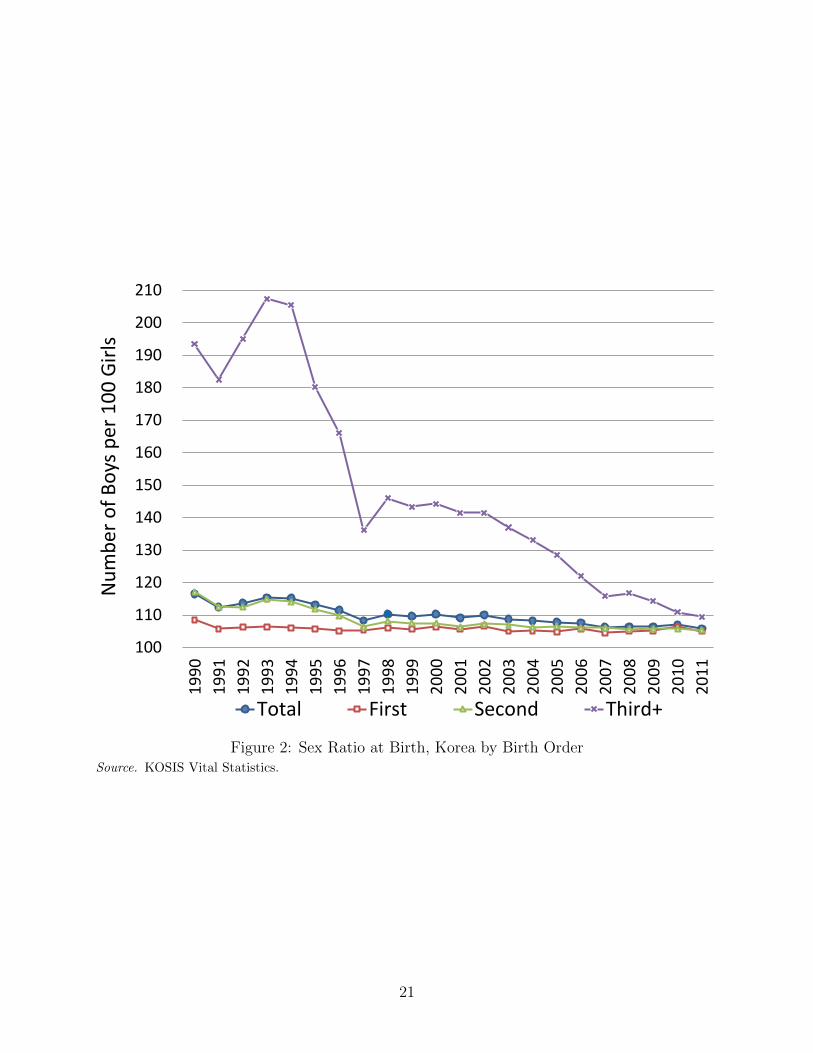
*** Figure 2 here ***
Sex-selective abortion is still a serious issue in other Asian countries, including China and
India, as reflected in the severely distorted sex ratio at birth. Korea once had a sex ratio at
4
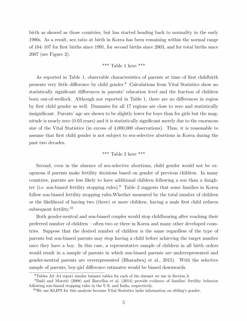
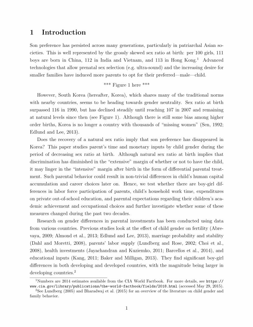
birth as skewed as those countries, but has started heading back to normality in the early
1990s. As a result, sex ratio at birth in Korea has been remaining within the normal range
of 104–107 for first births since 1991, for second births since 2003, and for total births since
2007 (see Figure 2).
*** Table 1 here ***
As reported in Table 1, observable characteristics of parents at time of first childbirth
presents very little difference by child gender.8 Calculations from Vital Statistics show no
statistically significant differences in parents’ education level and the fraction of children
born out-of-wedlock. Although not reported in Table 1, there are no differences in region
by first child gender as well. Dummies for all 17 regions are close to zero and statistically
insignificant. Parents’ age are shown to be slightly lower for boys than for girls but the mag-
nitude is nearly zero (0.03 years) and it is statistically significant merely due to the enormous
size of the Vital Statistics (in excess of 4,000,000 observations). Thus, it is reasonable to
assume that first child gender is not subject to sex-selective abortions in Korea during the
past two decades.
*** Table 2 here ***
Second, even in the absence of sex-selective abortions, child gender would not be ex-
ogenous if parents make fertility decisions based on gender of previous children. In many
countries, parents are less likely to have additional children following a son than a daugh-
ter (i.e. son-biased fertility stopping rules).9 Table 2 suggests that some families in Korea
follow son-biased fertility stopping rules.Whether measured by the total number of children
or the likelihood of having two (three) or more children, having a male first child reduces
subsequent fertility.10
Both gender-neutral and son-biased couples would stop childbearing after reaching their
preferred number of children – often two or three in Korea and many other developed coun-
tries. Suppose that the desired number of children is the same regardless of the type of
parents but son-biased parents may stop having a child before achieving the target number
once they have a boy. In this case, a representative sample of children in all birth orders
would result in a sample of parents in which son-biased parents are underrepresented and
gender-neutral parents are overrepresented (Bharadwaj et al., 2015). With the selective
sample of parents, boy-girl difference estimates would be biased downwards.
8Tables A2–A4 report similar balance tables for each of the dataset we use in Section 3.9Dahl and Moretti (2008) and Barcellos et al. (2014) provide evidence of families’ fertility behavior
following son-biased stopping rules in the U.S. and India, respectively.10We use KLIPS for this analysis because Vital Statistics lacks information on sibling’s gender.
5
The downward selection bias arising from son-biased fertility stopping rules becomes
more pronounced if the regression model (1) controls for the number of children. This
is because couples who have a son and stop having children before reaching their preferred
number of children would be effectively left out from the estimation sample of parents sharing
the same target number of children. Consequently, son-biased parents would be further
underrepresented conditioning on the number of children.
To address the selection bias from son-biased fertility stopping rules, we exploit ran-
domness of the first child’s gender following Dahl and Moretti (2008). Then, Boyi in the
regression model (1) indicates whether the first child is male and the estimation sample
would only consist of first-borns. In Korea, although there are signs of son-biased stopping
rules for higher-order births, there has been no evidence of prenatal sex selection among
first-born children since 1991. Thus, it is reasonable to assume that first-child gender is
exogenous during our sample period. Note that girls would end up having more siblings
than boys under son-biased fertility stopping rules. Thus, the identification strategy relying
on the first child’s gender consistently estimates the total effect of child gender on parental
inputs including any indirect effects through subsequent fertility choices that may depend
on the gender of the first-born child.11
3 Estimation Results
3.1 Time Inputs
3.1.1 The Effect of Child Gender on Mother’s Labor Supply
Parental time continues to be one of the most important investments to children. Despite
market substitutes for housework and childcare that have increasingly become available in
developed countries, parents’ time nurturing, educating, and playing with their child are
shown to significantly affect the child’s health and development (see for example, Amato
and Rivera, 1999; Datcher-Loury, 1988; Price, 2012; Zick et al., 2001).
Thus labor supply responses are commonly observed with the beginning of parenthood as
the value of the couple’s home time rises after childbirth. Changes in labor market outcomes
following parenthood need not be symmetrical between the couple, however, and in most
cases they are not. Comparing the relative value of home time and market time, the value of
women’s time at home becomes greater than men’s after childbirth due to both economic (e.g.
gender wage gap) and physical (e.g. breastfeeding) reasons (Becker, 1991). Thus mothers
11The total effect can be interpreted as including both partial and general equilibrium effects.
6
reduce their labor supply whereas fathers may slightly increase or decrease theirs.12
In Korea, the gender difference in labor supply response to childbirth is particularly stark:
men’s response remains minimal whereas many women quit work. Two factors attribute to
this divergence. First, Korea has one of the longest working hours among OECD countries.13
Second, due to the tradition of Confucianism, women are considered to be mainly responsible
for household activities, including childcare.
In this context, we study whether the first child’s sex has any effect on mother’s labor
supply. We use data from the Korean Labor Income Panel Study (KLIPS), a longitudinal
study of a representative sample of Korean households and individuals living in urban areas
(comparable to the PSID of the US). We use the first thirteen waves of KLIPS spanning
1998–2010 and construct a sample of households with mother-children pairs. To minimize
the probability that some of the children might have left the household, we use information
on relation to household head to identify the birth order of each child. As in Table 1, Table
A2 confirms that observable characteristics of would-be parents do not differ by first child’s
gender.
Table 3 reports the effect of first child gender on mother’s employment for a sample of
women who were observed some time before as well as after first childbirth. The outcome
variable is a dummy equal to 1 if a woman ever worked after her first childbirth.14 The
independent variable of interest is a dummy equal to 1 if the first child is a boy. The
coefficient on Boyi indicates that the probability a woman works after first childbirth is 8
percentage points lower when the first-born is male than when it is female. We obtain nearly
identical results when we shorten the time span and redefine the variables to ever worked
five years pre- and post- first childbirth.
*** Table 3 here ***
As mentioned in the previous section, the estimate of Boy includes any indirect effects
that operates through subsequent fertility choices. The finding in Table 3 is thus more
surprising given that Korean families are less likely to have additional children following a
son.12Lundberg and Rose (2002) discuss how the effects of children on men’s labor market outcomes are
ambiguous. As in Becker’s work, specialization would predict that husbands focus more on the labor market.On the other hand, the value of both parents’ time as inputs to childcare increase after a child is born; thiseffect would predict an increase in husbands’ time at home.
13Korea’s working hours has been the highest among all OECD countries from 2000 to 2007, and has beenthe second highest since 2008. According to 2013 statistics, yearly average working hours in Korea is 2,163hours whereas the OECD average is 1,770 hours.
14KLIPS divides respondents into two groups—employed and not employed (including not in labor force).An individual is defined as employed if he/she worked at least 1 hour for pay during the survey week, workedat least 18 hours as unpaid family worker, or had a job from which he/she was temporarily absent (e.g.,because of illness or vacation).
7
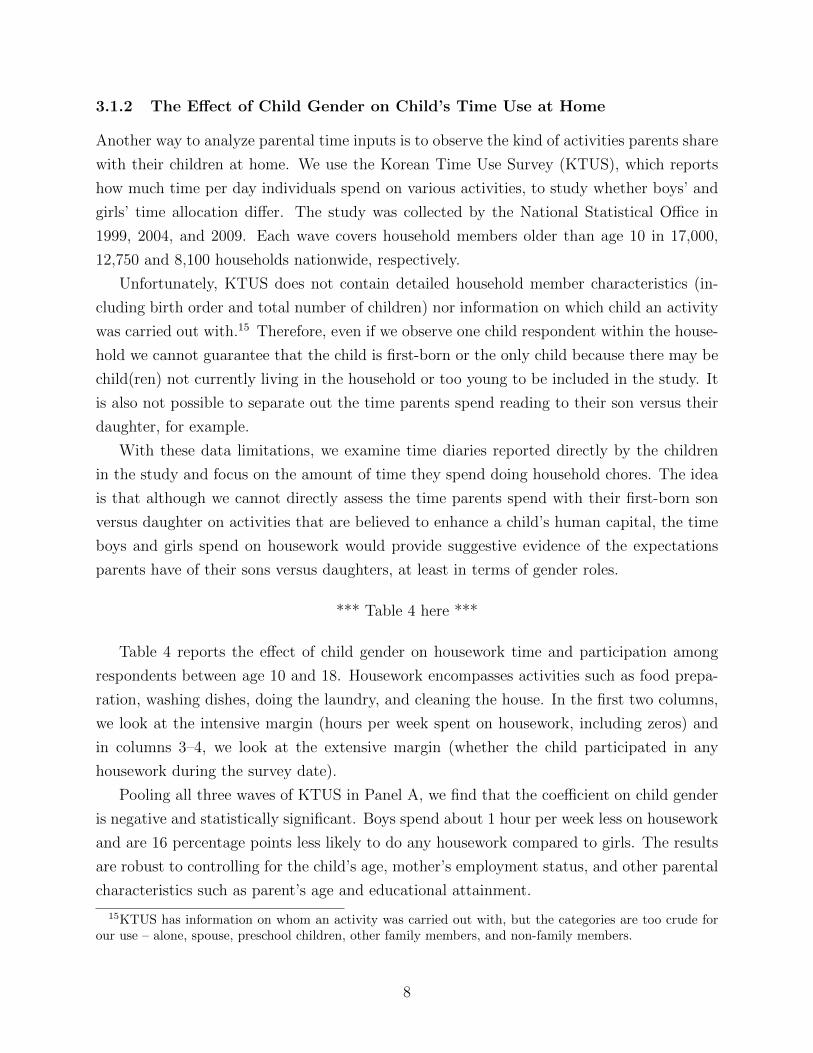
3.1.2 The Effect of Child Gender on Child’s Time Use at Home
Another way to analyze parental time inputs is to observe the kind of activities parents share
with their children at home. We use the Korean Time Use Survey (KTUS), which reports
how much time per day individuals spend on various activities, to study whether boys’ and
girls’ time allocation differ. The study was collected by the National Statistical Office in
1999, 2004, and 2009. Each wave covers household members older than age 10 in 17,000,
12,750 and 8,100 households nationwide, respectively.
Unfortunately, KTUS does not contain detailed household member characteristics (in-
cluding birth order and total number of children) nor information on which child an activity
was carried out with.15 Therefore, even if we observe one child respondent within the house-
hold we cannot guarantee that the child is first-born or the only child because there may be
child(ren) not currently living in the household or too young to be included in the study. It
is also not possible to separate out the time parents spend reading to their son versus their
daughter, for example.
With these data limitations, we examine time diaries reported directly by the children
in the study and focus on the amount of time they spend doing household chores. The idea
is that although we cannot directly assess the time parents spend with their first-born son
versus daughter on activities that are believed to enhance a child’s human capital, the time
boys and girls spend on housework would provide suggestive evidence of the expectations
parents have of their sons versus daughters, at least in terms of gender roles.
*** Table 4 here ***
Table 4 reports the effect of child gender on housework time and participation among
respondents between age 10 and 18. Housework encompasses activities such as food prepa-
ration, washing dishes, doing the laundry, and cleaning the house. In the first two columns,
we look at the intensive margin (hours per week spent on housework, including zeros) and
in columns 3–4, we look at the extensive margin (whether the child participated in any
housework during the survey date).
Pooling all three waves of KTUS in Panel A, we find that the coefficient on child gender
is negative and statistically significant. Boys spend about 1 hour per week less on housework
and are 16 percentage points less likely to do any housework compared to girls. The results
are robust to controlling for the child’s age, mother’s employment status, and other parental
characteristics such as parent’s age and educational attainment.
15KTUS has information on whom an activity was carried out with, but the categories are too crude forour use – alone, spouse, preschool children, other family members, and non-family members.
8

Panel B reveals another interesting pattern: gender difference in child’s housework time
and participation decreased in size across years. In 1999, boys spent about one hour less (per
week) on housework compared to girls whereas in 2004, the gap decreases to 0.7 hours and
in 2009, to 0.5 hours. Similar trend is observed in the extensive margin: the gender gap in
housework participation decreases from 18 percentage points in 1999 to 13 percentage points
in 2004 and to 9 percentage points in 2009. Although the size of the coefficients in 2009 are
still non-trivial given that the mean housework time and participation rate is only about 1
hour per week and 28 percent, respectively, a child’s gender role at home has become slightly
more equal during the ten-year period.
One note of caution is that the coefficient on child gender cannot be interpreted causally
because the KTUS sample is not restricted to first-born respondents. As discussed in Section
2, children from gender-biased parents would be underrepresented given that some Korean
families apply the son-biased fertility stopping rule. If we can assume that gender-biased
parents ask their daughters to help housework more than their sons (relative to gender-
neutral parents), the child gender effect may as well be larger than the estimates in Table
4.
3.2 Monetary Inputs and Expectations
Next, we investigate whether there are boy-girl differences in educational inputs in terms of
money and expectations. We focus on parents’ private education spending and expectations
on educational attainment and career choices. Here, private education indicates private
out-of-school education, such as private tutoring, cramming schools, and online courses, but
do not include private school fees. We use data from the Korean Education Longitudinal
Study (KELS) and the Private Education Expenditures Survey (PEES) to study educational
investments.
The KELS provides data on learning experiences and transitions to work of a nationally
representative sample of seventh-graders who were first surveyed in 2005. Similar to the
National Education Longitudinal Study of 1988 (NELS:1988) in the US, data are collected
from students, parents, teachers and school principals every year. We pool the first three
waves of the KELS and construct a sample of middle school students born in 1992 or 1993.16
The survey asks parents about monthly expenditures on private out-of-school education of
Korean, Math, and English, which are key subjects of the college entrance exam. The survey
also asks parents about the highest education level and occupational choices expected for
their child.
16We do not use later years of data because attrition rate becomes higher once sample members enter highschool in the fourth wave.
9
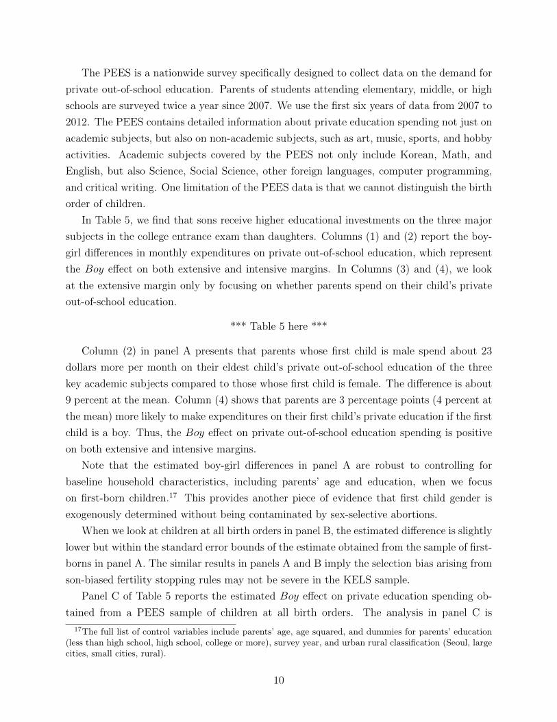
The PEES is a nationwide survey specifically designed to collect data on the demand for
private out-of-school education. Parents of students attending elementary, middle, or high
schools are surveyed twice a year since 2007. We use the first six years of data from 2007 to
2012. The PEES contains detailed information about private education spending not just on
academic subjects, but also on non-academic subjects, such as art, music, sports, and hobby
activities. Academic subjects covered by the PEES not only include Korean, Math, and
English, but also Science, Social Science, other foreign languages, computer programming,
and critical writing. One limitation of the PEES data is that we cannot distinguish the birth
order of children.
In Table 5, we find that sons receive higher educational investments on the three major
subjects in the college entrance exam than daughters. Columns (1) and (2) report the boy-
girl differences in monthly expenditures on private out-of-school education, which represent
the Boy effect on both extensive and intensive margins. In Columns (3) and (4), we look
at the extensive margin only by focusing on whether parents spend on their child’s private
out-of-school education.
*** Table 5 here ***
Column (2) in panel A presents that parents whose first child is male spend about 23
dollars more per month on their eldest child’s private out-of-school education of the three
key academic subjects compared to those whose first child is female. The difference is about
9 percent at the mean. Column (4) shows that parents are 3 percentage points (4 percent at
the mean) more likely to make expenditures on their first child’s private education if the first
child is a boy. Thus, the Boy effect on private out-of-school education spending is positive
on both extensive and intensive margins.
Note that the estimated boy-girl differences in panel A are robust to controlling for
baseline household characteristics, including parents’ age and education, when we focus
on first-born children.17 This provides another piece of evidence that first child gender is
exogenously determined without being contaminated by sex-selective abortions.
When we look at children at all birth orders in panel B, the estimated difference is slightly
lower but within the standard error bounds of the estimate obtained from the sample of first-
borns in panel A. The similar results in panels A and B imply the selection bias arising from
son-biased fertility stopping rules may not be severe in the KELS sample.
Panel C of Table 5 reports the estimated Boy effect on private education spending ob-
tained from a PEES sample of children at all birth orders. The analysis in panel C is
17The full list of control variables include parents’ age, age squared, and dummies for parents’ education(less than high school, high school, college or more), survey year, and urban rural classification (Seoul, largecities, small cities, rural).
10
restricted to middle school students from the PEES 2007 in order to make the estimation
sample comparable to the KELS sample in panel B. Also, private education spending is
restricted to the three subjects, Korean, Math, and English, to make the outcome variable
as consistent as possible with the one used in panel B. Compared to the estimates in panel
B, the effect on monthly expenditures is lower in terms of magnitude (18 dollars per month)
but similar in percentage terms (9 percent at the mean). On the extensive margin, similar
boy effect estimates are obtained.
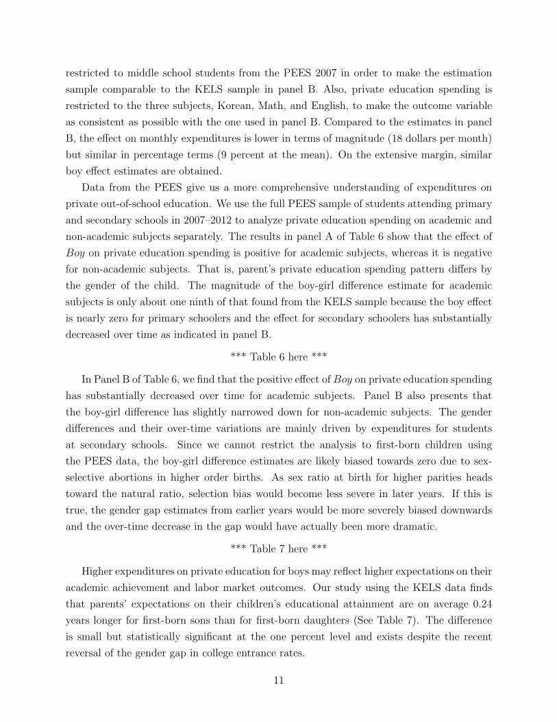
Data from the PEES give us a more comprehensive understanding of expenditures on
private out-of-school education. We use the full PEES sample of students attending primary
and secondary schools in 2007–2012 to analyze private education spending on academic and
non-academic subjects separately. The results in panel A of Table 6 show that the effect of
Boy on private education spending is positive for academic subjects, whereas it is negative
for non-academic subjects. That is, parent’s private education spending pattern differs by
the gender of the child. The magnitude of the boy-girl difference estimate for academic
subjects is only about one ninth of that found from the KELS sample because the boy effect
is nearly zero for primary schoolers and the effect for secondary schoolers has substantially
decreased over time as indicated in panel B.
*** Table 6 here ***
In Panel B of Table 6, we find that the positive effect of Boy on private education spending
has substantially decreased over time for academic subjects. Panel B also presents that
the boy-girl difference has slightly narrowed down for non-academic subjects. The gender
differences and their over-time variations are mainly driven by expenditures for students
at secondary schools. Since we cannot restrict the analysis to first-born children using
the PEES data, the boy-girl difference estimates are likely biased towards zero due to sex-
selective abortions in higher order births. As sex ratio at birth for higher parities heads
toward the natural ratio, selection bias would become less severe in later years. If this is
true, the gender gap estimates from earlier years would be more severely biased downwards
and the over-time decrease in the gap would have actually been more dramatic.
*** Table 7 here ***
Higher expenditures on private education for boys may reflect higher expectations on their
academic achievement and labor market outcomes. Our study using the KELS data finds
that parents’ expectations on their children’s educational attainment are on average 0.24
years longer for first-born sons than for first-born daughters (See Table 7). The difference
is small but statistically significant at the one percent level and exists despite the recent
reversal of the gender gap in college entrance rates.
11

*** Figure 3 here ***
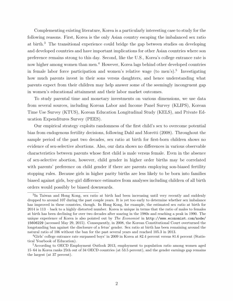
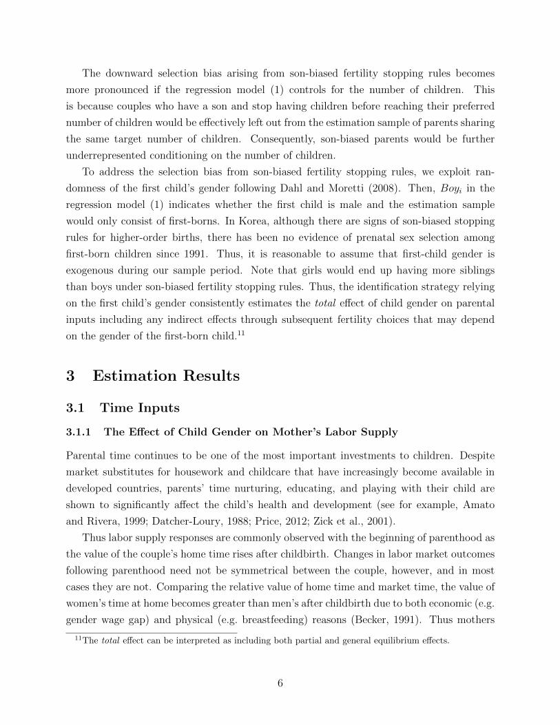
Figure 3 indicates that there is a substantial boy-girl difference in parents’ aspirations
for their children’s career choices. The KELS asks parents to select two occupations that
they would like their children to have in the future. We plot the fraction of parents who
select each occupation by first child’s gender. Parents of sons are more likely to select
high-wage professions or those that require advanced degrees, such as doctor, professor,
lawyer, and CEO, than parents of daughters. Parents of daughters tend to select female
dominated occupations, such as nurse and fashion stylist, or the ones with a high level of
job security, including teacher and pharmacist. Teacher is parents’ most preferred choice
for their daughter’s future occupation (selected by 54 percent). Although 20 percent of
parents state that they want their children to be scientists or engineers when their first
child is male, the number decreases to only three percent when their first child is female.
It seems that parents’ expectations on sons’ versus daughters’ career choices are generally
consistent with occupational gender stereotypes. The boy-girl difference in the fraction of
parents selecting each occupation is statistically significant at the one percent level for all
the listed occupations. Also, the estimated differences are robust to adding control variables
on baseline household characteristics.
4 Interpretations
The evidence in Section 3 reveals that whether we look at parental time inputs, monetary
inputs, or expectations regarding child’s education and occupation, boys and girls in Korea
are not treated equally at home. Although the gender gap has been narrowing over time, boys
are more likely to live with full-time housewife mothers (rather than working mothers), spend
much less time on household chores, receive more financial support for private education on
academic subjects, and are expected to obtain higher education and have higher-profile
careers.
Several interpretations are possible for why these differences arise. First, the cost of
raising boys and girls may differ. That is, child gender could directly affect the household
budget constraint. If marital costs are much higher for daughters than sons, for example,
parents would have to save more for the former. Even if parents do not have gender bias
and the “total” amount of parental input is the same for boys and girls, the “net” resources
available during childhood could differ by child gender in this case.
Second, boys may have greater needs than girls. Infant mortality is higher among boys
than girls in most countries including Korea.18 Boys are also known to have more attention
18According to KOSIS, infant mortality rate in 2014 is 3.2 for male and 2.8 for female infants. Extensive
12

difficulties and lower noncognitive skills compared to girls (see, for example, Bertrand and
Pan, 2013; Jacob, 2002; Ready et al., 2005). Depending on parent’s level of inequality
aversion, altruistic parents may engage in compensatory behavior by investing more in the
weaker—male—child (Behrman et al., 1982).
Lastly, parents may have son preference due to gender differences in economic returns,
psychic returns, or both. Despite the recent educational crossover and increases in female
labor force participation, Korea’s gender gap in wages remains one of the largest among
OECD countries at 37 percent.19 Parents would invest more in boys than girls if the former
is more likely to reap the benefits of these investments and is more reliable for old-age
support.
Gender differences in non-economic returns is also a possibility in a country like Korea,
where Confucianism dictates that only sons “carry on the family line.” For instance, the
eldest son is considered to be responsible for holding memorial services for the family’s
ancestors whereas married women are considered to belong to the husband’s household in
these ceremonies. These rituals have become less important nowadays, but they are still
carried out by most families and is often cited as a reason why married couples “need to
have a son.”
In discussing the son preference hypothesis, however, we do not attempt to separate out
these two types of returns. This is because it is very difficult, if not impossible, to isolate
“pure taste” from economic elements. Both parent’s preferences and child’s human capital
are endogenously formed and interact in reinforcing ways. If parents prefer boys to girls and
hence, invest more in them, boys will inevitably yield higher economic returns than girls in
the future, and would further justify parent’s bias for them. Whether (psychic) taste for sons
could have been formulated if not for the history of gender differences in economic returns
is highly questionable.20. Even Confucian traditions are closely related to the fact that only
men could provide for the family in the past.
Keeping this in mind, we now conduct additional exercises in an effort to distinguish
between the three channels—differential cost, compensatory behavior, and son preference.
If the first interpretation is true such that boys are less expensive to raise than girls, couples
whose first-born is male will be more likely to have another child compared to those whose
first-born is female due to an income effect (assuming that children are normal goods). This
research indicates that due to differences in genetic makeup, boys are biologically weaker and more susceptibleto diseases and premature death (see for example, Naeye et al., 1971; Waldron, 1983).
19Source: 2013 OECD Earnings Distribution Database.20Studies often use gender wage gaps or female labor force participation rates as proxies for a society’s
gender norms because they are highly correlated (see for example, Alesina and Giuliano, 2010; Fernandezand Fogli, 2009; Hwang, 2013). Within Korea as well, regions with lower sex ratio at birth have higherfemale wages (Lee, 2013)
13

is rejected in Korea, however, by the presence of son-biased stopping rules (Table 2). Also,
unlike countries like India where large dowries are common, the newlywed’s home (by far the
largest marriage expenditure) is usually supplied by the groom’s family in Korea whereas
other gifts are prepared by the bride’s. Although more gender-equal exchanges have been
increasing among recent marriages, differential cost is not in favor of boys in Korea.
As for compensatory behavior hypothesis, if this is true, we should observe parents spend-
ing more time and money on those children who are having difficulties. We should also find
that the effect of child’s deficit on parental input is stronger for boys than for girls given
that boys, on average, have more health and behavioral problems than girls.
In order to test whether parents engage in such behavior, we investigate how educa-
tional inputs differ by child’s academic performance from the previous year and whether the
difference depends on child’s gender using data from the KELS. The KELS data include
individual-level scores from a standardized test on Korean, Math, and English conducted
every year from 2005 to 2007. We construct a measure of child’s academic performance by
normalizing total scores on the three subjects to have zero mean and unit variance. We es-
timate a modified version of equation (1) by adding last year’s test score and its interaction
with child gender to the regression equation.
*** Table 8 here ***
Table 8 shows that educational inputs are positively correlated with child’s previous
academic performance. Conditioning on child gender, parents spend more on private out-
of-school education and expect a higher level of educational attainment when their children
perform better in school. Such pattern of parenting behavior would reinforce ability differ-
ences among children. The positive and statistically significant coefficient estimates on last
year’s test score (and its square) provides evidence of reinforcing, rather than compensat-
ing, behavior in parental investments. Although boys on average receive higher educational
investment compared to girls with the same level of academic achievement, we do not find
an additional boy effect on the reinforcing behavior.
We conduct a similar analysis using a self-reported measure of 6th-grade academic perfor-
mance available in the 2005 KELS data. Based on the self-reported measure, we classify 7th
graders into three groups – low, middle, and high achievers. Table A5 reports results from
regression analyses using these categorical variables of academic performance. Although es-
timates are not directly comparable, the results in Table A5 are qualitatively similar to those
in Table 8 above.
In addition, results from Table 6 and 7 also cast doubt on the claim that boys have
greater needs than girls. Parents expect longer educational years for their sons than their
14
daughters and focus on different subjects when spending on private education – academic
subjects for boys and arts for girls. If parents allocated monetary inputs unequally because
boys fared worse than girls in school (particularly in core subjects), it is difficult to explain
why parents then expect higher educational attainment for the former. There is no barrier
against women pursuing tertiary education in Korea; college entrance rates are higher for
girls than for boys since 2009. Thus parents’ expectations cannot be interpreted as reflecting
the status quo, either.
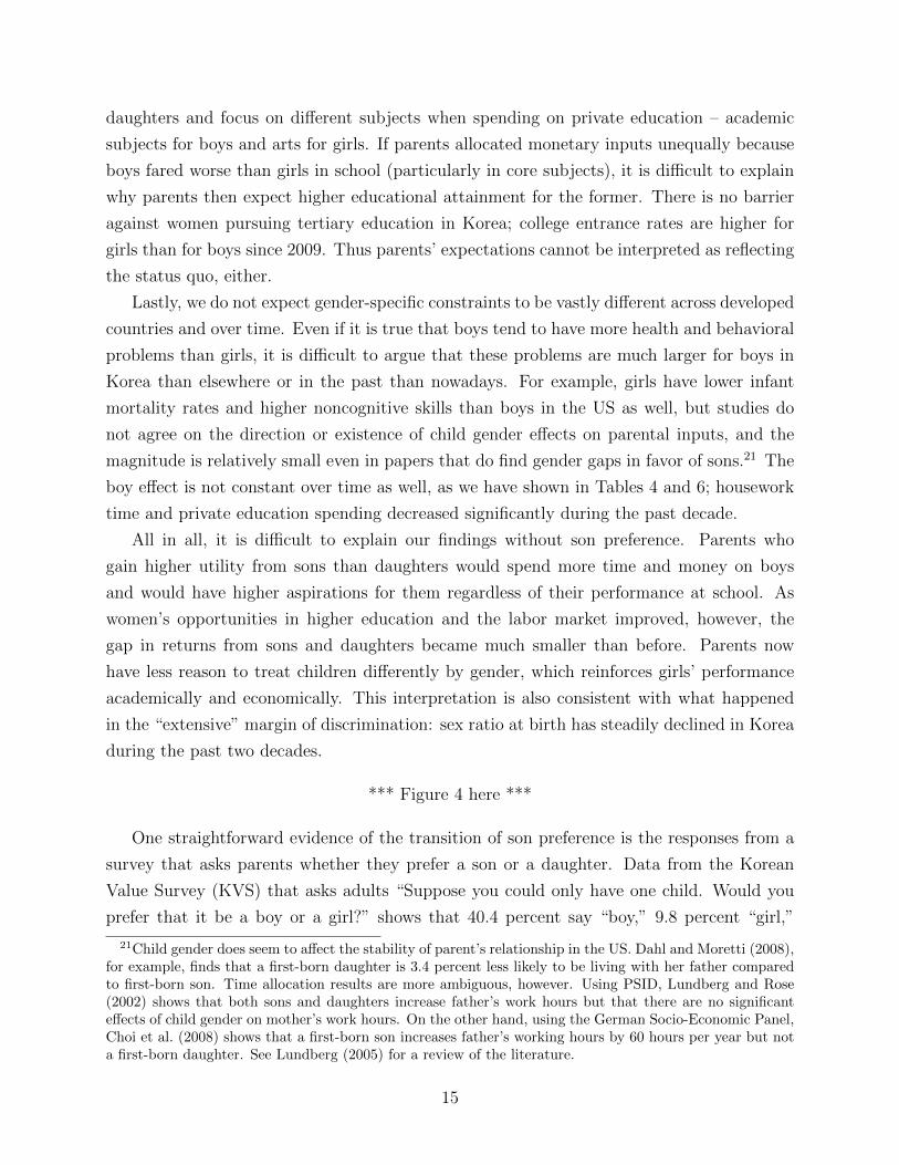
Lastly, we do not expect gender-specific constraints to be vastly different across developed
countries and over time. Even if it is true that boys tend to have more health and behavioral
problems than girls, it is difficult to argue that these problems are much larger for boys in
Korea than elsewhere or in the past than nowadays. For example, girls have lower infant
mortality rates and higher noncognitive skills than boys in the US as well, but studies do
not agree on the direction or existence of child gender effects on parental inputs, and the
magnitude is relatively small even in papers that do find gender gaps in favor of sons.21 The
boy effect is not constant over time as well, as we have shown in Tables 4 and 6; housework
time and private education spending decreased significantly during the past decade.
All in all, it is difficult to explain our findings without son preference. Parents who
gain higher utility from sons than daughters would spend more time and money on boys
and would have higher aspirations for them regardless of their performance at school. As
women’s opportunities in higher education and the labor market improved, however, the
gap in returns from sons and daughters became much smaller than before. Parents now
have less reason to treat children differently by gender, which reinforces girls’ performance
academically and economically. This interpretation is also consistent with what happened
in the “extensive” margin of discrimination: sex ratio at birth has steadily declined in Korea
during the past two decades.
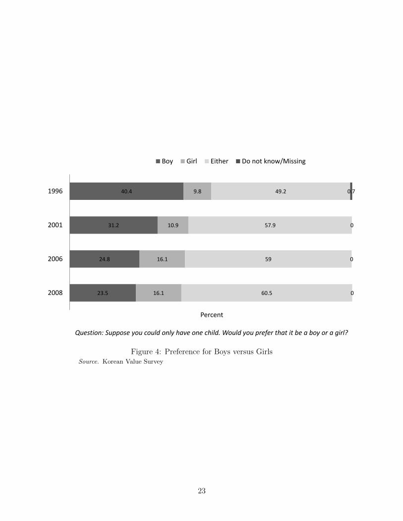
*** Figure 4 here ***
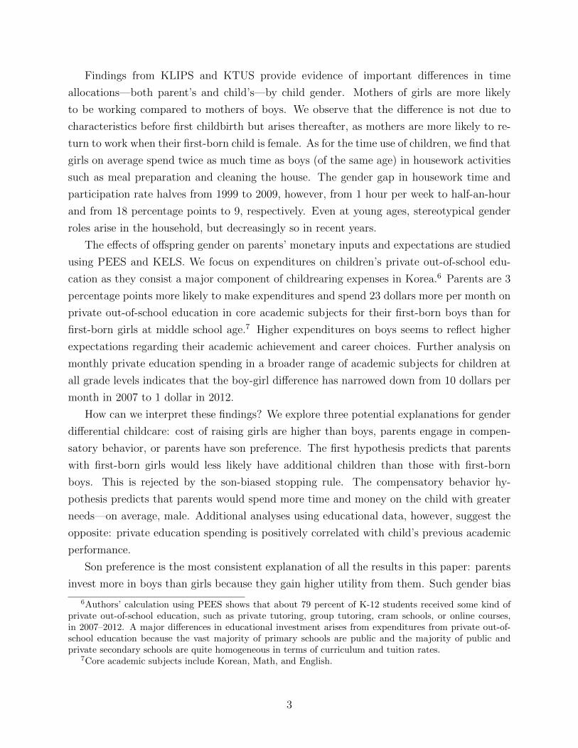
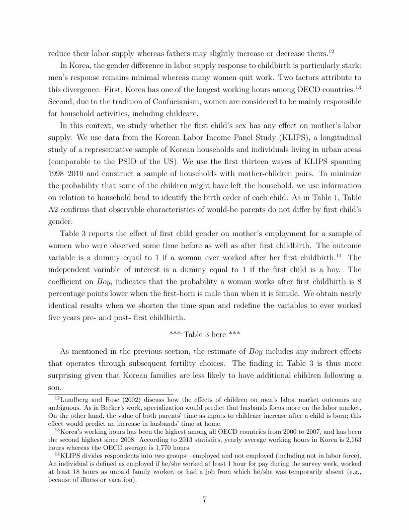
One straightforward evidence of the transition of son preference is the responses from a
survey that asks parents whether they prefer a son or a daughter. Data from the Korean
Value Survey (KVS) that asks adults “Suppose you could only have one child. Would you
prefer that it be a boy or a girl?” shows that 40.4 percent say “boy,” 9.8 percent “girl,”
21Child gender does seem to affect the stability of parent’s relationship in the US. Dahl and Moretti (2008),for example, finds that a first-born daughter is 3.4 percent less likely to be living with her father comparedto first-born son. Time allocation results are more ambiguous, however. Using PSID, Lundberg and Rose(2002) shows that both sons and daughters increase father’s work hours but that there are no significanteffects of child gender on mother’s work hours. On the other hand, using the German Socio-Economic Panel,Choi et al. (2008) shows that a first-born son increases father’s working hours by 60 hours per year but nota first-born daughter. See Lundberg (2005) for a review of the literature.
15
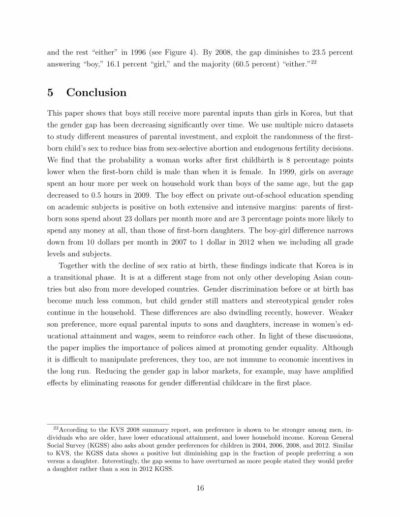
and the rest “either” in 1996 (see Figure 4). By 2008, the gap diminishes to 23.5 percent
answering “boy,” 16.1 percent “girl,” and the majority (60.5 percent) “either.”22
5 Conclusion
This paper shows that boys still receive more parental inputs than girls in Korea, but that
the gender gap has been decreasing significantly over time. We use multiple micro datasets
to study different measures of parental investment, and exploit the randomness of the first-
born child’s sex to reduce bias from sex-selective abortion and endogenous fertility decisions.
We find that the probability a woman works after first childbirth is 8 percentage points
lower when the first-born child is male than when it is female. In 1999, girls on average
spent an hour more per week on household work than boys of the same age, but the gap
decreased to 0.5 hours in 2009. The boy effect on private out-of-school education spending
on academic subjects is positive on both extensive and intensive margins: parents of first-
born sons spend about 23 dollars per month more and are 3 percentage points more likely to
spend any money at all, than those of first-born daughters. The boy-girl difference narrows
down from 10 dollars per month in 2007 to 1 dollar in 2012 when we including all grade
levels and subjects.
Together with the decline of sex ratio at birth, these findings indicate that Korea is in
a transitional phase. It is at a different stage from not only other developing Asian coun-
tries but also from more developed countries. Gender discrimination before or at birth has
become much less common, but child gender still matters and stereotypical gender roles
continue in the household. These differences are also dwindling recently, however. Weaker
son preference, more equal parental inputs to sons and daughters, increase in women’s ed-
ucational attainment and wages, seem to reinforce each other. In light of these discussions,
the paper implies the importance of polices aimed at promoting gender equality. Although
it is difficult to manipulate preferences, they too, are not immune to economic incentives in
the long run. Reducing the gender gap in labor markets, for example, may have amplified
effects by eliminating reasons for gender differential childcare in the first place.
22According to the KVS 2008 summary report, son preference is shown to be stronger among men, in-dividuals who are older, have lower educational attainment, and lower household income. Korean GeneralSocial Survey (KGSS) also asks about gender preferences for children in 2004, 2006, 2008, and 2012. Similarto KVS, the KGSS data shows a positive but diminishing gap in the fraction of people preferring a sonversus a daughter. Interestingly, the gap seems to have overturned as more people stated they would prefera daughter rather than a son in 2012 KGSS.
16
References
Abrevaya, Jason, “Are There Missing Girls in the United States? Evidence from BirthData,” American Economic Journal: Applied Economics, 2009, 1 (2), 1–34.
Alesina, Alberto and Paola Giuliano, “The Power of the Family,” Journal of EconomicGrowth, 2010, 15 (2), 93–125.
Almond, Douglas, Lena Edlund, and Kevin Milligan, “Son Preference and the Persis-tence of Culture: Evidence from South and East Asian Immigrants to Canada,” Populationand Development Review, 2013, 39 (1), 75–95.
Amato, Paul R and Fernando Rivera, “Paternal involvement and children’s behaviorproblems,” Journal of Marriage and the Family, 1999, pp. 375–384.
Baker, Michael and Kevin Milligan, “Boy-Girl Differences in Parental Time Invest-ments: Evidence from Three Countries,” Working Paper 18893, National Bureau of Eco-nomic Research March 2013.
Barcellos, Silvia Helena, Leandro S. Carvalho, and Adriana Lleras-Muney, “ChildGender and Parental Investments in India: Are Boys and Girls Treated Differently?,”American Economic Journal: Applied Economics, 2014, 6 (1), 157–189.
Becker, Gary S., A Treatise on the Family: Expanded Edition, Cambridge: Harvard Uni-versity Press, 1991.
Behrman, Jere R, Robert A Pollak, and Paul Taubman, “Parental preferences andprovision for progeny,” The Journal of Political Economy, 1982, pp. 52–73.
Bertrand, Marianne and Jessica Pan, “The Trouble with Boys: Social Influences and theGender Gap in Disruptive Behavior,” American Economic Journal: Applied Economics,2013, 5 (1), 32–64.
Bharadwaj, Prashant, Gordon B. Dahl, and Ketki Sheth, “Gender Discrimination inthe Family,” in Esther Redmount, ed., The Economics of the Family: How the HouseholdAffects Markets and Economic Growth, ABC-Clio, 2015, chapter 9, pp. 237–266.
Choi, Hyung-Jai, Jutta M. Joesch, and Shelly Lundberg, “Sons, daughters, wives,and the labour market outcomes of West German men,” Labour Economics, 2008, 15 (5),795 – 811.
Dahl, Gordon B. and Enrico Moretti, “The Demand for Sons,” The Review of EconomicStudies, 2008, 75, 1085–1120.
Datcher-Loury, Linda, “Effects of mother’s home time on children’s schooling,” The Re-view of Economics and Statistics, 1988, pp. 367–373.
Edlund, Lena and Chulhee Lee, “Son Preference, Sex Selection and Economic Develop-ment: The Case of South Korea,” Working Paper 18679, National Bureau of EconomicResearch January 2013.
17
Fernandez, Raquel and Alessandra Fogli, “Culture: An Empirical Investigation ofBeliefs, Work and Fertility,” American Economic Journal: Macroeconomics, 2009, 1 (1),146–177.
Hu, Luojia and Analıa Schlosser, “Prenatal Sex Selection and Girls’ Well-Being: Evi-dence from India,” The Economic Journal, 2015, 125 (587), 1227–1261.
Hwang, Jisoo, “The Second Shift: Assimilation in Housework Time Among Immigrants.”PhD dissertation, Harvard University 2013.
Jacob, Brian A, “Where the boys aren’t: Non-cognitive skills, returns to school and thegender gap in higher education,” Economics of Education Review, 2002, 21 (6), 589–598.
Jayachandran, Seema and Ilyana Kuziemko, “Why Do Mothers Breastfeed Girls Lessthan Boys? Evidence and Implications for Child Health in India,” The Quarterly Journalof Economics, 2011, 126 (3), 1485–1538.
Kang, Changhui, “Family Size and Educational Investments in Children: Evidence fromPrivate Tutoring Expenditures in South Korea,” Oxford Bulletin of Economics and Statis-tics, 2011, 73 (1), 59–78.
Lee, Chulhee, “Economic Change and Son Preference: Female Labor-Market Performancesand Sex Ratios at Birth in Korea,” Korea Review of Applied Economics, 2013, 15, 219–246.
and Esther Lee, “Son Preference, Sex-Selective Abortion, and Parental Investment inGirls in Korea: Evidence from the Year of the White Horse,” March 2015. Working Paper,Seoul National University.
Lin, Ming-Jen, Jin-Tan Liu, and Nancy Qian, “More Missing Women, Fewer DyingGirls: The Impact of Abortion on Sex Ratios at Birth and Excess Female Mortality inTaiwan,” Journal of the European Economic Association, August 2014, 12 (4), 899–926.
Lundberg, Shelly, “Sons, Daughters, and Parental Behaviour,” Oxford Review of Eco-nomic Policy, 2005, 21 (3), 340–356.
and Elaina Rose, “The Effects of Sons and Daughters on Men’s Labor Supply andWages,” Review of Economics and Statistics, 2002, 84 (2), 251–268.
Naeye, Richard L, Leslie S Burt, David L Wright, William A Blanc, and DorothyTatter, “Neonatal mortality, the male disadvantage,” Pediatrics, 1971, 48 (6), 902–906.
Price, Joseph, “The Effect of Parental Time Investments: Evidence from Natural Within-Family Variation,” Working Paper, National Bureau of Economic Research 2012.
Ready, Douglas D, Laura F LoGerfo, David T Burkam, and Valerie E Lee, “Ex-plaining Girls’ Advantage in Kindergarten Literacy Learning: Do Classroom BehaviorsMake a Difference?,” The Elementary School Journal, 2005, 106 (1), 21–38.
Sen, Amartya, “Missing women,” British Medical Journal, 1992, 304, 587–588.
18

Waldron, Ingrid, “Sex differences in human mortality: the role of genetic factors,” SocialScience & Medicine, 1983, 17 (6), 321–333.
Zick, Cathleen D, W Keith Bryant, and Eva Osterbacka, “Mothers’ employment,parental involvement, and the implications for intermediate child outcomes,” Social Sci-ence Research, 2001, 30 (1), 25–49.
19
100
102
104
106
108
110
112
114
116
118
Num
ber o
f Boy
s per
100
Girl
s
China India Korea Taiwan US
Figure 1: Sex Ratio at Birth, Selected CountriesNotes. Data for China, India, Korea, and US are from United Nations, World Population Prospects: The2012 Revision. Data for Taiwan are from the Department of Household Registration (statistics for 1950–1979are not available for two counties in Taiwan—Kinmen and Lienchiang).
20
100
110
120
130
140
150
160
170
180
190
200
210
1990
1991
1992
1993
1994
1995
1996
1997
1998
1999
2000
2001
2002
2003
2004
2005
2006
2007
2008
2009
2010
2011
Num
ber o
f Boy
s per
100
Girl
s
Total First Second Third+
Figure 2: Sex Ratio at Birth, Korea by Birth OrderSource. KOSIS Vital Statistics.
21

0 .2 .4 .6
Government employee
Teacher
Doctor
Professor/Researcher
Lawyer
Engineer
Scientist
Journalist/Broadcaster
CEO
Artist/Musician/Writer
Pharmacist
Nurse
Fashion stylist Boy Girl
Figure 3: Parents’ Expectations for Their Children’s Future Occupations, by First Child’sGenderNotes. Calculations using KELS 2005–2007. Each bar represents the fraction of parents who want theireldest children to have the given occupation. The Professor/Researcher category excludes scientists. Theboy-girl difference in the fraction of parents selecting each occupation is statistically significant at the 1%level for all the listed occupations. The estimated differences are robust to adding control variables listedunder Table 5.
22
23.5
24.8
31.2
40.4
16.1
16.1
10.9
9.8
60.5
59
57.9
49.2
0
0
0
0.7
2008
2006
2001
1996
Percent
Question: Suppose you could only have one child. Would you prefer that it be a boy or a girl?
Boy Girl Either Do not know/Missing
Figure 4: Preference for Boys versus GirlsSource. Korean Value Survey
23
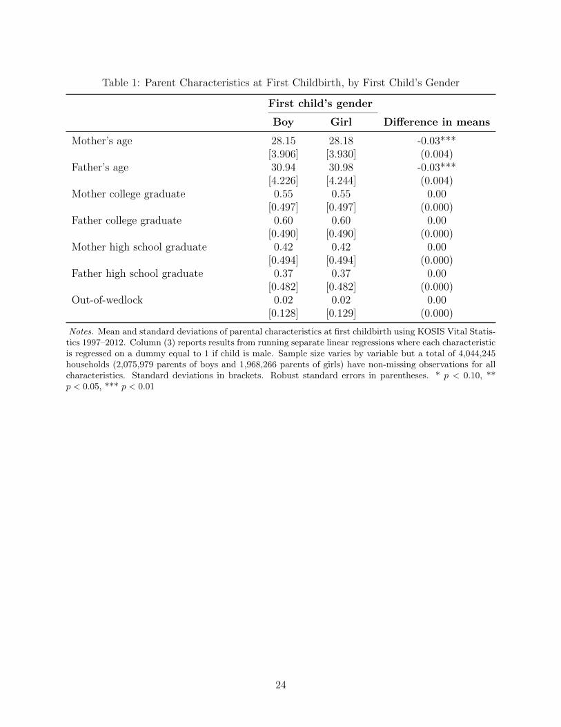
Table 1: Parent Characteristics at First Childbirth, by First Child’s Gender
First child’s gender
Boy Girl Difference in means
Mother’s age 28.15 28.18 -0.03***[3.906] [3.930] (0.004)
Father’s age 30.94 30.98 -0.03***[4.226] [4.244] (0.004)
Mother college graduate 0.55 0.55 0.00[0.497] [0.497] (0.000)
Father college graduate 0.60 0.60 0.00[0.490] [0.490] (0.000)
Mother high school graduate 0.42 0.42 0.00[0.494] [0.494] (0.000)
Father high school graduate 0.37 0.37 0.00[0.482] [0.482] (0.000)
Out-of-wedlock 0.02 0.02 0.00[0.128] [0.129] (0.000)
Notes. Mean and standard deviations of parental characteristics at first childbirth using KOSIS Vital Statis-tics 1997–2012. Column (3) reports results from running separate linear regressions where each characteristicis regressed on a dummy equal to 1 if child is male. Sample size varies by variable but a total of 4,044,245households (2,075,979 parents of boys and 1,968,266 parents of girls) have non-missing observations for allcharacteristics. Standard deviations in brackets. Robust standard errors in parentheses. * p < 0.10, **p < 0.05, *** p < 0.01
24
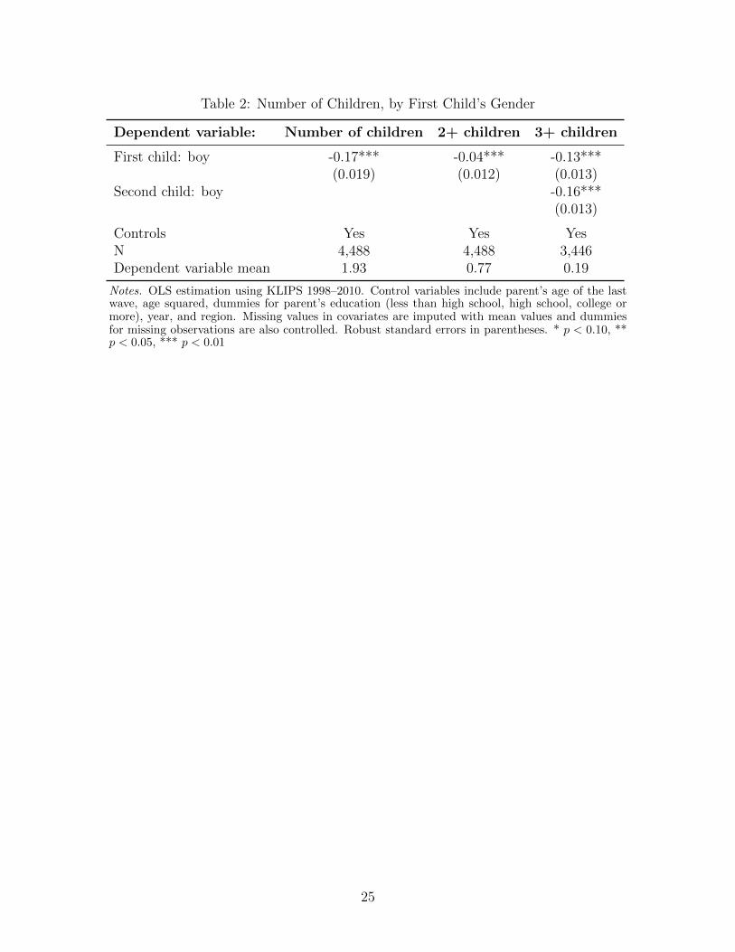
Table 2: Number of Children, by First Child’s Gender
Dependent variable: Number of children 2+ children 3+ children
First child: boy -0.17*** -0.04*** -0.13***(0.019) (0.012) (0.013)
Second child: boy -0.16***(0.013)
Controls Yes Yes YesN 4,488 4,488 3,446Dependent variable mean 1.93 0.77 0.19
Notes. OLS estimation using KLIPS 1998–2010. Control variables include parent’s age of the lastwave, age squared, dummies for parent’s education (less than high school, high school, college ormore), year, and region. Missing values in covariates are imputed with mean values and dummiesfor missing observations are also controlled. Robust standard errors in parentheses. * p < 0.10, **p < 0.05, *** p < 0.01
25
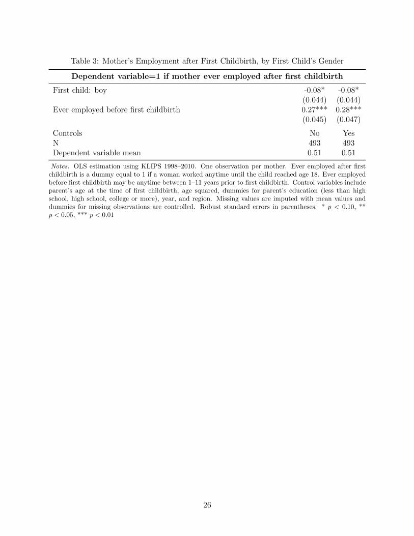
Table 3: Mother’s Employment after First Childbirth, by First Child’s Gender
Dependent variable=1 if mother ever employed after first childbirth
First child: boy -0.08* -0.08*(0.044) (0.044)
Ever employed before first childbirth 0.27*** 0.28***(0.045) (0.047)
Controls No YesN 493 493Dependent variable mean 0.51 0.51
Notes. OLS estimation using KLIPS 1998–2010. One observation per mother. Ever employed after firstchildbirth is a dummy equal to 1 if a woman worked anytime until the child reached age 18. Ever employedbefore first childbirth may be anytime between 1–11 years prior to first childbirth. Control variables includeparent’s age at the time of first childbirth, age squared, dummies for parent’s education (less than highschool, high school, college or more), year, and region. Missing values are imputed with mean values anddummies for missing observations are controlled. Robust standard errors in parentheses. * p < 0.10, **p < 0.05, *** p < 0.01
26
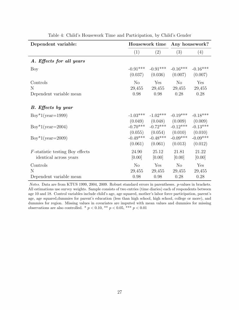
Table 4: Child’s Housework Time and Participation, by Child’s Gender
Dependent variable: Housework time Any housework?
(1) (2) (3) (4)
A. Effects for all years
Boy -0.91*** -0.91*** -0.16*** -0.16***(0.037) (0.036) (0.007) (0.007)
Controls No Yes No YesN 29,455 29,455 29,455 29,455Dependent variable mean 0.98 0.98 0.28 0.28
B. Effects by year
Boy*1(year=1999) -1.03*** -1.02*** -0.19*** -0.18***(0.049) (0.048) (0.009) (0.009)
Boy*1(year=2004) -0.70*** -0.72*** -0.12*** -0.13***(0.055) (0.054) (0.010) (0.010)
Boy*1(year=2009) -0.49*** -0.48*** -0.09*** -0.09***(0.061) (0.061) (0.013) (0.012)
F -statistic testing Boy effects 24.90 25.12 21.81 21.22identical across years [0.00] [0.00] [0.00] [0.00]
Controls No Yes No YesN 29,455 29,455 29,455 29,455Dependent variable mean 0.98 0.98 0.28 0.28
Notes. Data are from KTUS 1999, 2004, 2009. Robust standard errors in parentheses. p-values in brackets.All estimations use survey weights. Sample consists of two entries (time diaries) each of respondents betweenage 10 and 18. Control variables include child’s age, age squared, mother’s labor force participation, parent’sage, age squared,dummies for parent’s education (less than high school, high school, college or more), anddummies for region. Missing values in covariates are imputed with mean values and dummies for missingobservations are also controlled. * p < 0.10, ** p < 0.05, *** p < 0.01
27
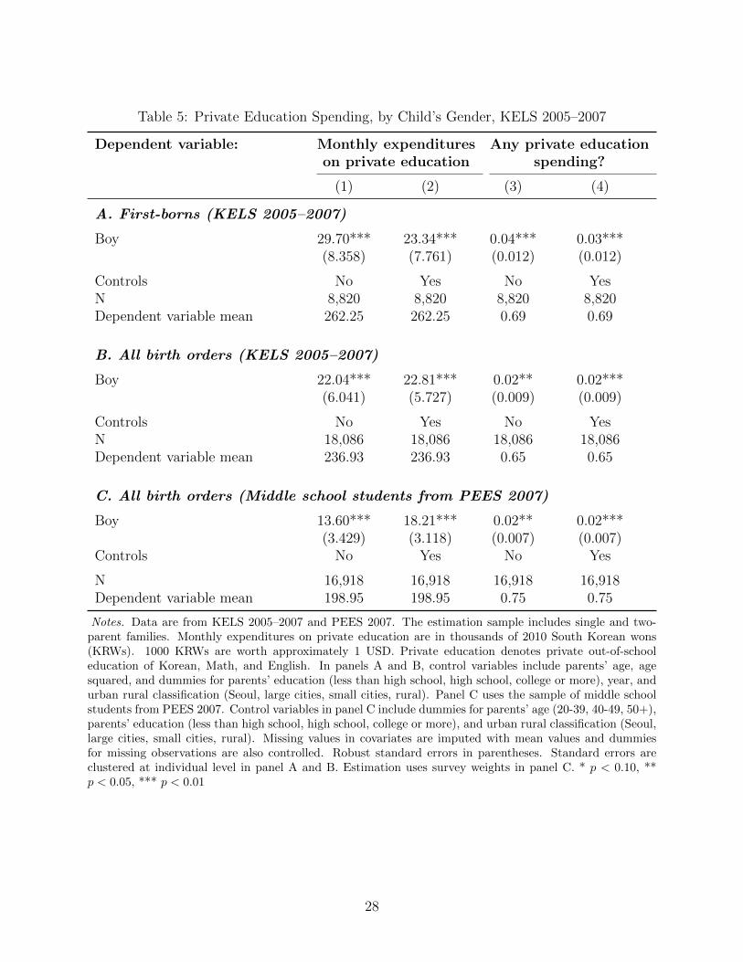
Table 5: Private Education Spending, by Child’s Gender, KELS 2005–2007
Dependent variable: Monthly expenditures Any private educationon private education spending?
(1) (2) (3) (4)
A. First-borns (KELS 2005–2007)
Boy 29.70*** 23.34*** 0.04*** 0.03***(8.358) (7.761) (0.012) (0.012)
Controls No Yes No YesN 8,820 8,820 8,820 8,820Dependent variable mean 262.25 262.25 0.69 0.69
B. All birth orders (KELS 2005–2007)
Boy 22.04*** 22.81*** 0.02** 0.02***(6.041) (5.727) (0.009) (0.009)
Controls No Yes No YesN 18,086 18,086 18,086 18,086Dependent variable mean 236.93 236.93 0.65 0.65
C. All birth orders (Middle school students from PEES 2007)
Boy 13.60*** 18.21*** 0.02** 0.02***(3.429) (3.118) (0.007) (0.007)
Controls No Yes No Yes
N 16,918 16,918 16,918 16,918Dependent variable mean 198.95 198.95 0.75 0.75
Notes. Data are from KELS 2005–2007 and PEES 2007. The estimation sample includes single and two-parent families. Monthly expenditures on private education are in thousands of 2010 South Korean wons(KRWs). 1000 KRWs are worth approximately 1 USD. Private education denotes private out-of-schooleducation of Korean, Math, and English. In panels A and B, control variables include parents’ age, agesquared, and dummies for parents’ education (less than high school, high school, college or more), year, andurban rural classification (Seoul, large cities, small cities, rural). Panel C uses the sample of middle schoolstudents from PEES 2007. Control variables in panel C include dummies for parents’ age (20-39, 40-49, 50+),parents’ education (less than high school, high school, college or more), and urban rural classification (Seoul,large cities, small cities, rural). Missing values in covariates are imputed with mean values and dummiesfor missing observations are also controlled. Robust standard errors in parentheses. Standard errors areclustered at individual level in panel A and B. Estimation uses survey weights in panel C. * p < 0.10, **p < 0.05, *** p < 0.01
28
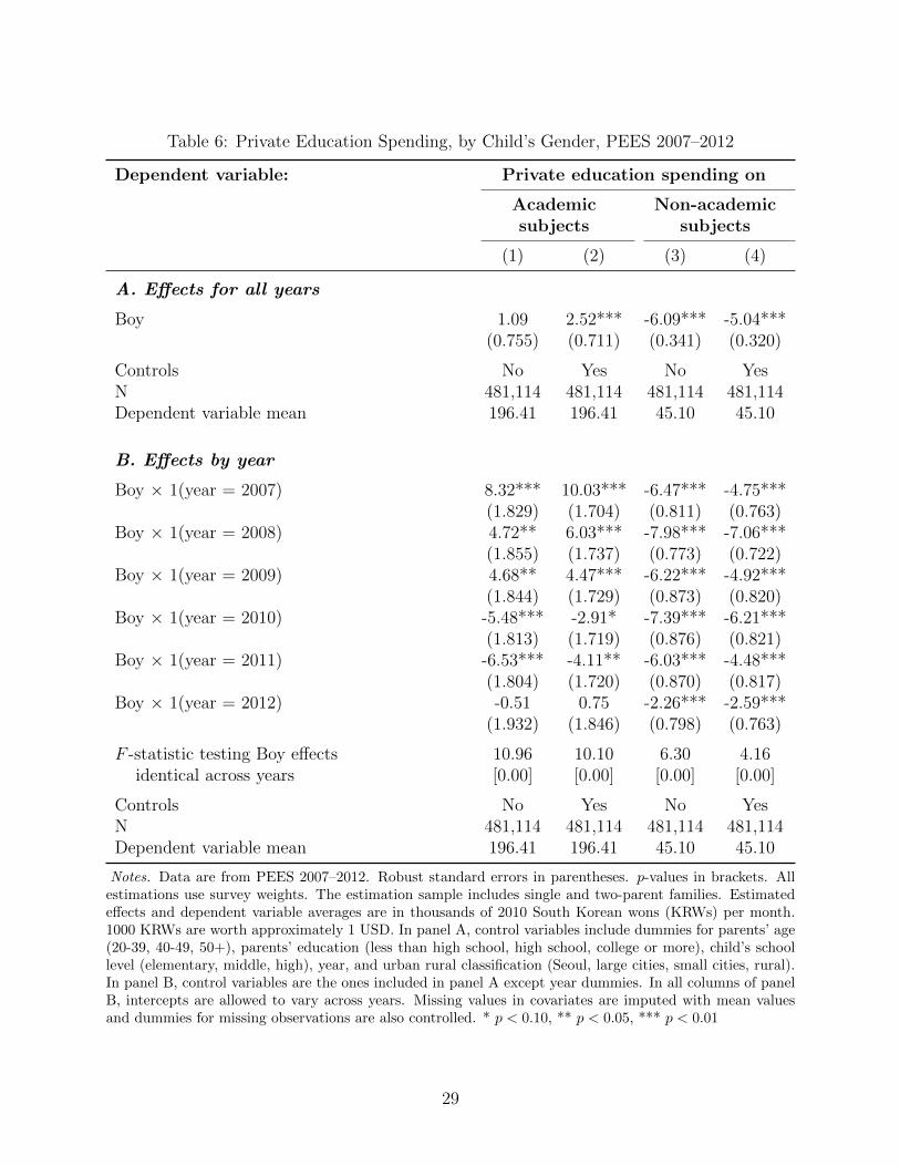
Table 6: Private Education Spending, by Child’s Gender, PEES 2007–2012
Dependent variable: Private education spending on
Academic Non-academicsubjects subjects
(1) (2) (3) (4)
A. Effects for all years
Boy 1.09 2.52*** -6.09*** -5.04***(0.755) (0.711) (0.341) (0.320)
Controls No Yes No YesN 481,114 481,114 481,114 481,114Dependent variable mean 196.41 196.41 45.10 45.10
B. Effects by year
Boy × 1(year = 2007) 8.32*** 10.03*** -6.47*** -4.75***(1.829) (1.704) (0.811) (0.763)
Boy × 1(year = 2008) 4.72** 6.03*** -7.98*** -7.06***(1.855) (1.737) (0.773) (0.722)
Boy × 1(year = 2009) 4.68** 4.47*** -6.22*** -4.92***(1.844) (1.729) (0.873) (0.820)
Boy × 1(year = 2010) -5.48*** -2.91* -7.39*** -6.21***(1.813) (1.719) (0.876) (0.821)
Boy × 1(year = 2011) -6.53*** -4.11** -6.03*** -4.48***(1.804) (1.720) (0.870) (0.817)
Boy × 1(year = 2012) -0.51 0.75 -2.26*** -2.59***(1.932) (1.846) (0.798) (0.763)
F -statistic testing Boy effects 10.96 10.10 6.30 4.16identical across years [0.00] [0.00] [0.00] [0.00]
Controls No Yes No YesN 481,114 481,114 481,114 481,114Dependent variable mean 196.41 196.41 45.10 45.10
Notes. Data are from PEES 2007–2012. Robust standard errors in parentheses. p-values in brackets. Allestimations use survey weights. The estimation sample includes single and two-parent families. Estimatedeffects and dependent variable averages are in thousands of 2010 South Korean wons (KRWs) per month.1000 KRWs are worth approximately 1 USD. In panel A, control variables include dummies for parents’ age(20-39, 40-49, 50+), parents’ education (less than high school, high school, college or more), child’s schoollevel (elementary, middle, high), year, and urban rural classification (Seoul, large cities, small cities, rural).In panel B, control variables are the ones included in panel A except year dummies. In all columns of panelB, intercepts are allowed to vary across years. Missing values in covariates are imputed with mean valuesand dummies for missing observations are also controlled. * p < 0.10, ** p < 0.05, *** p < 0.01
29
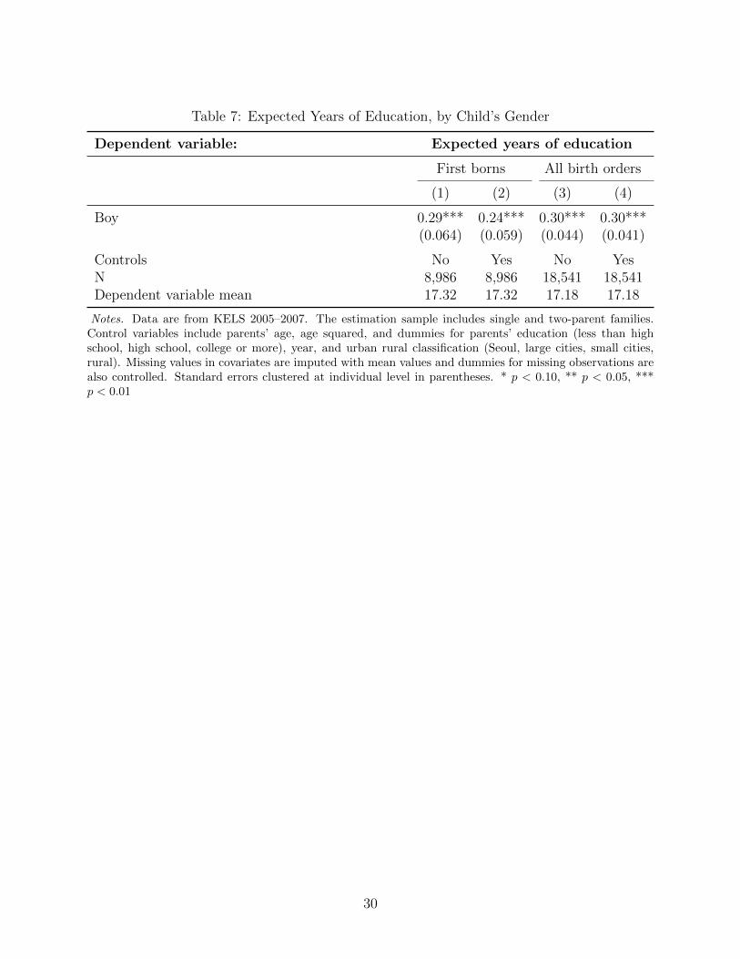
Table 7: Expected Years of Education, by Child’s Gender
Dependent variable: Expected years of education
First borns All birth orders
(1) (2) (3) (4)
Boy 0.29*** 0.24*** 0.30*** 0.30***(0.064) (0.059) (0.044) (0.041)
Controls No Yes No YesN 8,986 8,986 18,541 18,541Dependent variable mean 17.32 17.32 17.18 17.18
Notes. Data are from KELS 2005–2007. The estimation sample includes single and two-parent families.Control variables include parents’ age, age squared, and dummies for parents’ education (less than highschool, high school, college or more), year, and urban rural classification (Seoul, large cities, small cities,rural). Missing values in covariates are imputed with mean values and dummies for missing observations arealso controlled. Standard errors clustered at individual level in parentheses. * p < 0.10, ** p < 0.05, ***p < 0.01
30
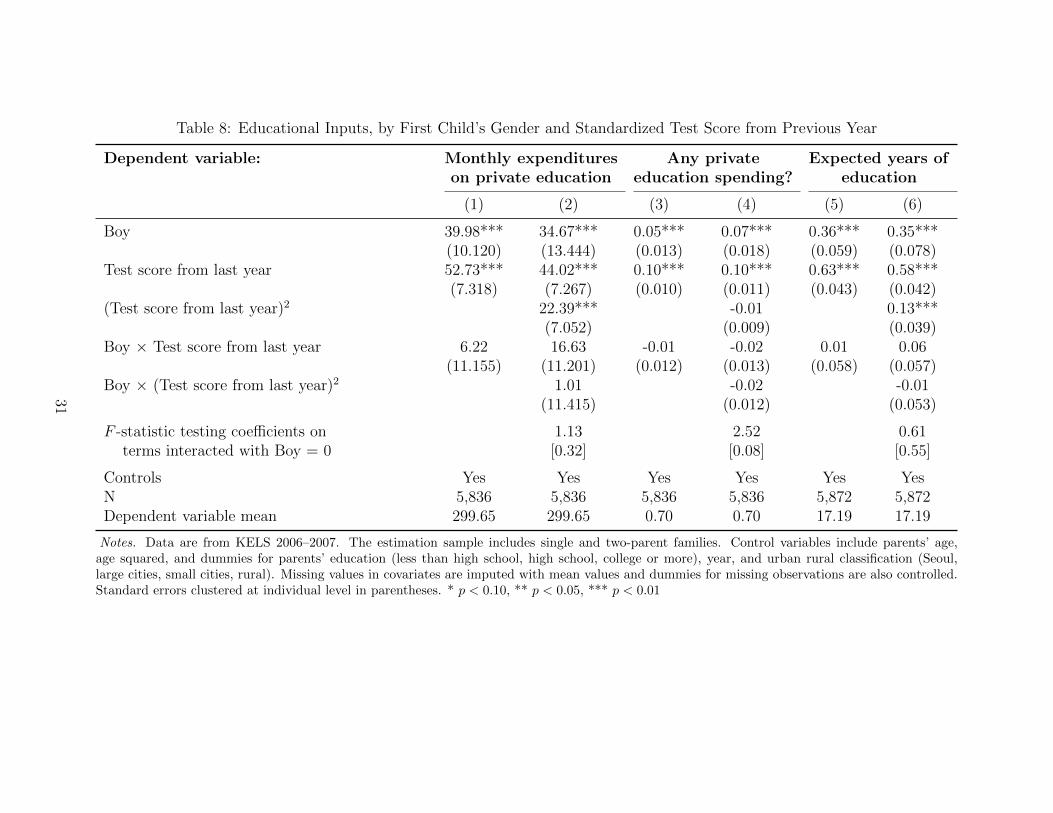
Table 8: Educational Inputs, by First Child’s Gender and Standardized Test Score from Previous Year
Dependent variable: Monthly expenditures Any private Expected years ofon private education education spending? education
(1) (2) (3) (4) (5) (6)
Boy 39.98*** 34.67*** 0.05*** 0.07*** 0.36*** 0.35***(10.120) (13.444) (0.013) (0.018) (0.059) (0.078)
Test score from last year 52.73*** 44.02*** 0.10*** 0.10*** 0.63*** 0.58***(7.318) (7.267) (0.010) (0.011) (0.043) (0.042)
(Test score from last year)2 22.39*** -0.01 0.13***(7.052) (0.009) (0.039)
Boy × Test score from last year 6.22 16.63 -0.01 -0.02 0.01 0.06(11.155) (11.201) (0.012) (0.013) (0.058) (0.057)
Boy × (Test score from last year)2 1.01 -0.02 -0.01(11.415) (0.012) (0.053)
F -statistic testing coefficients on 1.13 2.52 0.61terms interacted with Boy = 0 [0.32] [0.08] [0.55]
Controls Yes Yes Yes Yes Yes YesN 5,836 5,836 5,836 5,836 5,872 5,872Dependent variable mean 299.65 299.65 0.70 0.70 17.19 17.19
Notes. Data are from KELS 2006–2007. The estimation sample includes single and two-parent families. Control variables include parents’ age,age squared, and dummies for parents’ education (less than high school, high school, college or more), year, and urban rural classification (Seoul,large cities, small cities, rural). Missing values in covariates are imputed with mean values and dummies for missing observations are also controlled.Standard errors clustered at individual level in parentheses. * p < 0.10, ** p < 0.05, *** p < 0.01
31
Appendix
A Data Description
A.1 Vital Statistics
A.2 Korean Labor and Income Panel Survey (KLIPS)
KLIPS is a longitudinal study of a representative sample of Korean households and individ-uals living in urban areas. It was initiated by the Korea Labor Institute in 1998 and themost recent, 13th wave, was conducted in 2010. The 1st wave composed of 5,000 householdsand their members aged 15 or older.
Using household ID, person ID, and relation to household head, we identify the first-bornchild and the child’s mother. Father is defined based on spousal relationship with regardsto the mother. Households with only grown-ups (no child or youngest child older than 18),with adopted children, or with a change in mother’s ID anytime during the sample period(from divorce, remarriage, etc.) are excluded. Year relative to first childbirth is extrapolatedusing the first child’s age.
A.3 Korean Time Use Survey (KTUS)
Korea’s Time Use Survey is collected by the National Statistical Office every five yearsbeginning from 1999 and provides nationally representative data of how Koreans spend theirtime. Household members older than age 10 record the time they spend on various activities(both main and secondary) during two survey dates.
The dependent variable, housework time, is constructed from respondents’ time spent on“Household Activities” as the main activity. Household activities corresponds to the samecategory in the Bureau of Labor Statistics time use data and includes activities such ashousework, food and drink preparation and clean-up, interior maintenance, exterior main-tenance, vehicle maintenance, and household management. It does not include time spenton caring for children or other family members. Time diaries are reported in minutes. Forconvenience, we convert measures to weekly hours by multiplying by 7 (days) and dividingby 60 (minutes).
The data does not provide information on child’s birth order, total number of childrenin the household, or which child a parent carried out an activity with. Thus we study childrespondents’ (ages 10–18) time diaries directly. Household characteristics, including parent’sdemographics, are matched to child entries using household ID, person ID, and relation tohousehold head variables. Child respondents who could not be matched with parent IDwere excluded from the sample. Estimation uses survey weights, which takes into accountrespondent’s sex, age, and week(end) day of survey.
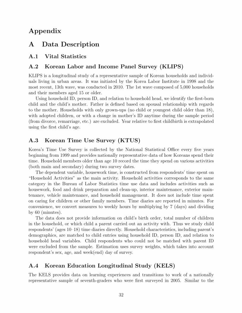
A.4 Korean Education Longitudinal Study (KELS)
The KELS provides data on learning experiences and transitions to work of a nationallyrepresentative sample of seventh-graders who were first surveyed in 2005. Similar to the
32

National Education Longitudinal Study of 1988 (NELS:1988) in the US, data are collectedfrom students, parents, teachers and school principals every year. We pool the first threewaves of the KELS and construct a sample of middle school students born in 1992 or 1993.We do not use later years of data because attrition rate becomes higher once sample membersenter high school in the fourth wave. The sample members are supposed to be followed upevery year until they become thirty years old.
A.5 Private Education Expenditures Survey (PEES)
The PEES is a nationwide survey specifically designed to collect data on the demand forprivate out-of-school education. Parents of students attending elementary, middle, or highschools are surveyed twice a year since 2007. We use the first six years of data from 2007 to2012. The PEES contains detailed information about private education spending not just onacademic subjects, but also on non-academic subjects, such as art, music, sports, and hobbyactivities. Academic subjects covered by the PEES not only include Korean, Math, andEnglish, but also Science, Social Science, other foreign languages, computer programming,and critical writing. One limitation of the PEES data is that we cannot distinguish the birthorder of children.
A.6 Korean Value Survey (KVS)
33
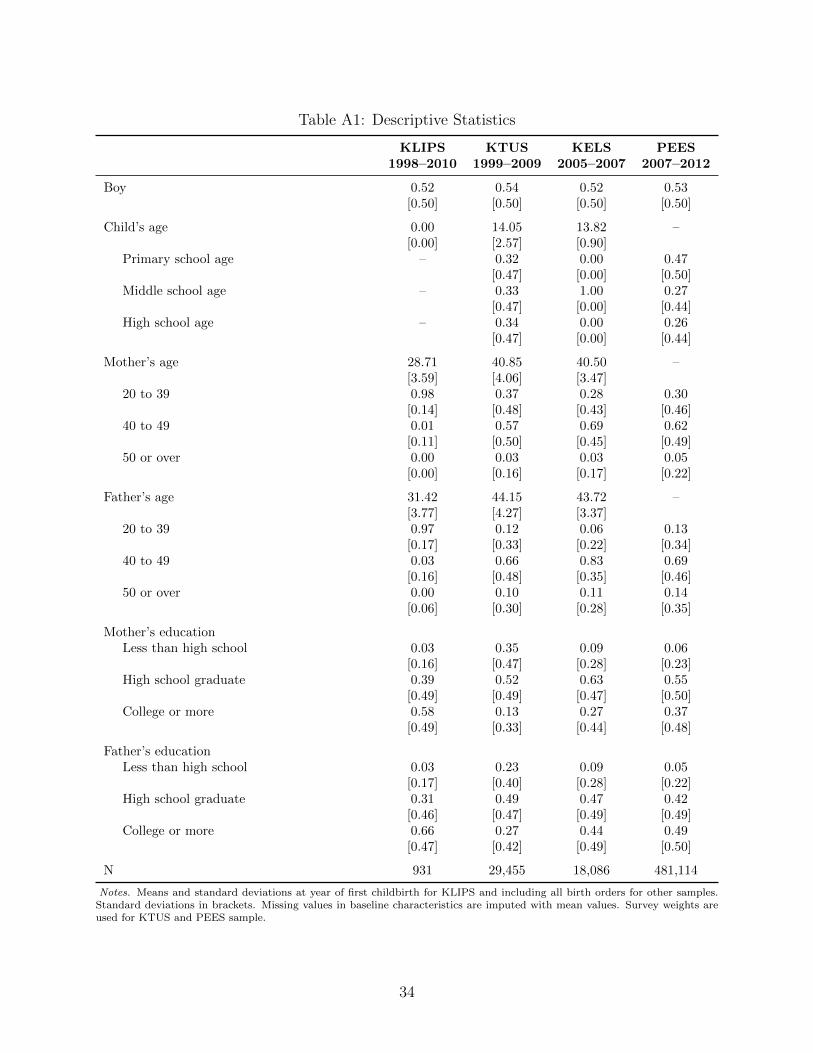
Table A1: Descriptive Statistics
KLIPS KTUS KELS PEES1998–2010 1999–2009 2005–2007 2007–2012
Boy 0.52 0.54 0.52 0.53[0.50] [0.50] [0.50] [0.50]
Child’s age 0.00 14.05 13.82 –[0.00] [2.57] [0.90]
Primary school age – 0.32 0.00 0.47[0.47] [0.00] [0.50]
Middle school age – 0.33 1.00 0.27[0.47] [0.00] [0.44]
High school age – 0.34 0.00 0.26[0.47] [0.00] [0.44]
Mother’s age 28.71 40.85 40.50 –[3.59] [4.06] [3.47]
20 to 39 0.98 0.37 0.28 0.30[0.14] [0.48] [0.43] [0.46]
40 to 49 0.01 0.57 0.69 0.62[0.11] [0.50] [0.45] [0.49]
50 or over 0.00 0.03 0.03 0.05[0.00] [0.16] [0.17] [0.22]
Father’s age 31.42 44.15 43.72 –[3.77] [4.27] [3.37]
20 to 39 0.97 0.12 0.06 0.13[0.17] [0.33] [0.22] [0.34]
40 to 49 0.03 0.66 0.83 0.69[0.16] [0.48] [0.35] [0.46]
50 or over 0.00 0.10 0.11 0.14[0.06] [0.30] [0.28] [0.35]
Mother’s educationLess than high school 0.03 0.35 0.09 0.06
[0.16] [0.47] [0.28] [0.23]High school graduate 0.39 0.52 0.63 0.55
[0.49] [0.49] [0.47] [0.50]College or more 0.58 0.13 0.27 0.37
[0.49] [0.33] [0.44] [0.48]
Father’s educationLess than high school 0.03 0.23 0.09 0.05
[0.17] [0.40] [0.28] [0.22]High school graduate 0.31 0.49 0.47 0.42
[0.46] [0.47] [0.49] [0.49]College or more 0.66 0.27 0.44 0.49
[0.47] [0.42] [0.49] [0.50]
N 931 29,455 18,086 481,114
Notes. Means and standard deviations at year of first childbirth for KLIPS and including all birth orders for other samples.Standard deviations in brackets. Missing values in baseline characteristics are imputed with mean values. Survey weights areused for KTUS and PEES sample.
34
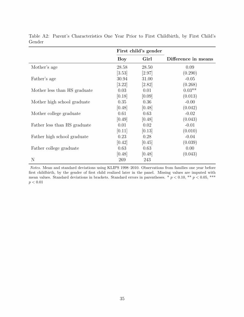
Table A2: Parent’s Characteristics One Year Prior to First Childbirth, by First Child’sGender
First child’s gender
Boy Girl Difference in means
Mother’s age 28.58 28.50 0.09[3.53] [2.97] (0.290)
Father’s age 30.94 31.00 -0.05[3.22] [2.82] (0.268)
Mother less than HS graduate 0.03 0.01 0.03**[0.18] [0.09] (0.013)
Mother high school graduate 0.35 0.36 -0.00[0.48] [0.48] (0.042)
Mother college graduate 0.61 0.63 -0.02[0.49] [0.48] (0.043)
Father less than HS graduate 0.01 0.02 -0.01[0.11] [0.13] (0.010)
Father high school graduate 0.23 0.28 -0.04[0.42] [0.45] (0.039)
Father college graduate 0.63 0.63 0.00[0.48] [0.48] (0.043)
N 269 243
Notes. Mean and standard deviations using KLIPS 1998–2010. Observations from families one year beforefirst childbirth, by the gender of first child realized later in the panel. Missing values are imputed withmean values. Standard deviations in brackets. Standard errors in parentheses. * p < 0.10, ** p < 0.05, ***p < 0.01
35

Table A3: Parent’s Characteristics, by Child’s Gender
First child’s gender
Boy Girl Difference in means
Mother’s age 40.88 40.81 0.07[4.15] [3.95] (0.060)
Father’s age 44.19 44.10 0.09[4.34] [4.20] (0.064)
Mother less than HS graduate 0.34 0.35 -0.00[0.47] [0.47] (0.007)
Mother high school graduate 0.53 0.52 0.01*[0.49] [0.49] (0.007)
Mother college graduate 0.13 0.14 -0.01*[0.32] [0.33] (0.005)
Father less than graduate 0.23 0.23 -0.00[0.40] [0.40] (0.006)
Father high school graduate 0.50 0.49 0.01[0.47] [0.47] (0.007)
Father college graduate 0.27 0.28 -0.01[0.42] [0.42] (0.006)
N 15,314 14,141
Notes. Mean and standard deviations using KTUS 1999–2009. Column (3) reports results from running sep-arate linear regressions where each characteristic is regressed on a dummy equal to 1 if child is male. Missingvalues are imputed with mean values. Standard deviations in brackets. Standard errors in parentheses. *p < 0.10, ** p < 0.05, *** p < 0.01
36
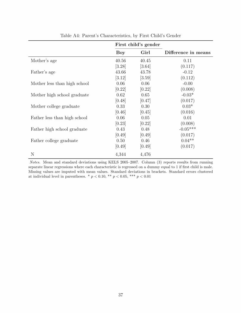
Table A4: Parent’s Characteristics, by First Child’s Gender
First child’s gender
Boy Girl Difference in means
Mother’s age 40.56 40.45 0.11[3.28] [3.64] (0.117)
Father’s age 43.66 43.78 -0.12[3.12] [3.59] (0.112)
Mother less than high school 0.06 0.06 -0.00[0.22] [0.22] (0.008)
Mother high school graduate 0.62 0.65 -0.03*[0.48] [0.47] (0.017)
Mother college graduate 0.33 0.30 0.03*[0.46] [0.45] (0.016)
Father less than high school 0.06 0.05 0.01[0.23] [0.22] (0.008)
Father high school graduate 0.43 0.48 -0.05***[0.49] [0.49] (0.017)
Father college graduate 0.50 0.46 0.04**[0.49] [0.49] (0.017)
N 4,344 4,476
Notes. Mean and standard deviations using KELS 2005–2007. Column (3) reports results from runningseparate linear regressions where each characteristic is regressed on a dummy equal to 1 if first child is male.Missing values are imputed with mean values. Standard deviations in brackets. Standard errors clusteredat individual level in parentheses. * p < 0.10, ** p < 0.05, *** p < 0.01
37
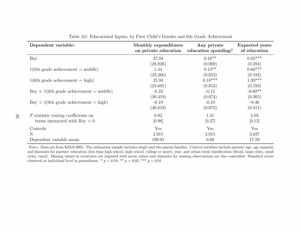
Table A5: Educational Inputs, by First Child’s Gender and 6th Grade Achievement
Dependent variable: Monthly expenditures Any private Expected yearson private education education spending? of education
Boy 27.04 0.16** 0.85***(28.826) (0.069) (0.284)
1(6th grade achievement = middle) 1.44 0.13** 0.60***(23.266) (0.053) (0.182)
1(6th grade achievement = high) 25.93 0.18*** 1.39***(23.691) (0.053) (0.193)
Boy × 1(6th grade achievement = middle) -6.23 -0.12 -0.60**(30.419) (0.074) (0.305)
Boy × 1(6th grade achievement = high) -6.19 -0.10 -0.46(30.819) (0.073) (0.311)
F -statistic testing coefficients on 0.02 1.31 2.03terms interacted with Boy = 0 [0.98] [0.27] [0.13]
Controls Yes Yes YesN 2,915 2,915 3,037Dependent variable mean 190.01 0.68 17.59
Notes. Data are from KELS 2005. The estimation sample includes single and two-parent families. Control variables include parents’ age, age squared,and dummies for parents’ education (less than high school, high school, college or more), year, and urban rural classification (Seoul, large cities, smallcities, rural). Missing values in covariates are imputed with mean values and dummies for missing observations are also controlled. Standard errorsclustered at individual level in parentheses. * p < 0.10, ** p < 0.05, *** p < 0.01
38