transitional water fish assemblage index of biotic ... · transitional water fish assemblage index...

Transitional Water Fish Assemblage Index of Biotic Integrity for

New Hampshire Wadeable Streams

January 2011

2

R-WD-11-6

Transitional Water Fish Assemblage Index of Biotic Integrity for

New Hampshire Wadeable Streams

New Hampshire Department of Environmental Services

PO Box 95

29 Hazen Drive

Concord, NH 03302-3503

(603) 271-8865

Thomas S. Burack

Commissioner

Michael J. Walls

Assistant Commissioner

Harry T. Stewart

Director

Water Division

Prepared By:

David E. Neils

Biological Program Manager

January 2011

3

TABLE OF CONTENTS

1. INTRODUCTION ………………………………………………………………….. 4

2. GENERAL PROCESS FOR TWIBI DEVELOPMENT ………………………… 5

3. METHODS ………………………………………………………………………….. 5

3.1 Identification of Expected Transitional Water Fish Assemblage Areas . 5

3.2 Comparison of Transitional and Strict Coldwater Assemblages ……… 6

3.3 Dataset ……………………………………………………………………… 6

3.4 Biological Response Indicators (metrics) ………………………………… 8

3.5 TWIBI scoring and threshold identification ……………………………. 10

3.6 Final Index Score Performance Evaluation ……………………………... 10

4. RESULTS ……………………………………………………………………………. 11

4.1 Transitional vs. Strict Coldwater Assemblages ………………………… 11

4.2 Transitional Water Fish Assemblage Area ……………………………… 15

4.3 Dataset Comparability ………………………………………………….... 16

4.4 Biological Response Indicators …………………………………………... 17

4.5 Metric and TWIBI Scoring ……………………………………………… 20

4.6 IBI Threshold Determination …………………………………………... 24

4.7 Validation Testing ………………………………………………………... 25

5. SUMMARY AND RECOMMENDATIONS ……………………………………… 28

6. REFERENCES ……………………………………………………………………... 32

7. APPENDICES ……………………………………………………………………… 34

A. Candidate metrics ……………………………………………………….. 34

B. Autecological fish characteristics …………………………………………… 36

C. Metric testing …………………………………………………………….. 37

D. Spearman correlation coefficients ………………………………………. 38

E. Stream names and sample locations …………………………………….. 39

4

1. INTRODUCTION

The following document describes the development of a transitional water fish assemblage Index of

Biotic Integrity (TWIBI) for New Hampshire wadeable streams. A transitional water fish

assemblage is meant to describe an assemblage that neither resides in a strict coldwater, nor

warmwater environment. Rather, transitional water fish assemblages reside in sections of rivers and

streams “transitioning” away from a coldwater assemblage (few species, dominated coldwater

specialists) and towards a warmwater assemblage (increased species richness, dominated by

warmwater generalists). As the name suggests, transitional water fish assemblages share the

biological attributes of two distinct fish assemblage types making them difficult to define with

absolute certainty, and therefore, subsequently locate a priori purely based on their physical

characteristics or geographic proximity.

The TWIBI is a numeric interpretation of the narrative water quality criteria as stated in New

Hampshire Department of Environmental Services Administrative Rules Env – Wq 1700 covered

under the statutory authority given in RSA 485-A:8, VI. Specifically, the narrative standard is

detailed in section 1703.19 as:

Env-Ws 1703.19 Biological and Aquatic Community Integrity.

(a) The surface waters shall support and maintain a balanced, integrated, and adaptive community of organisms having a species composition, diversity, and functional organization comparable to that of similar natural habitats of a region.

(b) Differences from naturally occurring conditions shall be limited to non-detrimental differences in community structure and function.

The product of the TWIBI development process detailed in this document will ultimately be used to

assess, in part, the health of applicable aquatic communities. Specifically, assessments under this

authority will be made for aquatic life use (ALU) determinations as required for 305(b)/303(d)

reporting to the United States Environmental Protection Agency (EPA). Additional applications

include, but are not limited to the establishment of permit limits, determination of non-point source

water quality impacts, water quality planning, and ecological risk assessment (Barbour et al. 1999).

As a two-part narrative criterion, the goal of index development was to first identify the natural

structure and function of the fish assemblages residing in the pertinent natural habitats [1703.19(a)],

and second, to determine when a detrimental departure from the natural condition has occurred

[1703.19(b)]. The basic approach taken for TWIBI development was the identification of a suitable

reference condition and establishment of a natural range of variation within this reference condition

(=identification of natural structure and function). Once identified, a reference condition threshold

was established below which the biological condition includes detrimental changes in overall aquatic

community structure and function (=departure from natural condition). Transitional water fish

assemblages not meeting or exceeding the reference condition threshold would be considered to

demonstrate significant unnatural community structure and function alterations and consequently not

attaining the narrative water quality standard in 1703.19 for ALU.

5

2. GENERAL PROCESS FOR TWIBI DEVELOPMENT

Indices of biological integrity for fish assemblages have been developed using a variety of

approaches over the past twenty years (Karr 1981; Leonard and Orth 1986; Lyons et al. 1996;

Mundahl and Simon 1999; Langdon 2001; Daniels et al. 2002; Hughes et al. 2004, and Whittier et

al. 2007). While these approaches differ in their objectivity, data analysis approaches, and final

index evaluation system, most follow the same basic developmental principles to arrive at a final

condition index to characterize the overall structure and function of the fish assemblage.

For New Hampshire, the process of developing a numeric index that interprets the biological

condition of transitional fish assemblages was similar to that described by Barbour et al. (1995) and

included five basic steps:

1) Reference sites selection: An a-priori process used to select sites with minimal human

impacts in order to establish the minimally impacted biological condition.

2) Transitional water fish assemblage identification: The determination of indicator species,

assemblage diversity, applicable area, and non-biological factors that describe this

assemblage type.

3) Identification of biological response indicators (metrics): The selection of the best

ecological measures of community structure and function. Generally known as metric

selection.

4) Establishment of index scoring criteria and thresholds: A comparison of reference and

non-reference biological conditions for the purpose of determining when substantial

unnatural impacts to ecological structure and function have occurred.

5) Validation of index: Testing of metric responses, comparison of reference and non-

reference conditions, and testing of the proposed threshold with an independent dataset.

The end result of the development process is a numeric index that includes multiple response

indicators (i.e. multi-metric) that are considered cumulatively to quantify the biological condition of

applicable streams. The index should be sensitive to human disturbance in that it demonstrates

declining biological conditions in response to increasing anthropogenic impacts.

3. METHODS

3.1 Identification of Expected Transitional Water Fish Assemblage Areas

In order to avoid the difficulties in defining a distinct set of physical or geographic characteristics for

rivers and streams that are expected to contain transitional water fish assemblages, areas supporting

this fish assemblage type were identified through a process of elimination. First, the identification

of the geographic boundaries of streams and rivers expected to support coldwater fish species year

round were delineated using predictions from a logistic regression model based on latitude,

longitude, and upstream drainage area (NHDES, 2007a). The areas not contained within these

predictions are expected to contain warmwater fish assemblages and will be analyzed at a later date.

6

Next, the applicable areas of the New Hampshire strict coldwater fish assemblage index of biotic

integrity (CWIBI) (NHDES, 2007b) were overlaid onto the expected coldwater fish species areas.

The resulting, non-overlapping area was deemed to best define streams and rivers that are expected

to contain transitional water fish assemblages (Map 1). Note, however, that by definition a

transitional water fish assemblage is expected to support coldwater fish species throughout the year.

Thus, transitional water fish assemblages were expected to resemble strict coldwater fish

assemblages, primarily by the presence of coldwater fish species, but with differences in species

richness and composition.

Map 1. Expected geographic distribution of 1

st – 4

th order streams expected to support coldwater fish species,

applicable CWIBI area, and areas expected to support transitional water fish assemblages.

3.2 Comparison of Transitional and Strict Coldwater Assemblages

After the geographic boundaries were defined, all sites falling within the area were included in

subsequent analyses. Once the final dataset was defined, the fish species composition and physical

characteristics (latitude, longitude, elevation, and drainage area) of the transitional water fish

assemblage reference sites were summarized and compared to reference sites included in the

previously developed CWIBI in order to determine the level similarity or uniqueness. Species

indicator analysis and non-metric multidimensional scaling (NMDS) were completed using PC-ORD

(MjM software, Version 4) as a final step to confirm the need for separate condition indices (IBIs).

3.3 Dataset

The development of a condition index for the transitional water fish assemblage included a total of

164 sites located in 1st to 4

th order rivers and streams. Data included in the development process

- =

A. Predicted area expected to support coldwater fish species

B. Applicable CWIBI area (strict coldwater fish assemblage)

C. Expected area of transitional water fish assemblages

A. B. C.

7

originated from sampling performed by the NHDES and the New Hampshire Fish and Game

Department (NHFGD). Of the original 164 sites, 29 were removed because fewer than 30

individuals were captured. The final dataset included 55 sites sampled by the NHDES from 1997 –

2007. At each site a representative sample reach of 150 meters was delineated and fish were

collected in a single pass backpack electrofishing effort. All sites were part of the annual biological

monitoring sampling program. For the NHFGD, data from two distinct programs was included.

First, 43 sites were sampled as part the NHFGD’s inland fisheries summer assessment program

(SAP). These sites generally included a 100 – 150 meter sampling reach with fish collected during a

single or multiple pass backpack electrofishing effort. Thirty-seven additional sites were included

from NHFGD’s Fishing-for-the-Future program (FFF). A similar sampling effort was employed for

these sites with site selection focused on rivers and streams that had been previously stocked with

coldwater gamefish species. Fieldwork for each of the programs above was completed primarily

from 1995 – 2007.

The dataset was randomly broken into calibration and validation subsets. The calibration dataset

included 31 reference sites, 27 minimally impacted sites, 31 moderately impacted sites, and 10

impacted (high) sites (Table 1). The validation dataset was designed to test the performance of the

index and consisted of 11 reference, 9 minimally impacted, 10 moderately impacted, and 6 impacted

sites. Reference sites were defined as “minimally disturbed” (Stoddard et al. 2006). Reference site

identification and narrative impact ratings were based on the activities within the upstream drainage

area and determined from a combination of a quantitative human disturbance rating system for the

NHDES sites and aerial / topographic map inspection for NHFGD sites. Reference site

determinations and impact ratings for NHFGD sites were finalized by the respective agency

biologists familiar with the sample locations and their contributing drainage area.

Table 1. Number of sites in the calibration and validation datasets sampled by NHDES and NHFGD.

Level of Impact

Agency Project Reference Minimum Moderate High Totals

CALIBRATION

NHDES Annual Sampling 9 15 12 4 40

Annual Sampling (SAP) 14 6 9 4 33 NH Fish and Game

(NHFGD) Fishing for the Future (FFF) 8 6 10 2 26

Totals 31 27 31 10 99

VALIDATION

NHDES Annual Sampling 4 3 6 2 15

Annual Sampling (SAP) 2 6 0 2 10 NH Fish and Game

(NHFGD) Fishing for the Future (FFF) 5 0 4 2 11

Totals 11 9 10 6 36

For all sites as many fish as possible were collected during active sampling. After sampling was

complete all fish were identified, enumerated, recorded, and immediately returned to the river or

stream from which they were collected. Length and weight data were also collected for gamefish

8

species for all NHFGD sites. For all sites, inclusion into the index development process required

that each species had a minimum of two individuals. In addition, Atlantic salmon were excluded

from the dataset since they only exist in New Hampshire rivers and streams through stocking efforts.

Finally, because salmonid fish species represent an integral component of any fish assemblage from

which they are expected to occur, their origin and life stage are important to characterize when

making condition assessments. While many of the sampling stations included in the dataset were

known to contain both wild and stocked individuals, their origin was not always available from the

data. Therefore, since wild salmonids in New Hampshire tend to be smaller than hatchery raised

fish, a size limit was imposed to differentiate their origin where information was otherwise lacking.

Based on input from NHFGD biologists, all salmonid individuals less than 180mm were considered

wild (naturally produced) and subsequently retained for further analysis. In contrast, salmonid

individuals greater than 180mm were assumed to be hatchery raised and excluded from further

analysis. While, on occasion, wild salmonids certainly exceed 180mm in length in NH; such large,

wild individuals are relatively uncommon.

With regards to life stage [young-of-year (YOY) or adult], where information was not available, a

90mm length threshold was established by the NHFGD whereby individuals less than 90mm were

designated as YOY. Individuals exceeding 90mm in length were designated as adults.

Once final datasets were adjusted as described above, species richness, rank species abundance, and

the number of individuals captured per site was compared between NHDES and NHFGD sites to

ensure that the data sources were compatible. Kruskal-Wallis and Mann-Whitney U tests were used

to determine if differences were detectable in environmental characteristics between the datasets.

3.4 Biological Response Indicators (Metrics)

Candidate metrics were selected from previously developed fish indices (Hughes et al. 2004; Karr

1981; Langdon 2001; Leonard and Orth 1986; Lyons et al. 1996; Mundahl and Simon 1999; Daniels

et al. 2002; Whittier et al. 2007) and tested for their ability to respond to varying levels of human

disturbance. Candidate metrics were classified into 8 major groups that included trophic class,

tolerance to pollution, thermal preference, streamflow preference, species richness, reproductive

strategy and success, assemblage composition, and origin (native or introduced) (Appendix A). For

each metric, an expected response to impact was noted and used in the metric testing process.

Expected responses were either positive (i.e. higher for reference than impacted sites) or negative

(lower for reference than impacted sites). Species common names, scientific names and the

respective ecological, pollution tolerances, thermal preferences, reproductive strategies, and origin

for the most commonly encountered species are presented in Table 2.

9

Table 2. Names, abbreviations, origin, and autecological characteristics of fish species most commonly encountered at

transitional water fish assemblage sampling locations. See Appendix B for explanation of abbreviations.

Common name

Scientific name

Abbreviation Origin Tolerance Trophic class

Thermal preference

Reproductive Strategy1

Streamflow preference2

Streamflow preference3

Blacknose dace

Rhinichthys atratulus BND N T OI ET S_L r fs

Brook trout

Salvelinus fontinalis EBT N I TC CW S_L r fs

Brown trout Salmo trutta BT I I TC CW S_L r fs

Burbot Lota lota BRB N M TC CW S_L x mg

Creek chub

Semotilus atromaculatis CC N T GF ET S_L x fs

Common shiner

Luxilus cornutus CS N M GF ET S_L x fd

Fallfish Semotilus corporalis FF N M GF ET S_L x fs

Lake chub Couesius plumbeus LC N M GF CW S_L mg

Longnose dace

Rhinichthys cataractae LND N M BI ET S_L r fs

Longnose sucker

Catostomus catostomus LNS N M BI CW S_L x fd

Rainbow trout

Oncorhynchus mykiss RT I I TC CW S_L r fs

Slimy sculpin

Cottus cognatus SS N I BI CW H_D r fs

Spottail shiner

Notropis hudsonius STS I M OI WW S_L l mg

White sucker

Catostomus commersoni CWS N T GF ET S_L x fd

from 1 - Simon 1999; based on Balon 1975; 2 - from Stoddard et al. 2007; 3 - from Bain 1996

In order to determine the appropriateness of a candidate metric’s inclusion into the final index a

multi-step process was implemented that first included examining the distribution of metric values

for reference and impacted sites. For each metric, reference and impacted site distributions were

compared by first computing the 25th

and 75th

percentiles for reference sites and then determining

the percentage of impacted site values that fell within the reference range. If greater than 60 percent

of the impacted site values fell within the reference range the metric was eliminated (Sensu Whittier

et al. 2007). Next, mean reference and impacted site metric values were compared and matched

with the expected responses for individual metrics. Metrics that displayed observed responses

counter to expected responses were also eliminated.

After the initial metric testing phase, all remaining metrics were evaluated with respect to natural

environmental gradients to determine if any significant relationships were apparent. The objective

of this step was to account for natural variation in metric values that was unrelated to the stressor

gradient. To accomplish this, metric values from reference sites were regressed against

environmental variables. For each candidate metric and environmental variable combination,

regression significance was computed, data plots examined, and 75 percent prediction interval lines

constructed to determine if a strong relationship existed.

10

The third phase of candidate metric testing included a detailed objective comparison between

reference and test site distributions. First, significant differences between reference and impacted

sites were determined from Mann-Whitney U tests for all metrics. The absolute value of the Z-

scores for the respective candidate metrics were ranked from highest to lowest for each major metric

category with the presumption that higher Z-scores indicated a more distinct stressor response

(Whittier et al. 2007). Next, the mean, median, 75th

, and 25th

percentiles were computed for each

metric and compared in five combinations (See appendix C). The total number and magnitude of

correct responses for each metric was examined. These results were paired with the significance

testing to arrive at an initial list of final metrics.

Once the final list of potential metrics was determined, redundancy testing was performed using the

Spearman correlation coefficient. A target maximum correlation coefficient of 0.75 was established

whereby metrics with coefficients greater than this value were considered excessively redundant

requiring the selection of one or the other. In a limited number of cases some leniency was allowed

in applying this rule in order to further consider candidate metrics for inclusion into the final index.

The final step in the metric testing phase included a review of the results from the steps outlined

above. In some cases, similar metrics were interchanged in an attempt to balance the final index

with regards to the number of positive and negative response metrics, major metric categories, and

important fish assemblage characteristics. Final metric selection was designed to minimize metric

redundancy, maximize the selection of metrics with the greatest separation between reference and

impacted sites, and the inclusion of metric types that captured broad structural and functional

ecological categories. Cumulative frequency distributions and box and whisker plots were

constructed as a final visual aid in comparisons between reference and impacted sites for the

selected metrics.

3.5 TWIBI scoring and threshold identification

Scores for individual metrics were established by reviewing the frequency distribution of reference

and impacted sites. Specifically, three scoring categories (1, 3, and 5) were established to be

consistent with previously developed fish indices by the Vermont Department of Environmental

Conservation (VTDEC) (VTDEC 2004) with higher scores representing better condition. Then, for

each metric, raw values for reference sites were examined using cumulative frequency distributions

and the 25th

(positive response metrics) or 75th

(negative response metrics) percentiles in order to

assign logical breakpoints for the metric scoring categories. Once categorical scoring thresholds

were determined, scores were assigned to individual metrics for each site and a final index score

computed by summing individual metric scores. A final TWIBI threshold for aquatic life use

attainment was based on the 25th

percentile index score for reference sites.

3.6 Final Index Score Performance Evaluation

As a final check on the ability of the index to discriminate along a human disturbance gradient, a

Kruskal-Wallis test was completed for index scores across impact categories followed by Mann-

Whintey U tests for pair-wise impact category comparisons. Finally, based on the recommended

aquatic life use threshold, the number of sites meeting and failing to meet this threshold was

determined for each site type. Contingency tables based on these outcomes were compared (Chi-

11

square) for reference and test sites to determine if the distribution of sites exceeding and failing to

meet the recommended criteria were significantly different from random expectations.

4. RESULTS

4.1 Transitional vs. Strict Coldwater Assemblages

The expected species composition and abundance of sites used in the development of the TWIBI

was based on 31 reference sites from the calibration dataset and included 3,318 individuals from 14

species. Overall, blacknose dace was the most commonly collected species (87% of sites), followed

by brook trout (77%), longnose dace (65%), longnose sucker (58%), and slimy sculpin (58%) (Table

3). The same suite of species also had the highest overall relative abundance [blacknose dace (25%

of individuals), longnose dace (23%), slimy sculpin (17%), brook trout (8%), longnose sucker (8%)].

Table 3. Frequency of occurrence, total number of individuals, and rank abundance of fish species collected at

transitional water fish assemblage reference sites. Rank of ranks is inverse ranking of sum of ranks for # sites

present, percent of all individuals, average percent individuals/site.

Species # Sites Present

of Sites Present

Rank Total

Number Individuals

% of All Individuals

Rank Average %

Individuals / Site

Rank Sum of

Rank

Rank of Ranks

BND 27 87.1 1 845 25.3 1 31.3 3 5 1

BRB 6 19.4 8 36 1.1 10 6.0 13 31 10

BT 3 9.7 10 28 0.8 11 9.3 11 32 12

CC 2 6.5 12 28 0.8 11 14.0 8 31 10

CS 2 6.5 12 27 0.8 13 13.5 9 34 13

CWS 8 25.8 6 50 1.5 9 6.3 12 27 9

EBT 24 77.4 2 282 8.4 4 11.8 10 16 4

FF 3 9.7 10 51 1.5 8 17.0 5 23 8

LC 5 16.1 9 234 7.0 6 46.8 1 16 4

LND 20 64.5 3 783 23.4 2 39.2 2 7 2

LNS 18 58.1 4 277 8.3 5 15.4 7 16 4

RT 7 22.6 7 114 3.4 7 16.3 6 20 7

SS 18 58.1 4 563 16.8 3 31.3 4 11 3

STS 2 6.5 12 11 0.3 14 5.5 14 40 14

In comparison, the development of the CWIBI from 33 reference sites included 3,008 individuals

from 10 species (NHDES, 2007a). The five species with the highest relative frequency, in

decreasing order, from CWIBI reference sites was brook trout (94% of sites), slimy sculpin (76%),

blacknose dace (37%), longnose dace (24%), and rainbow trout (12%) (Table 4). The overall

relative abundance of these same species ranked highest among the CWIBI reference sites and were

as follows: brook trout (33%), blacknose dace (31%), slimy sculpin (25%), longnose dace (4%), and

rainbow trout (2%).

12

Table 4. Frequency of occurrence, total number of individuals, and rank abundance of fish species collected at

coldwater fish assemblage sites. See Table 2 for explanation of “Rank of Ranks”.

Species # Sites Present

% of Sites

Present Rank

Total Number

Individuals

% of All Individuals

Rank Average %

Individuals / Site

Rank Sum of Ranks

Rank of Ranks

BND 12 36.6 3 934 31.1 2 15.4 3 8 3

BT 2 6.1 9 18 .6 8 .5 8 25 9

CWS 3 9.1 6 35 1.2 7 .8 7 30 7

CC 2 6.1 9 7 .2 10 .4 10 29 10

EBT 31 93.9 1 1006 33.4 1 49.9 1 3 1

LC 33 9.1 6 55 1.8 6 2.3 6 18 6

LND 8 24.2 4 125 4.2 4 3.4 4 12 4

LNS 3 9.1 6 17 .6 9 .5 9 24 8

RT 4 12.1 5 64 2.1 5 2.8 5 15 5

SS 25 75.8 2 747 24.8 3 24 2 7 2

As suspected, reference sites for strict coldwater and transitional water fish assemblages shared

similar overall species compositions. NMDS analysis of these assemblage types using species

presence / absence data confirmed this finding (Figure 1). A general lack of site-grouping by

category (fish assemblage type) is indicative of biological communities that share the same species

compositions.

Figure 1. Nonmetric multidimeninal squaring ordination (NMDS) plot of cold- and transitional water fish assemblage

reference site based on fish species presence absence. Final stress = 17.8; instability = 0.005. Open triangles

(1) = coldwater reference sites; closed triangles (2) = transitional water reference sites.

13

While similarities were apparent among these assemblage types based solely on species presence or

absence, significant differences in species richness (Mann-Whitney U; Z-score = -4.02, p<0.0001)

were detected with transitional fish assemblages having more species (4.6) on average than strict

coldwater assemblages (2.8) (Figure 2). When the relative frequencies and abundances of individual

species were examined more closely, clear differences in transitional and strict coldwater

assemblages were obvious. For example, while blacknose dace was regularly encountered at

reference sites from both assemblage types, its relative frequency (percentage of species occurrences

within each fish assemblage type) was much higher for transitional fish assemblage sites (87%) than

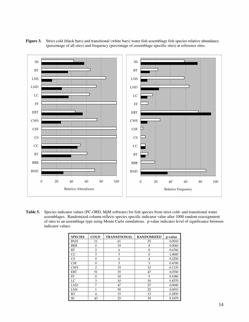
coldwater fish assemblage sites (36%) (Figure 3). Additional species which were more frequently

encountered at one assemblage type than another were longnose sucker, longnose dace, burbot, and

white sucker. In addition, several species were exclusive to, or had higher relative abundances

(percentage of species occurrences across assemblage types) in transitional than coldwater fish

assemblage sites (Figure 3). Fallfish, pumpkinseed, common shiner, and burbot were all found only

at transitional assemblage sites. Longnose sucker, longnose dace, white sucker, and blacknose dace

all occurred in higher relative abundances at transitional than coldwater assemblage sites.

Figure 2. Number of fish species at cold- and transitional water reference sites.

0

2

4

6

8

10

12

1 2 3 4 5 6 7 8 9

Number of Species

Fre

quency

Strict Coldwater

Transitional

Relative frequencies and abundances were combined to compute species indicator values (PC-ORD,

MjM software). Higher indicator values are indicative of species with a strong membership to a

particular assemblage type. For the transitional fish assemblage type, the species that served as the

best indicators were blacknose dace, longnose sucker, longnose dace, and burbot. Each of these

species had the highest indicator value differences among transitional and strict coldwater

assemblage types and were also significantly different from indicator values produced from

randomized data (Table 5).

14

Figure 3. Strict cold (black bars) and transitional (white bars) water fish assemblage fish species relative abundance

(percentage of all sites) and frequency (percentage of assemblage-specific sites) at reference sites.

Table 5. Species indicator values (PC-ORD, MjM software) for fish species from strict cold- and transitional water

assemblages. Randomized column reflects species specific indicator value after 1000 random reassignment

of sites to an assemblage type using Monte Carlo simulations. p-value indicates level of significance between

indicator values.

SPECIES COLD TRANSITIONAL RANDOMIZED p-value

BND 11 61 35 0.0010

BRB 0 19 8 0.0060

BT 2 6 8 0.6760

CC 3 3 6 1.0000

CS 0 6 4 0.2250

CSF 0 3 3 0.4700

CWS 2 19 13 0.1170

EBT 51 35 47 0.0700

FF 0 10 5 0.1080

LC 3 10 10 0.4570

LND 7 47 27 0.0040

LNS 1 50 22 0.0010

RT 4 15 13 0.2850

SS 43 25 39 0.1870

0 20 40 60 80 100

BND

BRB

BT

CC

CS

CSF

CWS

EBT

FF

LC

LND

LNS

RT

SS

Relative Abundance

0 20 40 60 80 100

BND

BRB

BT

CC

CS

CSF

CWS

EBT

FF

LC

LND

LNS

RT

SS

Relative Frequency

15

The environmental characteristics also differed when transitional and strict coldwater fish

assemblage reference sites were compared. Upstream drainage area had the most significant

difference between transitional and strict coldwater assemblage reference sites with mean drainage

areas of 31 and 7 square miles, respectively (Mann-Whitney U test; Z-score = -5.64; p<0.0001)

(Table 6). In addition, reference sites from transitional waters tended to be more northerly (Mann-

Whitney; Z-score = -2.35; p=0.019) and westerly (Mann-Whitney U test; Z-score = -2.08; p=0.037)

than from strict coldwaters. Elevation did not differ significantly between transitional and strict

coldwater reference sites.

Table 6. Latitude (dd.dddd), longitude (dd.dddd), elevation (ft), and drainage area (sq. mi.) of reference sites for strict

cold (CW) and transitional (TW) water fish assemblages. Asterisk indicates Mann-Whitney U test

significantly different at p<0.05.

Fish Assemblage Type

N Mean Std. Error of Mean

Median Minimum Maximum

Latitude*

CW 33 44.2071 0.10 44.3266 42.7313 45.1941

TW 31 44.5107 0.09 44.5317 43.3552 45.1084

Longitude*

CW 33 71.4663 0.07 71.3699 71.0246 72.4281

TW 31 71.2747 0.03 71.2306 71.0351 71.7919

Area*

CW 33 7.1 0.72 6.7 0.2 13.6

TW 31 31.3 2.85 34.7 3.7 63.5

Elevation

CW 33 1157 73.14 1180 337 1999

TW 31 1063 65.40 1157 439 1658

4.2 Transitional Water Fish Assemblage Area

The area identified as expected to contain transitional water fish assemblages and subsequently

applicable to the TWIBI was 1,622 square miles (Map 2). In total, the area represents 17.5% of the

State of New Hampshire. The applicable TWIBI area is primarily located in central and northern

sections of state with scattered areas along the western border of New Hampshire. The area

identified in Map 2 is meant to serve as general guidance for determining when the TWIBI should

be applied. However, for any given site, measures of latitude, longitude, and upstream drainage area

will serve as the primary determinants in conjunction with the rules outlined in Section 3.1 when

deciding if the TWIBI is the most appropriate fish index to assess the biological condition of the fish

assemblage.

16

Map 2. Expected areas of transitional water fish assemblage occurrence and respective index of biological integrity

(IBI) application.

4.3 Dataset Comparability

Prior to the index calibration phase, data source compatibility testing demonstrated a high level of

similarity between data collected by the NHDES and the NHFGD. Mean species richness across all

impact categories was not significantly different for sites sampled by the NHDES (4.4), the FFF

Applicable TWIBI area

White Mountain National Forest

boundaries

Major rivers and streams

17

(5.2), and the SAP (5.1) (Kruskal-Wallis, p=0.67). Species composition was also similar with the

three calibration data sources sharing the same top four species in terms of their rank abundance

(Table 7). Overall, for each data source, blacknose dace was the most abundant species and

comprised between 28 and 37 percent of all individuals collected. For the FFF dataset, slimy sculpin

(14%) and longnose dace (13%) were the next most abundant species. For the SAP dataset,

longnose dace (13%) and fallfish (11%) were the next most abundant species. The relative

abundances of the top three species for each respective dataset accounted for between 55 to 67

percent of the individuals captured.

Table 7. Relative abundance and rank of species for sites sampled by the New Hampshire Department of

Environmental Services (DES) and two programs (SAP, FFF) by the New Hampshire Fish and Game

Department (NHFGD).

DES NHFGD SAP NHFGD FFF Species

Individuals Percent Rank Individuals Percent Rank Individuals Percent Rank

BND 2127 36.9% 1 1903 31.8% 1 1123 28.1% 1

BRB 89 1.5% 10 57 1.0% 13 57 1.4% 13

BT 19 0.3% 14 40 0.7% 14 11 0.3% 14

CC 26 0.5% 12 109 1.8% 11 128 3.2% 9

CS 254 4.4% 5 492 8.2% 5 224 5.6% 7

CWS 203 3.5% 7 227 3.8% 8 286 7.2% 5

EBT 484 8.4% 4 249 4.2% 7 300 7.5% 4

FF 250 4.3% 6 665 11.1% 3 264 6.6% 6

LC 130 2.3% 8 178 3.0% 9 76 1.9% 11

LND 1153 20.0% 2 795 13.3% 2 517 12.9% 3

LNS 124 2.2% 9 596 10.0% 4 129 3.2% 8

RT 34 0.6% 11 82 1.4% 12 126 3.2% 10

SS 552 9.6% 3 354 5.9% 6 575 14.4% 2

STS 26 0.5% 12 132 2.2% 10 76 1.9% 11

The mean total number of individuals collected per sampling event was significantly different

among the data sources with mean abundances of 105, 162, and 99 individuals at DES, FFF, and

SAP sites, respectively (Kruskal-Wallis, p=0.036). However, since the index development process

did not include absolute abundance metrics in the calibration phase (see section 4.4 below), the

significant differences that were observed were not considered to be problematic. The similarity in

site species richness and composition were considered adequate for combining the data sources in all

subsequent aspects of index development.

4.4 Biological Response Indicators

The performance of 72 candidate metrics was tested using the calibration dataset to determine those

best suited to describe the condition of a transitional water fish assemblage. Of these, 28 (38.9%)

had both a sufficient non-overlapping range (< 60 percent of impacted sites contained within the 25th

and 75th

percentiles of the reference distribution) and the correct expected response when reference

and impacted sites were compared (Table 8). Metrics that displayed substantial overlapping ranges

18

between reference and impacted sites or a did not have the correct stressor response were excluded

from further consideration. Of the eight major metric categories, the richness, reproductive, and

non-native groups failed to produce at least one metric to be carried forward into to subsequent

phases of metric testing.

Table 8. Number of candidate metrics in each major category and number retained for additional testing.

Metric Category # Candidate

metrics

# Retained for

testing %

Non-native 4 0 0.0

Composition / Indicator taxa 18 7 38.9

Reproduction 4 0 0.0

Trophic 8 3 37.5

Richness 2 0 0.0

Streamflow preference 17 4 23.5

Thermal preference 9 6 66.7

Tolerance 10 8 80.0

TOTAL 72 28 38.9

Possible relationships between metrics and natural environmental gradients were investigated for the

remaining 28 metrics. The environmental variables included latitude, longitude, elevation, drainage

area. Overall, a total of 12 significant (p<0.05) linear regressions were detected between individual

metrics and environmental variables out of 112 combinations (28 metrics x 4 environmental

variables). The remaining 28 candidate metrics were most frequently related to a site’s elevation

and latitude (4 each) as compared to other potential environmental gradients – area (3) and longitude

(1). Of the 12 instances where significant metric-environmental variable relationships were

detected, the highest observed R2 value was 0.39 indicating that less than 50 percent of the variation

was explained by the environmental variable. Further, in all cases where significant regressions

were detected, the 75 percent prediction intervals for the minimum and maximum metric value

demonstrated substantial overlap. Thus, it was concluded that none of the metrics required

adjustment to take into account natural influences by environmental variables.

Twenty-four of the remaining 28 candidate metrics (86 percent) indicated either significantly higher

(positive-response metrics) or lower (negative-response metrics) metric values for reference sites

when reference and impacted sites were compared (Mann-Whitney U Test; p<0.05) (Table 9).

Metrics that did not have significantly different responses (Mann-Whitney U Test p>0.05) between

reference and impacted sites were excluded from further consideration into the index. Significant

Mann-Whitney U tests were coupled with four separate measures of the magnitude of separation

between metric values for reference and impacted sites (Appendix C). A decision was made to carry

forward those metrics with the highest ranking based on the Mann-Whitney U test Z-scores and / or

the greatest number of correct responses based on the degree separation between reference and

impacted sites within each of the metric groups. For the thermal and tolerance metric groups an

additional metric was retained for redundancy testing because these groups had the greatest number

of metrics pass the first phase of testing (Table 8).

In all twelve metrics were selected for further consideration; eight were positive response metrics

and four were negative response metrics (Table 9). Each metric, except for the per_T_sp and

ct_CW_sp metrics, either ranked first or second in its respective metric group based on the Mann-

19

Whitney U test or had four or more correct test responses. The per_T_sp metric was retained

because it was the best performing negative response metric in the tolerance metric group that

regularly occurred at both reference and impacted sites in relative abundances greater than 20

eprcent (Table 8). Metric redundancy proved to be minimal with only three of the sixty-six possible

metric combinations having inter-metric Spearman correlation coefficients in excess of 0.75

(Appendix D). However, of the three candidate metrics selected within the thermal category, the

per_CW_sp and per_CW metrics were near the correlation coefficient threshold with the per_T_sp

(-0.72) and EBT_SS (0.72), respectively. For this reason, the ct_CW_sp metric was considered to

be the best representative from the thermal category as it had much lower correlation coefficients

with the eleven other candidate metrics.

Table 9. Results of candidate metric testing between reference and impacted sites. Rank = Mann-Whitney U test Z-

score rank within major metric category. # Correct responses = result of Mann-Whitney U test, mean,

median, percentile testing (see appendix C). Bolded metrics carried forward through redundancy testing.

Mann-Whitney U Test

METRIC Type Expected response

Mean (reference)

Mean (impacted) Significance

Z-score

Rank # Correct Responses

BND composition - 25.5 29.0 0.277 N/A N/A 1

CS composition - 0.7 5.7 <0.001 -4.39 2 2

CWS composition - 1.6 9.2 0.003 -2.99 5 2

CC_CS_FF composition - 2.6 18.7 <0.001 -4.35 3 4

CC_CS_FF_BND composition - 28.1 47.7 <0.001 -3.50 4 2

EBT composition + 11.7 2.5 0.004 -2.86 6 4

EBT_SS composition + 29.2 6.4 <0.001 -4.50 1 5

per_no_lotic streamflow - 4.1 5.7 0.113 N/A N/A 2

per_r streamflow + 80.6 48.6 <0.001 -3.53 2 4

per_r_x streamflow + 95.9 94.3 0.113 N/A N/A 2

per_fs_ex_bnd streamflow + 57.0 34.8 <0.001 -3.82 1 3

per_et thermal - 51.8 74.6 0.001 -3.25 6 2

ct_et_sp thermal - 2.1 4.2 <0.001 -3.88 3 5

per_et_sp thermal - 43.5 71.5 <0.001 -3.79 4 3

per_CW thermal + 47.8 17.3 <0.001 -3.90 2 4

ct_CW_sp thermal + 2.6 1.1 <0.001 -3.57 5 5

per_cw_sp thermal + 54.9 18.8 <0.001 -4.44 1 5

per_M tolerance - 38.3 51.4 0.262 N/A N/A 2

per_T tolerance - 28.1 41.7 0.016 -2.42 7 2

per_tol_GF tolerance - 2.6 12.7 <0.001 -3.68 2 5

per_M_sp tolerance - 39.0 49.0 0.011 -2.53 6 4

per_T_sp tolerance - 25.7 38.9 0.004 -2.91 5 3

per_I tolerance + 33.6 6.9 <0.001 -4.55 1 5

ct_I_sp tolerance + 1.7 0.7 0.001 -3.38 4 4

per_I_sp tolerance + 35.3 12.1 <0.001 -3.57 3 4

per_GF trophic - 8.5 31.2 <0.001 -4.18 1 5

ct_GF_sp trophic - 0.7 2.2 <0.001 -3.91 2 5

per_BI trophic + 48.3 26.2 <0.001 -3.65 3 4

20

Metrics with the most separation between reference and impacted sites as well as a low level of

redundancy were selected for inclusion in the index. Metric selection was also based on the

inclusion of as many of the major metric categories as possible in order to reflect a transitional water

fish assemblage with a balanced, integrated, and adaptive aquatic community structure and

composition.

With these requirements in mind, a set of seven metrics was selected for inclusion into the index

(Table 10). All seven metrics had significantly different values between reference and impacted

sites (Mann-Whitney U test) and displayed three or more out of five correct performance responses.

An eighth metric was added to reflect the age class structure of book trout. While not tested

concurrently with the candidate metrics, a decision was made to include at least one metric that

reflected the reproductive success of an important indicator species of the transitional water fish

assemblage. As a final check on the degree of separation between reference and impacted sites, box

plots were constructed for the metrics selected for inclusion into the TWIBI (Figure 4).

Table 10. Final metrics, abbreviations, and metric category selected for inclusion into the TWIBI. Mean, minimum,

and maximum for reference (n=31) and impacted sites (n=10) for the calibration dataset.

Reference Impacted

Metric Abbreviation Category mean min max mean min max

Percentage of Book trout and slimy sculpin

EBT_SS Composition /Indicator taxa

29.2 0.0 100.0 6.4 0 50.0

Percentage of creek chub, common shiner, and fall fish

CC_CS_FF Composition /Indicator taxa

2.6 0.0 33.0 18.7 0 53.5

Percentage of fluvial specialists excluding blacknose dace

per_fs_ex_bnd Composition /Indicator taxa

57.0 2.6 100.0 34.8 9.7 89.1

Number of coldwater species

ct_CW_sp Thermal preference

2.6 0.0 5.0 1.1 0.0 4.0

Percentage of tolerant species

per_T_sp Tolerance 25.7 0.0 50.0 38.9 12.5 50.0

Percentage of benthic insectivores

per_BI Trophic 48.4 0.0 83.5 26.2 0 58.9

Percentage of generalist feeders

per_GF Trophic 8.5 0 41.5 31.2 7.7 66.2

Brook trout class age structure

EBT_age_class Reproduction ----- ----- ----- ----- ----- -----

4.5 Metric and TWIBI scoring

Raw metric values were converted to a numeric score based on the IBI schema established by the

VT DEC (VTDEC 2004). Each metric from an individual site was eligible for one of three scoring

categories (1, 3, 5) depending on the raw metric result. Low metric scores were used to reflect

poorer assemblage condition. Metric score categories and corresponding raw metric thresholds were

established by examining the cumulative frequency distributions of reference and impacted sites.

For all metrics, a clear separation between reference and impacted sites was observed (Figure 5).

Natural breakpoints in line slope for either reference or impacted cumulative frequency distributions

were useful as an investigatory tool in identifying proposed scoring thresholds for most metrics.

21

Figure 4. Box and whisker plots of TWIBI metrics for reference and impacted sites from the calibration dataset. Upper

extent of box is 75th

percentile. Lower extent of box is 25th

percentile. Line inside box is median. Upper whisker = [1.5

x (75th

– 25th

percentile]+ 75th

percentile. Lower whisker = [1.5 x (75th

– 25th

percentile] – 25th

percentile. Circles (�)

indicate outlier points (1.5-3x interquartile range).

IMPREF

100

80

60

40

20

0

% In

div

idu

als

EBT_SS

IMPREF

100

80

60

40

20

0%

In

div

idu

als

CC_CS_FF

IMPREF

100

80

60

40

20

0

% In

div

idu

als

per_BI

IMPREF

70

60

50

40

30

20

10

0

% In

div

idu

als

per_GF

IMPREF

100

80

60

40

20

0

% In

div

idu

als

per_T_sp

IMPREF

100

80

60

40

20

0

% In

div

idu

als

per_FS_ex_bnd

IMPREF

4

2

0

Nu

mb

er

Sp

ec

ies

ct_CW_sp

22

Figure 5. Cumulative frequency distributions of reference (grey lines) and impacted (black lines) sites from the

calibration dataset and proposed scoring cutpoints. Long dashes = cut between 3 and 5 points. Short intermittent dashes

= cut between 1 and 3 points.

For all metrics, a high percent of reference sites fell within the highest scoring category. For

example, 65 percent of reference sites were within the highest scoring category for the percentage of

benthic insectivore metric (per_BI), a positive response metric (Table 11). Conversely for the

percentage of generalist feeders metric (per_GF metric), only 13 percent of reference sites were

contained within the lowest scoring category. An attempt was made to include greater than 50

percent of reference sites and less than 20 percent of impacted sites in the highest scoring category.

Logically, the proposed scoring thresholds generally also resulted in a much higher percentage of

impacted sites in the lowest scoring category as compared to reference sites. The proposed scoring

thresholds for each metric (Table 11) were designed to account for the raw analytical differences in

the distribution of reference and impacted site data and reflect the associated structural and

compositional responses of a transitional water fish assemblage to stressors.

ct_CW_sp

0%

20%

40%

60%

80%

100%

0 1 2 3 4 5 6

Number of species

Percent of Sites

per_BI

0%

20%

40%

60%

80%

100%

0% 20% 40% 60% 80% 100%

Percent Individuals

Percent of Sites

per_GF

0%

20%

40%

60%

80%

100%

0% 20% 40% 60% 80% 100%

Percent Individuals

Percent of Sites

per_fs_ex_bnd

0%

20%

40%

60%

80%

100%

0% 20% 40% 60% 80% 100%

Percent Individuals

Percent of Sites

per_T_sp

0%

20%

40%

60%

80%

100%

0% 20% 40% 60% 80% 100%

Percent Individuals

Percent of Sites

EBT_SS

0%

20%

40%

60%

80%

100%

0% 20% 40% 60% 80% 100%

Percent Individuals

Percent of Sites

cc_cs_ff

0%

20%

40%

60%

80%

100%

0% 20% 40% 60% 80% 100%

Percent Individuals

Percent of Sites

23

Table 11. Proposed scoring cutpoints for TWIBI metrics including total number and percentage (in parentheses) of

reference and impacted sites in each scoring category for the calibration dataset.

For the brook trout age class metric (EBT_age_class), scoring categories mimicked those utilized in

the CWIBI with one point assigned to sites where YOY are not captured, three points to sites where

only YOY are captured, and five points to sites where both YOY and adults are captured. While

brook trout were used exclusively in the development of the TWIBI, naturally occurring (not

stocked) brown and rainbow trout may be substituted at sites where wild populations of brook trout

are not observed. In addition, this flexibility was favored for future application of the TWIBI as

successful reproduction of non-native salmonids still represents a positive indicator of assemblage

condition. Further, the widespread introduction of these species occurred in the relative distant past

(>100 years) and they have proliferated sporadically as naturalized species New Hampshire,

especially in rivers and streams with larger drainages within applicable TWIBI areas.

Final TWIBI scores were computed by summing individual metric scores. The minimum score was

seven and the maximum score was 40. TWIBI scores were significantly different across disturbance

categories (Kruskal-Wallis Test; χ2

= 33.04, df = 3, p<0.0001) (Table 11). TWIBI scores were

significantly different between all disturbance categories (Mann-Whitney U test, p<0.01) except for

the moderate / impacted categorical comparison (Mann-Whitney U test, p=0.45) (Table 12).

EBT_SS CC_CS_FF

Score 1 3 5 Score 1 3 5

Raw metric Threshold <5% 5-20% >20% Raw metric Threshold >20% >2 -20% </=2%

# Reference 4 (13) 7 (23) 20 (64) # Reference 2 (6) 3 (10) 26 (84)

# Impaired 8 (10) 1 (10) 1 (10) # Impaired 4 (40) 4 (40) 2 (20)

per_BI per_GF


Raw metric Threshold <20% 20-40% >40% Raw metric Threshold >30% >10-30% </=10%



per_fs_ex_bnd per_T_sp


Raw metric Threshold <40% 40-60% >60% Raw metric Threshold >/=50% 33-50% <33%



ct_CW_sp EBT_age_class


Raw metric Threshold 0 1 >/=2 Raw metric Threshold No YOY YOY Only YOY and Adult



24

Table 12. TWIBI score disturbance category comparisons test results for calibration dataset.

Comparison Test Test Statistic Significance

Overall Kruskal-Wallis χ2= 33.04 p < 0.001

REF / MIN Mann-Whitney U Z = -2.69 p = 0.007

REF / MOD Mann-Whitney U Z = -4.75 p < 0.001

REF / IMP Mann-Whitney U Z = -4.06 p < 0.001

MIN / MOD Mann-Whitney U Z = -2.74 p = 0.006

MIN / IMP Mann-Whitney U Z = -2.94 p = 0.002

MOD / IMP Mann-Whitney U Z = -0.78 p = 0.445

The 25th

percentile of reference sites was 5.5 index points higher than the 75th

percentile for

impacted sites (Figure 6). Mean reference and impacted site TWIBI scores were separated by 13.2

index points. Only one (10 percent) impacted site scored above the 25th

percentile of reference sites

and three (10 percent) of the reference sites scored below the 75th

percentile of impacted sites.

Figure 6. TWIBI scoring summary for sites within each disturbance category (REF = Reference; MIN = minimum;

MOD = moderate; IMP = Impacted) for the calibration dataset. Box and whisker plot - Upper extent of box

is 75th


percentile. Upper whisker = [1.5 x (75th

– 25th

percentile]+ 75th


– 25th


percentile.

4.6 IBI threshold determination

A pass-fail threshold for ALU attainment status (full support / non-support) was identified using

TWIBI scores from the calibration dataset. As with previous biotic condition index thresholds

established by the NHDES, the 25th

percentile of the reference site index scores was utilized. With a

proposed pass-fail threshold of 28, 26 of 31 (84 percent) reference sites exceeded the criterion, while

9 of 10 (90 percent) of impacted sites failed to achieve the criterion. Contingency tables indicated

that the distribution of reference and test sites exceeding and failing to achieve the proposed

criterion were significantly different (Table 13; χ2; p<0.001).

Percentiles TYPE N Mean Median

5 25 75 95

REF 31 31.6 32.0 21.2 28.0 36.0 40.0

MIN 27 27.0 28.0 14.8 22.0 32.0 40.0

MOD 31 21.0 20.0 9.2 14.0 30.0 35.6

IMP 10 18.4 17.0 8.0 14.0 22.5 32.0

IMPMODMINREF

40

35

30

25

20

15

10

5

0

IBI s

co

re

25

Table 13. Observed and expected frequency of TWIBI threshold attainment (# above; equal to or above proposed

criterion) and non-attainment (#below; below criterion) for reference and impacted sites from the calibration

dataset. Chi-square critical value in parentheses (p=0.0001, df=1).

Site type # above # below Total Chi_square

# observed 26 5 Reference

# expected 20 11

31

# observed 1 9 Impacted

# expected 7 3

10

Total 27 14 41

18.3 (10.828)

For ease of communication, narrative categories were assigned based on the distribution of reference

sites scores. Sites scoring in 36 or better received an “excellent” rating, sites scoring between 28 to

35 received a “good” rating, sites scoring between 22 to 28 received a “fair” rating, and sites scoring

less than 22 received a “poor” rating. The narrative category ranges were based on the 25th

and 75th

percentiles (Figure 6) and are designed to discriminate, in simple terms only, the range of biotic

conditions observed in transitional water fish assemblages. For the calibration dataset, these

narrative ratings resulted in 15, 34, 18, and 32 sites being placed in the excellent, good, fair, and

poor categories, respectively.

4.7 Validation Testing

A total of 36 sites were retained from the TWIBI calibration phase for the purpose of validating the

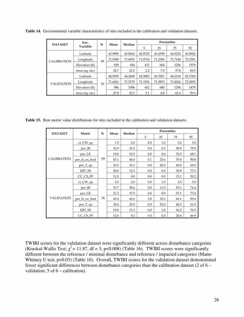
performance of the index. An initial check of dataset comparability determined that the

environmental characteristics were similar between datasets (Mann-Whitney U test; all comparisons,

p>0.05). Similarly, raw values for the selected metrics did not differ between datasets (Mann-

Whitney U test; all comparisons, p>0.05). Mean, median, and percentile comparisons confirmed

Mann-Whitney U test results with only small differences observed in the environmental

characteristics and raw metric values between the calibration and validation datasets (Tables 14 and

15).

26

Table 14. Environmental variable characteristics of sites included in the calibration and validation datasets.

Percentiles

DATASET Env.

Variable N Mean Median

5 25 75 95

Latitude 43.9995 43.8562 42.9723 43.4399 44.5235 45.0924

Longitude 71.5380 71.4933 71.0714 71.2306 71.7144 72.3301

Elevation (ft) 929 924 412 604 1256 1579 CALIBRATION

Area (sq. mi.)

99

24.7 22.5 2.2 7.9 37.8 58.9

Latitude 44.0393 44.2668 42.9082 43.3267 44.6154 45.1760

Longitude 71.6061 71.5179 71.1976 71.3873 71.8426 72.2855

Elevation (ft) 986 1006 462 680 1296 1479 VALIDATION

Area (sq. mi.)

36

27.8 22.5 2.1 6.8 41.4 70.9

Table 15. Raw metric value distributions for sites included in the calibration and validation datasets.

Percentiles

DATASET Metric N Mean Median 5 25 75 95

ct_CW_sp 1.9 2.0 0.0 1.0 3.0 5.0

per_BI 32.9 31.5 0.0 6.5 58.9 79.5

per_GF 19.0 10.3 0.0 0.0 32.9 68.1

per_fs_ex_bnd 47.1 46.0 5.1 25.6 70.0 90.8

per_T_sp 32.0 33.3 0.0 20.0 40.0 60.0

EBT_SS 20.6 12.3 0.0 0.0 30.8 73.1

CALIBRATION

CC_CS_FF

99

11.0 0.0 0.0 0.0 15.1 50.2

ct_CW_sp 2.0 2.0 0.0 1.0 3.0 5.0

per_BI 33.7 38.6 0.0 11.0 53.1 74.4

per_GF 21.3 15.5 0.0 0.0 37.1 73.4

per_fs_ex_bnd 43.4 42.6 2.8 18.3 60.1 89.6

per_T_sp 30.4 25.0 0.0 25.0 40.5 61.0

EBT_SS 19.8 13.3 0.0 1.8 36.2 76.5

VALIDATION

CC_CS_FF

36

12.6 8.2 0.0 0.0 20.6 46.9

TWIBI scores for the validation dataset were significantly different across disturbance categories

(Kruskal-Wallis Test; χ2

= 11.87, df = 3; p<0.008) (Table 16). TWIBI scores were significantly

different between the reference / minimal disturbance and reference / impacted categories (Mann-

Whitney U test, p<0.03) (Table 16). Overall, TWIBI scores for the validation dataset demonstrated

fewer significant differences between disturbance categories than the calibration dataset (2 of 6 –

validation; 5 of 6 – calibration).

27

Table 16. TWIBI score disturbance category comparisons test results for validation dataset.

Comparison Test Test Statistic Significance

Overall Kruskal-Wallis χ2= 11.87 p = 0.008

REF / MIN Mann-Whitney Z = -2.25 p = 0.025

REF / MOD Mann-Whitney Z = -1.64 p = 0.114

REF / IMP Mann-Whitney Z = -3.28 p < 0.001

MIN / MOD Mann-Whitney Z = -0.08 p = 0.968

MIN / IMP Mann-Whitney Z = -1.91 p = 0.066

MOD / IMP Mann-Whitney Z = -1.37 p = 0.181

The 25th

percentile of reference sites was 7.5 index points higher than for the 75th

percentile of

impacted sites (Figure 7). Mean reference and impacted site TWIBI scores were separated by 16.4

index points. None of the impacted sites scored above the 25th

percentile of reference sites and none

of the reference sites scored below the 75th

percentile of impacted sites.

Figure 7. TWIBI scoring summary for sites within each disturbance category (REF = Reference; MIN = minimum;

MOD = moderate; IMP = Impacted) for the validation dataset. . Box and whisker plot - Upper extent of box

is 75th


percentile. Upper whisker = [1.5 x (75th

– 25th

percentile]+ 75th


– 25th


percentile.

Percentiles TYPE N Mean Median

5 25 75 95

REF 11 32.4 32.0 22.0 28.0 38.0 40.0

MIN 9 23.8 24.0 14.0 15.0 31.0 36.0

MOD 10 24.6 27.0 10.0 12.0 32.5 40.0

IMP 6 16.0 15.0 10.0 13.0 20.5 22.0

With the proposed pass-fail threshold of 28, 9 of 11 (82 percent) reference sites exceeded the

criterion, while 3 of 6 (50 percent) of impacted sites failed to achieve the criterion. Contingency

tables indicated that the distribution of reference and test sites exceeding and failing to achieve the

proposed criterion were significantly different (Table 17; χ2; p<0.005).

IMPMODMINREF

40

35

30

25

20

15

10

IBI

sco

re

28

Table 17. Observed and expected frequency of TWIBI threshold attainment (# above; equal to or above proposed

criterion) and non-attainment (# below; below criterion) for reference and impacted sites from the calibration

dataset. Chi-square critical value in parentheses (p=0.0001, df=1)

Site type # above # below Total Chi_square

# observed 9 2 11 Reference

# expected 6 5

# observed 0 6 6 Impacted

# expected 3 3

Total 9 8 17

10.4 (7.879)

5. SUMMARY AND RECOMMENDATIONS

The analysis of fish species relative abundance and frequency of occurrence from 135 wadeable

streams in New Hampshire indicated that the definition of a distinct fish assemblage type, termed

transitional water, is warranted. Transitional water fish assemblages in New Hampshire were

closely allied to the previously identified strict coldwater fish assemblage (NHDES 2007a) in that

they shared several of the most frequently encountered species (e.g. brook trout, slimy sculpin,

blacknose dace). However, transitional water fish assemblages were found to have higher species

richness (mean = 4.6) than strict coldwater fish assemblages (mean = 2.8) and frequently contained

additional species not commonly encountered in strict coldwater environments (e.g. burbot,

longnose dace, longnose sucker). Lyons et al. (2009) reported a similar finding with coolwater

streams having approximately 1.2 times the species richness as coldwater streams in Michigan and

Wisconsin. Yet these streams overlapped in their overall species composition with coldwater

streams. However, unlike the coolwater streams identified by Lyons et al. (2009), which also shared

the characteristics of warmwater streams, transitional water streams in New Hampshire more closely

resembled coldwater streams with warmwater species only occasionally encountered in reference

and minimally disturbed systems.

The observed difference between New Hampshire transitional water fish assemblages and the

coolwater assemblages reported by Lyons et al. (2009) were a result in the approaches to define

these communities. In this report, New Hampshire transitional water assemblages were defined as

streams contained in areas expected to support coldwater fish species throughout the year based on a

predictive model (NHDES 2007b), yet not part of the areas where the strict coldwater index of biotic

integrity (CWIBI) was deemed applicable (NHDES 2007a). In contrast, Lyons et al. (2009) used

species specific laboratory temperature preferences and field studies to define coolwater

assemblages which included both coldwater and warmwater species.

Transitional water fish assemblages are capable of occurring statewide, yet their expected area of

occurrence is focused in the central and northern sections of New Hampshire. The expected area of

occurrence is dependent on a stream’s longitude, latitude, drainage area, and to a lesser extent

elevation. On average, transitional water rivers and streams had a drainage area 4.4 times the size of

29

coldwater streams. Overall, the expected area of occurrence for transitional water fish assemblages

represents approximately 18 percent of New Hampshire’s land area with strict coldwater and

warmwater fish assemblages expected to occur within 48 and 34 percent, respectively. In Michigan

and Wisconsin, Lyons et al. (2009) reported that nearly 65 percent of the stream miles were expected

to support coolwater fish assemblages. Thus, relative to Michigan and Wisconsin and in terms of

the proportion of land area in New Hampshire, transitional water fish assemblages in New

Hampshire are a relatively uncommon natural occurrence.

Streams and rivers where the TWIBI is the most applicable fish condition index will depend on a

site’s latitude, longitude, upstream drainage area, and elevation. However, because distinct

boundaries in biological assemblages rarely exist, there may be instances when best professional

judgement must be used before making a final decision of the most appropriate fish condition index

to be applied in making an ALU determination. In particular, special attention will be paid to sites

where the upstream drainage area is less than 15 square miles. As a general rule for these sites,

when the natural species richness is equal to or less than 4 species, and one or more of these species

includes naturally occurring salmonids or slimy sculpin, the CWIBI may be exchanged for the

TWIBI. Conversely, some streams and rivers where transitional water fish assemblages are

expected to occur, may be more appropriately assessed using a warmwater fish assemblage

condition index. Examples would include flowing waters below natural impoundments, such as a

wetland, or larger streams (>50 square miles) where the natural thermal regimes are too warm to

support coldwater species. The exceptions outlined above will not apply to sites where apparent

shifts in the fish assemblage are potentially linked to anthropogenic impacts.

An eight metric condition index proved useful in discriminating between reference and presumed

impacted sites with overall index scores displaying an inverse relationship to the level of human

disturbance. The selection of eight metrics was within the range of previously developed fish IBIs

(Leonard and Orth 1986; Lyons et al. 1996; Langdon 2001; Daniels et al. 2002; Hughes et al. 2004;

Whittier et al. 2007,), yet lower than the classic biotic index developed by Karr (1981). A

predetermined number of metrics was not targeted prior to index development; rather the number

included in the index was based on performance and redundancy testing for individual metrics.

Overall, metrics associated with thermal preference, tolerance, and trophic class were most

successful at differentiating between reference and impacted sites.

Unlike many previous IBIs (Leonard and Orth 1986; Lyons et al. 1996; Langdon 2001; Daniels et al.

2002), but similar to Whittier et al. (2007) overall species richness did not prove useful in

discriminating between reference and impacted sites. The exclusion of overall richness as a metric

in the TWIBI for New Hampshire was, in part, believed to be a reflection of the naturally low fish

species diversity statewide. In addition, transitional waters, as defined above, represent streams and

rivers with coldwater thermal regimes, and in turn, may serve as a natural restriction in the ability of

warmwater species to thrive in these environments, thus further restricting a finite pool of fish

species.

Similar to the CWIBI, a brook trout age class metric was included in the TWIBI to reflect the level

of reproductive success by an important native, top carnivore, gamefish species. Based on the

results, 48 percent of reference sites and only 20 percent of impacted sites had both adult and YOY

brook trout, respectively. Unlike the other seven metrics included in the index, the brook trout age

class metric is based only on presence or absence, rather than a percentage of species or individuals

within a particular group. The presence of naturally occurring adults and young-of-year (YOY) was

30

considered important in preserving the viability of this important indicator species, while the

presence of just YOY was given an intermediate score, and lack of YOY was given the lowest score.

In recognition that non-native salmonids (brown and rainbow trout) naturally occur, on occasion, in

transitional water fish assemblages, these species should be included in conjunction with brook trout

when computing the TWIBI for all applicable metrics (per_fs_ex_bnd, ct_CW_sp) except the

EBT_SS and brook trout age class metric. For the EBT_SS metric, brown and rainbow trout are to

be excluded without exception. For the brook trout age class metric, brown and rainbow trout may

be included in metric computation when brook trout are absent. The decision to allow the limited

inclusion of non-native salmonids in the TWIBI reflects past fishery management actions which

included the widespread stocking of these species, especially in suspected coldwater streams and

rivers having larger drainage areas. In many cases, for waters where temperatures remained cold

enough annually, these species established naturally reproducing populations and have proliferated.

As a result, their presence represents a positive indicator of biological condition and should be

reflected in the overall index score. However, the inclusion of recently stocked individuals is not

permitted for any salmonid species. This includes brook trout and Atlantic salmon. These actions

reflect recent fishery management decisions and not a natural ecological consequence of

environmental conditions (Halliwell et al. 1999).

The index, as constructed, represents one that minimizes inter-metric redundancy and maximizes

efficiency. None of the metrics included in the TWIBI had a correlation coefficient in excess of

0.75. The lack of metric redundancy indicates that each component of the index represents a unique

expression of the ecological characteristics of the fish assemblage. Further, the individual metrics

selected for inclusion into the index proved to be responsive to increases in environmental stressors

based on the narrative impact rating categories. Of the eight metrics included in the index, each was

able to clearly separate reference and impacted sites and was among the strongest indicators in doing

so based on an objective testing process. While this process differs from that employed by Whittier

et al. (2007), both attempt to achieve the same result; namely the selection of metrics, across broad

ecological categories, that combine to represent the important qualities of an minimally impacted

biological community and capable of detecting a departure from this condition.

Overall the TWIBI developed for New Hampshire streams bears some resemblance to the mixed

waters index used by the Vermont Department of Environmental Conservation (VTDEC 2007) in

terms of the total number of metrics (NH – eight, VT – nine), individual metrics, and index threshold

(NH – 28, VT – 30). The similarity of these two indices is partially a reflection of fish assemblage

similarity. With the exception of the Champlain drainage in Vermont, New Hampshire and Vermont

share many of the same fish species. In both states, water temperature, ultimately, represents the

primary natural environmental factor that structures fish assemblages. Elevation and watershed size,

while important in structuring fish assemblages, are more appropriately considered proximal

variables that influence water temperature. Thus, where the thermal regimes are similar, the

resulting native fish assemblages in Vermont and New Hampshire streams are likely to be composed

of many of the same species or of species filling similar ecological niches. In turn, while separate

indices have been developed by their respective state agencies, they are likely transferable across

state lines, and, more importantly, the results can be compared. Furthermore, it does not seem

implausible that either of these indices could be applied throughout the New England states with

minor adjustments where similar thermal regimes can be identified. Daniels et al. (2002)

recommended similar a similar application of his Mid-Atlantic Slope IBI with modification in order

to account for the natural ecosystem features and study objectives.

31

The recommended index threshold of 28 was based on the twenty-fifth percentile of all reference

sites and corresponds to previously developed biological indices for fish and macroinvertebrates in

New Hampshire. Hughes et al. 2004 provided examples of how manipulating threshold criteria can

lead to varying amounts of stream miles considered to be impaired. Without a doubt the selection of

any statistical threshold (i.e., x-percentile, # standard deviations) is a subjective decision that implies

a level of confidence in the index’s performance, natural variability, sampling efficiency, and an

acceptable reduction in biological condition. For the TWIBI, and other biological indices developed

by the NHDES, it is believed that a twenty-fifth percentile threshold is acceptable for the

determination of aquatic life use. A lower or higher threshold would likely be under- or

overprotective of the resource, respectively. Thus, the selection of this threshold is an attempt to

balance an acceptable biological condition while concurrently taking into account largely

uncontrollable sources of index variability such as sampling effectiveness, unmeasured components

of ecosystem health (i.e. trophic dynamics), and regional environmental impacts.

Mean index scores from the calibration dataset were 32 for reference sites and 18 for impacted sites.

Based on these results, and in conjunction with those observed from the validation dataset, it can be

concluded that the index was capable of clearly distinguishing changes in fish assemblage structure

and function as the level of disturbance increased. The selection of the 25th percentile of reference

site index scores as a criterion translated into 9 of 10 impacted sites from the calibration dataset

failing to achieve the threshold of 28. Overall, the threshold chosen for the TWIBI was determined

to be appropriate in defining an acceptable versus unacceptable level of departure from the “natural”

condition. However, as with any biological index, an “attainment” threshold is a human-imposed

decision criterion along a gradient of ecological structure and function. As a result, a single numeric

representation of overall assemblage condition should be considered in concert with the actual raw

data when making final impairment or regulatory decisions.

The TWIBI establishes a proposed set of guidelines to define a unique fish assemblage, a suite of

metrics to measure biological condition, and a criterion to determine the level of departure from

minimally impacted sites. These guidelines, measures, and associated thresholds are, however,

based on current environmental conditions. In evaluating the data, geographically widespread

unnatural perturbations to these conditions include regional and global impacts such as acid

deposition and climate change, respectively. The effects of these impacts are difficult, if not

impossible, to account for, and therefore, should be considered as unknown elements that may have

contributed to the geographic boundaries of the transitional water fish assemblage defined herein, as

well as metric selection and threshold determination. Further, as these impacts are likely to

continue, and perhaps worsen, modifications to the index will be necessary to account for changes in

natural fish distributions, assemblage structure and function, and expectations in biological

condition.

The TWIBI will serve as a partial numeric interpretation of the NHDES’s current narrative water

quality criteria relating to the biological integrity (Env - Wq 1703.19) of aquatic communities for 1st

through 4th

order wadeable streams meeting the definition of a transitional water fish assemblage.

The index is designed to accurately and precisely describe the biological condition of this

assemblage type through eight unique ecological measures (metrics). Other indices, such as the

NHDES’ benthic IBI, or physical and chemical water quality measures may be coupled with the

TWIBI for the determination of aquatic life use and used in completing federally-required water

quality reports, state-level regulatory actions, permit limits, and general water quality planning

activities.

32

6. REFERENCES

Bain, M. B. 1996. Fish codes and classes: File documentation, sources, and notes. New York

Cooperative Fish and Wildlife Research Unit, Cornell University, Ithaca, NY.

Balon, E. K. 1975. Reproductive guilds of fishes: a proposal and definition. Journal of the Fisheries

Research Board of Canada 32:821-864.

Barbour, M. T, J. B. Stribling, and J. R. Karr. 1995. Multimetric approach for establishing

biocriteria and measuring biological condition. Pages 63-77 in W. S. Davis and T. P. Simon, editor.

Biological assessment and criteria: Tools for water resource planning and decision making. CRC

Press, Boca Raton, Florida.

Barbour, M. T., J. Gerristen, B. D. Snyder, and J. B. Stribling. 1999. Rapid bioassessment protocols

for use in streams and wadeable rivers: periphyton, benthic macroinvertebrates and fish, second

edition. EPA 841-B-99-002. U. S. Environmental Protection Agency; Office of Water;

Washington, D.C.

Daniels, R. A., K. Riva-Murrary, D.B. Halliwell, D.L. Vana-Miller, M.D. Bilger. 2002. An index

of biological integrity for northern mid-Atlantic slope drainages. Transactions of the American

Fisheries Society131:1044-1060.

Halliwell, D. B., R. W. Langdon, R. A. Daniels, J. P. Kurtenbach, and R. A. Jacobson. 1999.

Classification of freshwater fish species of the Northeastern United States for use in the development

of indices of biological integrity, with regional applications. Pages 301-333 in T. P. Simon, editor.

Assessing the sustainability and biological integrity of water resources using fish communities.

CRC Press, Boca Raton, Florida.

Hughes, R. M., S. Howlin, and P. R. Kaufmann. 2004. A biointegrity index (IBI) for coldwater

streams of western Oregon and Washington. Transactions of the American Fisheries Society

133:1497-1515.

Karr, J. R. 1981. Assessment of biotic integrity using fish communities. Fisheries 6:28-30.

Mundahl, N. D. and T. P. Simon. 1999. Development and application of an index of biotic integrity

for coldwater streams of the upper Midwestern United States. Pages 383-411 in T. P. Simon, editor.

Assessing the sustainability and biological integrity of water resources using fish communities.

CRC Press, Boca Raton, Florida.

NHDES. 2007a. Coldwater fish assemblage index of biotic integrity for New Hampshire wadeable

streams. New Hampshire Department of Environmental Services, Concord, NH. Publication #R-

WD-07-33.

NHDES. 2007b. Predicted coldwater fish indicator species presence in New Hampshire wadeable

streams. New Hampshire Department of Environmental Services, Concord, NH. Publication #R-

WD-07-38.

33

Langdon, R. W. 2001. A preliminary index of biological integrity for fish assemblages of small

coldwater streams in Vermont. Northeastern Naturalist 8:219:232.

Leonard, P. M. and D. J. Orth. 1986. Application and testing of an index of biotic integrity in small,

coolwater streams. Transactions of the American Fisheries Society 115:401-414.

Lyons, J., L. Wang, and T. D. Simonson. 1996. Development and validation of an index of biotic

integrity for coldwater streams in Wisconsin. North American Journal of Fisheries Management

16:241-256.

Lyons, J., T. Zorn, J. Stewart, P. Seelbach, K. Wehrly, and L. Wang. 2009. Defining and

characterizing coolwater streams and their fish assemblages in Michigan and Wisconsin, USA.

North American Journal of Fisheries Management 29:1130-1151.

Simon, T. P. 1999. Assessment of Balon’s reproductive guilds with application to Midwestern

North American freshwater fishes. Pages 97-121 in T. P. Simon, editor. Assessing the sustainability

and biological integrity of water resources using fish communities. CRC Press, Boca Raton, Florida.

Stoddard, J. L., D. P. Larsen, C. P. Hawkins, R. K. Johnson, and R. H. Norris. 2006. Setting

expectations for the ecological condition of streams: The concept of reference condition. Ecological

Applications 16:1267-1276.

VT DEC. 2004. Biocriteria for fish and macroinvertebrate assemblages in Vermont wadeable

streams and rivers – Development phase. Agency report. Water Quality Division, Biomonitoring

and Aquatic Studies Section, Waterbury, Vermont.

Whittier, T. R., R. M. Hughes, J. L. Stoddard, G. A. Lomnicky, D. V. Peck, and A. T. Herlihy.

2007. A structured approach for developing indices of biotic integrity: Three examples from

streams and rivers in the western USA. Transactions of the American Fisheries Society 136:718-

735.

34

Appendix A. Candidate metrics and their respective abbreviation, expected response organized by major category.

Metric Abbreviation Expected response Metric group Variable type

Percent introduced generalist feeder individuals per_intro_GF - aliens continuous

Percent introduced top carnivore individuals per_intro_TC - aliens continuous

Percent introduced warmwater individuals per_intro_WW - aliens continuous

Perccent introduced macrohabitat generalists per_intro_mg - aliens continuous

Number of Cyprinid species num_cyp_sp - Composition discrete

Percentage of Cyprinid species per_cyp_sp - Composition continuous

Percentage of the dominant species per_dom_sp - Composition continuous

Percentage of Blacknose dace BND - Composition continuous

Percentage of Burbot BRB + Composition continuous

Percentage of Brown trout BT + Composition continuous

Percentage of Creek chub CC - Composition continuous

Percentage of Common shiners CS - Composition continuous

Percentage of White suckers CWS - Composition continuous

Percentage of Brook trout EBT + Composition continuous

Percentage of Fallfish FF - Composition continuous

Percentage of Longnose dace LND + Composition continuous

Percentage of Longnose suckers LNS + Composition continuous

Percentage of Rainbow trout RT + Composition continuous

Percentage of Slimy sculpin SS + Composition continuous

Percentage of Brook trout and Slimy sculpin EBT_SS + Composition continuous

Percentage of Creek chub, Common shiner, Fallfish CC_CS_FF - Composition continuous

Percentage of Creek chub, Common shiner, Fallfish, Blacknose dace CC_CS_FF_BND - Composition continuous

Percentage of speleophil spawners (hole nesters) (Balon 1975 - B.2.7) per_hol_dig reproduction continuous

Percentage of non-obligate substrate spawners (Balon 1975 - A.1.4) per_nob_sub reproduction continuous

Percentage of polyphil spawners (nest builders on misc. materail (Balon 1975 - B.2.2) per_nst_sub reproduction continuous

Percentage of phytophil spawners (obligatory plant spawners) (Balon 1975 - A.1.5) per_ob_plt reproduction continuous

Percentage of simple lithophilic spawner individuals (non-guarding rock/gravel spawners) (Balon 1975 - A.1.2 & A.1.3) per_simp_litho + reproduction continuous

Percentage of specialized lithophilic spawner individuals (guarding rock/gravel spawners) (Balon 1975 - B.1.3) per_spec_litho + reproduction continuous

Number of fluvial specialist species (Based on Bain 1996) num_fs_sp + richness discrete

Number of fluvial dependant species (Based on Bain 1996) num_fd_sp + richness discrete

Number of fluvial specialist + dependant species (Based on Bain 1996) num_fs_fd_sp + richness discrete

Total number of species num_sp_all + richness discrete

Total number of native (non-introduced) species num_sp_nat + richness discrete

Number of macrohabitat generalist species (Based on Bain 1996) num_mg_sp - richness discrete

Percentage of fluvial dependant + specialist species (Based on Bain 1996) per_fd_fs_sp + streamflow continuous

Percentage of macrohabitat generalist species (Based on Bain 1996) per_mg_sp - streamflow continuous

Percentage of fluvial specialist individuals less blacknose dace per_fs_ex_bnd + streamflow continuous

Percentage of rheophilic individuals (Based on Whittier et al. 2007) per_r + streamflow continuous

Percentage of flowing water preferring individuals (Based on Whittier et al. 2007) per_x + streamflow continuous

35

Appendix A (con’t).

Metric Abbreviation Expected response Metric group Variable type

Percentage of rheophilic + flowing water preferring individuals (Based on Whittier et al. 2007) per_r_x + streamflow Continuous

Percentage of non-lotic individuals per_no_lotic - streamflow continuous

Percentage of fluvial dependant individuals (Based on Bain 1996) per_fd + streamflow continuous

Percentage of fluvial specialist individuals (Based on Bain 1996) per_fs + streamflow continuous

Percentage of macrohabitat generalist individuals (Based on Bain 1996) per_mg - streamflow continuous

Percentage of fluvial dependant + specialist individuals (Based on Bain 1996) per_fd_fs + streamflow continuous

Percentage of coldwater species per_cw_sp + thermal continuous

Percentage of eurythermal species per_et_sp - thermal continuous

Percentage of warmwater species per_ww_sp - thermal continuous

Percentage of coldwater individuals per_CW + thermal continuous

Number of coldwater species num_CW + thermal discrete

Percentage of warmwater individuals per_WW - thermal continuous

Number of warmwater species num_WW - thermal discrete

Percentage of eurythermal individuals per_ET - thermal continuous

Number of eurythermal species num_ET - thermal discrete

Percentage of intolerant species per_I_sp + tolerance continuous

Percentage of moderately tolerant species per_M_sp - tolerance continuous

Percentage of tolerent species per_T_sp - tolerance continuous

Percentage of intolerant individuals per_I + tolerance continuous

Number of intolerant species num_I + tolerance discrete

Percentage of moderately tolerant individuals per_M - tolerance continuous

Number of moderately tolerant species num_M - tolerance discrete

Percentage of tolerant individuals per_T - tolerance continuous

Number of tolerant species num_T - tolerance discrete

Percentage of tolerant generalist feeder individuals per_tol_GF - trophic continuous

Percentage of benthic insectivore individuals per_BI + trophic continuous

Percentage of generalist feeder individuals per_GF - trophic continuous

Percentage of obligate insectivore individuals per_OI + trophic continuous

Pecentage of top carnivore individuals per_TC + trophic continuous

Number of benthic insectivore species ct_BI_sp + trophic discrete

Number of generalist feeder species ct_GF_sp - trophic discrete

Number of obligate insectivore species ct_OI_sp + trophic discrete

Number of top carnivore species ct_TC_sp + trophic discrete

36

Appendix B. Autecological fish characteristics.

Origin Thermal Preference Tolerance Reproductive strategy1

Abbreviation Type Abbreviation Type Abbreviation Type Abbreviation Type

N Native CW Coldwater I Intolerant S_L

Simple

Lithophil

(coarse

substrate

spawners,

non-

guarders)

ET Eurythermal M Moderately

Tolerant I Introduced

WW Warmwater T Tolerant

H_D Hole

nester

Trophic Class Streamflow Preference2 Streamflow Preference

3

Abbreviation Type Abbreviation Type Abbreviation Type

BI Benthic

insectivore L Prefers large rivers fd Fluvial dependant

GF Generalist feeder R Rheophilic – prefers fast

flowing waters fs Fluvial specialist

OI Obligate

insectivore

TC Top carnivore

X Prefers flowing waters mg Macrohabitat

generalist

1- Simon 1999; based on Balon 1975 2- Whittier et al. 2007 3- Bain 1996

37

Appendix C. Details of objective metric testing combinations for partial determination of metrics selected for

inclusion into the TWIBI.

For positive (+) response metrics:

Combination Compare Mathematical Expression Response

Evaluation

Expected

Response

1 Means Mean (Reference sites) –

Mean (Impacted sites)

2 Medians Median (Reference sites) –

Median (Impacted sites)

3 25

th vs. 75

th

percentiles

25th

percentile (Reference sites) –

75th

percentile (Impacted Sites

4 Mean vs.

75th

percentile

Mean (Reference sites) –

75th

percentile (Impacted sites)

5 Median vs.

75th

percentile

Median (Reference sites) –

75th

percentile (Impacted sites)

Sign (+ / -) and

magnitude +

For negative (-) response metrics:

Combination Compare Mathematical Expression Response

Evaluation

Expected

Response

1 Means Mean (Impacted sites) –

Mean (Reference sites)

2 Medians Median (Impacted sites) –

Median (Reference sites)

3 25

th vs. 75

th

percentiles

25th

percentile (Impacted sites) –

75th

percentile (Reference Sites

4 Mean vs.

75th

percentile

Mean (Impacted sites) –

75th

percentile (Reference sites)

5 Median vs.

75th

percentile

Median (Impacted sites) –

75th

percentile (Reference sites)

Sign (+ / -) and

magnitude +

38

Appendix D. Spearman’s correlation coefficients for 20 candidate metrics. Bolded text indicates metrics included in the TWIBI. Grey shaded cells indicate

correlation coefficients >0.75.

METRIC↓→ EBT_SS CC_CS_FF per_r per_fs_ex_bnd per_cw_sp ct_CW_sp per_CW per_I per_tol_GF per_T_sp per_GF per_BI

Correlation Coefficient -0.01 0.06 0.16 0.45 0.35 0.72 0.93 0.04 -0.37 0.05 -0.14 EBT_SS

Sig. (2-tailed) 0.938 0.752 0.391 0.011 0.054 0.000 0.000 0.851 0.041 0.800 0.467

Correlation Coefficient -0.01 -0.38 -0.25 -0.40 -0.06 -0.25 -0.08 0.62 0.32 0.51 -0.48 CC_CS_FF

Sig. (2-tailed) 0.938 0.035 0.166 0.027 0.752 0.167 0.677 0.000 0.080 0.003 0.006

Correlation Coefficient 0.06 -0.38 0.63 -0.08 -0.39 -0.25 0.10 -0.43 -0.08 -0.68 0.23 per_r

Sig. (2-tailed) 0.752 0.035 0.000 0.660 0.031 0.183 0.593 0.015 0.688 0.000 0.208

Correlation Coefficient 0.16 -0.25 0.63 0.06 0.07 0.00 0.31 -0.28 -0.40 -0.41 0.61 per_fs_ex_bnd

Sig. (2-tailed) 0.391 0.166 0.000 0.734 0.722 0.994 0.092 0.132 0.028 0.024 0.000

Correlation Coefficient 0.45 -0.40 -0.08 0.06 0.68 0.75 0.55 -0.38 -0.72 -0.13 0.01 per_cw_sp

Sig. (2-tailed) 0.011 0.027 0.660 0.734 0.000 0.000 0.001 0.034 0.000 0.477 0.948

Correlation Coefficient 0.35 -0.06 -0.39 0.07 0.68 0.57 0.50 0.04 -0.53 0.25 -0.04 ct_CW_sp

Sig. (2-tailed) 0.054 0.752 0.031 0.722 0.000 0.001 0.004 0.832 0.002 0.180 0.835

Correlation Coefficient 0.72 -0.25 -0.25 0.00 0.75 0.57 0.78 -0.08 -0.53 0.10 -0.10 per_CW

Sig. (2-tailed) 0.000 0.167 0.183 0.994 0.000 0.001 0.000 0.669 0.002 0.610 0.599

Correlation Coefficient 0.93 -0.08 0.10 0.31 0.55 0.50 0.78 -0.02 -0.49 -0.01 -0.12 per_I

Sig. (2-tailed) 0.000 0.677 0.593 0.092 0.001 0.004 0.000 0.915 0.005 0.944 0.504

Correlation Coefficient 0.04 0.62 -0.43 -0.28 -0.38 0.04 -0.08 -0.02 0.60 0.57 -0.21 per_tol_GF

Sig. (2-tailed) 0.851 0.000 0.015 0.132 0.034 0.832 0.669 0.915 0.000 0.001 0.258

Correlation Coefficient -0.37 0.32 -0.08 -0.40 -0.72 -0.53 -0.53 -0.49 0.60 0.06 -0.14 per_T_sp

Sig. (2-tailed) 0.041 0.080 0.688 0.028 0.000 0.002 0.002 0.005 0.000 0.753 0.452

Correlation Coefficient 0.05 0.51 -0.68 -0.41 -0.13 0.25 0.10 -0.01 0.57 0.06 -0.29

Sig. (2-tailed) 0.800 0.003 0.000 0.024 0.477 0.180 0.610 0.944 0.001 0.753 0.108 per_GF

N 31 31 31 31 31 31 31 31 31 31 31

Correlation Coefficient -0.14 -0.48 0.23 0.61 0.01 -0.04 -0.10 -0.12 -0.21 -0.14 -0.29 per_BI

Sig. (2-tailed) 0.467 0.006 0.208 0.000 0.948 0.835 0.599 0.504 0.258 0.452 0.108

39

Appendix E. TWIBI sites, associated characteristics, and index scores.

Master ID Project Agency ID Stream Name Town

Disturbance Category Site_type

repeat (n=no; r= repeat

Elevation (ft)

Drainage area (sq. mi.)

Longitude (dd.dddd)

Latitude (dd.dddd)

Probability supports coldwater fish species

TWIBI score

s101 DES 00C-50 CLARK BROOK HAVERHILL IMP VALIDATION n 483 17.1 72.0245 44.0895 0.995 14

s102 DES 98P-79 CHURCHILL BROOK BROOKFIELD REF CALIBRATION n 578 4.9 71.0714 43.5472 0.670 20

s103 DES 00M-18 TANNERY BROOK BOSCAWEN IMP CALIBRATION n 283 8.0 71.6290 43.3234 0.727 18

s104 DES 98P-79 CHURCHILL BROOK BROOKFIELD REF VALIDATION r 578 4.9 71.0714 43.5472 0.670 28

s105 DES 00M-38 WILLEY BROOK WOLFBORO MIN CALIBRATION n 611 6.6 71.1598 43.6234 0.770 14

s107 DES 00M-8 SANBORN BROOK LOUDON MOD CALIBRATION n 604 5.3 71.3873 43.3267 0.624 10

s109 DES 01M-01 OWL BROOK HOLDERNESS MIN CALIBRATION n 631 7.2 71.6292 43.7322 0.960 32

s114 DES 98S-65 BEECH RIVER OSSIPEE MIN CALIBRATION n 520 15.0 71.1565 43.7271 0.722 20

s115 DES 01M-07 MOOSILAUKE RIVER WOODSTOCK MIN CALIBRATION n 815 17.1 71.7119 44.0292 0.983 32

s116 DES 99C-23 PARTRIDGE BROOK WESTMORELAND MOD CALIBRATION n 459 16.5 72.4311 42.9497 0.677 12

s117 DES 01M-17 COCKERMOUTH RIVER GROTON MIN VALIDATION n 670 13.3 71.8499 43.7074 0.959 36

s118 DES 99M-18 BEAVER BROOK ALTON MOD CALIBRATION n 580 7.5 71.2006 43.5344 0.688 20

s119 DES 01S-13 SACO RIVER-EAST BRANCH BARTLETT REF CALIBRATION n 520 39.6 71.1591 44.0979 0.642 32

s120 DES 99M-28 DUDLEY BROOK DEERING MOD CALIBRATION n 831 8.7 71.8083 43.0997 0.577 24

s121 DES 03M-TREND03 SANBORN BROOK LOUDON MOD CALIBRATION r 604 5.3 71.3873 43.3267 0.624 14

s122 DES 99M-46 SMITH BROOK GRAFTON MOD CALIBRATION n 839 9.4 71.9525 43.5581 0.955 20

s123 DES 03M-TREND03 SANBORN BROOK LOUDON MOD VALIDATION r 604 5.3 71.3873 43.3267 0.624 20

s124 DES 99M-47 TIOGA RIVER BELMONT MOD CALIBRATION n 783 4.1 71.4282 43.4806 0.823 10

s125 DES 03M-TREND03 SANBORN BROOK LOUDON MOD VALIDATION r 604 5.3 71.3873 43.3267 0.624 12

s126 DES 99M-48 NIGHTHAWK HOLLOW GILMANTON MOD VALIDATION n 709 3.9 71.3532 43.4292 0.742 12

s127 DES 04c-01 BLOW ME DOWN BROOK CORNISH MOD CALIBRATION n 423 25.0 72.3765 43.5159 0.937 18

s128 DES 99M-5 STIRRUP IRON BRO BOSCAWEN MIN CALIBRATION n 417 5.9 71.6610 43.3759 0.825 22

s129 DES 04c-11 AMMONOOSUC RIVER CARROLL MOD VALIDATION n 1549 37.0 71.4712 44.2690 0.935 32

s130 DES 99M-51 AMEY BROOK HENNIKER IMP CALIBRATION n 427 12.0 71.8211 43.1919 0.627 14

s131 DES 05A-13 SWIFT DIAMOND RIVER SECOND COLLEGE GRANT REF CALIBRATION n 1360 26.3 71.0853 44.9426 0.997 28

s133 DES 05A-15 DEAD DIAMOND RIVER SECOND COLLLEGE GRANT REF CALIBRATION n 1512 40.4 71.1610 44.8664 0.989 24

40




Elevation (ft)


Longitude (dd.dddd)

Latitude (dd.dddd)


TWIBI score

s134 DES 99M-8 BRADLEY BROOK ANDOVER MIN CALIBRATION n 853 2.2 71.8247 43.4067 0.928 28

s136 DES 99M-8 BRADLEY BROOK ANDOVER MIN CALIBRATION r 853 2.2 71.8247 43.4067 0.928 26

s137 DES 05C-11 OTTER BROOK LANCASTER IMP CALIBRATION n 924 24.9 71.5412 44.4812 0.994 20

s139 DES 06c-13 LITTLE SUGAR RIVER CHARLESTOWN MOD VALIDATION n 343 29.3 72.3853 43.3057 0.775 34

s141 DES 06c-17 MINK BROOK HANOVER IMP VALIDATION n 538 15.5 72.2679 43.6908 0.985 20

s146 DES NH HEX 28.03 AMES BROOK ASHLAND MOD CALIBRATION n 515 5.6 71.6308 43.6920 0.957 24

s147 DES 07m-03 PUNCH BROOK FRANKLIN MIN CALIBRATION n 412 8.5 71.6690 43.4128 0.820 26

s149 DES 07m-07 COLLINS BROOK FRANCESTOWN MIN VALIDATION n 811 7.2 71.8308 43.0124 0.518 16

s151 DES 07m-09 HAYWARD BROOK CONCORD MOD CALIBRATION n 329 12.1 71.5575 43.2885 0.549 16

s152 DES NH HEX 35.01 CHURCHILL BROOK BROOKFIELD MOD CALIBRATION n 533 7.0 71.0613 43.5499 0.621 30

s153 DES 07m-11 SALMON BROOK SANBORNTON IMP CALIBRATION n 589 18.2 71.6218 43.5159 0.731 16

s155 DES 07m-13 S BR BAKER RIVER WENTWORTH MIN CALIBRATION n 793 31.3 71.9320 43.8185 0.909 26

s157 DES 07s-05 COLD RIVER CENTER SANDWICH MOD CALIBRATION n 668 29.8 71.3645 43.8562 0.707 24

s163 DES 98C-1 INDIAN STREAM PITTSBURG REF CALIBRATION n 1307 63.5 71.4097 45.0924 0.986 36

s165 DES 98C-1 INDIAN STREAM PITTSBURG REF VALIDATION r 1307 63.5 71.4097 45.0924 0.986 28

s167 DES 98C-10 SIMMS STREAM COLUMBIA MIN CALIBRATION n 1266 28.0 71.4933 44.8494 0.999 38

s169 DES 98C-10 SIMMS STREAM COLUMBIA MIN CALIBRATION r 1266 28.0 71.4933 44.8494 0.999 40

s173 DES 98C-14 STRATFORD BOG BROOK STRATFORD REF CALIBRATION r 1011 16.9 71.5379 44.6783 0.999 40

s175 DES 98C-15 NASH STREAM STRATFORD MIN CALIBRATION n 1377 38.4 71.4539 44.6758 0.990 40

s179 DES 98C-18 UPPER AMMONOOSUC RIVER BERLIN REF CALIBRATION n 1157 48.7 71.2879 44.5235 0.912 34

s181 DES 98C-18 UPPER AMMONOOSUC RIVER BERLIN REF CALIBRATION r 1157 48.7 71.2879 44.5235 0.912 34

s183 DES 98C-19 AMMONOOSUC RIVER CARROLL MOD VALIDATION n 1466 43.5 71.4927 44.2647 0.892 32

s185 DES 98C-2 INDIAN STREAM PITTSBURG REF VALIDATION n 1229 67.4 71.4354 45.0744 0.980 26

s187 DES 98C-2 INDIAN STREAM PITTSBURG REF VALIDATION r 1229 67.4 71.4354 45.0744 0.980 32

s191 DES 98C-36 ISREAL RIVER JEFFERSON MIN VALIDATION n 1057 70.5 71.4989 44.4125 0.593 28

s193 DES 98C-36 ISREAL RIVER JEFFERSON MIN CALIBRATION r 1057 70.5 71.4989 44.4125 0.593 22

s195 DES 98C-4 PERRY STREAM PITTSBURG REF CALIBRATION n 1579 24.4 71.3200 45.1043 1.000 36

s197 DES 98C-6 CONNECTICUT RIVER PITTSBURG MIN CALIBRATION n 1644 59.9 71.2071 45.1190 0.984 36

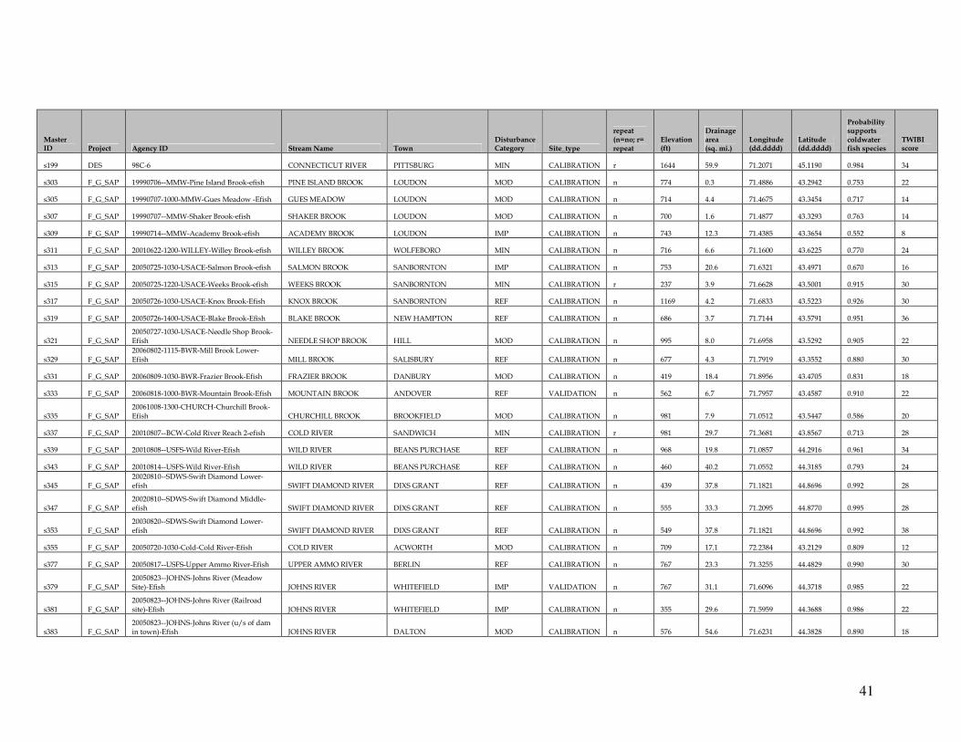
41




Elevation (ft)


Longitude (dd.dddd)

Latitude (dd.dddd)


TWIBI score

s199 DES 98C-6 CONNECTICUT RIVER PITTSBURG MIN CALIBRATION r 1644 59.9 71.2071 45.1190 0.984 34

s303 F_G_SAP 19990706--MMW-Pine Island Brook-efish PINE ISLAND BROOK LOUDON MOD CALIBRATION n 774 0.3 71.4886 43.2942 0.753 22

s305 F_G_SAP 19990707-1000-MMW-Gues Meadow -Efish GUES MEADOW LOUDON MOD CALIBRATION n 714 4.4 71.4675 43.3454 0.717 14

s307 F_G_SAP 19990707--MMW-Shaker Brook-efish SHAKER BROOK LOUDON MOD CALIBRATION n 700 1.6 71.4877 43.3293 0.763 14

s309 F_G_SAP 19990714--MMW-Academy Brook-efish ACADEMY BROOK LOUDON IMP CALIBRATION n 743 12.3 71.4385 43.3654 0.552 8

s311 F_G_SAP 20010622-1200-WILLEY-Willey Brook-efish WILLEY BROOK WOLFEBORO MIN CALIBRATION n 716 6.6 71.1600 43.6225 0.770 24

s313 F_G_SAP 20050725-1030-USACE-Salmon Brook-efish SALMON BROOK SANBORNTON IMP CALIBRATION n 753 20.6 71.6321 43.4971 0.670 16

s315 F_G_SAP 20050725-1220-USACE-Weeks Brook-efish WEEKS BROOK SANBORNTON MIN CALIBRATION r 237 3.9 71.6628 43.5001 0.915 30

s317 F_G_SAP 20050726-1030-USACE-Knox Brook-Efish KNOX BROOK SANBORNTON REF CALIBRATION n 1169 4.2 71.6833 43.5223 0.926 30

s319 F_G_SAP 20050726-1400-USACE-Blake Brook-Efish BLAKE BROOK NEW HAMPTON REF CALIBRATION n 686 3.7 71.7144 43.5791 0.951 36

s321 F_G_SAP 20050727-1030-USACE-Needle Shop Brook-Efish NEEDLE SHOP BROOK HILL MOD CALIBRATION n 995 8.0 71.6958 43.5292 0.905 22

s329 F_G_SAP 20060802-1115-BWR-Mill Brook Lower-Efish MILL BROOK SALISBURY REF CALIBRATION n 677 4.3 71.7919 43.3552 0.880 30

s331 F_G_SAP 20060809-1030-BWR-Frazier Brook-Efish FRAZIER BROOK DANBURY MOD CALIBRATION n 419 18.4 71.8956 43.4705 0.831 18

s333 F_G_SAP 20060818-1000-BWR-Mountain Brook-Efish MOUNTAIN BROOK ANDOVER REF VALIDATION n 562 6.7 71.7957 43.4587 0.910 22

s335 F_G_SAP 20061008-1300-CHURCH-Churchill Brook-Efish CHURCHILL BROOK BROOKFIELD MOD CALIBRATION n 981 7.9 71.0512 43.5447 0.586 20

s337 F_G_SAP 20010807--BCW-Cold River Reach 2-efish COLD RIVER SANDWICH MIN CALIBRATION r 981 29.7 71.3681 43.8567 0.713 28

s339 F_G_SAP 20010808--USFS-Wild River-Efish WILD RIVER BEANS PURCHASE REF CALIBRATION n 968 19.8 71.0857 44.2916 0.961 34

s343 F_G_SAP 20010814--USFS-Wild River-Efish WILD RIVER BEANS PURCHASE REF CALIBRATION n 460 40.2 71.0552 44.3185 0.793 24

s345 F_G_SAP 20020810--SDWS-Swift Diamond Lower-efish SWIFT DIAMOND RIVER DIXS GRANT REF CALIBRATION n 439 37.8 71.1821 44.8696 0.992 28

s347 F_G_SAP 20020810--SDWS-Swift Diamond Middle-efish SWIFT DIAMOND RIVER DIXS GRANT REF CALIBRATION n 555 33.3 71.2095 44.8770 0.995 28

s353 F_G_SAP 20030820--SDWS-Swift Diamond Lower-efish SWIFT DIAMOND RIVER DIXS GRANT REF CALIBRATION n 549 37.8 71.1821 44.8696 0.992 38

s355 F_G_SAP 20050720-1030-Cold-Cold River-Efish COLD RIVER ACWORTH MOD CALIBRATION n 709 17.1 72.2384 43.2129 0.809 12

s377 F_G_SAP 20050817--USFS-Upper Ammo River-Efish UPPER AMMO RIVER BERLIN REF CALIBRATION n 767 23.3 71.3255 44.4829 0.990 30

s379 F_G_SAP 20050823--JOHNS-Johns River (Meadow Site)-Efish JOHNS RIVER WHITEFIELD IMP VALIDATION n 767 31.1 71.6096 44.3718 0.985 22

s381 F_G_SAP 20050823--JOHNS-Johns River (Railroad site)-Efish JOHNS RIVER WHITEFIELD IMP CALIBRATION n 355 29.6 71.5959 44.3688 0.986 22

s383 F_G_SAP 20050823--JOHNS-Johns River (u/s of dam in town)-Efish JOHNS RIVER DALTON MOD CALIBRATION n 576 54.6 71.6231 44.3828 0.890 18

42




Elevation (ft)


Longitude (dd.dddd)

Latitude (dd.dddd)


TWIBI score

s385 F_G_SAP 20050908--JOHNS-Johns River (Brown Street)-Efish JOHNS RIVER WHITEFIELD IMP CALIBRATION n 986 50.1 71.6224 44.3772 0.923 24

s387 F_G_SAP 20050908--JOHNS-Johns River (Sand Pit Site)-Efish JOHNS RIVER DALTON MIN CALIBRATION n 779 58.1 71.6277 44.3936 0.862 20

s389 F_G_SAP 20050929-1100-BCW-Swift River-efish SWIFT RIVER TAMWORTH REF VALIDATION n 620 26.5 71.2905 43.8862 0.753 40

s391 F_G_SAP 20060810-1240-JV-S. Branch Baker River-Efish BAKER RIVER WENTWORTH MIN CALIBRATION n 589 38.6 71.9156 43.8241 0.832 18

s395 F_G_SAP 20060810-1400-JV-S. Branch Baker River-Efish BAKER RIVER DORCHESTER MIN CALIBRATION n 651 18.5 71.9245 43.8001 0.967 16

s425 F_G_SAP 20060922-1020-BCW-Swift River-Efish SWIFT RIVER TAMWORTH REF CALIBRATION n 1236 25.2 71.2972 43.8927 0.785 40

s427 F_G_SAP 20070817-1100-REG1-Swift Diamond River Lower-Efish

SWIFT DIAMOND RIVER LOWER DIXS GRANT REF CALIBRATION n 1000 37.8 71.1815 44.8695 0.992 30

s429 F_G_SAP 20070817-845-REG1-Swift Diamond River Upper-Efish

SWIFT DIAMOND RIVER UPPER DIXVILLE REF CALIBRATION n 945 21.2 71.2306 44.9037 0.999 30

s431 F_G_SAP 20070818-1130-REG1-Little Dead Diamond River Lower-Efish

LITTLE DEAD DIAMOND RIVER LOWER

ATKINSON AND GILMANTON ACADEMY GRANT REF CALIBRATION n 1013 15.0 71.1233 44.9747 0.999 36

s433 F_G_SAP 20070819-1400-REG1-Dead Diamond River (Brungot's)-Efish

DEAD DIAMOND RIVER (BRUNGOT'S)

ATKINSON AND GILMANTON ACADEMY GRANT REF CALIBRATION n 1256 47.8 71.1333 44.9799 0.987 34

s435 F_G_SAP 20070913-930-REG1-Bog Brook-Efish BOG BROOK WHITEFIELD IMP VALIDATION n 964 18.7 71.6220 44.3770 0.996 16

s443 F_G_SAP 20070925-900-REG1-John's River (Meadow Site)-Efish

JOHN'S RIVER (MEADOW SITE) DALTON MOD CALIBRATION n 889 54.5 71.6223 44.3824 0.891 20

s505 F_G_FFF 31582-FFF-Rand Brook-Hillsboro 030-EFISH RAND BROOK GREENFIELD MIN VALIDATION n 884 2.1 71.8444 42.9505 0.566 14

s507 F_G_FFF 31987-FFF-Boglie Brook-Hillsboro 084-EFISH BOGLIE BROOK PETERBOROUGH MIN VALIDATION n 879 1.7 71.9183 42.9111 0.582 26

s509 F_G_FFF 31987-FFF-Hardy Brook-Hillsboro 072-EFISH HARDY BROOK PETERBOROUGH MIN CALIBRATION n 1084 4.2 71.9229 42.9077 0.523 18

s511 F_G_FFF 31987-FFF-Sand Hill Brook-Hillsboro 067-EFISH SAND HILL BROOK PETERBOROUGH MIN VALIDATION n 984 2.2 71.9342 42.8917 0.558 22

s513 F_G_FFF 31987-FFF-Sand Hill Brook-Hillsboro 068-EFISH SAND HILL BROOK PETERBOROUGH MIN CALIBRATION n 966 2.2 71.9335 42.8915 0.557 22

s515 F_G_FFF 31988-FFF-Hardy Brook-Hillsboro 073-EFISH HARDY BROOK PETERBOROUGH MOD CALIBRATION n 880 4.3 71.9250 42.9101 0.527 14

s517 F_G_FFF 31989-FFF-Alexander Brook-Hillsboro 032-EFISH ALEXANDER BROOK GREENFIELD MIN VALIDATION n 859 3.1 71.8371 42.9587 0.548 14

s519 F_G_FFF 31996-FFF-Sand Brook-Hillsboro 115-EFISH SAND BROOK HILLSBORO IMP VALIDATION n 1031 8.3 71.9011 43.1563 0.718 14

s525 F_G_FFF 9/19/1985-FFF-Hayes Brook-Strafford 009-EFISH HAYES BROOK NEW DURHAM MOD CALIBRATION n 1229 2.9 71.1121 43.4399 0.613 34

s533 F_G_FFF 30567-FFF-Partridge Brook-Cheshire 026-EFISH PARTRIDGE BROOK WESTMORELAND IMP CALIBRATION n 1293 23.2 72.4636 42.9723 0.580 14

43




Elevation (ft)


Longitude (dd.dddd)

Latitude (dd.dddd)


TWIBI score

s535 F_G_FFF 30573-FFF-Ashuelot River-Cheshire 012-EFISH ASHUELOT RIVER MARLOW MOD VALIDATION n 938 19.7 72.1997 43.0923 0.612 10

s537 F_G_FFF 30916-FFF-Bloods Brook-Sullivan 017-EFISH BLOODS BROOK PLAINFIELD MOD CALIBRATION r 938 16.2 72.2715 43.5687 0.970 30

s545 F_G_FFF 30923-FFF-Chase Brook-Sullivan 001-EFISH CHASE BROOK UNITY MOD CALIBRATION n 1139 19.9 72.3301 43.2729 0.855 8

s547 F_G_FFF 32308-FFF-Blood Brook-Sullivan 009-EFISH BLOOD BROOK PLAINFIELD MOD CALIBRATION n 1017 16.2 72.2715 43.5687 0.970 30

s549 F_G_FFF 32308-FFF-Little Sugar River-Sullivan 008-EFISH LITTLE SUGAR RIVER UNITY MOD CALIBRATION n 1017 24.8 72.3457 43.2836 0.805 38

s551 F_G_FFF 32308-FFF-South Branch Sugar River-Sullivan 009-EFISH

SOUTH BRANCH SUGAR RIVER GOSHEN MOD CALIBRATION n 1026 29.7 72.1544 43.3045 0.618 34

s563 F_G_FFF 36019-FFF-Indian Stream-Coos 072-EFISH INDIAN STREAM PITTSBURG REF VALIDATION n 1275 41.4 71.3493 45.1768 0.999 40

s565 F_G_FFF 36019-FFF-Indian Stream-Coos 073-EFISH INDIAN STREAM PITTSBURG REF VALIDATION r 1271 41.4 71.3493 45.1759 0.999 32

s567 F_G_FFF 36020-FFF-Perry Stream-Coos 064-EFISH PERRY STREAM PITTSBURG MIN CALIBRATION n 1344 30.5 71.3061 45.0724 0.999 28

s569 F_G_FFF 36034-FFF-Bog Brook-Coos 035-EFISH BOG BROOK STRATFORD REF VALIDATION n 1353 16.7 71.5358 44.6808 0.999 38

s573 F_G_FFF 36341-FFF-Johns River-Coos 015-EFISH JOHNS RIVER WHITEFIELD MIN CALIBRATION n 1032 54.4 71.6225 44.3794 0.890 28

s575 F_G_FFF 36342-FFF-Clear Stream-Coos 069-EFISH CLEAR STREAM MILLSFIELD REF CALIBRATION n 1352 21.8 71.2335 44.8085 0.998 34

s577 F_G_FFF 36350-FFF-Johns River-Coos 016-EFISH JOHNS RIVER WHITEFIELD IMP VALIDATION n 1377 59.1 71.6317 44.4075 0.861 10

s579 F_G_FFF 36353-FFF-Hamm Branch-Grafton 008-EFISH HAMM BRANCH FRANCONIA MIN CALIBRATION n 1379 30.7 71.7511 44.2146 0.979 28

s581 F_G_FFF 36353-FFF-Israel River-Coos 005-EFISH ISRAEL RIVER JEFFERSON REF CALIBRATION n 1374 22.5 71.4183 44.3689 0.988 38

s587 F_G_FFF 36355-FFF-Stearns-Coos 093-EFISH STEARNS MILAN REF CALIBRATION n 1389 34.7 71.1274 44.5317 0.960 30

s593 F_G_FFF 36382-FFF-Perry Stream-Coos 062-EFISH PERRY STREAM PITTSBURG MIN VALIDATION n 1412 28.5 71.3134 45.0843 0.999 24

s595 F_G_FFF 36762-FFF-Moose River-Coos 083-EFISH MOOSE RIVER GORHAM REF VALIDATION n 1303 22.6 71.2199 44.3905 0.980 36

s597 F_G_FFF 36767-FFF-Wild River-Coos 074-EFISH WILD RIVER BEANS PURCHASE REF CALIBRATION n 1272 43.5 71.0351 44.3254 0.734 22

s601 F_G_FFF 36769-FFF-Ammonoosuc R.-Coos 025-EFISH AMMONOOSUC R. CARROLL IMP CALIBRATION n 1566 34.7 71.4566 44.2628 0.943 32

s603 F_G_FFF 36769-FFF-Ammonoosuc R.-Coos 026-EFISH AMMONOOSUC R. CARROLL MOD CALIBRATION n 1566 43.6 71.4945 44.2645 0.892 30

s605 F_G_FFF 37473-FFF-Israel River-Coos 008-EFISH ISRAEL RIVER JEFFERSON MOD VALIDATION n 1062 73.4 71.5184 44.4190 0.550 22

s607 F_G_FFF 37474-FFF-Ammonoosuc River-Coos 054-EFISH AMMONOOSUC RIVER CARROLL MOD VALIDATION n 1042 62.0 71.5228 44.2696 0.624 32

s609 F_G_FFF 37474-FFF-Hamm Branch-Grafton 009-EFISH HAMM BRANCH FRANCONIA MOD CALIBRATION n 1607 29.5 71.7568 44.2029 0.981 18

s611 F_G_FFF 37476-FFF-Upper Ammonoosuc-Coos 084-EFISH UPPER AMMONOOSUC BERLIN REF CALIBRATION n 1027 46.6 71.2892 44.5149 0.923 36

s613 F_G_FFF 37481-FFF-Moose River-Coos 082-EFISH MOOSE RIVER GORHAM REF VALIDATION n 1027 22.5 71.2217 44.3881 0.980 34

44




Elevation (ft)


Longitude (dd.dddd)

Latitude (dd.dddd)


TWIBI score

s615 F_G_FFF 37481-FFF-Peabody River-Coos 078-EFISH PEABODY RIVER GORHAM REF CALIBRATION n 1658 40.8 71.1806 44.3631 0.871 36

s621 F_G_FFF 37489-FFF-Phillips Brook-Coos 022-EFISH PHILLIPS BROOK STARK REF CALIBRATION n 1454 37.6 71.3274 44.6480 0.984 30

s623 F_G_FFF 37490-FFF-Simms Stream-Coos 052-EFISH SIMMS STREAM COLEBROOK MIN CALIBRATION n 1453 33.1 71.5124 44.8728 0.998 32

s625 F_G_FFF 37831-FFF-Indian Stream-Coos 068-EFISH INDIAN STREAM PITTSBURG REF CALIBRATION n 1523 58.9 71.3870 45.1084 0.991 22

s627 F_G_FFF 37832-FFF-Mohawk River-Coos 050-EFISH MOHAWK RIVER COLEBROOK MOD VALIDATION n 1310 30.0 71.3879 44.8701 0.998 40

s629 F_G_FFF 37832-FFF-Simms Stream-Coos 051-EFISH SIMMS STREAM COLEBROOK MIN VALIDATION n 1394 33.2 71.5173 44.8744 0.998 34

s631 F_G_FFF 37855-FFF-Israel River-Coos 010-EFISH ISRAEL RIVER JEFFERSON MOD CALIBRATION n 1399 56.1 71.4830 44.3871 0.824 32

transitional water fish assemblage index of biotic ... · transitional water fish assemblage index...

Documents