transmission planning technical guide appendix j load ......the implementation of the model on...

Appendix J – Load Modeling Guide for ISO-NE Network Model

ISO-NE PUBLIC

ISO-NE PUBLIC

Transmission Planning Technical Guide Appendix J Load Modeling Guide for ISO New England Network Model © ISO New England Inc. System Planning JANUARY 14, 2016


ISO-NE PUBLIC

1.0 Introduction

During the course of creating network models of New England, load scaling has been a complicated and

complex issue, leading to different methods of scaling being used across different types of studies. With

the implementation of the Model on Demand (MOD) system and the Basecase Database (BCDB) to

standardize and streamline the network model creation process, the topic of load modeling has also been

included in this effort.

This documentation is intended to help identify the methodology and processes that are used when

modeling load in the ISO New England (ISO) network model to ensure consistency across all New

England studies.

2.0 Sources of Load Modeling Data

Data for load modeling comes from multiple sources. Detailed descriptions of the sources are listed

below:

CELT Report

The Capacity, Energy, Loads, and Transmission (CELT) Report is an ISO document that is published

annually in May on the ISO website.1 Part of this report contains the 1 to 10 year load forecast for New

England as a whole and each of the six individual states. These forecasts are also provided at multiple

expected weather values. The two weather values used in New England studies are the 50/502 and

90/103 load levels. The 50/50 load level is a peak demand level expected once every two years. The

90/10 load level is an extreme weather level and is the peak demand expected once every ten years. The

CELT report also provides historical percentages of each company’s share of the state’s total load.

Starting in the 2012 CELT report, an energy efficiency (EE) forecast is included in the load forecast. This

data is separated from the base load and will be modeled as another form of Demand Response.

FCA Results

The annual forward capacity auction (FCA) clears Demand Resources (DR) for a capacity commitment

period (CCP). Shortly after an auction has been completed, the results will be tabulated on an Excel

spreadsheet and published on the ISO website.4 This spreadsheet is used as an input to the amount of DR

modeled in the basecase. Examples of data used from FCA results are shown in Section 5.

TO Load Distributions

As part of the annual Multiregional Modeling Working Group (MMWG) network model library creation

process, New England Transmission Owners (TOs) provide load distribution data for the substations in

their territory by providing a representative amount of load at each substation based on their internal

load forecasts. This data describes the proportion of their total load forecast that will be split among

their substations. The TO will also provide the load distribution for three load levels/seasons: Summer,

Winter, and Light Load, and for two forecast years: 1 year out and 10 years out. These 6 data points will

1 http://www.iso-ne.com/trans/celt/

2 The “50/50” load forecast is listed in the CELT as the load that has a 50% probably of the forecast being exceeded.

3 The “90/10” load forecast is listed in the CELT as the load that has a 10% probably of the forecast being exceeded.

4 http://www.iso-ne.com/markets/othrmkts_data/fcm/cal_results/index.html

http://www.iso-ne.com/trans/celt/

http://www.iso-ne.com/markets/othrmkts_data/fcm/cal_results/index.html


ISO-NE PUBLIC

capture how load shifts during different times of the year and will also show varying load growth rates

across the system.

3.0 Types of Load

There are several types of load on the power grid and they are each treated differently when it comes to

modeling in the network model. This section will describe each in detail.

Scaling CELT Load

This is the most common type of load in the network model. This load represents the residential and

commercial load on the system and is part of the CELT report forecast total. As the total system load level

goes up and down, this load follows that trend and is scaled in the network model to match the overall

load for an area. In the ISO PSS/E network model, scaling CELT load is contained in zones that end in 5, 6,

or 7.

Non-Scaling CELT Load

This type of load is typically used to model industrial load and load from transportation (commuter

trains). This load is part of the CELT report forecast total. This load does not change value consistent

with total system load level. In the ISO PSS/E network model, non-scaling CELT load is contained in

zones that end in 8.

Generator Station Service Load

This type of load is the amount of power consumed by a generating station for their operation. This load

in not contained in the CELT report forecast total. This is because the CELT forecast utilizes historical net

output of a generating plant typically metered at the high side of the generator step-up (GSU)

transformer. Since modeling generators at their gross output rather than at their net output can have a

significant impact on transient stability studies, the ISO network model will model the maximum

capability of a generator at its gross output (net PMax plus the station service load) with the station

service load typically being modeled at the same bus as the machine. The net effect on the high side of

the GSU will still be the net output of the unit, which corresponds to the generation output utilized in

developing the CELT report. In the ISO network model, generator station service load is contained in

zones that end in 9.

Manufacturing Load

This type of load is used to model the “behind-the-meter” load at a manufacturing facility that also has

generation that is behind-the-meter. For transient stability reasons, it is important to model both the

generator and load at these facilities and not the net output at the high side of the transformer. This type

of load is not contained in the CELT report forecast total since the CELT reports the net output of a

manufacturing facility with behind-the-meter generation. In the ISO PSS/E network model,

manufacturing load is contained in zones 50-55, one zone for each of the 6 New England states.

Demand Resources

In the past, the load in network models was scaled down by a certain amount to account for demand

resources (DR). This made it very hard to know what the original load level was and how much of each

type of DR was modeled. To fix this dilemma, DR is discretely modeled as negative load in the ISO

network model. This is done for two reasons. First, if DR is modeled separately from the regular load, it


ISO-NE PUBLIC

can be assigned separate zones/owners in the network model for documentation of how much DR is

modeled in the case. It also allows the study to leave the other load unchanged in the case to verify what

the original load level in the study is.

Forecasted Energy Efficiency

Starting in the 2012 CELT report, energy efficiency (EE) will be forecasted for the 10 year planning

horizon. Forecasted EE is intended to model future Passive DR in the years after the last cleared FCA.

Cleared DR values will be modeled for all years that have a cleared FCA and then for years after the last

cleared FCA, an additional 3rd negative load will be modeled to represent the forecasted EE.

4.0 Load Scaling Methodology

With the creation of the BCDB the load scaling process has been streamlined into a computer-coded

process that will take the data inputs from the engineer and create a file to add to a network model with

all loads scaled and adjusted according to an established process. This creates a consistent method for

load scaling and ensures that for the same input conditions, the load will be modeled consistently

between multiple studies. The following section describes this scaling process in a detailed step-by-step

process.

Note: All numbers in the following section are purely examples and may not represent actual data.

Step 1: CELT Forecast

The CELT forecast is used as the basis for all load scaling. The ISO CELT load forecast is a composite

number of the 6 individual state load forecasts. The sum of the state forecasts can be as much as 5-15

MW different from the ISO composite forecast due to round-off error. Load scaling for a state in the

network model starts with the CELT state forecast.

For example: For a 2015 summer study, the state of Maine has a 90/10 forecast of 2,500 MW. All loads in

the network model represented in the CELT forecast for the state of Maine will use 2,500 MW as the basis

for scaling.

Step 2: Accounting for Transmission Losses

The CELT forecast value assumes 8% total losses on the system during peak demand. This 8% is split

between transmission and distribution losses. A power flow program calculates losses on the network

model so the load model needs to take this into account so losses are not double counted. Load in the ISO

network model is typically modeled at the low side of the distribution transformer. The distribution

network is not modeled. This means all of the losses from the customer meter to the distribution station

need to be accounted for in the load model.

Transmission losses can change depending on the generation dispatch in the network model. In order to

establish a baseline system load to represent, a fixed loss percentage is used. This fixed percentage

removes the iterative process that took place in the past where, after changing a generation dispatch, the

load would have to be re-scaled to match the CELT forecast. Looking at typical dispatches from previous

studies, transmission losses are usually around 2.5% of the total load & losses. To avoid double-counting

these losses, the CELT state forecast is reduced by 2.5% to account for the losses being calculated by the

power flow program.


ISO-NE PUBLIC

For example: If the Maine forecast being used is 2,500 MW, 2.5% (62.5 MW) is said to be transmission

losses. The CELT load in Maine is then scaled to 2,437.5 MW. The idea being when this amount of load is

modeled in the power flow program, the program will calculate about 62.5 MW of losses making the total

load & losses for Maine equal the CELT forecast of 2,500 MW.

Step 3: Split State Load Forecast by Company

In the CELT report, each state load forecast is comprised of one or more companies. Each company

represents a metering domain used by the ISO Settlements department. Examples of metering domains

are: CMP, BECO-NEMA (Boston Electric Company now part of Eversource Energy), WMECO (Western MA

Electric Company now part of Eversource Energy), etc. For an example of the list of companies, see the

CELT forecast data spreadsheet posted on the ISO website5 (Tab 11 in the 2012 data). Once the total

state load is determined in Step 2, the forecast is then split by company to determine how much load each

company will be scaled to in the network model.

For example: The state of ME from Step 2 will be scaled to 2,437.5 MW. Let’s say that ME is split into two

companies, A and B. Company A has 85% of the historical ME load and Company B has 15% of the state

load. This means that Company A load will be scaled to 2,071.88 MW (2,437.5 * 0.85) and Company B

will be scaled to 365.63 MW (2,437.5 * 0.15).

Step 4: Scale Load within Each Company

Now that each CELT state forecast is adjusted for losses and split by company, the last step is to scale

network load assigned to the company to the desired value. Each load record in the network model is

assigned an owner. Each owner is assigned to a company in the CELT forecast. Each group of owners is

scaled to the desired company load value. For a complete list of owners in the ISO network model, please

reference the New England Area-Bus-Zone-Owner Master spreadsheet posted on the Base Case Working

Group (BCWG) ftp site. This spreadsheet is updated periodically when updates are made to the network

model.

For example: Company A has 2 owners, Owners 123 and 456. Owner 123 provides a load distribution of

1,500 MW of scaling CELT load, 100 MW of non-scaling CELT load, and 0 MW of manufacturing load.

Owner 456 provided a load distribution of 500 MW of scaling CELT load, 20 MW of non-scaling CELT

load, and 50 MW of manufacturing load. See Table 4.1 for how this load is modeled before and after

scaling. As described in Step 3, the total Company A CELT load should equal 2,071.88 MW.

5 http://www.iso-ne.com/system-planning/system-plans-studies/celt

http://www.iso-ne.com/system-planning/system-plans-studies/celt


ISO-NE PUBLIC

Table 4.1

Company A Load Scaling Example

Load Type

Load Distribution Provided by Owners (MW)

Load Modeled after Scaling to CELT Forecast (MW)

Owner 123 Owner 456 Owner 123 Owner 456

Scaling CELT Load 1,500.00 500.00 1,463.91 487.97

Non-Scaling CELT Load 100.00 20.00 100.00 20.00

Manufacturing Load 0.00 50.00 0.00 50.00

Owner 123 Scaling CELT Load = [Owner 123 Scaling CELT load/(Sum of Company A Owners Scaling CELT

load)] * (Scaled Company A CELT load from forecast – Sum of Company A Non-Scaling CELT Load)

Owner 123 Scaling CELT Load = [1,500/(1,500+500)] * (2,071.88 – 100 – 20) = 0.75*1,951.88 = 1,463.91

Step 5: Split Owner Scalable Load by Substation

Once the total amount of scaling load is calculated by owner, the load distributions provided by the TOs

assigned to that Owner are then proportionally scaled to match the overall Owner total. These are the

load values that are then modeled in the power flow case.

For example: Owner 456 is assigned 487.97 MW of Scaling CELT Load from the example above. If the TO

has only 5 loads assigned to that Owner as shown in Table 4.2, the resulting substation loads are shown

below.

Table 4.2

Owner 456 Substation Load Scaling Example

Substation TO Provided

Load Forecast Distribution (MW)

Load Modeled After scaling to

CELT Forecast (MW)

East 100.00 97.59

North 125.00 121.99

Central 75.00 73.20

West 50.00 48.80

South 150.00 146.39

TOTAL 500.00 487.97


ISO-NE PUBLIC

5.0 Demand Resources Methodology

Shortly after each FCA has been completed, the results will be tabulated on an Excel spreadsheet and

published on the ISO website. Within this spreadsheet, details on the DR that cleared the auction are

listed. Using the information in the spreadsheet, the amount of DR that cleared the FCA is aggregated by

zone and used for modeling in the power flow case. For long term studies, the amount of DR that is

desired is the Existing Qualified Capacity (QC) for the next FCA.

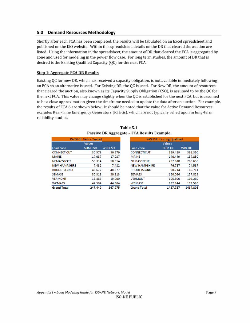
Step 1: Aggregate FCA DR Results

Existing QC for new DR, which has received a capacity obligation, is not available immediately following

an FCA so an alternative is used. For Existing DR, the QC is used. For New DR, the amount of resources

that cleared the auction, also known as its Capacity Supply Obligation (CSO), is assumed to be the QC for

the next FCA. This value may change slightly when the QC is established for the next FCA, but is assumed

to be a close approximation given the timeframe needed to update the data after an auction. For example,

the results of FCA 6 are shown below. It should be noted that the value for Active Demand Resources

excludes Real-Time Emergency Generators (RTEGs), which are not typically relied upon in long-term

reliability studies.

Table 5.1

Passive DR Aggregate – FCA Results Example


ISO-NE PUBLIC

Table 5.2

Active DR Aggregate – FCA Results Example

It should be noted in this example for this specific auction, two dispatch zones did not have any new

Active DR clear (Bangor Hydro and Springfield MA) and do not appear in the table on the left.

Step 2: Calculate Passive DRV by Load Zone

The next step is to sum the new and existing values of Passive DR for each load zone. Demand Resources

amounts in the FCA have the losses gross-up of 8% applied to make them equivalent to other capacity

resources on the system. To model the actual load reduction, or Demand Reduction Value (DRV), this 8%

gross-up needs to be removed. The values in the last two columns shown in the example below, illustrate

the DRV amounts that would be stored in the BCDB for use in the power flow model for the example

system.

Table 5.3

Passive DR Calculation by Load Zone Example


ISO-NE PUBLIC

Step 3: Calculate Active DRV by Dispatch Zone

Similar to passive DR, the existing and new Active DR (Excluding Real Time Emergency Generators) also

needs to be summed together and remove the losses gross-up used in the auction.

Table 5.4

Active DRV Calculation by Dispatch Zone Example

Step 4: Aggregate Forecasted EE Values from CELT Forecast

Starting in the 2012 CELT report, a new data column in the load forecast has been added, Summer

Passive Demand Resource (PDR). This value in the CELT report represents the cumulative PDR for an

area for the specified forecast year. Starting in year 5 of the forecast, the additional PDR represents the

forecasted EE. By taking the difference of year N and N+1 the incremental amount of forecasted EE can

be determined. Using the 2012 CELT report as an example, the following table represents the

incremental forecasted EE modeled in the CELT report.

Table 5.5 Forecasted EE from CELT Forecast by Load Zone Example


ISO-NE PUBLIC

Since these load values represent load & 8% losses, the losses need to be removed to represent the

forecasted EE DRV. The values in the next table shown in the example below represent the forecasted EE

DRV amounts that would be stored in the BCDB for use in the power flow model for the example system.

Table 5.6 Forecasted EE DRV Calculation by Load Zone Example

Step 5: Split DR Zone Totals by Substation

Now that the total amount of DRV is known for each zone (load or dispatch zone), it is divided up on the

substation level using the TO load distributions.

For example: Using the substations listed in the earlier example of Owner 456, assume that the Load Zone

A is made up of the 5 substations and that those stations are further split into Dispatch Zone B (East,

North, and Central) and Dispatch Zone C (South and West). After taking the DRV and increasing by 5.5%

to account for distribution losses, Load Zone A contains 50 MW of Passive DR and 10 MW of Forecasted

EE DR. Dispatch Zone B contains 15 MW of Active DR and Dispatch Zone C contains 10 MW of Active

DRV.


ISO-NE PUBLIC

Table 5.7 Owner 456 Substation DR Scaling Example

Substation Load Zone

Disp Zone

TO Provided Load Forecast

S/S Distribution (MW)

CELT Load (MW)

Passive DR

(MW)

Active DR

(MW)

Forecasted EE

(MW)

Net Load (MW)

East A B 100.00 97.59 -10.00 -5.00 -2.00 80.59

North A B 125.00 121.99 -12.50 -6.25 -2.50 100.74

Central A B 75.00 73.20 -7.50 -3.75 -1.50 60.45

Total Dispatch Zone B Modeled -15.00

West A C 50.00 48.80 -5.00 -2.50 -1.00 40.30

South A C 150.00 146.39 -15.00 -7.50 -3.00 120.89

Total Dispatch Zone C Modeled -10.00

Total Load Zone A DR Modeled -50.00 -10.00

Total Load 487.97 -50.00 -25.00 -10.00 402.97


ISO-NE PUBLIC

An example of how the Substation ‘South’ would be modeled in the power flow case is shown in Figure

5-1 and Table 5.8.

Figure 5-1: South Street Substation One-Line Diagram

Table 5.8 South Substation Load Records Example


ISO-NE PUBLIC

6.0 Load and Demand Resources Summary Reports

Each network model created for a study should be accompanied with a report describing how the load

was modeled. This section breaks down the report and gives a detailed description of each section.

Load Summary Report

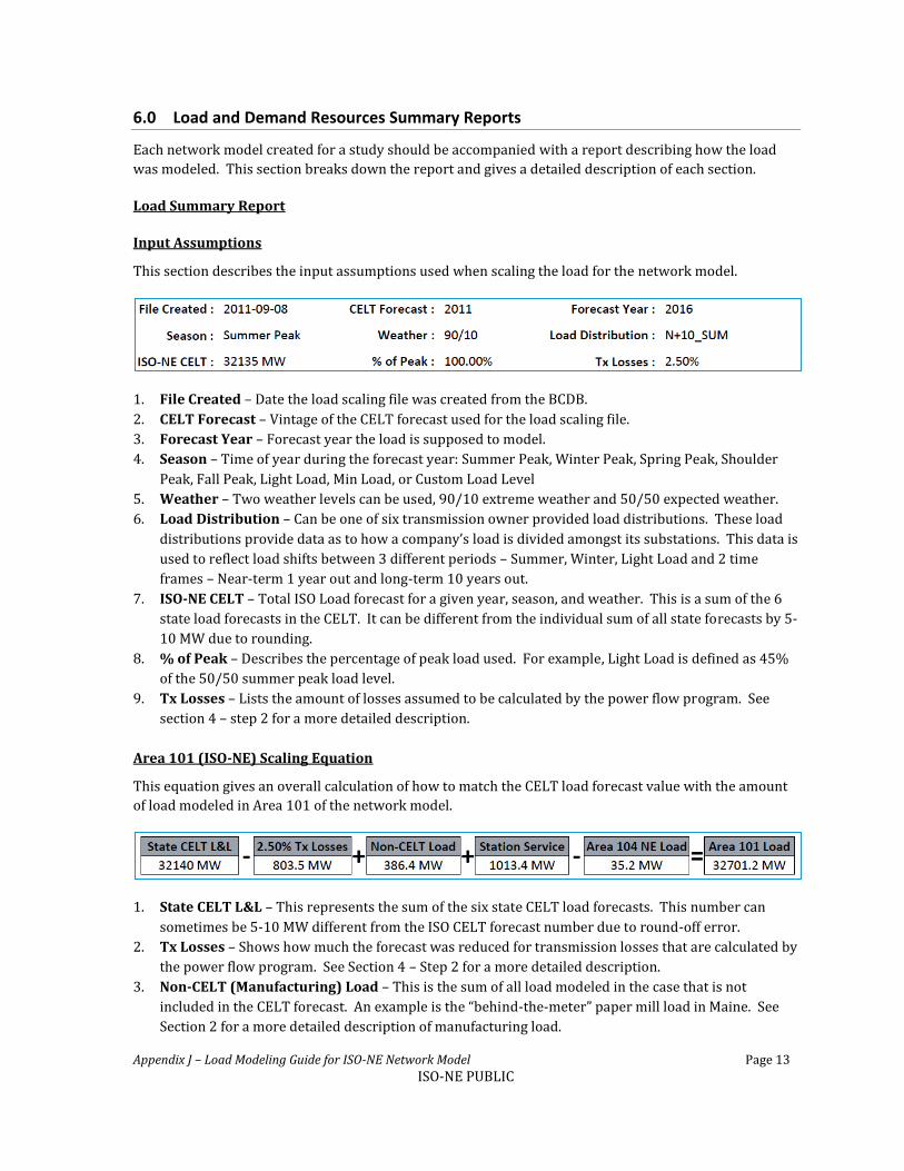
Input Assumptions

This section describes the input assumptions used when scaling the load for the network model.

1. File Created – Date the load scaling file was created from the BCDB.

2. CELT Forecast – Vintage of the CELT forecast used for the load scaling file.

3. Forecast Year – Forecast year the load is supposed to model.

4. Season – Time of year during the forecast year: Summer Peak, Winter Peak, Spring Peak, Shoulder

Peak, Fall Peak, Light Load, Min Load, or Custom Load Level

5. Weather – Two weather levels can be used, 90/10 extreme weather and 50/50 expected weather.

6. Load Distribution – Can be one of six transmission owner provided load distributions. These load

distributions provide data as to how a company’s load is divided amongst its substations. This data is

used to reflect load shifts between 3 different periods – Summer, Winter, Light Load and 2 time

frames – Near-term 1 year out and long-term 10 years out.

7. ISO-NE CELT – Total ISO Load forecast for a given year, season, and weather. This is a sum of the 6

state load forecasts in the CELT. It can be different from the individual sum of all state forecasts by 5-

10 MW due to rounding.

8. % of Peak – Describes the percentage of peak load used. For example, Light Load is defined as 45%

of the 50/50 summer peak load level.

9. Tx Losses – Lists the amount of losses assumed to be calculated by the power flow program. See

section 4 – step 2 for a more detailed description.

Area 101 (ISO-NE) Scaling Equation

This equation gives an overall calculation of how to match the CELT load forecast value with the amount

of load modeled in Area 101 of the network model.

1. State CELT L&L – This represents the sum of the six state CELT load forecasts. This number can

sometimes be 5-10 MW different from the ISO CELT forecast number due to round-off error.

2. Tx Losses – Shows how much the forecast was reduced for transmission losses that are calculated by

the power flow program. See Section 4 – Step 2 for a more detailed description.

3. Non-CELT (Manufacturing) Load – This is the sum of all load modeled in the case that is not

included in the CELT forecast. An example is the “behind-the-meter” paper mill load in Maine. See

Section 2 for a more detailed description of manufacturing load.


ISO-NE PUBLIC

4. Station Service – This is the amount of generator station service modeled. If station service is off-

line, the Area 101 report totals will be different since off-line load is not counted in totals.

5. Area 104 NE Load – This is load modeled in northern VT that is electrically served from Hydro

Quebec. To make Area Interchange load independent, this load is assigned Area 104.

6. Area 101 Load – After all these factors are applied to the original CELT forecast, this should be the

amount of load contained in Area 101 of the network model.

State Breakdown of Load Scaling – By Company

This section of the report describes how the state load forecast was broken down amongst the companies

within that state.

1. State – Lists the CELT load forecast for the state and what the load will be scaled to after

transmission losses are removed. See Section 4 – Step 2 for a more detailed description.

2. Company – This describes each company that is metered in the CELT report for the state.

3. State Share – This lists the percentage of the state forecast that each company will be scaled. See

Section 4 – Step 3 for a more detailed description.

4. Total P (MW) – This lists the amount of MW load for the company in the network model. It will

equal the state load minus transmission losses times the company’s state share.

5. Total Q (MVAR) – This lists the amount of MVAr load for the company in the network model. These

values are provided in the Transmission Owner load distribution data and the values are scaled

proportionally to the MW load to maintain the same power factor.

6. Overall PF – This is a calculation of the aggregate power factor for the company in the network

model. This value is just an overall average power factor for the Company. Each individual

substation may have different power factors depending on the data supplied by the TO.

7. Non-Scaling (MW) – This lists how much of the total MW load for the company is non-scaling CELT

load (described in Section 3).


ISO-NE PUBLIC

State Breakdown of Load Scaling – By Owner

This section of the report describes how the state load forecast was broken down amongst the owners

within that state.

1. State – Lists the CELT load forecast for the state and what the load will be scaled to after

transmission losses are removed. See Section 4 – Step 2 for a more detailed description.

2. Owner – Gives the owner number assigned to this load in the network model.

3. Description (Company) – A text description of the owner and it also lists the company that this

owner is represented in the CELT report for the state.

4. Total P (MW) – This lists the amount of MW load for the owner in the network model. This value

will match the report in the power flow model for the total load assigned to this owner.

5. Total Q (MVAR) – This lists the amount of MVAR load for the owner in the network model. These

values are provided in the Transmission Owner load distribution data and the values are scaled

proportionally to the MW load to maintain the same power factor.

6. Overall PF – This is a calculation of the aggregate power factor for the owner in the network model.

7. Non-Scaling (MW) – This lists how much of the total MW load for the owner is non-scaling CELT

load (described in Section 3).

Demand Resources Report

Input Assumptions

This section describes the input assumptions used when scaling the DR for the network model.

1. File Created – Date the DR file was created from the BCDB.

2. CCP – Capacity Commitment Period used for DR amounts. For example: CCP 2015/2016 represents

the DR cleared in Forward Capacity Auction (FCA) 6.

3. Load Season – Which CELT forecast year and time of year during that year. Used to determine de-

rate factors applied to DR described in the next section. Examples: Summer Peak, Winter Peak,

Spring Peak, Shoulder Peak, Fall Peak, Light Load, Min Load, or Custom Load Level

4. Load Distribution – Can be one of six transmission owner provided load distributions. These load

distributions provide data as to how a company’s load is divided amongst its substations. This data is


ISO-NE PUBLIC

used to reflect load shifts between 3 different periods – Summer, Winter, Light Load and 2 time

frames – Near-term 1 year out and long-term 10 years out.

5. Distrib Losses – Lists the amount of losses assumed to be from the customer meter where the DRV

is calculated to where the DR is modeled in the power flow. This value is described more in the next

section. Typically, the Transmission Losses (2.5% in this example) in the load file plus the

Distribution Losses (5.5% in this example) in the DR file should sum up to 8%.

6. DR Season – Either Summer or Winter. Depending on the Load Season, will determine which DR

capacity value to use. Winter DR is applied to winter peak and Summer DR is applied to all other

seasons.

Area 101 (ISO-NE) DR Scaling Equation

This equation gives an overall calculation of how to match the DR values from the FCA and forecasted EE

with the amount of DR modeled in Area 101 of the network model.

1. Demand Reduction Value (DRV) – Amount of DR measured at the customer meter without any

gross-up values for transmission or distribution losses.

2. Load Dependent Capability Assumption (LDCA) – De-rate factor applied based on % of CELT load.

(i.e. Light load is 45% of 50/50 load, so the LDCA would be 45%.)

3. Performance Assumption (PA) – De-rate factor applied based on expected performance of DR after

a dispatch signal from Operations.

4. Distribution Losses Gross-Up – This is the amount of losses that are added to the DRV. Since DR is

modeled at the low-side of the distribution transformer the net effect of the DRV at the customer

meter plus the amount losses reduced on the distribution network is modeled. This percentage is

typically based on 8% minus the amount of transmission losses assumed in the CELT load. For this

example we assumed 2.5% transmission losses, therefore 5.5% distribution losses are used.

5. Area 104 DR – This load is modeled in northern VT and is electrically served from Hydro Quebec. To

make Area Interchange load independent, this DR is assigned Area 104.

6. Area 101 DR – After all these factors are applied to the original DRV from the FCA, this should be the

amount of DR contained in Area 101 of the network model.


ISO-NE PUBLIC

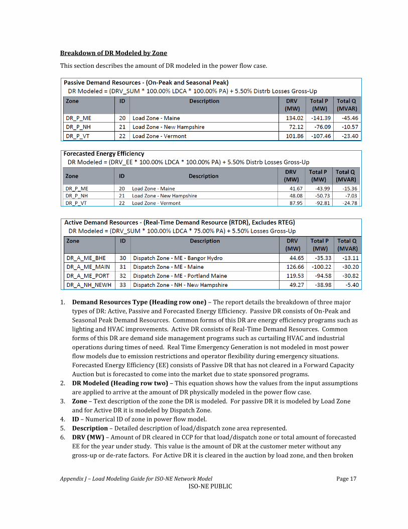
Breakdown of DR Modeled by Zone

This section describes the amount of DR modeled in the power flow case.

1. Demand Resources Type (Heading row one) – The report details the breakdown of three major

types of DR: Active, Passive and Forecasted Energy Efficiency. Passive DR consists of On-Peak and

Seasonal Peak Demand Resources. Common forms of this DR are energy efficiency programs such as

lighting and HVAC improvements. Active DR consists of Real-Time Demand Resources. Common

forms of this DR are demand side management programs such as curtailing HVAC and industrial

operations during times of need. Real Time Emergency Generation is not modeled in most power

flow models due to emission restrictions and operator flexibility during emergency situations.

Forecasted Energy Efficiency (EE) consists of Passive DR that has not cleared in a Forward Capacity

Auction but is forecasted to come into the market due to state sponsored programs.

2. DR Modeled (Heading row two) – This equation shows how the values from the input assumptions

are applied to arrive at the amount of DR physically modeled in the power flow case.

3. Zone – Text description of the zone the DR is modeled. For passive DR it is modeled by Load Zone

and for Active DR it is modeled by Dispatch Zone.

4. ID – Numerical ID of zone in power flow model.

5. Description – Detailed description of load/dispatch zone area represented.

6. DRV (MW) – Amount of DR cleared in CCP for that load/dispatch zone or total amount of forecasted

EE for the year under study. This value is the amount of DR at the customer meter without any

gross-up or de-rate factors. For Active DR it is cleared in the auction by load zone, and then broken


ISO-NE PUBLIC

down into dispatch zones proportional to the amount of CELT load in each dispatch zone. For an

example of how the DRV is calculated see Section 5.

7. Total P (MW) – Amount of real power DR modeled in the power flow case in each zone. This value is

derived from the base DRV with the gross-up and de-rate factors applied.

8. Total Q (MVAr) – Amount of reactive power DR modeled in the power flow case. The power factor

of DR is matched to the power factor of the load modeled at each bus.

7.0 Load and Demand Resources Reporting in Case Summaries

In many studies, a case summary script is used to display key characteristics of a power flow base case.

The ISO base case summary script includes a state-by-state breakdown of load and demand resources,

including scaling, non-scaling, station service, and non-CELT manufacturing load. A sample of this table is

provided below (numbers for illustrative purposes only).

The columns in the load summary each correspond to one of the types of load described in Section 3 of

this document, as follows:

1. Scaling Load – Scaling CELT Load

2. Non-Scaling – Non-Scaling CELT Load

3. Pass. DR – Passive Demand Resources

4. Act. DR – Active Demand Resources

5. Ener. Eff. – Forecasted Energy Efficiency (not including passive DR with FCM commitments)

6. Net Load – The net power delivered to customers included in the CELT forecast, equal to the sum of

scaling and non-scaling load, less passive DR, active DR, and energy efficiency.

7. Station Service – Generator Station Service Load

8. Non-CELT – Manufacturing Load not included in CELT forecast.

As with many load reports, totals may appear incorrect in the last decimal place due to rounding errors.

Also, please note that the sum of scaling and non-scaling load typically does not equal the CELT forecast.

This is due to the treatment of transmission system losses, which are included in the total load quoted in

the CELT forecast and discussed in Section 4 and explicit modeling of load and generation, which is

captured as net in the CELT forecast. The base case summary script does not include transmission system

losses, but simply quotes the sum of all loads modeled in the base case in each state listed.

transmission planning technical guide appendix j load ......the implementation of the model on...

Documents