TRANSPORTATION TRANSPORTATION PROBLEMPROBLEM

Shubhagata RoyShubhagata RoySchool of Management SciencesSchool of Management SciencesVaranasiVaranasi

Concept of Transportation ModelsConcept of Transportation Models

Transportation is a O.R. technique intended to Transportation is a O.R. technique intended to establish the ‘least cost route’ of transportation of establish the ‘least cost route’ of transportation of goods from the company’s factories to its goods from the company’s factories to its warehouses located at different places.warehouses located at different places.

It is a special type of linear programming problem It is a special type of linear programming problem (LPP) that involves transportation or physical (LPP) that involves transportation or physical distribution of goods and services from supply points distribution of goods and services from supply points (factories) to the demand points (warehouses). The (factories) to the demand points (warehouses). The problem involves determination of optimum routes to problem involves determination of optimum routes to minimize shipping costs from supply source to minimize shipping costs from supply source to destinations.destinations.

Let us assume that the company has three Factories Let us assume that the company has three Factories and four Warehouses. Our objective is to find the and four Warehouses. Our objective is to find the ‘least cost route’ of transportation. Let,‘least cost route’ of transportation. Let,CCijij= Unit cost of transportation from i= Unit cost of transportation from ithth factory to j factory to jthth warehousewarehouseXXijij= Quantity of the product transported from i= Quantity of the product transported from ithth factory to jfactory to jthth warehouse warehouse

FactoryWarehouse

Supply

1 2 3 4

1X11   X12   X13   X14  

a1

  C11   C12   C13   C14

2X21   X22   X23   X24  

a2

  C21   C22   C23   C24

3X31   X32   X33   X34  

a3

  C31   C32   C33   C34

Demand b1 b2 b3 b4 Total

Therefore the total cost of transportationTherefore the total cost of transportation

== XX1111.C.C1111+X+X1212.C.C1212+X+X1313.C.C1313+…………+X+…………+X3434.C.C3434

But since the objective is to minimize the total cost, But since the objective is to minimize the total cost, hence the objective function ishence the objective function is Min Min Z= XZ= X1111.C.C1111+X+X1212.C.C1212+X+X1313.C.C1313+…………+X+…………+X3434.C.C34 34

subject to supply constraintssubject to supply constraints,,

XX1111+X+X1212+X+X1313+X+X1414 = a = a11

XX2121+X+X2222+X+X2323+X+X2424 = a = a22

XX3131+X+X3232+X+X3333+X+X3434 = a = a33

demand constraints,demand constraints,XX1111+X+X2121+X+X3131 = b = b11

XX1212+X+X2222+X+X3232 = b = b22

XX1313+X+X2323+X+X3333 = b = b33

XX1414+X+X2424+X+X3434 = b = b44

Initial Basic Initial Basic Feasible SolutionFeasible Solution

1.1.North-West Corner Method North-West Corner Method (NWCM)(NWCM)

2.2.Least Cost Method (LCM)Least Cost Method (LCM)

3.3.Vogel’s Approximation Method Vogel’s Approximation Method (VAM)(VAM)

North-West Corner MethodNorth-West Corner Method

Step1: Select the upper left (north-west) cell of the transportation matrix and allocate minimum of supply and

demand, i.e., min.(a1,b1) value in that cell.Step2: • If a1< b1, then allocation made is equal to the supply

available at the first source (a1 in first row), then move vertically down to the cell (2,1).

• If a1> b1, then allocation made is equal to demand of the first destination (b1 in first column), then move horizontally to the cell (1,2).

• If a1=b1 , then allocate the value of a1 or b1 and then move to cell (2,2).

Step3: Continue the process until an allocation is made in the south-east corner cell of the transportation table.

ExampleExample:: Solve the Transportation Table to find Initial Solve the Transportation Table to find Initial Basic Feasible Solution using North-West Corner Method.Basic Feasible Solution using North-West Corner Method.

Total Cost =19*5+30*2+30*6+40*3+70*4+20*14Total Cost =19*5+30*2+30*6+40*3+70*4+20*14 = Rs. 1015 = Rs. 1015

Supply19 30 50 10

5 270 30 40 60

6 340 8 70 20

4 14Demand 34

S1

S2

S3

7

9

18

D1 D2 D3 D4

5 8 7 14

Least Cost MethodLeast Cost Method

Step1: Select the cell having lowest unit cost in the entire table and allocate the minimum of supply or demand values in that cell.

In case, the smallest unit cost is not unique, then select the cell where maximum allocation (allocation process will be same as discussed before) can be made.

Step2: Then eliminate the row or column in which supply or demand is exhausted. If both the supply and demand values are same, either of the row or column can be eliminated.

Step3: Repeat the process with next lowest unit cost and continue until the entire available supply at various sources and demand at various destinations is satisfied.

Supply

70

2

40

3Demand 345

S2 2

S3 3

D1

Supply

70 40 60

40 70 20

7Demand 34

S3 10

5 7 7

S2 9

D1 D3 D4

Supply

70 40

7

40 70

Demand 34

9

3S3

5 7

S2

D1 D3

Supply

19 30 50 10

70 30 40 60

40 8 70 20

8Demand 34

S3 18

5 8 7 14

S1 7

S2 9

D1 D2 D3 D4

Supply

19 50 10

7

70 40 60

40 70 20

Demand 34

7

9

S1

S2

S3 10

5

D1 D3 D4

7 14

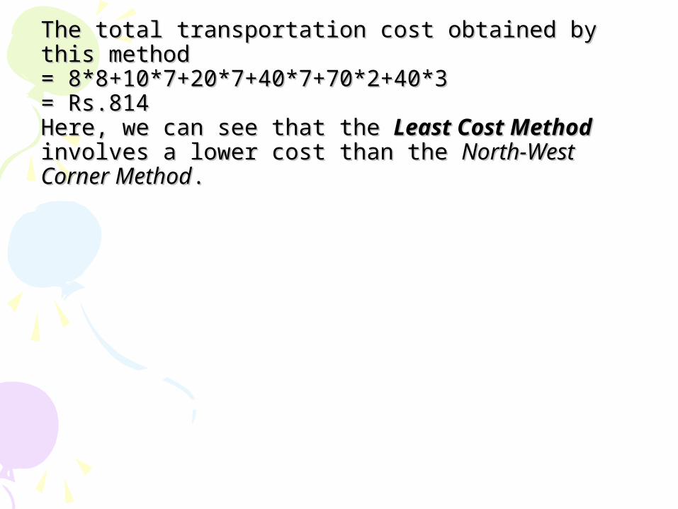
The total transportation cost obtained by this methodThe total transportation cost obtained by this method= 8*8+10*7+20*7+40*7+70*2+40*3= 8*8+10*7+20*7+40*7+70*2+40*3= Rs.814= Rs.814Here, we can see that the Here, we can see that the Least Cost MethodLeast Cost Method involves a involves a lower cost than the lower cost than the North-West Corner MethodNorth-West Corner Method..

Vogel’s Approximation MethodVogel’s Approximation Method

Step1: Calculate penalty for each row and column by taking the difference between the two smallest unit costs.

Step2: Select the row or column with the highest penalty and select the minimum unit cost of that row or column. Then, allocate the minimum of supply or demand values in that cell. If there is a tie, then select the cell where maximum allocation could be made.

Step3: Adjust the supply and demand and eliminate the satisfied row or column. If a row and column are satisfied simultaneously, only one of them is eliminated and the other one is assigned a zero value. Any row or column having zero supply or demand, can not be used in calculating future penalties.

Step4: Repeat the process until all the supply sources and demand destinations are satisfied.

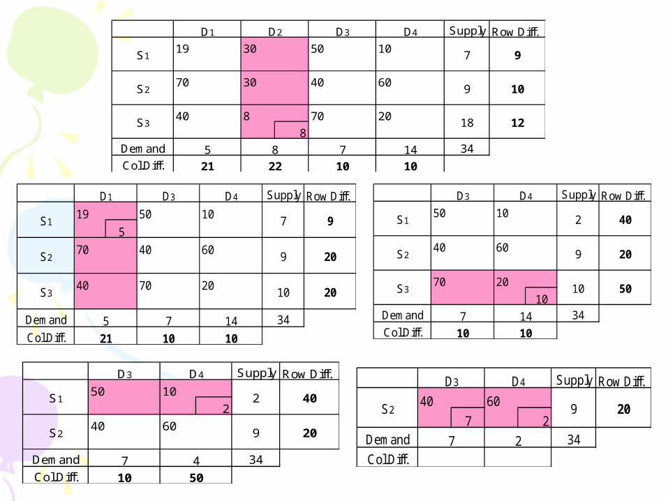
Supply Row Diff.

19 30 50 10

70 30 40 60

40 8 70 20

8Demand 34

Col.Diff.

9

10

12

21 22 10 10

D1 D2 D3

S1

S2

S3

5 8 7

D4

14

7

9

18

Supply Row Diff.

19 50 10

5

70 40 60

40 70 20

Demand 34

Col.Diff.

D1 D3 D4

S1 7

S2 9

S3 10

5 7 14

21 10 10

9

20

20

Supply Row Diff.

50 10

40 60

70 20

10Demand 34

Col.Diff. 10 10

40

20

50

D3 D4

S1 2

S2 9

S3 10

7 14

Supply Row Diff.

40 60

7 2Demand 34

Col.Diff.

20

7 2

S2 9

D3 D4Supply Row Diff.

50 10

2

40 60

Demand 34

Col.Diff.

20

10 50

40

7 4

S1 2

S2 9

D3 D4

The total transportation cost obtained by this methodThe total transportation cost obtained by this method= 8*8+19*5+20*10+10*2+40*7+60*2= 8*8+19*5+20*10+10*2+40*7+60*2= Rs.779= Rs.779Here, we can see that Here, we can see that Vogel’s Approximation MethodVogel’s Approximation Method involves the lowest cost than involves the lowest cost than North-West Corner MethodNorth-West Corner Method and and Least Cost MethodLeast Cost Method and hence is the most preferred and hence is the most preferred method of finding initial basic feasible solution.method of finding initial basic feasible solution.

Transportation Problem:Transportation Problem:

Moving towards OptimalityMoving towards Optimality

Once an initial solution is obtained, the next step is to Once an initial solution is obtained, the next step is to check its optimality. An optimal solution is one where check its optimality. An optimal solution is one where there is no other set of transportation routes there is no other set of transportation routes (allocations) that will further reduce the total (allocations) that will further reduce the total transportation cost. Thus, we have to evaluate each transportation cost. Thus, we have to evaluate each un-occupied cell in the transportation table in terms of un-occupied cell in the transportation table in terms of an opportunity of reducing total transportation cost.an opportunity of reducing total transportation cost.

If we have a B.F.S. consisting of (m+ n–1) independent If we have a B.F.S. consisting of (m+ n–1) independent positive allocations and a set of arbitrary number ui positive allocations and a set of arbitrary number ui and vj (i=1,2,...m; j=1,2,...n) such that cand vj (i=1,2,...m; j=1,2,...n) such that c ijij = u = uii+v+vjj for all for all occupied cells (i, j) then the evaluation dij occupied cells (i, j) then the evaluation dij corresponding to each empty cell (i, j) is given by :corresponding to each empty cell (i, j) is given by : d d ijij = c = cijij – (u – (uii+ v+ vjj))This evaluation is also called the opportunity cost for This evaluation is also called the opportunity cost for un-occupied cells.un-occupied cells.

Modified Distribution (MODI) or u-v Modified Distribution (MODI) or u-v MethodMethod

Step 1: Start with B.F.S. consisting of (m+ n–1) allocations in independent positions.

Step 2: Determine a set of m+n numbers ui (i=1,2,....m) and

vj (j=1,2,...n) for all the rows and columns such that for each occupied cell (i,j), the following condition is satisfied : Cij = ui+vj

Step 3: Calculate cell evaluations (opportunity cost) dij for each unoccupied cell (i,j) by using the formula :

dij = Cij – ( ui+vj ) for all i & j.

Step 4Step 4: : Examine the matrix of cell evaluation dij for Examine the matrix of cell evaluation dij for negativenegativeentries and conclude thatentries and conclude that(i) If all dij > 0 , then solution is optimal and unique.(i) If all dij > 0 , then solution is optimal and unique.(ii)If at least one dij = 0 , then solution is optimal and (ii)If at least one dij = 0 , then solution is optimal and alternatealternatesolution also exists.solution also exists.(iii)If at least one dij < 0 ,then solution is not optimal and an (iii)If at least one dij < 0 ,then solution is not optimal and an improved solution can be obtained.improved solution can be obtained.In this case, the un-occupied cell with the largest negative In this case, the un-occupied cell with the largest negative value of dij is considered for the new transportation value of dij is considered for the new transportation schedule.schedule. Step 5Step 5: : Construct aConstruct a closed path (loop) for the unoccupied closed path (loop) for the unoccupied cell having largest negative opportunity cost. Mark a (+) cell having largest negative opportunity cost. Mark a (+) sign in this cell and move along the rows (or columns) to sign in this cell and move along the rows (or columns) to find an occupied cell. Mark a (-) sign in this cell and find out find an occupied cell. Mark a (-) sign in this cell and find out another occupied cell. Repeat the process and mark the another occupied cell. Repeat the process and mark the occupied cells with (+) and (-) signs alternatively. Close the occupied cells with (+) and (-) signs alternatively. Close the path back to the selected unoccupied cell. path back to the selected unoccupied cell.

Step 6Step 6: : Select the smallest allocation amongst the Select the smallest allocation amongst the cells marked with (-) sign. Allocate this value to the cells marked with (-) sign. Allocate this value to the unoccupied cell of the loop and add and subtract it unoccupied cell of the loop and add and subtract it in the occupied cells as per their signs.in the occupied cells as per their signs.Thus an improved solution is obtained by Thus an improved solution is obtained by calculating the total transportation cost by this calculating the total transportation cost by this method.method.

Step 7Step 7: : Test the revised solution further for Test the revised solution further for optimality. The procedure terminates when all doptimality. The procedure terminates when all dijij ≥ ≥ 0 , for unoccupied cells.0 , for unoccupied cells.