truth and consequences of ordinal differences in

Psychological Bulletin1990, Vol. 108, No. 3, 551-567

Copyright 1990 by the American Psychological Association, Inc.0033-2909/90/$00.75

Truth and Consequences of Ordinal Differences in Statistical Distributions:Toward a Theory of Hierarchical Inference

James T. TownsendIndiana University

A theory is presented that establishes a dominance hierarchy of potential distinctions (order rela-tions) between two distributions. It is proposed that it is worthwhile for researchers to ascertain thestrongest possible distinction, because all weaker distinctions are logically implied. Implicationsof the theory for hypothesis testing, theory construction, and scales of measurement are consid-ered. Open problems for future research are outlined.

There are many occasions in psychological research whenexperimenters are concerned with two or more treatments andtheir effects on experimental groups. In most instances, themeasurements assessing the treatments are assumed to be on atleast an ordinal scale. The measurements typically form a sam-ple probability distribution. The investigator may then ask thequestion as to whether the two distributions differ from oneanother in some way. The way chosen is often through the test-ing of summary statistics, particularly sample means, but thereare techniques that test entire distributions against one an-other.

In this article I develop a theory that shows that some differ-ences between the distributions are stronger than others, inthat the stronger ones imply the weaker ones but not vice versa.In fact, a dominance hierarchy of distinctions between twoarbitrary distributions is developed: A distinction may implyanother, be implied by another, be equivalent to another, ornone of these. The dominance hierarchy is put into the form ofan implication graph. The power of the results is that they are,except for special cases to be specified later, general across dis-tributions. That is, most of the relations do not depend on aparticular type of distribution such as the normal distribution.Furthermore, as long as the measurements are on at least anordinal scale, again with the exception of the special cases, they

This research was supported by National Science Foundation Grant8710163 from the Memory and Cognitive Processes Section. I amgrateful to Robin Thomas and Trisha Van Zandt for help in prepara-tion of the figures, proofreading, and some theoretical calculations,and to Kilsoon Cummings and Katherine Fuller for typing the manu-script. Helpful comments were offered on an earlier version of themanuscript by Edna Loehman (Department of Agricultural Eco-nomics, Purdue University), David Moore (Department of Statistics,Purdue University), and Peter Schonemann, Hans Colonius, and Tri-sha Van Zandt (Department of Psychology, Purdue University). Tworeferees provided useful critiques. Certain of the present results werepresented at the nineteenth annual meeting of the Society for Mathe-matical Psychology at Harvard University, Cambridge, Massachusetts,August 1986.

Correspondence concerning this article should be addressed toJames T. Townsend, Department of Psychology, Indiana University,Bloomington, Indiana 47405.

are scale, and transformation-free up to a strictly monotonictransformation. Thus, in general the distinctions and implica-tions do not depend on interval or ratio level measurement, andinvestigators are free to perform useful monotonic transforma-tions on their data.

One immediate implication of the theory is that other thingsbeing equal, one can seek the strongest distinction reasonablein a given experimental context. Not only does this entail thetruth of the weaker distinctions, it also means that the experi-mental effect holds in a stronger sense. For instance, perhapsthe strongest distinction would be that every member (score,measurement, etc.) of the distribution under one treatmentwould be greater than every member of the distribution underthe alternate treatment. This is an extremely strong distinctionbut is, of course, rarely found in real studies. As I show, a morelikely possibility is that for each measurement or score, if thecumulative frequency (distribution function) of, say, Group A isalways higher than that of Group B at this score, then theseseveral other weaker distinctions, such as an ordering of themeans, are implied. In turn, this distributional ordering is im-plied by other even stronger distinctions.

Consider the situation in which an experimenter has admin-istered a psychological test to two groups, one presumablypathological and the other presumably "normal." It is possiblethat the frequency distributions of the test might differ in avery strong way, or they might differ in only a weak way. As asecond example, consider a situation in which the experimenteris examining performance through reaction time or- accuracy,when the subjects are under two different levels of informationprocessing load. The effect of the increased load on the under-lying processing mechanisms could be quite strong or, con-versely, might have a much weaker effect. Such consequencesmight be of importance not only in terms of the practical impli-cations for real-time performance, but also for their implica-tions with respect to potential theoretical explanations such asquantitative process models. Thus, the ramifications for thetype and degree of capacity limitation may hinge on the level atwhich the experimental distinction exists.

Let me expand on this general theme by developing in moredetail the idea of stronger versus weaker levels of distinctions.The technical notation is refined in the following paragraphs

551

552 JAMES T. TOWNSEND

and in the Appendix, but for now simply note that most of thediscussion refers to the population or ideal statistical concepts.Thus, the term distribution function is used for the populationcumulative frequency function and density is used for the popu-lation frequency function (which, for convenience and practical-ity, will be taken as being continuous in almost all cases). Whennecessary, "empirical" or "estimated" distributions or densitiescan be referred to as sampled approximations to the populationfunctions, but for the most part the "sampling" questions mustbe put aside.

Consider again the administration of the aforementioned psy-chological test to the two groups. Suppose that the investigatorentertains serious doubts about the satisfaction of the assump-tions of the normal (Gaussian) distribution by the underlyingpopulation distributions. In that case, the finding of a differ-ence in the means of the two groups could be quite weak interms of the dominance hierarchy. However, suppose it werefound that for any particular test score, there were always more"normals" who scored at that score or lower: That would be amore powerful finding than the one regarding a difference inthe means. The more powerful result is equivalent to the distri-bution function of the normal group always being greater thanthat of the presumed pathological group. This ordering of thedistribution functions in fact implies that the mean of the nor-mal group is less than that of the hypothetically pathologicalgroup. The implication here is invariant under monotonictransformations of the scores. Thus, if one is certain withinstatistical error that the distribution functions are ordered,then in principle there is no need to test the means. However,the means could be different without the distribution functionsbeing ordered. Thus the mean of the normals might be less thanthat of the pathological group, but for one or more particularscores, it might be that more of the pathological subjectsachieved a score that was less than or equal to that particularscore than was the case for the normal group. Hence, the dis-tinction between the two groups is less strong in this case.

It is true that certain types of distribution functions such asthe normal distribution, with equal standard deviations, havethe property that if there is a difference between the twomeans, then the distribution functions will also be ordered.However, it is rare in the behavioral sciences for the researchersto possess a high degree of confidence that all the assumptionsof normality are met in the underlying population distribution(see, e.g., Kendall & Stuart, 1973, Vol. 2, chap. 31; Mosteller &Tukey, 1977, chap. 1). Furthermore, I show how knowledge ofthis and other similar properties can aid theorists in their inves-tigations. I discuss the ramifications with regard to this ques-tion as well as that relating to the exact strength of the measure-ment scale later in the article.

Consider two other examples of how the type of results re-ported here might be of use in psychological investigations. Inthe first example, suppose a researcher has developed a mathe-matical model of how some response variable will change as afunction of an experimental variable. That model should thenpredict a distributional distinction at some level as the experi-mental variable is manipulated. Thus the researcher will likelywish to examine the data from the strongest level possible giventhe model. If it turns out that the distributions differ only at aweaker level, then this might call for a relaxation of certain

aspects of the model. These aspects might be of a purely techni-cal nature, or they may be more integrally related to the psycho-logical processes under investigation.

In the second example, which is in a sense an extension of thefirst, I consider the investigation of mental architecture in abehavioral experiment. By architecture I mean the way inwhich various psychological subprocesses may be connectedtogether. The simplest versions of a class of such architecturesare serial (i.e., the subprocesses are arranged sequentially) orparallel (i.e, the subprocesses are arranged so that they operatesimultaneously). More complex architectures can involve pro-cess interactions of considerable sophistication (Schweickert,1978). It is possible to identify the type of mental architecturethat is active in a particular cognitive task, if certain experimen-tal variables affect specific subprocesses (Townsend &Schweickert, 1989; Schweickert & Townsend, 1989). In most, ifnot all psychological tasks, the subprocesses must be assumedto be stochastic; that is, they take a random duration to operatefrom trial to trial. The question thus arises as to what aspect ofthe subprocesses' distribution an experimental variable mayaffect. The result is that if the experimental variable affects thatdistribution at a level of moderate strength within the domi-nance hierarchy, then even rather complex architectures can beidentified experimentally. These examples are amplified afterthe taxonomy is developed in more detail.

Before proceeding with that goal, I elaborate on certain fea-tures of the theoretical results. First, as was noted earlier, thescales of the underlying variate need only lie on an ordinalscale, although of course stronger scales are totally acceptable,as might be expected in such a situation. This may seem para-doxical because some results involve the arithmetic mean, andit is well known that many statements covering the mean aremeaningful in a measurement sense only if the scale is at leastinterval. The apparent paradox is explained and my perspectiveon the measurement background given in the section Level ofMeasurement Scale.'

Next, all of the relations between two distributions that willbe studied, with the exception of those pertaining to the nor-mal equal variance case, are distribution-free. They are alsoparameter free except in the trivial sense that the mean andmedian are thought of as parameters. Thus, except as noted, noparticular distribution or parameterization need be assumed touse these results. For some relations, statistical procedures areknown and available in standard sources. Cases in which thesehave apparently not been developed are pointed out. Perhapsresearch on these issues will be stimulated.

The presentation in this article is limited to single variates,for instance, scores, reaction times, and the like. However, itmay be possible to generalize the concepts to multivariate situa-tions by such devices as defining vector V to be greater thanvector W if and only if each entry of V is greater than the

1 Roberts and Marcus-Roberts (1987) observed that in certain situa-tions, as when a variable can attain only two possible values, even theordering of the means is invariant across monotonic transformations.They also noted the fact established by Lehmann (1955) that an order-ing of distribution functions implies an ordering of means. This rela-tion is discussed later.

HIERARCHICAL INFERENCE 553

Normal Equal Variance

Shift-Pair

fA(x) - fB(x-c)

c • constant > 0

L(x2)

THA(X)> tyx

for all x

F <x» F (x)A B

for all x

There are no densitycrossovers. Yet

- fA (X0) > fB(Xo)and fA(x) > fB(x)

if x<x0

MX)*fA(x) -

fA(x)

> fB(x) if x < x0

fB(x) > 0 if x • x0

< fB(x) if x > X,,

* *fA(x) crosses fB(x)

an odd number of times

Mean(XA)I

Med(XA)

Ip 'xAf XB' > 1/2

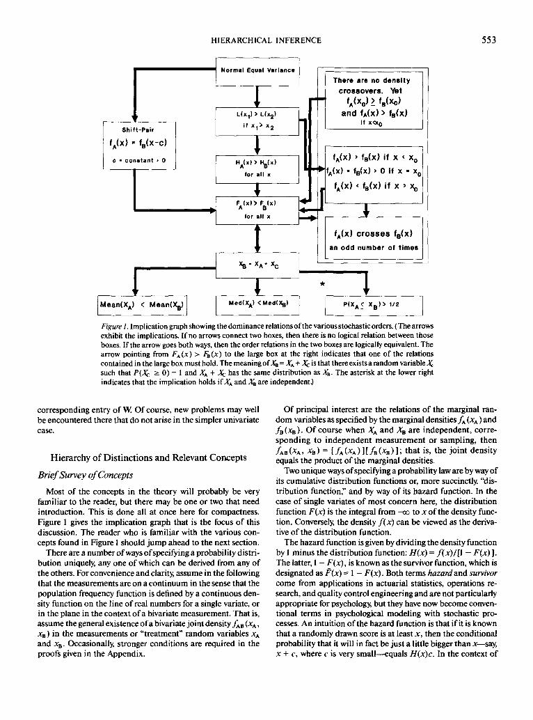
Figure 1. Implication graph showing the dominance relations of the various stochastic orders. (The arrowsexhibit the implications. If no arrows connect two boxes, then there is no logical relation between thoseboxes. If the arrow goes both ways, then the order relations in the two boxes are logically equivalent. Thearrow pointing from FA(x) > f^(x) to the large box at the right indicates that one of the relationscontained in the large box must hold. The meaning of X* = Xk + Xc is that there exists a random variable %such that P(Xc > 0) = 1 and X^ + Xc has the same distribution as X*. The asterisk at the lower rightindicates that the implication holds if A"A and AJ, are independent.)

corresponding entry of W. Of course, new problems may wellbe encountered there that do not arise in the simpler univariatecase.

Hierarchy of Distinctions and Relevant Concepts

Brief Survey of Concepts

Most of the concepts in the theory will probably be veryfamiliar to the reader, but there may be one or two that needintroduction. This is done all at once here for compactness.Figure 1 gives the implication graph that is the focus of thisdiscussion. The reader who is familiar with the various con-cepts found in Figure 1 should jump ahead to the next section.

There are a number of ways of specifying a probability distri-bution uniquely, any one of which can be derived from any ofthe others. For convenience and clarity, assume in the followingthat the measurements are on a continuum in the sense that thepopulation frequency function is denned by a continuous den-sity function on the line of real numbers for a single variate, orin the plane in the context of a bivariate measurement. That is,assume the general existence of a bivariate joint density fAV (XA ,XB ) in the measurements or "treatment" random variables XA

and XB. Occasionally, stronger conditions are required in theproofs given in the Appendix.

Of principal interest are the relations of the marginal ran-dom variables as specified by the marginal densities fA (XA ) and/B(XB)- Of course when XA and XE are independent, corre-sponding to independent measurement or sampling, then/AB(*A, *B) = [/A(*A) H/B(*B) ]; that is, the joint densityequals the product of the marginal densities.

Two unique ways of specifying a probability law are by way ofits cumulative distribution functions or, more succinctly, "dis-tribution function," and by way of its hazard function. In thecase of single variates of most concern here, the distributionfunction F(x) is the integral from -GO to x of the density func-tion. Conversely, the density f(x) can be viewed as the deriva-tive of the distribution function.

The hazard function is given by dividing the density functionby 1 minus the distribution function: H(x) = f(x)/[l - F(x) ].The latter, 1 - F(x), is known as the survivor function, which isdesignated as F(x) = I - F(x). Both terms hazard and survivorcome from applications in actuarial statistics, operations re-search, and quality control engineering and are not particularlyappropriate for psychology, but they have now become conven-tional terms in psychological modeling with stochastic pro-cesses. An intuition of the hazard function is that if it is knownthat a randomly drawn score is at least x, then the conditionalprobability that it will in fact be just a little bigger than x—say,x + c, where c is very small—equals H(x)c. In the context of


temporal phenomena, such as reaction time, it can be used torepresent the probability that processing will be completed inthe next instant, given that it has not been completed up untilthat time. The utility of the hazard function for actuarial statis-tics is evident. Life insurance companies are necessarily inter-ested in the probability that people born in a certain year willdie today (this year, etc.), given that they have survived untilnow. Similarly, quality control and maintenance engineers areconcerned with the probability that a product will fail pres-ently, conditioned on the event that it has lasted up until thepresent.

Other characteristics of probability laws, such as means andmedians, have proven indispensable in statistics, although aswill be shown, some of them convey much less informationthan others. Another important characteristic is the likelihoodratio, which simply is the ratio for any score x of the two densityfunctions under consideration. Let /A (x) be the density forTreatment A and /BW be the density for Treatment B; thenL(x) = AW//B(x) is the likelihood ratio as x ranges over itspossible values.

Hierarchy of Implication Graph

The dominance hierarchy of Figure 1 may be examined step-wise starting at the bottom with the mean and the median. Allthe propositions relating to Figure 1 are proven, or proofs arecited in the Appendix. Most of the relations hold even if themeasurements XA and XB are dependent; exceptions are noted.

Mean versus median. Beginning at the bottom of Figure 1, themean and median are seen under the assumption that Treat-ment B exceeds Treatment A, in the sense that the means ormedians are also ordered in that fashion. Interestingly, neitherthe mean nor the median bears implications for the other inthat either may be ordered in the manner shown and at thesame time the other may have the reverse order. It is natural thatthese hold no implications for one another because it is wellknown that they capture somewhat different aspects of the par-ent probability distribution.2

Figure 2a shows two theoretical densities that can be used toillustrate this and several other aspects of Figure 1. Figure 2bexhibits two empirically estimated densities from an experi-ment on short-term memory search. Proposition 1 in the Ap-pendix covers this case.

P(XA < X*). The function P(X^ < Xg) represents the proba-bility that the XK measurement is less than or equal to the XE

measurement. Thus, P(XA <Xv)>j says that Treatment B is atleast as large as Treatment A more than one half of the time. It israther surprising that this statement is probabilistically soweak, as is indicated in Figure 1. If XA and Xg are independent,then this ordering is implied by the higher entries in Figure 1,and with or without independence it does not even force themeans or medians to be ordered. Because ordering of themeans or medians also does not force P(XA < XE) > i, it followsthat all of these are logically unrelated to one another, and allare weaker than the other distinctions in the implication graph.The one exception is that if X^ and XB are dependent, then it ispossible to have FA(x) > FB(x) yet P(XA ^ XB) < 5, thus violat-ing the dominance structure depicted in Figure 1. Proposition2A treats the means and Proposition 2B the medians (see the

Appendix) with respect to the present type of stochastic order-ing. The theoretical example shown in Figure 2a yields P(X^ <,XE) = .75 to the second decimal. The empirical example ofFigure 2b has P(XA < Xg) = .82, approximately.

Adding a positive random variable and ordered distributionfunctions. The next entries in Figure 1 carry more force. Oneway to think about magnifying a set of measurements is to add anew positive random variable to the random variables repre-senting the original scores. Hence, one could produce a "larger"population, described by the random variable XB, by adding apositive random variable Xc to the "smaller" population de-scribed by XA; that is, set X^ = XA + Xc- A conceptually distinctbut, as it turns out, logically equivalent dominance relation isthe ordering of the two distribution functions FA (x) > Fs (x) forall x (except possibly where FA (x) and F^ (x) both equal 0 or 1).As is noted in the introduction of this article, this is interpretedas meaning that for any score or measurement x, the frequencyof those in Treatment A achieving x or lower is always largerthan those in Treatment B achieving x or lower. Proposition 3states that the two present dominance relations are equivalentin the sense that for any given distributional ordering, FA(JC) >FB (x), there exists a positive random variable Xc that can beadded to the random variable for Treatment A, X^, that willyield the distribution function of Treatment B and conversely.That is, XB= X^ + Xc. The random variable, Xc, may not beindependent of the random variable of Treatment A. Actually,for technical reasons, it is best to define a random variable X%with a distribution identical to that of X^ and then incrementX\. The details are covered in Proposition 3 in the Appendix.

In any event, a distributional ordering of two treatments is forpractical purposes the same as adding a possibly correlatedrandom variable to the larger of the two distributions (i.e., theone associated with the smaller scores).

Proposition 4A (see the Appendix) uses the FA(x) > FB(x)version to imply the ordering of the means and medians andwith the added assumption of independence also implies thatP(X^ < XB) > |, The reverse implications do not hold, soFA(x) > FB(x) and the equivalent XB = XK + Xc are trulystronger.

Proposition 4B indicates that without independence, thedominance of [FA(x) > f^(x) ] over [P(XA <, X^)> ^] may fail.An example in the Appendix confirms that one may find thatRunner A is faster than Runner B in that for every time t, theprobability that A beats that time is greater than the probabilitythat B beats that time (i.e, FA(t) > Ff(t)). Yet paradoxically, itmay be that Runner B defeats Runner A in over one half of theraces they run. The intuition for this and many other examplesis that in a majority of cases, A and B run (say) at about the samespeed and A always wins those races, leading toP(XA<,XB)<{.However, in some races, B is very fast, while A is very slow,leading to FA(x) < FB(x).

Figure 3a gives the distribution functions that correspond tothe Figure 2a densities, whereas Figure 3b shows the empirical

2 Another interesting sidelight is that there are situations, as withhigh-tailed distributions, in which the median may estimate the meanbetter than the arithmetic average of the data (e.g., Mosteller & Tukey,1977, chap. 14).


03o 0.500 -3

s- 0.400 :

m2 0.300 dQ

> 0.200 :

go.100 -

: 0.000 TI r^'Ti rrfffnTfTit 1 1 1 1 1 1 ] 11 nT'rn11 JTTT iiT r̂̂ ^Ti 11' 1 1 M |200 +00 600 800 1000 1200

TIME

200 400 600 800TIME

1000 1200

Figure 2. (a) Two population densities that are both logistic with thesame variance and different means; (b) two estimated densities replot-ted from data of Ashby (1982). (Ashby estimated them from a study byTownsend & Roos, 1973, on short-term memory search. The termfk(x) is the estimated reaction time density when the number of itemsin memory was 1, and fB(x) is that for five items in memory.)

distribution functions corresponding to Figure 2b, The "ideal"functions of Figure 3a indicate that they are ordered, and thesample functions of Figure 3b suggest that the data from whichthey are derived satisfy distributional ordering.

Density function crossings. The question arises as to how therespective density functions relate to the ordering of their dis-tributions. One interesting relation is found by studying theways in which the two density functions cross over one another.Figure 1 indicates that the distributional ordering, FA(x) >FE(x), implies that the density functions either must not crossat all or must cross an odd number of times. Conversely, if thenumber of crossings is 0 and the A density "gets started" beforethe B density, then FA(x) > f^(x). A special case of the latteroccurs when all of the A density lies to the left of the B density,an example of which was mentioned in the introduction of thisarticle. Furthermore, if the densities cross exactly one time, thedistribution functions are also ordered. However, an odd num-ber of crossings greater than 1 is compatible with a distribu-tional ordering but does not imply it. An immediate corollary isthat if fk (x) and fB (x) cross each other an even number of timesgreater than 1, then no distributional ordering is possible, andFA(x) and /fc(x) must cross.

Observe that because an odd number of crossings of the fre-quency functions might be accompanied by a distributionalordering, a single crossing of the frequency functions is strongerthan the distributional ordering and can be looked for in thedata with this in mind. Propositions 5 and 6 (see the Appendix)are relevant to these statements. The ideal densities shown inFigure 2a satisfy the single crossover point criterion, and theempirical cases in Figure 2b appear to do so also.

Shifting a distribution. A distinction that is definitelystronger than that of the ordering of distribution functions isthat of FB (x) = FA (x — c), where c is some positive constant.This immediately implies that FA(JC) > FB(x). That is, the dis-tribution functions are ordered if one is obtained from the otherby a shift of the measured variable. It is fairly evident, as shownby Proposition 7 (Appendix), that distribution functions canbe ordered without the strong assumption of shifting, so shift-ing is stronger and more constraining than simple distributionordering. The concept of creating a family of distributions bytaking an original distribution and performing arbitrary shiftson it is important in mathematical statistics.

Note that in Proposition 3, if the distribution on A^ is con-centrated, with all probability on one value X^ = C, we have theshift family. Interestingly, in the present case, the representation(by shift) is unique, whereas when Fc(xc) is nonnull, the repre-

200 400 600TIME

1000 1200

200 400 600 800TIME

1000

Figure 3. (a) F^(X) and F^(x) are the cumulative distribution func-tions associated with f^ (x) and /„ (x) of Figure 2a; (b) FA (x) and Fg (x)are the empirical distribution functions associated with the estimateddensities of Figure 2b.


senting additive random variable (and joint distribution) is ingeneral not unique.

For simplicity, the relation of shift pairs to density crossingshas been omitted in Figure 1. Basically, matters are inelegant inthe most general cases, in that weird shift-pair densities maycross an odd or even number of times. However, if /is unimo-dal by way of its derivative being positive for x less than themode and negative for x greater than the mode, then the twoshift densities cross exactly once. This is a strong manner ofgetting the distribution function ordering, which is shown inFigure 1. Note that fB(x) in Figure 2a is a shift of f * ( x ) . Theempirical densities of Figure 2b clearly do not satisfy this crite-rion.

Hazard functions. The next distinction is based on an order-ing for all x of the respective hazard functions. The first resulthere is that this ordering implies an ordering of the associateddistribution functions but not conversely, so that the ordering ofhazard functions is stronger than the ordering of distributionfunctions. This distinction, like the others, can be useful regard-less of the particular area of application. However, some maybe especially cogent in specific contexts. For instance, hazardfunctions carry considerable intuitive appeal when used in atime-dependent situation. When x represents time and HA (x) >/4M> the interpretation is that the instantaneous probabilityof finishing a task, given that it has not been completed up untiltime x, is always greater for Treatment A than for Treatment B.Because this distinction is stronger than an ordering of distri-bution functions, it follows that for all times x, the probabilitythat a Treatment A subject (a particular subprocess, etc.) is doneby time x, is always greater than that a Treatment B subject isdone by that time. Proposition 8 cites a proof of this finding(see the Appendix). It is important to note that an ordering oftwo hazard functions does not imply that either is itself a mono-tonic function of x. Figure 4a shows the ordered hazard func-tions associated with /A(x) and fv(x) of Figure 2a. Figure 4billustrates empirical hazard functions estimated in a rough wayfrom the densities of Figure 2b. Proposition 9 (Appendix)shows that a shift pair of distributions need not force theirhazard functions to be ordered, or vice versa. Proposition 10demonstrates that ordered hazard functions do not imply a sin-gle density crossover point (see the Appendix). Of course, ifthere is at least one crossover point, there there is an odd num-ber of crossovers, because otherwise the associated distributionfunctions would not be ordered.

Likelihood ratio. The next distinction, the likelihood ratio, isanalyzed because of its importance in statistical decisiontheory. It was surprising to learn that the assumption that thisfunction, defined as fA(x)//B(x), is monotonically decreasingis even more powerful than the ordering on hazard functions.The former implies the latter, but not vice versa as is shown inProposition 11 (see the Appendix). Intuitively, a monotonicallydecreasing likelihood ratio is saying that as one moves along theaxis of measurement, the evidence is always shifting continu-ously from Treatment A toward that of Treatment B. An exam-ple of its use in psychology is its application to signal detectiontheory (e.g, Green & Swets, 1966). There, as the decision crite-rion, figured as the likelihood ratio (equivalent to likelihoodfunction here), moves from minus infinity to plus infinity, it

0 020 -,2O

F 0-015 :

2D

0.010 H

0.005 H

0.000300

-m-prr400 500 600 700

TIME800 900 1000

0.040 -i

0.000300 400 500 600 700

TIME800 900 1000

Figure 4. (a) Hazard functions correspond to the probability distribu-tions from Figures 2a and 3a; (b) a rough estimate of the hazard func-tions corresponding to the empirical distributions of Figures 2b and3b. (It was not feasible to use the more sophisticated techniques ofBloxom, 1983.)

monotonically decreases (that theory typically uses the recipro-cal of my function so that Green and Swets' function increaseswhere the present function decreases) and in the process sweepsout the well-known receiver operator characteristic (ROC)curve. However, it is not typically used in that theory to distin-guish between distributions per se.

Proposition 12 suggests that for most usual cases, strictlydecreasing likelihood ratios imply a single density crossoverpoint. This proposition is stated loosely but appears to sufficefor present purposes. Proposition 13 gives an example showingthat a strictly decreasing likelihood ratio does not imply thatthe A and B densities are related by a shift.

Figure 5a demonstrates that L(x) for the example of Figure2a is monotonic in the proper manner. Figure 5b shows thelikelihood ratio generated by the empirical densities of Figure2b. It is intriguing that at least for the sizeable differences inprocessing load in Figures 2b, 3b, 4b, and 5b (one item vs. fiveitems in short-term memory) even the strongest distinction ofmonotonic likelihood ratio appears to hold. The hazard func-tions seem to lose their ordering for time greater than 900 ms,but that is in the extreme tail of the fK density. Certainly, cau-tion must be used here owing to the rough methods of estima-tion. Nevertheless, the example offers hope that at least in somecontexts, even the stronger distinctions may not be chimerical.


6.000 :

Q

§ 3.000 -

2 2.0003 1.000

0.000 _500 700

TIME900 1100

5.000 -i

P 4.000 :2Q 3.000 -Oo§ 2.000

a 1 .000

3

\ L i t )\\\\\

DO 500 700 900 1 1 00TIME

Figure 5. (a) L(t) is the likelihood function composed of the densitiesshown in Figure 2a; (b) L(t) is an estimate of the likelihood functiontaken from the estimated densities in Figure 2b.

Shift family of normal distributions. The strongest distinc-tion considered in this article is that of the shift family of nor-mal distributions; that is, the family of normal distributions forwhich the means may vary but the variances are the same orhomogeneous. As was previously noted, this obviously domi-nates the general shift family in the spirit of the hierarchy. More-over, along with the properties of the normal distribution fam-ily, all the other distinctions are implied. Thus, the likelihoodratio is monotonically decreasing, the hazard functions anddistribution functions are ordered, one distribution function isderived from the other by adding a constant to the first randomvariable (a special case of adding a new positive random vari-able to the first random variable), the one-point crossing prop-erty of densities holds, and so on. The proof of the strictlymonotonic likelihood ratio is given in Proposition 14. The factthat f^(x) and fB(x) are related by a shift is obvious; observethat the densities of Figure 2a are not normal, although theyprovide useful approximations to normal distributions. Theempirical densities of Figure Ib are decidedly not normal, as isthe case with most reaction time distributions. Observe that,like the ordering on means and shift pairs, the property ofnormality is not in general preserved under monotonic trans-formations.

A brief consideration of measurement and statistical issuesrelating to the hierarchy follows.

Implications and Issues ConcerningMeasurement and Statistics

Level of Measurement Scale

In this and the next section the implication graph in relationto the traditional question of discriminating between two treat-ment groups, conditions, or similar manipulations is discussed.The issue of the scale of measurement is intimately related tothe discrimination question. With provisos to be stated later,the properties of the implication graph hold regardless of thescale of measurement except the nominal scale, so that it isalways true that the higher up in the graph that a relation holds,the stronger the conclusions. Nevertheless, the ordinal proper-ties of the tree are of particular interest for psychology becauseof the difficulty in establishing scales at the interval or ratiolevel. The level of measurement issue is briefly dealt with, thenthe general problem of using the various orderings of the tree instatistical tests is discussed.

There is a long history of controversy about whether thestrength of the measurement—that is, nominal, ordinal, inter-val, or ratio—should affect the statistical operations that arevisited on one's data and on the investigator's conclusions. Thiscontroversy is not the main focus of the present research. Somerecent debates on the subject, which also include references toother contemporary and older works, are Davison and Sharma(1988), Gaito (1980), Michell (1986), Townsend and Ashby(1984). This article follows the foundational, or what Michell(1986) refers to as the representational, approach (e.g, Krantz,Luce, Suppes & Tversky, 1971; Narens, 1985; Pfanzagl, 1968;Stevens, 1951; Roberts, 1979; Suppes & Zinnes, 1963). This isnot the place for detail on a highly technical subject, but basi-cally this approach views a statistical statement as meaningfulif and only if the truth of the statement is invariant over admis-sible transformations of the scale.3 In the case of ordinal scales,the class of admissible transformations is that of strictly mono-tonic functions.

It should be noted that there are a number of technical condi-tions that must be satisfied to permit a qualitative probabilitydistribution to be defined on a relational system (see, e.g, Fish-burn & Roberts, 1989; Krantz et al, 1971, chap. 5; Van Lier,1989). It is the relational system that captures the regularity inempirical data that permit the mapping into a numerical repre-sentation. In fact, in most experiments, which naturally containonly a finite number of points, there is no definite way to assesseven the requirements of continuity of the scale (Pfanzagl,1968, pp. 76-79). Such conundrums appear to exist in allsciences, not just psychology. As in most cases of application ofmeasurement and probability, it is simply assumed here that theunderlying technical conditions are met, so that the appro-

3 Actually, matters can get rather Byzantine in the most generalcases (e.g., Roberts & Franke, 1976). However, suppose the scales areregular in the sense that if /and g are two scales for the same relationalsystem, then there is a transformation <t> such that g = <t>(f). Then thenotion of admissible transformation seems to adequately capture theidea of meaningfulness (see also Falmagne & Narens, 1983; Roberts,1979,1985).


priate scales and probability distributions on these scales arelegitimate. In this context, the reader may interpret "ordinalscale" to mean "ordinal scale with qualitative probability". An-cillary remarks are made on this subject in the Appendix.

One useful viewpoint in many psychological contexts is interms of a measured manifest variable that is itself a function ofa latent variable, the true object of interest to the psychologist.Now it is common in statistical inference to use (i.e., makestatements about) means in ways that demand interval levelmeasurement. For instance, most parametric tests such as Stu-dent's / test, multiple regression, and analysis of variance (AN-OVA), which likely make up the bulk of psychological applica-tions, rely on normal distributions. Linear (or affine) transfor-mations of normally distributed variables are again normal.Also, if two distributions have different means but the samevariance, then the ratio of the difference in means to the com-mon standard deviation remains invariant under affine trans-formations (i.e., y = ax + b, where a and b are constants).

These two properties cannot be overemphasized in terms oftheir importance for statistics. But the catch is that only mea-surements at the interval or ratio level are restricted to affine orlinear transformations (y= ax; i.e., b = 0 in the linear, specialcase of the affine representation). In particular, ordinal scalemeasurement permits any monotonic transformation, and thiswill enable any distribution, in particular the normal distribu-tion, to be perturbed to some other, often unspecified orunstudied, distribution. Thus, the manifest variable must bean affine function of the latent variable for the foregoing tech-niques to be meaningful in most circumstances. If it is onlyordinally related to the latent variable, it would seem nonsensi-cal to perform such tests. Furthermore, even if the manifest andlatent variables were one and the same, any strict monotonictransformation is still admissible.

In fact, it does seem likely that many psychological latentvariables lie at best on ordinal scales and thus carry only orderinformation. As such, they may legitimately undergo anymonotonic transformation, which to the adherents of the foun-dational (representational) view, effectively precludes the usualbattery of parametric analyses.4

Most of the orderings depicted in Figure 1 are invariantunder monotonic transformations. In other words, the class ofordered hazard functions is closed under that class of transfor-mations; so is the class of ordered distribution functions, and soon. However, as pointed out earlier, means do not necessarilystay ordered; furthermore, the shift family of distribution func-tions is not closed under monotonic transformations, althoughany such pair does remain ordered. Of course, the normal dis-tribution family is also not closed under monotonic transfor-mations.

Furthermore, some care must be taken with the entries relat-ing the distribution function ordering, FA (x) > FE (x) and X% =•*A + Xc- Recall that the distribution function ordering is logi-cally equivalent to adding a positive random variable to XA. Thedistribution function ordering is invariant under monotonictransformations of XA, X^ but of course, the distribution of Xc isexpected to change accordingly. Conversely, if XA and Xc arealtered monotonically, then the resulting Xe will be differentthan before the transformation was exacted. However, none ofthe logical implications in Figure 1 are harmed by these facts.

Within these guidelines, the implications of Figure 1 are notaltered by monotonic transformations, although as just noted,the particular entities satisfying a particular statement or rela-tion may change in the cases of two normally distributed vari-ables with equal variance, a shift pair and a pair of orderedmeans. Overall then, and with these caveats, as long as thelatent variable and the manifest variable are monotonically re-lated, the relations of Figure 1 continue to hold if they heldbefore the transformation and fail to hold if they violated therelation before the transformation.

Davison and Sharma (1988) have pointed out that if the den-sities cross exactly once, then ordered means stay ordered.Thus, if the latent and manifest variables are monotonicallyrelated, then the means of both must be ordered in the sameway. The dominance hierarchy of Figure 1 shows that the singlecrossover condition is even stronger, in that the distributionfunctions themselves stay ordered in going from the manifest tothe latent variable. The latter in turn produces the mean order-ing developed by Davison and Sharma, as is shown in Figure 1.

Davison and Sharma (1988) also noted that the example usedby Townsend and Ashby (1984) does not satisfy the single cross-over condition, and hence the order of the means need not bepreserved under a monotonic transformation. Actually, in thatexample the difference in the means in relation to the appro-priate variance was enlarged from 0 to an arbitrary number,hence an arbitrary level of significance, but their basic pointremains valid. From a purist's viewpoint, it is in any case mean-ingless to speak of "statistical significance" when the normaldistribution is only one of an infinite number of distributionsthat applies to this situation. Also, in general, two arbitrarydistributions cannot be changed to both be normal through asingle transformation, so that one may not somehow refer to anormal "canonical" form for two such distributions in order toprovide for a statistical test.

From the opposite direction, what if a set of measurements ison an interval or ratio scale? For instance, when used in itsphysical sense rather than as a measure of a psychological vari-able, reaction time may lie on a ratio scale (cf. Krantz, 1972;Micko, 1969; Townsend, in press; Townsend & Ashby, 1983, pp.387-390).5 As has been noted, reaction time data are almost

4 As was rightly pointed out by a referee, an analysis may not be ruledout simply because it is parametric. Suppose that a statement, for in-stance one involving a comparison of two distributions, is based on aparameter of the assumed family of distributions and that the truth ofthis statement is invariant under all strictly monotonic transforma-tions. Then it follows that one has a legitimate ordinal comparison thatnevertheless is "parametric." However, it is a fact that most common-place statistical tests do not satisfy the foregoing condition but ratherdemand at least interval level measurement.

5 A referee pointed out that not all investigators believe that reactiontime lies on a ratio scale and cited Krantz (1972) in this regard. Thisissue obviously cannot be dealt with in detail here. Elsewhere, I arguethat processing time consumed by a psychological mechanism (whichultimately refers to action by a congeries of neural elements) can incertain cases be treated exactly as if one were measuring the fall-timeof an apple from a tree (Townsend, in press). The reaction time scalewould then be ratio in such contexts. On the other hand, if reactiontime, or virtually any other dependent variable, is taken as a measureof a psychological entity, such as response strength in Krantz (1972),


never normal in appearance, but rather positively skewed. If thescale is ratio, it is illegitimate to transform the scale or data inorder to render the distribution more normal in form. Thus,the investigator must develop parametric tests that are specificto a family of distributions that seem to match the sample fre-quency functions, or they must use distribution-free tests (seethe next section). The latter may be in some cases the better andmore efficient approach.

Statistical Analyses

Nonparametric statistics treats estimation and hypothesistesting in such a way that the specific parameters of a distribu-tion may be safely ignored. Distribution-free statistics relaxesthings further in that even the form of the distribution can beneglected. Thus, distribution-free implies parameter-free, butnot conversely. As was noted earlier, except insofar as, say, themean is considered to be a parameter of a distribution, thepresent methodology is both distribution- and parameter-free.By convention, nonparametric or parametric-free tests are of-ten also distribution-free. (But see Kendall & Stuart, 1973, Vol.2, for a discussion of this issue.)

Presently, there seems to be no theoretical structure existingin the field of statistical hypothesis testing corresponding tothe present hierarchy as a whole. The implication graph of Fig-ure 1 originally grew out of questions related to the strength ofcognitive capacity limitations as revealed through reaction timestatistics (e.g., Townsend, 1974; Townsend & Ashby, 1978).That is, the mental work load is varied, and some statistic orfunction is used to assess the effects on reaction time. All of thepropositions relating to Figure 1 (see the Appendix) have beenproven independently by myself and my associates. However,we subsequently uncovered lines of research in other domainsin which stochastic orders have proven of importance. Earlyrelated papers are Rubin (1951) and Lehmann (1955). Stochas-tic orders are related to the concept of majorization, which pro-vides a general approach to the study of probabilistic domi-nance relations (see, e.g, Marshall & Olkin, 1979). A readablebeginning source for other approaches and applications outsidepsychology of some of the orders of Figure 1 is Ross (1983),which also includes additional references.

There are statistical procedures for some of the distinctionsdisplayed in Figure 1, but several distinctions lack such meth-ods. In addition, whereas some of the distinctions may betested without recourse to estimation, in other cases, estima-tion procedures must be carried out before asking whether thedistinction holds in the investigator's data. (This seems an aptplace to remind the reader about the danger of a inflation thatmay accrue with a series of statistical tests.) Finally, there seemsto be little known about the general relation of statistical powerto the dominance hierarchy of relations, which is presentedbelow. It is also important topic for further research.

Several of the relations of Figure 1 are illustrated by data from

then one must proceed to obey the tenets of foundational measure-ment in order to establish the scale type. Finally, it is not obvious thatthis assertion or its contrary is subject to logical proof. Perhaps arguingby analogy to theory and measurement in other sciences is as close asone can come.

the experimental literature. It is convenient to begin this time atthe top of Figure 1, where the strongest distinctions reside. Theshift family of normal distributions (i.e, equal variance, butpossible unequal means) is the cornerstone for much of para-metric statistics, either directly, as in the z test or ANOVA, orbecause it enters into other theoretical formulae or derivations,as in the t test or central chi-square distribution.6 If the modelitself is true, then all the major distinctions of Figure 1 are inforce (see the previous section for caveats).

The left side of Figure 1 shows fA(x) and /B(JC) related by ashift transformation. Nonnormal shift families of distributionsare popular in theoretical work in statistics, and it happilyturns out that there is a test of the hypothesis that f^ is a shiftedversion of FA. It appears in Pitman (1938) and is discussed byKendall and Stuart (1973, Vol. 2, pp. 505-510).

Next, the likelihood ratio being used, appearing seconddown in the center of Figure 1, should not be confused with thelikelihood function used in the so-called likelihood ratio test(e.g, Wilks, 1962, p. 402) that provides for a test of compositehypotheses by using a ratio of densities based on a null hypothe-sis versus a broader based hypothesis (e.g, testing a specificvalue of a mean vs. any positive mean). There are mathematicalrelations between the latter conception and mine, but these arebeyond the present scope of this article. As far as is known,there are no available tests that directly assay whether the likeli-hood ratio is monotonically decreasing. Probably it would benecessary to estimate the density functions first before evaluat-ing the performance of the function as the variate or scoresincrease. Even then, there appears to be no test available tostatistically evaluate that question. Thus, at this time, this verypowerful distinction apparently must be evaluated in a qualita-tive and statistically inexact fashion. One might use proceduresto estimate the density functions in a distribution-free way (seethe discussion on estimation at the end of this section) and thenobserve the results with an eye to looking for obvious or ex-treme violations of monotonicity of the likelihood function.

The state of the art with regard to hazard functions is also lessthan what one might hope, although here, too, progress hasbeen made, at least with regard to estimation of the underlyinghazard functions under, say, two conditions. However, againthere appear to be no known procedures for statistically evaluat-ing the order of the two functions. For that one requires either adistribution-free theory, corresponding to what exists in thecase of distribution function ordering (see the following sec-tion) , or a derivation of sampling distributions of the samplehazard functions, based on underlying parametric distribu-tions. Nevertheless, there are early indications that empiricalsituations in psychology exist for which the hazard functionsare indeed ordered; this will be seen in the next section.

The question of where and how many times two densitiescross also has apparently not received great attention from stat-isticians. From a somewhat different viewpoint, the issue ofwhere they cross has been shown to be of theoretical interest byAshby (1982) and Ratcliff (1988) in cognitive and perceptual

6 Recall that the central chi-square distribution may be derived asthe sum of a set of normally distributed random variables, each with amean equal to zero and a standard deviation equal to 1.


search experiments. Thus, it may be that interest can be pro-voked in several arenas that will encourage more attention tothis problem.

Matters improve again with the distribution function order-ing FA(JC) > Fs(x). Here one can rely on the well-known Kol-mogorov-Smirnov test (Kendall & Stuart, 1973, pp. 473-476;Siegel, 1956, pp. 127-136). The basic two-sided test simply de-cides whether two distribution functions are the same. If thenull hypothesis of equality is rejected, then one may proceed toa one-sided test with the null hypothesis being that FA > FB. Ifthe latter is accepted, one has the "predicted" ordering. If theone-sided null hypothesis is rejected, one infers that either atrue crossover of the distribution functions exists or that theordering goes in the opposite direction. The last possibility canbe checked by another one-sided test.

There appear to be no statistical tests that address the ques-tion of whether a given distribution function can be repre-sented as being generated by the random variable of anotherdistribution plus an added positive random variable. However,as can be seen from Figure 1, the distribution function orderinglogically implies the existence of such a random variable, andvice versa, so the appropriate tests for the former can also beused with the latter.

Because means can be reordered by monotonic transforma-tions, there can be no ordinal tests involving them. However,there are a number of tests for the medians (see, e.g., Kendall &Stuart, 1973, Vol. 2, chap. 12, orSiegel, 1956, pp. 111-116). Thestatement that P(XA <XB)>{ forms a composite one-tail alter-native to the null hypothesis that P(X^ < XB) = \. This isreadily assessed by the well-known sign test (e.g., Siegel, 1956,pp. 68-75).

Several of these orderings, such as number of density cross-ings and monotonicity of the likelihood function, may dependon adequate estimation of the densities or other functions, suchas the hazard function. It may be surprising that although f ( x ) ,F(x), and H(x) all yield total information about a distribution,a good estimate (e.g, optimal in some sense) of one of themdoes not necessarily lead to a good estimate of the others. Forinstance, the empirical distribution function proves to be agood estimate of the population distribution function yet doesnot immediately lead to an adequate estimate of the densityfunction representation. The distribution function F has beenmost studied, and the situation for the Kolmogorov-Smirnovtest is simplicity itself because the test is accomplished on thetwo usual cumulative frequency functions (also known as thecumulative step function and the empirical distribution functionamong other less well-known titles). This is easily obtained,and no difficult estimation problems intercede (for more detailsee Wilks, 1962, pp. 454-459).

Matters are not so complete in the case of the density andhazard functions, but densities have occupied a good deal ofattention from statisticians, engineers, and quantitative psychol-ogists in recent years and hazard functions somewhat less of-ten. Psychologists might begin with some recent papers ofBloxom (1983, 1984, 1985). Bloxom provided his own ap-proach both to densities and hazard functions but also aidedthe reader in accessing the general literature on these topics.Furthermore, some of his techniques are especially importantfor the process theorist because they view a particular distribu-

tion as being a component in an overall processing system (as inserial, parallel, etc.).

Theoretical Applications

By theoretical applications, I refer to applications whose mainintent is other than the immediate discrimination between twoexperimental treatments, in the broad sense. Thus, included inthis section is the problem of discerning how alteration of adistribution, for instance, through change of a parameter, willaffect theoretical predictions. For example, suppose it is postu-lated that an experimental manipulation affects a certain pa-rameter of a distribution in a psychological model of the experi-mental task. That distribution, then, as part of the model, willproduce a prediction that may fall into an ordering of the typepictured in Figure 1. In many such cases, one can then referback to the previous section for points relating to the appro-priate statistical tests and other pertinent information. There isanother more subtle way in which the implication graph can beused that is discussed subsequently.

An example of a distribution function ordering was given byTownsend and Ashby (1983, pp. 210-211), who showed thatindependent serial processes and independent parallel pro-cesses both predict distribution function orderings as the num-ber of items to process increases (see also Lupker & Theios,1977; Sternberg, 1973; Vorberg, 1981). Therefore both serialand parallel models can predict the distribution ordering ofreaction times found in a reanalysis of the Townsend and Roos(1973) study on memory and visual display search, referred toin an earlier section. Figure 3b is an example of the results. Thereader is referred to Townsend and Ashby (1983, chap. 8) forrelated issues and tests.

Townsend and Ashby (1983, pp. 272-289) applied some ofthe results of the present article to a parallel horse race modelbased on two parallel counters (also called accumulators). Con-sider an application to a pattern classification experiment inwhich the subject must respond as to which of two classes astimulus pattern belongs. Suppose that the correct counter al-ways counts at a faster rate than the incorrect counter. Then ifthe criterion number of counts for the correct counter to "de-tect" is less than or equal to that for the incorrect counter, theconditional distribution function of the correct counter willalways be greater than that for the incorrect (error) counter, sayFc(t) > Fc(t). It immediately follows that the average correctresponse times must be faster than error response times. Fur-thermore, when both are running in parallel, the correctcounter will beat the incorrect counter to a detect responsemore than one half of the time, corresponding to a probabilitycorrect greater than one half. The latter is, of course, a distribu-tion-free prediction corresponding to P(Xk < X^) > {in Figure1. This type of theoretical analysis already seems to be provingof value in testing competing models of two-choice discrimina-tion (e.g., Smith & Vickers, 1988).

Busemeyer and his colleagues have used stochastic domi-nance orderings in obtaining predictions. They have found, aswe have, that sometimes the stronger level is actually the easierto prove. Thus, in Busemeyer, Forsyth, and Nozawa's (1988)theoretical comparison of two dynamic choice models, it wasshown that a likelihood function was monotonic in order to


prove the ordering of two theoretical means. In another in-stance, Busemeyer and Rapoport (1988) argued from the em-pirical finding of a crossing of two distribution functions that acertain model that predicted that an ordering would occurmust be wrong.

Burbeck and Luce (1982) were not directly testing treatmentdifferences using the Figure 1 hierarchy, but some of their re-sults are interesting from that perspective. Seven of the nineestimated hazard function pairs, one for the less intense toneand one for the more intense tone, appear to be ordered (Bur-beck & Luce, 1982, Figure 5). From the implication graph inFigure 1, it can be seen that strong consequences ensue in termsof the speed of completion of the underlying detection processunder the two conditions. It is also interesting that one of theirplausible single process models, which turned out not to fit sowell, clearly fails the hazard function ordering as a function ofits shape parameter (see Burbeck & Luce, 1982, Figure 6).

In a study on pain tolerance, Stevenson, Kanfer, and Higgins(1984) manipulated goal and cue information, regarding thetime remaining or time elapsed of the pain stimulus. Amongother effects was the finding that the empirical distributionfunction of termination in the cue-to-cue interval was greaterfor the cued than for the uncued subjects. This result was inter-preted to indicate that the cued subjects, given that they had notyet stopped at the point of a cue, tended to quit earlier in theinterval before the next cue than did the control group. Thus,the cues may have served as psychological epoch markers asmuch as motivators to remain in pain longer overall.

The idea of stochastic ordering has played an important rolein certain research areas of economics and decision making.Two starting references here are Hadar and Russell (1969) andBrumelle and Vickson (1975).

The final example extends the prediction concept. Schweick-ert and Townsend (Schweickert & Townsend, 1989; Townsend& Schweickert, 1985; Townsend & Schweickert, 1989) have de-veloped a method of identifying mental architecture within abroad class of mental networks (directed acyclic networks en-dowed with probability distributions on the durations con-sumed by the subprocesses; see, e.g, Fisher & Goldstein, 1983;Schweickert, 1978). A key feature is that internal subprocessesare experimentally affected by way of incrementing their pro-cessing time random variables. This incrementing conforms tothe addition of a positive random variable as is seen in Figure 1and therefore is at the same level of strength as a distributionfunction ordering. When two subprocesses are so manipulated,it is possible to determine the type of architecture in which thetwo subprocesses are embedded, by observations at the level ofoverall mean reaction times.

Summary and Conclusions

A theory of hierarchical inference was developed and a graphthat exhibits the implication relations among the consequentset of order relations has been presented in Figure 1. The impli-cation graph shows that there is a hierarchy of strength holdingamong various individual indices of ordering. The form of theranking of one treatment over another frequently was in termsof an ordering of two statistics or functions, although in certaincases, density crosses or shifts of a distribution created ordering

relations. It is proposed that it is to the advantage of an experi-menter to determine the strongest way in which one treatmentgroup diners from another, for instance, as an ordering of thedistribution functions instead of simply a difference in themeans. The ordering relations in Figure 1 where statistical testsexist are pointed out as well as certain references to literature onassociated estimation problems. It is not possible to develop ordiscuss sample and estimation themes in detail. I hope that thepotential utility of these and similar dominance relations willencourage statistical theorists and psychologists to develop fur-ther hypothesis tests based on them.

For those who hold the level of measurement (ratio vs. inter-val vs. ordinal) to be important in the application of statistics,the invariance of the Figure 1 relations (a form of statisticalstatement) under monotonic transformations could be an im-portant advantage, along with other distribution-free statisticalprocedures. It has been further shown that the relations of theimplication graph could be helpful in theoretical investiga-tions, particularly in assessing the level at which a model ortheory would predict a difference between two treatments (asproduced through manipulation of a theoretical distribution).Such results tell researchers at what level they should expect todetect experimental differences. Also, a difference on this di-mension between two models may itself indicate a testable dis-tinction or, other things being equal, suggest that a model pre-dicting the stronger difference, in terms of Figure 1, is the pre-ferred model because it is more falsifiable. Finally, a way ofusing the method to identify internal cognitive processing ar-chitecture has been discussed. Several examples of use of theconcepts, some hypothetical and some from the psychologicalliterature, have been offered. Most of them were from the per-ceptual and cognitive literature because that is the domain ofthis author. I hope that those from other areas will find theproposed theory of value.

References

Ashby, F. G. (1982). Testing the assumptions of exponential additivereaction time models. Memory and Cognition, 10,125-134.

Bloxom, B. (1983). Some problems in estimating response time distri-butions. In H. Wainer & S. Messick (Eds.), Principles of psychologi-cal measurement: A Festschrift in honor of Fredrick M. Lord. Hills-dale, NJ: Erlbaum.

Bloxom, B. (1984). Estimating response time hazard functions: Anexposition and an extension. Journal of Mathematical Psychology,28, 401-420.

Bloxom, B. (1985). A constrained spline estimator of a hazard func-tion. Psychometrica, 50, 301-321.

Brumelle, S. L, & Vickson, R. G. (1975). An unified approach tostochastic dominance. In W Ziemba & R. G. Vickson (Eds.), Sto-chastic optimization models in finance. New York: Academic Press.

Burbeck, S. L_ & Luce, R. D. (1982). Evidence from auditory simplereaction times for both change and level detectors. Perception andPsychophysics, 32,117-133.

Busemeyer, J. R., Forsyth, B., & Nozawa, G. (1988). Comparisons ofelimination by aspects and suppression of aspects choice modelsbased on choice response time. Journal of Mathematical Psychology,32, 341-349.

Busemeyer, J. R., & Rapoport, A. (1988). Psychological theory of de-ferred decision making. Journal of Mathematical Psychology, 32,91-135.


Chung, K. L. (1974). A course in probability theory. San Diego, CA:Academic Press.

Davison, M. L., & Sharma, A. R. (1988). Parametric statistics andlevels of measurement. Psychological Bulletin, 104,137-144.

Falmagne, J. C, & Narens, L. (1983). Scales and meaningfulness ofquantitative laws. Synthesis, 55, 287-325.

Fishburn, P. C., & Roberts, F. S. (1989). Axioms for unique subjectiveprobability on finite sets. Journal of Mathematical Psychology, 33,117-130.

Fisher, D. L., & Goldstein, W M. (1983). Stochastic PERT networks asmodels of cognition: Derivation of the mean, variance, and distribu-tion of reaction time using order-of-processing space (OP) dia-grams. Journal of Mathematical Psychology, 27,121-151.

Gaito, J. (1980). Measurement scales and statistics: Resurgence of anold misconception. Psychological Bulletin, 87, 564-567.

Green D. M., & Swets, J. A. (1966). Signal detection theory and psycho-physics. New York: Wiley.

Hadar, J., & Russell, W R. (1969). Rules for ordering uncertain pros-pects. American Economic Reviews, 59, 25-54.

Kendall, M. G., & Stuart, A. (1973). The advanced theory of statistics(Vol. 2). New York: Hafner.

Krantz, D. H. (1972). Measurement structure and psychological laws.Science, 175,1427-1435.

Krantz, D. H., Luce, R. D, Suppes, P., & Tversky, A. (1971). Founda-tions of measurement (Vol. 1). New York: Academic Press.

Lehmann, E. L. (1955). Ordered families of distributions. Annals ofMathematical Statistics, 26, 399-419.

Lupker, S. J., & Theios, J. (1977). Further test of the two-state model forchoice reaction times. Journal of Experimental Psychology: HumanPerception and Performance, 3, 496-504.

Marshall, A., & Olkin, I. (1979). Inequalities: Theory of majorizationand its applications. New York: Academic Press.

Michell, J. (1986). Measurement scales and statistics: A clash of para-digms. Psychological Bulletin, 100, 398-407.

Micko, H.C. (1969). A psychological scale for reaction time measure-ment. Acta Psychologica, 30, 324-335.

Mosteller, F, & Tukey, J. W (1977). Data analysis and regression. Read-ing, MA: Addison-Wesley.

Narens, L. (1985). Abstract measurement theory. Cambridge, MA:MIT Press.

Pfanzagl, J. (1968). Theory of measurement. New York: Wiley.Pitman, E. J. G. (1938). The estimation of the location and scale pa-

rameters of the continuous population of any given form. Biome-trika.30,391.

Ratcliff, R. (1988). A note on mimicking additive reaction time mod-els. Journal of Mathematical Psychology 32(2), 192-204.

Roberts, F. S. (1979). Measurement theory with applications to decisionmaking, utility and social sciences. Reading, MA: Addison-Wesley.

Roberts, F. S. (1985). Applications of the theory of meaningfulness topsychology. Journal of Mathematical Psychology, 29, 311-332.

Roberts, F. S., & Franke, C. H. (1976). On the theory of uniqueness inmeasurement. Journal of Mathematical Psychology, 14, 211-218.

Roberts, F. S., & Marcus-Roberts, H. M. (1987). Meaningless statistics.Journal of Educational Statistics, 12, 383-394.

Ross, S. M. (1983). Stochastic processes. New York: Wiley.Rubin, H. (1951). A complete class of decision procedures for distribu-

tions with monotone likelihood ratio. Annals of Mathematical Sta-tistics, 22, 608.

Schweickert, R. (1978). A critical path generalization of the additive

factors method: Analysis of a Stroop task. Journal of MathematicalPsychology, 75,105-139.

Schweickert, R., & Townsend, J. T. (1989). A trichotomy: Interactionsof factors prolonging sequential and concurrent mental processes instochastic discrete mental (PERT) networks. Journal of Mathemati-cal Psychology, 33, 328-347.

Siegel, S. (1956). Nonparametric statistics for the behavioral sciences.New York: McGraw-Hill.

Smith, P. L., & Vickers, D. (1988). The accumulator model of two-choice discrimination. Journal of Mathematical Psychology, 32(2),135-168.

Sternberg, S. (1973, November). Evidence against self-terminatingmemory search from properties of reaction time distributions. Paperpresented at Meeting of Psychonomic Society, St. Louis, MO.

Stevens, S. S. (1951). Mathematics, measurement and psychophysics.In S. S. Stevens (Ed.), Handbook of experimental psychology (pp.1-49). New York: Wiley.

Stevenson, M. K., Kanfer, F. H.,&Higgins, J. M.(1984). Effectsofgoalspecificity and time cues on pain tolerance. Cognitive Therapy andResearch, 8(4), 415-426.

Suppes, P., & Zinnes, J. L. (1963). Basic measurement theory. In R. D.Luce, R. R. Bush, & E. Galanter (Eds.), Handbook of mathematicalpsychology, (Vol. 1). New York: Wiley.

Townsend, J. T. (1974). Issues and models concerning the processingof a finite number of inputs. In B. H. Kantowitz (Ed.), Human infor-mation processing: Tutorials in performance and cognition (pp. 133-186) Hillsdale, NJ: Erlbaum.

Townsend, J. T. (in press). On the proper scales for reaction time. InH. G. Geissler, S. Link, & J. T. Townsend (Eds.), Cognition, informa-tion processing and psychophysics: Basic issues. Hillsdale, NJ: Erl-baum.

Townsend, J. T, & Ashby, F. G. (1978). Methods of modeling capacityin simple processing systems. In J. Castellan & F. Restle (Eds.), Cog-nitive theory, (Vol. 3, pp. 200-239). Hillsdale, NJ: Erlbaum.

Townsend, J. T, & Ashby, F. G. (1983). The stochastic modeling ofelementary psychological processes. Cambridge, England: Cam-bridge University Press.

Townsend, J. T, & Ashby, F. G. (1984). Measurement scales and statis-tics: The misconception misconceived. Psychological Bulletin, 96,394-401.

Townsend, J. T, &Roos, R. N. (1973). Search reaction time for singletargets in multiletters stimuli with brief visual displays. Memory &Cognition, 7,319-332.

Townsend, J. T, & Schweickert, R. (1985). Interactive effects of factorsprolonging processes in latent mental networks. In G. d'Yadewalle(Ed), Cognition, information processing and motivation, Proceedingsof 23rd International Congress of Psychology, 3, 255-276. North Hol-land, Amsterdam: Elsevier.

Townsend, J. T, & Schweickert, R. (1989). Toward the trichotomymethod of reaction times: Laying the foundation of stochastic men-tal networks. Journal of Mathematical Psychology, 33, 309-327.

Van Lier, L. (1989). A simple sufficient condition for the unique repre-sentability of a finite qualitative probability by a probability mea-sure. Journal of Mathematical Psychology, 33, 91-98.

Vbrberg, D. (1981). Reaction time distributions predicted by serial,self-terminating models of memory search. In S. Grossberg (Ed.),Mathematical psychology and psychophysiology. Proceedings ofSymposium in Applied Mathematics of the American MathematicalSociety and the Society for Industrial and Applied Mathematics (pp.301-318). New York: American Mathematical Society.

Wilks, S. S. (1962). Mathematical statistics. New York: Wiley.


Appendix

Theoretical Derivations

Of interest are distributions on the real line. It is well knownthat every distribution function can be written as a convex com-bination of (a) an absolutely continuous part, (b) a discretepart, and (c) a continuous singular part (e.g, Chung, 1974, pp.10-13). Most practical applications involve a or b, where a im-plies the existence of a continuous density representation and bthe existence of a discrete probability distribution.

The following proofs are typically proven or referenced onthe basis of the existence of continuous density functions. Thesituation for discrete distributions would be similar. It appearsthat with appropriate care, analogous propositions and proofsfor distributions composed of densities, discrete probabilities,and continuous singular components can be fashioned (Leh-mann, 1955), but these seem to have little pragmatic value inpsychology.

An additional comment is relevant about the measurementscale, in relation to the operation of integration that is used insome of the proofs: If the scale is ordinal, then the usual defini-tions of integration do not apply because the limits may notcontinue to hold after monotonic transformation. There areseveral ways to confront this problem. One, as suggested by areferee, would be to define a generalized notion of integrationthat would encompass the new class of functions. That strategymay be difficult and goes beyond the aims of this article. Asecond, that also may or may not be possible or tractable, wouldbe to refer all candidate functions to a continuous (or absolutelycontinuous) canonical version, which would then be subjectedto the operations of the integral or differential calculus. Thethird approach is the easiest, but acceptable here, and is inaccord with the fact that most sets of real-world data yield dis-crete distributions. All the theorems have discrete analoguesand proofs that thereby apply to actual data and tests that canbe used in real-world settings. However, for convenience andreadability, I present the continuous versions in this article.

The cases in which a strict order "greater than" rather thanthe weaker "greater than or equal to", is of most interest. Be-cause of instances in which the measured variate x is bounded(e.g, F(x) = 1 for x ^ x{ or F(x) = 0 for x < Xg) and thereforeboth FA (x) and F^ (x) might be equal, say to 1 for a range of x,by convention ">" and "for all x" are used to refer to all valuesof x except at such end domains where equality may be at-tained. This strategy does not affect the results. Also, by conven-tion Mean(X) is used to represent the expected value E(X) of arandom variable X.

The medians referred to in Propositions 1 and 2 do not neces-sarily have to be unique in that other examples exist where themeans are ordered in one direction and the (possibly nonuni-que) medians in another, or that P(XA ^ X*) <, 5. However, theparticular examples in these propositions do obey uniquenessof medians, which is implied by the densities being everywherepositive, or other conditions also suffice.

Proposition 1

[M(XA ) < M(XB ) ] neither implies nor is implied by

Proof

To prove that M(XA) < M(XE) does not imply Mdn(XA) <Mdn (XB), let /A (x) be normal with a mean of 4 and variance of0.5 and /B (x) be exponential with rate parameter 0.2. It will beseen that Mdn(X») = 3.47 < Mdn(XA) = 4, whereas M(XE) =5 > M(X^) = 4. Now, interchange XA, X^.

Proposition 2

A. [M(XA) < M(XD) ] neither implies nor is implied by

Proof

That P(X*. £ XB) > ± does not imply M(X±) < M(XB) wasproven in Townsend and Ashby (1978, pp. 227-228). This wasaccomplished by way of an example in which P(X^ <X^)>{,but M(XA) > M(XE). Now, interchange A"A, XB.

B. [P(XA ^ XB) > j] neither implies nor is implied by[Mdn(X^) < Mdn (XB)].

This is shown for the discrete case in Townsend and Ashby(1978, p. 228). This counterexample is easily converted to aproof involving densities by using each discrete probabilitymass as a weight for a density with sufficiently small variance.This yields two probability mixture densities having the desiredproperties, namely, P (X^ <, Xg ) > | but Mdn (X*)> Mdn (XK ) .

The first part of the next proposition is proven under theassumption that the distribution functions are strictly increas-ing. However, a proof suggested by Hans Colonius is given inTownsend and Schweickert (1989) that avoids that assumption.

Proposition 3

A. If the distribution functions are strictly increasing andF*(x) > FB(X) for all x, then there exists a positiverandom variable X~, possibly dependent on X^, suchthat the new random variable XA + Xc has the samedistribution function as X%.

B. Adding a positive random variable to X^ creates a newrandom variable X* with the property that />(*) >

for all*.

Proof of A and B

Both A and B are proven by Townsend and Schweickert(1989) for positive-valued random variables X^, X*. However,


as was suggested by a referee, it seems a good idea to include theproofs here for the more general case. As is noted in the text, ithelps to avoid problems to define another random variable X A

with the property that its marginal distribution, integratingover Xc, is identical to that of XA. Thus, if fAC(x'A, xc) is thejoint density on X\, Xc, then /A,(x) = J^,^, ftfc(xA, xc)dxc = /A(x) for all x contained in (-00, +00).

This device precludes incorrect conclusions such as P(XA <AB) =P(XA<XA + XC)=P(0<XC)=\. Indeed, *AandJâreusually associated with independent samples in which the fore-going consequence would be untenable. Because XA and X \ aretypically independent, P(XA < X\ + Xc) is not necessarilyequal to 1 . Understanding this, it should do no harm to simplifymy notation and use XA in place of X'A.

ProofofA

Suppose FA (x) > FB (x) for all x contained in (-00 , +00) . If Yisa random variable with distribution function F(y), then F(Y)is a random variable with the uniform distribution; that is,P [F(Y) s y ] = y where 0 < y <; 1 . Define Xc = F^1 [FA(X^) ] -XA. Then Xc is positive with probability 1 because FA(x) >Ii(x). Furthermore, P(XA + Xc < x) = />[3f '[F A(*A) ] s x] =P(FA (XA ) < F* (x) ] = /fe (x) , as desired.

ProofofB

Suppose XB = XA + Xc, and P(Xc = 0) = 0. Then

Xc < x) =

x),

= f P(X^x-xc\Xc=xc)fXc(xc)dxcJTC

P(XA = xc)fXc(xc) dxc =

under the hypothesis. Hence, FE(x)

Observe (relevant to A) that X^ is perfectly correlated with Xîn that if XA = x, then a fortiori Xc = ./%"' [F A (x)]-x. This rulesout X being negative, for instance. However, the conditionaldistribution on Xc, given XA = x, is discontinuous because of itsbeing located at /%"' [FA (x) ] - x with probability 1 . Notice alsothat there is no guarantee of uniqueness here. Thus, thismethod imposed on a convolution of densities of two indepen-dent random variables will not, in general, return the originalrandom variables. As a quick example of 3A, suppose FA(x) =1 - e~*x for x SL 0 and is zero otherwise, and let F^ (x) = 1 — e~*x

for the same domain with A > B > 0. Then Xc is (marginally)exponentially distributed with

Fc(x) = 1 - expA - B j '

Proposition 4

A. FA (x) > FZ (x) for all x implies all, but is not implied byany, of the following: (i) M(XA) < M(Xf). (ii)Mdn(X/0 < Mdn(Xs), if FA, F^ are strictly increasing.

(iii) If X^ and X^ are also independent, then P(XA •.*„)>!

Proof

(i) Let F,(x) = 1 - Ft(x) = survivor function for Xt. Then

A(x)dx- f FA(x)dxJ^x

versus

- fJô

F»(x)dx

leads to

M(XB)-

as was to be shown.

(ii) Because FA(x) > F^(x) for all x, and both being strictlyincreasing,

Mdn(XA) = -'(i) = Mdn(X»).

If the medians are not unique, then it could happen that\ub[x : FA(x) = 7] and glb[x : F^(x)= ^] are unequal. However,it still could not occur that an x = XQ existed such that FA (XQ ) = {and FH(XO) = |, because then obviously FA(x) 3- FB(X) for all x.

(iii) This is proven in Townsend and Ashby (1978, p. 227 ) forpositive valued random variables, and the same type of proofworks as well on the entire real line.

B. If .YA and XE are dependent, then P(XA <, Xg) > j is notimplied by the ordering FA(JC) >

Proof

For simplicity, the example is discrete, but the structurewould be similar for a continuous counterpart. Let

/AB(*A, *B) = 0.2 if XA = 1, XB = 1.5;

/AB(*A, *B) = 0.2 if *A = 2, XB = 2.5;

/AB(*A, ^B) = 0.2 if XA =3,XE = 3.5;

/AB(*A> ^B) = 0.4 if *A = 4, XB = 0.5;

and

T^B (XA , XB ) = 0 elsewhere

when fAS is the joint probability mass function.

Proposition 5

Suppose there are at most a finite number of density cross-overs. Then, FA(x) > F^(x) implies that either (a) there are nodensity crossovers, that is, there is no point x = XQ such that/A(*O) = /B(*O) > 0, /A(x) > /B(x) if x < X0, and /A(x) < /B (x)if x > x0; or (b) there exists X i , x 2 , . . . , xn with n odd such that/A(*/) = fz(Xj) > 0 and otherwise /A(x) ¥= /B(x).


Proof

This proposition is most easily proven through the contrapo-sitive, that is, an even (nonzero) number of crossover pointsimplies that there exists at least one x such that FA (x) = fg (x);that is, the distribution functions cannot be ordered. Supposewithout loss of generality that n > 2 is even and that for all xcontained in an interval (-00, x,), /A (x) > /„ (x). Then becausen is even, on the interval (xn, +00), /A(x) > /B(x) again. Itfollows that for x contained in (-00, x,), FA(x) > FE(x). How-ever, for x contained in (xn, +00), the sum total area left in thetail of the XA density must be greater than that for the X^ den-sity, which implies that on this interval, FA(x) <F1>(x). There-fore the Fs are not ordered in contradiction to the hypothesis.

Proposition 6

Again, suppose there are at most a finite number of densitycrossovers.

A. If there are no density crossovers and /A, /B are notequivalent, then the distribution functions are ordered.

Proof

Suppose without loss of generality that there exists an x = x0

such that /A(XO) > /B(-XO) and /A(x) 2: /B(x) for all x < XQ.Obviously, FA(XO) > ^(x0), and because of continuity and thefact that there are no density crossovers, this ordering remainsfor all x.

B. If the densities cross exactly once, then FA(x) > FE(x)for all x.

Proof

This is proven in Townsend and Ashby (1978, pp. 282-283).It follows intuitively because early on, if /A(x) > /B(X), thenalso FA(x) > F6(x) for small x. But, because of a single cross-over point, FA and F^ never have a chance to reverse themselves.

C. If the densities /A, /B cross an odd number of times butgreater than 1, then the respective distributions may ormay not be ordered.

Proof

An example of two densities that cross an odd number oftimes yet do not force FA (x) > F^ (x) for all x would be tediousto construct in detail, but one can readily set up the mathemat-ics to show how such examples can be formulated. I use threedensity crossovers for simplicity, but the argument is general.

Because of the three density crossovers at x,, x2, X3, one caneffectively segregate the contributions to FA (x) - FE (x) into thefollowing intervals: /A(x) > /B(x) for -oo < x < x,; /A(x) </B(x) for x, < x < Xj; /A(x) > /B(x) for x^ < x < x}; /A(x) </B(x) for x3 < x < +00, and /A(x) = /B(x) for x,, x2, x3. It isevident that FA (x) > /g (x) for -oo < x <, x,, and it is evident thatone can produce FA(x) < /B(X) when X] < x < X2 by simplyarranging

and

f'» 1C,

l f t ( x ) - f A ( x ) ] d x

so that the latter is sufficiently large in relation to the former tomake ̂ (x) - FA (x) > 0 for some x contained m(xt>x2). Thiscompletes the proof.

On the other hand, the order FA (x) > F^ (x) will be preservedeverywhere if

is kept small in relation to

[ AM-

Furthermore, if FA (x^) > F, (xj) still, then FA (x) > Ff (x) for allx, because certainly FA (x3) > F^ (x3) (because /A (x) > /B (x) forx2 < x < x3) and then 1 - FA(x) < 1 — /fe(x) for x3 < x < +00(because the tail area in /A is smaller than that for /B) so that^A (•*) > FB (•*) there also. In the case of odd n > 3 to preserve theorder FA (x) > F* (x) for all x, it is of course necessary to ensurethat the intervals where /B (x) > /A(x) do not produce a sum ofintegrated negative values at any x, that is greater than the sumof integrated positive values of/A(x) - /B(x); otherwise, theorder is broken.

D. If the densities cross an even number of times greaterthan zero, the distribution functions cannot be or-dered.

Proof

This statement is logically equivalent to Proposition 5.

Proposition 7

The distribution function for X^ = XA + c, where c is a positiveconstant, implies /^(x) > /s(x), but the converse does nothold.

Proof

Note that ̂ (x) = P(XA + c <; x) = P(XA <; x - c) < P(XA <;x) = FA (x). However, any nonshifted but ordered pair of distri-butions obeys FA (x) > F^ (x) but not X^ = XA + c. For instance,

example.- e~** forxs: 0, and A > B > 0 is an

Proposition 8

If the hazard functions are ordered, then so are the distribu-tion functions, but not vice versa.

Proof

For distributions on x s 0, the fact that f//A(x) > HB(X)]implies [FA(x) > FB(x) ] is demonstrated by Townsend and


Ashby (1978, pp. 224-225), as is the fact that FA(x) >does not imply [//A(x) > HB(x) ]. Again, the arguments gothrough without difficulty when x is contained in (-00, +00).

Proposition 9

A shift pair of distributions, /B(x) = /A(x - c) for c> 0 (aconstant), does not force the hazard functions to be ordered, orvice versa.

Proof

If H(x) is monotonically decreasing in some interval, thenH(x) < H(x - c), so the ordering is the reverse of what it shouldbe. This proves the first part. The second part follows from this,noting that for, say,

, ,_, __ A(Ax)«^*

and

for x^O, and A > B > 0 fixed parameters, H^ (x) > H^ (x) for allx > 0, yet /B is not a shift version of /A.

Proposition 10

A pair of ordered hazard functions H/^(x) > HB(x) does notimply that their densities cross exactly once.

Proof

A counterexample is given with HA(x) > /4 (x) and densitiesthat possess three crossovers. Thus, the distribution functionsare ordered, but L(x) is not monotonically decreasing. Let/A(x) and /B(x) be defined on [0, +00) and define //A(x) andHg(x) so that #A(0) > HB(0), and thus L(0) > 1, followed byL(x) decreasing to L(xt ) < 1 at x = xl . This implies a crossoverat some x0<xl. Next, let J¥A (x) and HB (x) go to values less than1 with a lower bound on HA (x) and with Hg (x) becoming verysmall. With properly chosen values, the likelihood ratio

L(x) = exp[- f[ J0

1) - HB(x') ] dx'

retreats back to L (x) > I . This is because //A (x)IH^ (x) becomesvery large whereas the exponential term is bounded above asufficiently large number that the product grows larger than 1.Finally, pick functions //A(x), H3(x) to take off from some xsuch that L(x) > 1 and such that L(x) decreases in a monotonicfashion, thereby producing the final crossover point. All thismay be done with continuous and differentiable HA and HB

hazard functions. I am content with continuity in this example,which I leave the reader to work out in greater detail.

Basically, XQ < xt < x^ < x3 < x4 where x0 = first crossoverpoint, x, = the first point where L(x) begins to climb, x^ =second crossover point, x3 = point where H^ (x) begins to in-crease again, and x4 = point in example where H^(x) attains its

final value for the rest of x > x4. A and B are positive constantswith A > B. The values of XQ and xl will be related to A, B andhow far below 1 one wishes L(x) to go before reversal. Similarcomments can be made with regard to the other designatedpoints of the variate. Define /A(x) and /B(x) through theirhazard functions:

HB(X) = O,T_T f Y-\ O//g V-*-/ — D,

x<0,

0<x,

x<0,

0 < X :< X, ,

i — X

+tX3 - X,/ \ X3 - X,

X, < X < X3

X4 — X

X4 — X3

X3 <^ A is A4

//B(x)=B, x 4<x.

The only parameter as yet unexplained is t, which equals theamount above 1 that L(x) goes after crossing 1 the second time.A set of numbers that works in the preceding example is A = 1,B = 2> Xi= 2.77, x3 = 4.77, and t = 1. The x4 is arbitrary as long asit is greater than x3, and x0 and x2 may be calculated from thepreceding information.

Proposition 11

A strictly decreasing likelihood function L(x) = /A (x)/ /B (x)(defined for all /B(x) * 0) implies that /fA(x) > HB(X), but notvice versa.

Proof

The first part is shown in Townsend and Ashby (1983, pp.281 -282), with an obvious extension to / G (-00, +00). The factthat the implication does not reverse can be concluded with thefollowing example: Let /A (x) = 2xe**, HA (x) = 2 x for x 2:0 and0 otherwise, and let /B(x) = xe^, /4(x) = x/(l + x) for x ̂ 0and 0 otherwise. It can be seen that 7/A (x)//4 (x) = 2(x +1) > 1,so HA(x) > HB(x) for all (defined) x. However, L(x) = /A(x)//B(x) = 2£7*2"1* is clearly a nonmonotonic function of x.

Proposition 12

A strictly decreasing L(x) implies a single crossover point for/A(x) and /B(x) in "reasonable" cases.

Proof

Those cases seem to be when /A(x) and /B(x) can both benonzero on an interval of their definition, yet /A (x) > /„ (x) forsufficiently small x. Then apparently the decreasing L(x)forces a unique crossover, say at x0 as long as nothing strangehappens to /A or /B (e.g, /B = 0) before x0 is reached.


Proposition 13 Proposition 14

A strictly decreasing monotone likelihood ratio does not The shift family of normals with equal variance producesimply that AW = fA(x- c) for c> 0, a constant. L(x) strictly decreasing for any two members AW. AW =

f^(x- c) witho 0.Proof

An example is found with rroojThis follows immediately from examination of (letting a = 1

without loss of generality)

where k = positive integer and A > 0, for 0 ̂ x; i_ r , i _ i / A WIn L(x) = In.

/A(JC) = 0, otherwise; \ •/B w

-(x -»2 (x-n-c)2 _c2- 2cp - 2cx2 2 2 'J*^' (k-\)\ '

where k = positive integer and A > B > 0 for 0 ̂ x; a strictly decreasing function of x.

AW = 0, otherwise. Received August 19,1988L (x) decreases strictly monotonically, but A W is not a shift of Revision received March 26,1990AW- Accepted April 2,1990

truth and consequences of ordinal differences in

Documents