turbulence and transport of passive scalar in by
TRANSCRIPT

Turbulence and Transport of Passive Scalar in
Magnetohydrodynamic Channel Flow
by
Prasanta Kumar Dey
A dissertation submitted in partial fulfillment
of the requirements for the degree of
Doctor of Philosophy
(Automotive Systems Engineering)
in the University of Michigan-Dearborn
2018
Doctoral Committee:
Professor Oleg Zikanov, Chair
Associate Professor Dewey Dohoy Jung
Professor Ghassan Kridli
Professor Ben Q. Li

© Prasanta Dey 2018
All Rights Reserved

ii
ACKNOWLEDGEMENTS
I would like to express my sincere gratitude to my advisor Prof. Oleg Zikanov
for his invaluable guidance and support in my doctoral research and scientific
education. I would like to thank him for his patience, encouragements and
mentorship over the years in pursuing and completing the dissertation.
I would also like to thank the doctoral committee for their feedback and
support in completing the dissertation.
My sincere thanks also for my lab mates Xuan Zhang, Zhao Yurong and others
for their endless supports and encouragements.
I am indebted to my wife Rongita Roy for her continued mental support,
patience and encouragements in completing my doctoral research. Special
thanks to my son Pramit Dey for his encouragements.
Thanks for the financial supports from US NSF (Grant CBET 096557).

iii
TABLE OF CONTENTS ACKNOWLEDGEMENTS ............................................................................................. ii
LIST OF FIGURES ......................................................................................................... vi
LIST OF TABLES ............................................................................................................ x
ABSTRACT ...................................................................................................................... xi
CHAPTER
I. Introduction ................................................................................................................... 1
1.1 Influence of magnetic field on electrically conducting fluid ............................. 1
1.2 MHD Application ............................................................................................. 4
1.2.1 Electromagnetic Braking in Continuous Steel Casting ............................ 5
1.2.2 Crystal growth by Czochralsky Method ....................................................8
1.2.3 Fusion enabling technology .......................................................................8
1.3 Importance of fundamental understandings of low-Rm MHD .......................... 9
1.4 Background and Motivation for the doctoral work ......................................... 10
1.4.1 Basic features of wall-bounded MHD flows .......................................... 11
1.4.2 Large Scale Intermittency ....................................................................... 11
1.4.3 Duct flow as an archetypal MHD flow ................................................... 12
1.4.4 Numerical Simulation of MHD Flows in channel .................................. 13
1.5 Objectives ........................................................................................................ 14
1.6 Outline of the Thesis ........................................................................................ 16
II. Governing Equations and Models ............................................................................. 17
2.1 Physical Models ............................................................................................... 17
2.1.1 Basic Laws ............................................................................................. 17
2.1.2 MHD Quasi-Static approximation ......................................................... 19
2.1.3 Flow configuration and governing equations ........................................ 21
2.2 Boundary conditions ..................................................................................... 23
2.3 Numerical method and discretization Scheme .............................................. 24
2.3.1 General Features ................................................................................... 24
2.3.2 Computational grid and spatial discretization ....................................... 26

iv
2.3.3 Solution treatment of Poisson equations ............................................... 27
2.3.4 Space discretization ............................................................................... 27
2.4 Parameters and Computational Domain ........................................................ 30
III. Flow field in MHD channel flow with different orientations of magnetic field .. 32
3.1 Background ...................................................................................................... 32
3.2 Review on earlier works .................................................................................. 32
3.3 Results and Discussion .................................................................................... 35
3.3.1 Mean flow .............................................................................................. 38
3.3.2 Log-Layer behavior of the mean flow ................................................... 39
3.3.3 Profile of mean square velocity fluctuations ......................................... 40
3.3.4 Turbulent Eddy Viscosity ...................................................................... 43
3.3.5 Transformation of the spatial structure of the flow ............................... 44
3.3.6 Structure anisotropy ............................................................................... 47
3.4 Conclusion ....................................................................................................... 49
IV. Passive Scalar Transport in MHD Channel Flow .................................................. 51
4.1 Background ...................................................................................................... 51
4.2 Review on earlier works .................................................................................. 51
4.3 Results and Discussion .................................................................................... 55
4.3.1 Mean scalar perturbations and transport ................................................ 56
4.3.2 Turbulent scalar flux .............................................................................. 62
4.3.3 Integral scalar transport across the channel ........................................... 64
4.3.4 Correlation coefficient ........................................................................... 65
4.3.5 Eddy diffusivity ..................................................................................... 67
4.3.6 Computed scalar structure ..................................................................... 70
4.3.7 Scalar structure anisotropy .................................................................... 73
4.4 Conclusion ....................................................................................................... 74
V. Scalar transport and perturbation dynamics in intermittent MHD flow ............. 76
5.0 Introduction ..................................................................................................... 76
5.1 Background and Review on earlier works ....................................................... 77
5.2 Model for the intermittency study ................................................................... 79
5.3 Results and discussion ..................................................................................... 83
5.3.1 Flow evolution and perturbation energy ................................................ 84
5.3.2 Velocity during an intermittency cycle ................................................. 88
5.3.3 Passive scalar during an intermittency cycle ......................................... 95
5.3.4 Effect of Hartmann number ................................................................... 99

v
5.4 Conclusion ..................................................................................................... 104
VI. 1D Model for flow field and passive scalar transport .......................................... 106
6.1 Introduction ................................................................................................... 106
6.2 Background ................................................................................................... 107
6.3 Model equation formulations for mean flow and scalar ................................ 109
6.3.1 Wall-normal magnetic field ................................................................. 111
6.3.2 Streamwise magnetic field ................................................................... 113
6.3.3 Spanwise magnetic field ...................................................................... 114
6.4 Solution of mean scalar with eddy diffusivity approximation ...................... 115
6.4.1 Mean scalar for Wall-normal magnetic field orientation .................... 118
6.4.2 Mean scalar for spanwise magnetic field orientation .......................... 121
6.4.3 Mean scalar for streamwise magnetic field orientation ....................... 123
6.5 Solution of mean flow with eddy viscosity approximation ........................... 125
VII. Conclusions............................................................................................................. 129
BIBLIOGRAPHY ........................................................................................................... 132

vi
LIST OF FIGURES
Figure
1.1 Influence of magnetic field on electrically conducting non-magnetic fluid ............2
1.2 MHD application in terms of Magnetic Reynolds Number, 𝑅𝑚 scale .....................4
1.3 Outline of flow field and transport of inclusions in continuous slab casting. Left side
of the figure is showing conventional casting without magnetic braking and right
side is showing an electromagnetic brake (EMBR) has been applied to brake the
momentum of the inlet jet [6] ...................................................................................7
1.4 Crystal growth [10] ...................................................................................................8
1.5 Fusion reactor (www.iter.org) ..................................................................................9
2.1 Channel flow configuration with different orientations of magnetic field .............20
2.2 Collocated grid arrangement for discretized solution variables .............................27
3.1 Mean velocity profile for different orientations of magnetic field (the orientations
are indicated are indicated above the plots) ............................................................38
3.2 Coefficient γ for flow without magnetic field and flows with strongest magnetic
fields for each orientation of magnetic field ...........................................................40
3.3 Profiles of mean-square fluctuations of streamwise (left) and spanwise (right)
velocity components ...............................................................................................41
3.4 Profiles of mean-square fluctuations of wall-normal velocity component (left)
and wall-normal turbulent stress (right) ..................................................................42
3.5 Top row and the left figure in the bottom row: Turbulent eddy viscosity (21) as a
function of wall-normal coordinate. The orientations of the magnetic field are as
indicated above each plot. The right figure in the bottom row shows eddy viscosity
integrated over z from z = −0:9 to z = 0:9 ..............................................................44
3.6 Spatial structure of streamwise velocity with wall-normal magnetic field. Instant-
-aneous distributions in the x-z (wall-normal) cross-sections are shown ................45
3.7 Spatial structure of streamwise velocity with span-wise magnetic field. Instant-
-aneous distributions in the x-z (Spanwise) cross-sections are shown. ..................46

vii
3.8 Spatial structure of streamwise velocity with streamwise magnetic field. Instant-
-aneous distributions in the x-z (Spanwise) cross-sections are shown. ..................47
3.9 Anisotropy coefficients (see (23)) computed for the streamwise (top) and wall-normal
(bottom) velocity components. Curves for the flow with zero Ha and for flows with
the maximum Ha at each orientation of the magnetic field are shown .....................49
4.1 Profiles of mean scalar T(z) (left) and of the mean-square perturbations of the
Scalar ⟨𝜃 ,2⟩ (right). The orientations of the magnetic field are as indicated above each
plot ............................................................................................................................58
4.2 Production term (4.8) in the scalar variance equation (4.7) ......................................60
4.3 Mean scalar profiles in wall units (left) and the coefficient computed according to
(4.12) (right). ..............................................................................................................61
4.4 Profiles of turbulent scalar flux (4.3) (left) and of the correlation coefficient (4.12)
(right). The orientations of the magnetic field are as indicated above each plot.. ......63
4.5 Nusselt number Nu in excess of 1 as a function of the magnetic interaction
parameter N for different orientations of the magnetic field.. ....................................65
4.6 Profiles of turbulent scalar flux in the streamwise direction (4.13) (left) and
correlations coefficients (4.14) (right).. .....................................................................66
4.7 Turbulent eddy diffusivity as a function of wall-normal coordinate. The last plot
shows the volume-averaged diffusivity (4.18).. .........................................................69
4.8 Turbulent Prandtl number as a function of wall-normal coordinate. The last plot
shows the volume-averaged number (4.20)................................................................70
4.9 Instantaneous distribution of scalar at z = 0:979 ......................................................71
4.10 Instantaneous distribution of scalar at x = 0..............................................................72
4.11 Instantaneous distribution of scalar at y = 0 .............................................................72
4.12 Scalar anisotropy coefficients F13 (left) and F23 (see (4.19)) .................................73
5.1 Evolution of the kinetic (a, c, e) and scalar (b, d, f) energies of the perturbations
during two cycles of large-scale intermittency at Ha =80..........................................85
5.2 Evolution of perturbation velocity u” and scalar θ” during one cycle at Ha = 80. (a)
Velocity vectors and scalar distribution in a cross-section y = const at t = t1 during
the growth stage (see Fig. 5.1) when velocity and scalar perturbations are nearly
purely spanwise-independent. (b) and (c): Isosurfaces of u” and θ” at t = t2 during
the turbulent burst. For u”, the range is [−0.47, 0.35], the isosurfaces at u” = − 0.15,

viii
and 0.15 are shown. For θ”, the range is [−0.25, 0.26], the isosurfaces at θ” =−0.09,
and 0.09 are shown. (d) and (e): Isosurfaces of u” and θ” at t = t3 during the decay
stage. For u”, the range is [−0.023, 0.038], the isosurfaces at u” =−0.01, and 0.01 are
shown. For θ”, the range is [−0.059, 0.059], the isosurfaces at θ” =−0.02, and 0.02
are shown. ..................................................................................................................89
5.3 Profiles of mean velocity ⟨𝑢⟩ and scalar ⟨𝜃⟩ and their deviations 𝛥𝑢, 𝛥𝜃 from the base
flow (5.9). The profiles are shown at Ha = 80 for the typical time moments during the
stages of 2D growth (t1), turbulent burst (t2), and decay (t3) (see Fig. 5.1). The scalar
profiles are also shown for the time moment t4 typifying the stage of “sub-diffusive”
scalar transport (see Fig. 5.6) .....................................................................................91
5.4 Profiles of x-y-averaged rms perturbations of velocity components and scalar at Ha =
80 at the stages of 2D growth (time t1), turbulent burst (t2), and decay (t3)
(see Fig. 5.1) ...............................................................................................................93
5.5 Profiles of x-y-averaged wall normal transport rates of momentum and scalar at Ha =
80 at the stages of 2D growth (time t1), turbulent burst (t2), and decay (t3) (see Fig.
5.1) .............................................................................................................................94
5.6 Evolution of the skin friction coefficient (a) and Nusselt number (b) at Ha = 80 during
the same two cycles as in Fig. 1. Two horizontal lines show the values for the base
flow state (5.13) and the perfectly 2D flow [55] obtained in our case at Ha = 160 and
higher. ........................................................................................................................94
5.7 Growth time, decay time (see text for definitions), and total intermittency cycle time
as functions of Ha. The results are obtained by averaging over ten consecutive cycles
of fully developed intermittent flows. .....................................................................101
5.8 Maximum and cycle-averaged kinetic and scalar energies of the perturbations u/ and
θ/ with respect to the base flow (5.9). The energies of perturbations uniform (2D) and
non-uniform (3D) in the spanwise direction are shown separately as functions of Ha.
The data are obtained as in Fig. 5.7. The 2D energy points at Ha = 160 correspond to
the purely 2D non-intermittent flow regime obtained at this Ha ............................102
5.9 Friction coefficient Cf and Nusselt number Nu as functions of Ha. Maximum and
cycle-averaged values obtained as in Figs.7 and 8 are shown. The points at Ha = 160
correspond to the purely 2D non-intermittent flow regime. The points at Ha = 30 are
for the sustained turbulent flow obtained at this Ha ...............................................103
6.1 Schematic of fully developed streamwise flow in a channel with wall-normal
orientation of magnetic field ....................................................................................109

ix
6.2 Piecewise linear approximation of eddy diffusivity for Ha=5 in imposed wall-normal
magnetic field orientation .........................................................................................117
6.3 Distribution of Mean Scalar T(z) for Ha =5 for wall-normal case ..........................119
6.4 Distribution of Mean Scalar T(z) for Ha =0, 10 and 13.3 for wall-normal case .....120
6.5 Profiles of mean scalar computed through the 1D model for wall-normal case ......121
6.6 Distribution of Mean Scalar T(z) for Ha=0, 10, 20 and 30 for spanwise case ........122
6.7 Profiles of mean scalar computed through the 1D model for spanwise case ..........122
6.8 Distribution of Mean Scalar T(z) for Ha=0,10,20 and 30 for streamwise case .......124
6.9 Profiles of mean scalar computed through the 1D model for streamwise case .......124
6.10 Piecewise linear approximation of eddy viscosity ...................................................126

x
LIST OF TABLES
Table
3.1 Computed Integral Characteristics. 𝑈𝑐𝑙-mean velocity at the centerline, 𝑅𝑒𝜏 Reynolds number based on wall-friction velocity 𝑢𝜏, 𝑐𝑓 friction coefficient, 𝜈𝑡–
volume-averaged turbulent viscosity. .....................................................................37
4.1 Computational results of DNS by Yamamoto et al [34] conducting non-magnetic
fluid ........................................................................................................................52
4.2 Computed integral characteristics. Nu – Nusselt number (4.11), [αt], and [Prt]–
volume-averaged diffusivity (37), and Prandtl number (39)MHD application in
terms of Magnetic Reynolds Number, 𝑅𝑚 scale .....................................................64

xi
ABSTRACT
An imposed magnetic field influences the flow structure and transport characteristics of a
moving electrically conducting fluid. Such magnetohydrodynamic (MHD) flows are
ubiquitous in nature and technological applications, for example in casting of steel and
aluminum and growth of semiconductor crystals. In many situations, the effect of the
magnetic field is combined with that of mean shear and occurs in the presence of transport
of heat and admixtures. In the performed doctoral research, extensive Direct Numerical
Simulations (DNS) are conducted for the flows of an electrically conducting fluid in a
channel with imposed magnetic field. The cases of wall-normal, spanwise and streamwise
orientations of the magnetic field are considered. The strength of the magnetic field varies
in such a way that the flow transitions from fully turbulent state to slightly below the
laminarization threshold. The main goal of the investigation is to understand the flow
transformation and the effect of the magnetic field on the characteristics of the transport of
a passive scalar (e.g. temperature or admixture). It is found how the magnetic field affects
the scalar distribution and the rate the turbulent transport across the channel. In the range
of the magnetic field strengths considered, the effect is strong in the cases of the wall-
normal and spanwise magnetic field, but weaker in the case of the streamwise field. A
major outcome of the study is the establishment of a nearly linear dependency of the
turbulent scalar flux of the magnetic interaction parameter (the Stuart number). One-
dimensional models, of flow field and scalar distribution with approximations of eddy
diffusivity and eddy viscosity are developed on the basis of the computational results.
Scalar transport and perturbation dynamics are also investigated for the channel flow with
spanwise magnetic field for the flow regime characterized by the large-scale intermittency
characterized by long periods of nearly laminar, nearly two-dimensional behavior
interrupted by brief turbulent bursts.
Keywords Magnetohydrodynamics, Turbulent Transport, Passive Scalar

1
CHAPTER I
INTRODUCTION
1.1 Influence of magnetic field on electrically conducting fluid
Magnetohydrodynamics (MHD) is the theory of the macroscopic interaction between
magnetic fields and the flow of electrically conducting non-magnetic fluids, which can be
observed in nature as well as in industrial processes [1]. MHD is relevant for a wide range
of physical disciplines, which include astro- and geo-physical fluid dynamics, laboratory
and industrial applications, as well as the plasma confinement. The broad spectrum of
MHD applications is based on the coupling between flow field and magnetic field which
can be more or less strong. For the case of weak coupling, one of the two fields acts upon
the other without being significantly affecting itself. One such example is industrial or
laboratory scale flows, where magnetic field is only weakly affected by the flow of
conducting fluid, while seriously modifying the structure and transport characteristics of
the flow. In the case of strong coupling between the two fields, both field differs sharply
from what they would be, either in electromagnetism or in fluid mechanics [2]. One such
example is the dynamo effect or the expulsion of the magnetic field in geophysical and
astrophysical context which explains the mechanism of magnetic field generation by a
celestial body such as earth or star.
In MHD, the basic principles of the interaction combine the principles of the classical fluid
mechanics and electrodynamics. The interactions of a magnetic field, B and a velocity field
u can be explained in three steps as follow [1]:
a. The relative movement of conducting fluid and a magnetic field causes an e.m.f.
(of the order of (|u×B|) to develop as per Faraday’s law of induction. In general, the
electrical currents will ensue, the current density being of order σ(u×B), where σ is

2
the electrical conductivity. The induced currents produce a second, induced
magnetic field, b, following the Ampere’s law. The total magnetic field is thus
includes the original magnetic field plus the induced magnetic field. The change in
flow structure is usually such that the fluid appears to ‘drag’ the magnetic field lines
along with it.
Figure 1.1: Influence of magnetic field on electrically conducting non-magnetic fluid
b. The total magnetic field interacts with the induced current density j which give rise
to a Lorentz force per unit volume j × B. This acts to inhibit the relative movement
of the magnetic field and the fluid.
Each unit volume of liquid having j and B experiences Lorentz Force which may lead to
pressure drop, turbulence modifications and change in heat and mass transfer and other
important MHD phenomena.
The interaction results in influencing the relative movement of fluid and field. The
magnetic field affects the flow in two different ways. First, the additional suppression of
turbulence is caused by the induced currents via Joule dissipation. Second, the flow
acquires anisotropy of gradients.
B
0

3
The magnetic fields behave according to the conductivity of the medium. In resemblance
with the hydrodynamic Reynolds number (Re) the magnetic Reynolds number is one of
the key important dimensionless parameters in MHD which is a measure of relative
strength of the induced magnetic field (b) in comparison with the imposed or original
magnetic field (B). It is defined as follow:
𝑅𝑚 =𝑈𝐿
𝜆 , (1.1)
where U and L are the characteristic velocity and length scales in the flow and 𝜆 is the
magnetic diffusivity of the fluid given by 𝜆 = (𝜇0𝜎)−1, 𝜇0 and 𝜎 being the magnetic
permeability of free space and the electrical conductivity of the fluid respectively.
For low-Rm (𝑅𝑚<<1) case, the medium is generally a poor conductor, the induced
magnetic field in fluid motion is negligible by comparison with the imposed field. The
interaction is dissipative in nature rather than elastic and the damping of mechanical motion
is caused by converting the kinetic energy into heat via Joule dissipation. The current study
focuses on low-Rm flow of MHD which involves the industrial and laboratory scale flows
(e.g. liquid metal) rather than on high-Rm flow (𝑅𝑚) which covers geophysical or
astrophysical MHD.
The advection is relatively unimportant for low-𝑅𝑚 case and so the magnetic field will
tend to relax towards a purely diffusive state which is determined by the boundary
conditions rather than flow. The distinctive feature of low-Rm flow (𝑅𝑚<<1) is the nearly
one-way coupling between magnetic field and the flow. The diffusive cut-off length-scale
of the magnetic field is sufficiently large in such cases, so that the magnetic field can be
resolved in numerical simulations. The task of modeling turbulence and scalar transport at
smaller scales reduces to the problem of low-𝑅𝑚 turbulent transport which is addressed in
this dissertation.

4
1.2 MHD applications
As explained in section 1.2, the MHD application areas can be classified in terms of the
range of Magnetic Reynolds Number (𝑅𝑚). Figure 1.2 shows some application areas of
MHD in terms of 𝑅𝑚 range.
Figure 1.2: MHD application in terms of Magnetic Reynolds Number, 𝑅𝑚 scale
The fact that magnetic field can be successfully utilized to heat, stir or levitate fluid, or to
control transport characteristics, produces a range of technological applications. In general,
MHD applications can be subdivided into two areas. In one area, there are technical devices
whose working principal is based on MHD effects, e.g. MHD pumps, MHD generator,
plasma confinement in fusion reactors [3]. The second area involves industrial production
processes which may be optimized or controlled using MHD effects, e.g. transport control
Earth Dynamo

5
by MHD in fusion blankets, continuous steel casting, crystal growth devices, levitation
melting etc.
Industrial or engineering applications of MHD began late by around the 1960s. It started
due to the need to pump liquid Sodium that was used as a coolant in fast breeder reactors
and to enable confining plasma which was necessary to perform controlled thermonuclear
fusion for power generation. Subsequently, in 1970s, many traditional processes related to
metal casting were revisited and were modified/replaced in ways that involved utilizing
magnetic fields to improve process efficiency and product quality [4]. Continuous casting
of steel also started during the same time. As a result, pumping of liquid metal using
electromagnetic pumps, stirring of molten metal using rotating magnetic fields during the
casting process to obtain better and homogenous ingots, damping of molten metal flow
using static magnetic fields to prevent surface contamination occurring due to entrainment,
and magnetic levitation to melt highly reactive metals like Titanium, have become some
of the common processes in the metallurgical industry that take advantage of
magnetohydrodynamic phenomena. Controlled silicon crystal growth using magnetic
fields [5] and non-intrusive flow measurement techniques are a few more applications of
recent interest. Currently, the engineering applications of MHD are myriad and it is
possible to mention only a few important ones here for reasons of brevity.
1.2.1 Electromagnetic Braking in Continuous Steel Casting
A process of particular interest relevant to the scopes of the current study is the continuous
casting of steel. Steel is widely used engineering material with strong prevalence in
automotive industries in automotive body structure. Steelmaking is a sophisticated high
tech process in which technological advancement plays a crucial role. Several challenges
are encountered in production of high quality steel due to the flow fluctuations in molten
steel as follow:

6
• Porosity: Oxidation process introduces entrapment of hot gases in liquid steel
which must be released during cooling process to avoid the problem of porosity in
steel. Effective mixing is required to encounter the problem.
• Grain Structure: Flow fluctuation in liquid steel prevents it become desired fine-
grained structure due to the formation of separate crystals with boundaries.
• Slag: Slag forms as a layer of oxidized impurities on top of liquid steel which can
reduce material properties if remains in metal. It must be kept separate from metal.
The above-mentioned challenges during casting process significantly affect the quality of
the product. In the process of steel casting, liquid steel is continuously supplied to a water
cooled copper mold through a submerged inlet pipe. Recirculation is created in the mold
due to the strong momentum of injected liquid steel which induces entrapment of particles
and impurities. Another potentially drawback feature of the process is the impingement of
feeding jets into the solidifying shell, which can produce a ‘hot spot’, shell erosion or even
breakdown. Both problems can be alleviated by actively controlling the flow of the molten
steel using the so-called EMBR (Electro-Magnetic BRaking) device [2]. An intense (0.1 to
0.5 T) static magnetic field is imposed to suppress the turbulent feeding jet and to damp
turbulent eddies. The primary effect of the magnetic field is to brake the mean flow; the
motion of the fluid through the magnetic field induces Lorentz forces, which tend to
counteract the motion perpendicular to the magnetic field. Another effect is magnetic
dissipation of turbulence, or joule dissipation, which reduces the turbulent transport of heat
and momentum. Figure 1.3 shows the effect of a localized magnetic field on the mean flow
in the mold [6]. The momentum of inlet jet is reduced and redirected. The penetration depth
of the jet is thus considerably reduced, as is the entrapment of oxide particles and gas
bubbles. The meniscus, i.e. the near-wall interface between liquid steel and the slag layer,
will be calmer and the surface temperature higher. Because of the increased stability, the
process often leads to a substantial reduction of cracks in the surface of the product.

7
Figure 1.3: Outline of flow field and transport of inclusions in continuous slab casting. Left
side of the figure is showing conventional casting without magnetic braking and right side
is showing an electromagnetic brake (EMBR) has been applied to brake the momentum of
the inlet jet [6]
Experimental investigations on continuous steel casting and EMBR are difficult to perform
due to the existence of harsh operating conditions and shear limitations in measurement
techniques. Numerical flow simulation is used by the manufacturer of the magnetic brake
for casting process optimization in regard to the performance specifications [7, 8, 9]. In
simulating turbulent flows, the main approach used as to solve equations for mean
velocities, mean temperatures etc. The effects of the turbulent fluctuations on the mean
flow are accounted by considering model equations for statistical quantities. Common
quantities used in turbulence models are the kinetic energy of the turbulence and quantities
related to length scale and time scales or time scales of the largest turbulent eddies which
are main features for most of the turbulent transport. Commercial numerical flow solvers
can be extended to include the effect of the magnetic field on the mean flow but the effect
of the magnetic field on turbulence is very difficult to incorporate [6]. In general,

8
conventional turbulence model cannot capture the turbulence structures elongated in the
direction of the magnetic field which are very important for a correct description of Joule
dissipation of turbulence.
1.2.2 Crystal growth by Czochralsky Method
Another example of low-Rm MHD application is the growth of large silicon crystals by
Czochralsky method, where magnetic fields are used to achieve better quality of the crystal
growth through suppression of undesired fluctuations of temperature and admixture
concentration and establishing favorable temperature gradient near the solidification
surface. The electromagnetic control is considered critical for the current industry
transition to larger (d~300-400 mm) crystals [10].
Figure 1.4: Crystal growth [10]
1.2.3 Fusion enabling technology
Liquid metal (Li or Li, Pb) cooling and breeding blankets for future nuclear fusion reactors
have applications for the principle of low-Rm MHD flow.

9
Figure 1.5: Fusion reactor (www.iter.org)
Strong magnetic fields generated in the reactor penetrates blanket and dramatically change
the flow structure creating yet unsolved problems of sharp increase of the flow resistance,
suppression of turbulence and associated reduction of heat and admixture transport.
1.3 Importance of fundamental understandings of low-Rm MHD
In all technological applications, magnetic field directly affect the rate of energy
consumption and environmental impact. Considering the production volume and the rate
played by these technologies in the economy, the ultimate effect of even small
technological improvements is difficult to overestimate. For example, in steel casting, the
magnetic field control leads to more reliable quality of the product and consequently,
reduce the impact on environmental and energy consumptions through by avoiding extra
grinding, oxidizing or treating operations. In the Aluminum production, better
understanding and accurate modeling of the melt flows and interface instability have been
identified as a high priority task face by the industry [11]. The potential benefits achievable
through redesigning existing cell lines and optimizing new designs include nationwide
annual energy savings up to 20TWh and strong reduction or even complete elimination of
emission of PFC (perfluorocarbon) gases, currently at the level of 10Tg Eq (teragram
equivalent) per year. As a result, solving the problem of reducing flow resistance and
enhancing heat and admixture transport in breeding blankets is recognized as the key to the
energy efficiency of the future fusion reactors.

10
Some of the discussed technologies in section 1.2, for example, EMBR or Hall-Heroult
electrolysis are well established. The others, such as the use of magnetic fields in crystal
growth, are in the stage of development and early applications, while yet others such as the
fusion reactor blankets are currently non-existent. The role of magnetic field and the
resultant flow field interactions in all the technological applications are far from being fully
understood. A case of example is EMBR which has been in mass production for more than
two decades. EMBR devices are prone to undesirable effects upon installation. Sometimes,
the imposed magnetic field increases the heat transfer toward the mold wall and enhances
the hot spot effect instead of suppressing it.
1.4 Background and Motivation for the doctoral work
Since the inception in 1930, the liquid metal MHD has been studied in different aspects
and perspectives. However, understanding of MHD flows is far from complete and
generally, lays significantly behind the understanding achieved in classical non-magnetic
hydrodynamics. The scarcity of reliable experimental data attributed to the non-transparent
liquids such as liquid metal or oxide melts in which practical flow field observation is
impossible to achieve. Recent advancement in measurement techniques, such as ultrasound
velocimetry, inductive tomography etc. made some improvement in experimental findings.
However, significant challenges remain to comprehend the understanding of flow physics,
transport phenomena and application specific ambiguities on how an imposed magnetic
field influences the flow of an electrically conducting fluid.
The broad topic of the current study is the effects of the magnetic field on turbulence and
passive scalar transport in channel. Such wall-bounded flows are nearly ubiquitous in
technological MHD, and therefore, are of practical importance. Technological MHD flows
are found in a transitional laminar-to-turbulent case or magnetic field suppresses turbulence
and instabilities. Even though the Reynolds number is typically large, a magnetic field can
lead to laminarization or to transformation into a weakly turbulent state. The effect of the
magnetic field on transport of scalars (admixture concentrations or heat) is critical for many
technological applications. In some of them, such as continuous casting or crystal growth,

11
the magnetic field is applied intentionally to control the transport, while in others, most
prominently in blankets for fusion reactors, the suppressive effect of the magnetic field is
undesirable and must be rectified. The configuration of a channel flow in a uniform
transverse magnetic field chosen for the present study represents the quintessence of MHD
flows. At the same time, the configuration is sufficiently simple and well-defined to be
appropriate for a study of the fundamental features of the flow-field interactions.
1.4.1 Basic features of wall-bounded MHD flows
The basic principles of interaction between the imposed magnetic field and the flow are
relatively well understood in wall-bounded flow [1-3, 12-14]. Far from walls, the main
effect is two-fold. In first instance, the induced electric currents result in Joule dissipation,
which serves as an additional mechanism of conversation of kinetic energy of the flow into
heat; i.e. of flow suppression. Secondly, the flow becomes anisotropic. The magnetic field
tends to eliminate velocity gradients and elongate flow structures in the direction of the
magnetic field lines. In the limit of strong field, the flow approaches two-dimensional form
with all variables uniform in the direction of the magnetic field. The anisotropy leads to
suppression of nonlinear energy transfer to small length scales. A sufficiently strong
magnetic field can laminerize the flow. It can be stressed out that only anisotropy of
gradients is directly created by the magnetic field. Non-uniformity of amplitudes of
velocity components (anisotropy of the Reynold stress tensor) is often generated in MHD
flows, but indirectly and in the form that strongly depends on the nature of the flow.
1.4.2 Large Scale Intermittency
The intermittency phenomena is a unique flow regime in MHD which was discovered for
forced homogenous turbulence in [13] and later found in an ideal flow within tri-axial
ellipsoid [14] and a channel flow in a spanwise magnetic field [15]. In a range of
intermediate values of magnetic interaction parameter which is a measure of magnetic field
strength, the flows develop global intermittency, in which periods of slow nearly two-
dimensional and nearly laminar evolution of alternate with three-dimensional turbulent

12
bursts. The mechanism which leads to intermittency is explained in detail in the literature
review section (section 5.1) of Chapter 5. The intermittency is universal in nature in
realistic MHD flow, for example in a steel casting mold or as a small-scale feature of
turbulent dynamo. In the current study, the intermittency is explored in broad scopes of
energy spectrum and integral transport characteristics since such intermittent flow can
affect the homogeneity of the end product of engineering scale flow greatly as it alters
between different energy states and structures. The results of the current study on
intermittency are presented in Chapter 5.
1.4.3 Duct flow as an archetypal MHD flow
A rectangular duct in the presence of a transverse magnetic field is an archetypal case of
liquid metal MHD. In this role, the place occupied by the duct flow in MHD is much more
prominent than the place of its non-magnetic counterpart in hydrodynamics. In fact, the
pioneering study of the duct flow [16] is considered by many a starting point of the
discipline. Importance of the MHD duct flow stems from the fact that, albeit simple, the
configuration incorporates the main features of technological liquid metal flows: magnetic
suppression and anisotropy, strong mean shear and characteristics MHD boundary layers.
At a sufficiently strong magnetic field, the flow develops flat core. The mean shear and
thus, potential for instability and turbulence are limited to the boundary layers. They
develop as a result of interaction between the driving force (pressure gradient), viscous or
turbulent momentum transfer, and the Lorentz force. The latter is defined by the
distribution of electric currents, which, in turn, is determined by the flow and electric
properties of the walls and the liquid.
Two types of MHD boundary layers are recognized [3, 17]. The Hartmann layers appears
at the walls perpendicular to the magnetic field and have thickness 𝛿~𝐿/𝐻𝑎, where L is
the duct width along the magnetic field. This has profound consequences for flows with
high values of magnetic field strength, for example, in fusion reactor blankets. Strong shear
within the Hartmann layers results in drag resistance and renders the designs concepts with
large lithium flow rate highly problematic. The sidewall layers develop at the walls parallel

13
to the magnetic field. Their thickness is ~𝐿/𝐻𝑎1/2. The flow structure within the sidewall
layers varies with wall conductance. In many cases, for example when all four walls are
perfectly conducting and perfectly insulating, the profile follows usual boundary layer
pattern, with velocity monotonously decreasing from the value of the core flow to zero.
There are special cases, in particular, a duct with conducting Hartmann walls and insulating
sidewalls, in which the sidewall layers are characterized by jet-like behavior and carry a
large part of the flow rate [3, 17].
1.4.4 Numerical Simulation of MHD Flows in channel
In the current work, influence of imposed magnetic field on channel geometry is studied
with respect to turbulence and passive scalar transport. A comprehensive literature review
is done with regards to the scope of the current work. In Chapter 3, 4, 5 and 6, the reviews
are presented in detail. In this section, a brief overview of the prior works is highlighted.
The first paper which is written by Hartmann [18] about the influence of imposed magnetic
field in wall-normal direction of a channel, presents analytical solution of laminar flow. It
is shown for the first time that a sufficiently strong magnetic field profoundly changes the
velocity field [19]. DNS of flow in a channel to study the effect of magnetic field
orientation on the pressure drop is conducted by Lee and Choi [20]. Magnetic field
orientations of sreamwise, wall-normal and span-wise directions are considered in the
study. Increased drag in wall-normal direction of magnetic field is found due to the
Hartmann effect. Large Eddy Simulation (LES) in a channel flow under a wall normal
magnetic field is performed by Kobayashi [21]. Results with a Coherent Structure
Smagorinsky Model (CSM) are compared with those using the Smagorinsky Model (SM)
and Dynamic Smagorinsky Model (DSM). Satake, Kunugi, Kazuyuki and Yasuo [22]
presents Direct Numerical Simulation (DNS) results of the effect of magnetic field on wall
bounded turbulence in a channel at a high Reynolds Number of 45818 and Hartmann
numbers (Dimensionless Number presenting strength of the magnetic field defined in
Chapter 2) of 32.5 and 65. A uniform magnetic field is applied normal to the wall and
various turbulence quantities were analyzed. Large scale structures are found to decrease

14
in the core of the channel. Therefore, the difference between production and dissipation in
the turbulent kinetic energy are found to decrease upon increase of Hartmann number in
the central region of the channel. Boeck et al [23] performs DNS studies of the effect of
the wall normal magnetic field on a turbulent flow in a channel at different Reynolds and
Hartmann numbers. The three-layer near wall structure consisting of viscous region,
logarithmic layer and plateau are reported at higher Hartmann numbers. These structures
are reported signifying the importance of viscous, turbulent and electromagnetic stresses
on the streamwise momentum equation. The turbulent stresses were found decaying more
rapidly away from the wall than predicted by mixing-length models. Noguchi and Kasagi
[24] also conducts the DNS in MHD channel flow under transverse magnetic field at
Reτ =150 and Ha=6.
Krasnov et al. [25] performs DNS and LES in a channel flow under span-wise magnetic
field at two Reynolds numbers (10,000 and 20,000) and Hartmann numbers varying over
a wide range. The main effect of the magnetic field is observed in turbulence suppression
and reduction in the momentum transfer in the wall normal direction. The centerline
velocity increases while the mean velocity gradient close to wall reduces and thus reducing
the drag. The coherent structures are found to be enlarged in the horizontal direction upon
increasing the Hartmann number. From comparison of LES with the DNS, the dynamic
Smagorinsky model is found to reproduce the changes in the flow more accurately.
Yamamoto et al. [26] performs DNS on fully developed turbulent channel flow with
imposed magnetic field on wall-normal direction. High and low Prandtl number conditions
(Pr = 5.25 and 0.025, respectively) are evaluated. MHD effect on heat transfer degradation
is found to be larger for high magnetic interaction parameter ranges. A new correlation is
suggested for the MHD heat transfer in case of high Prandtl number fluid (Pr =5.25).
1.5 Objectives
The focus of the current doctoral research is on transport of a passive scalar (temperature
or concentration of an admixture) in low magnetic Reynolds number (𝑅𝑚) flow in
channels. Since low-𝑅𝑚 and low-Prm (Prandtl Number) magnetohydrodynamic flow forms

15
the basis of important industrial technological applications (e.g. continuous steel casting,
crystal growth), fundamental understandings of transport characteristics are of great
importance to produce successful application.
Different orientations of an imposed magnetic field with varying magnetic field strength
configurations are considered for the flow of an electrically conducting fluid and resultant
scalar transport which have never been analyzed before. Through the analysis with high-
resolution numerical simulations, following pressing questions are attempted to be
addressed:
• What is the effect of imposed magnetic field on turbulent scalar-transport in
Channel flow?
-The question includes multiple questions related to the specific effect produced by
the magnetic field, namely suppression or enhancement of transport, development
of coherent structure, combined effect of magnetic field and mean shear, etc. In
addressing the questions, the scalar field introduced via imposed mean gradients at
various orientations of magnetic field is considered. The objective is to identify and
understand the main features of the MHD flow transformation affecting the scalar
transport.
• How does the large-scale intermittency between 2D laminar and 3D turbulent
regime affect the passive scalar transport?
- Large scale intermittency is a regime observed in flows of electrically conducting
fluids (i.e. liquid metal) in the presence of the imposed magnetic field. It is
characterized by flow experiencing long periods of nearly laminar, nearly two-
dimensional flow interrupted by violent three-dimensional bursts [15]. The proposed
doctoral study aims to investigate the intermittency phenomena in the case of a
channel flow with span-wise magnetic field. The study also focuses on transport

16
properties of the flow, distribution of the perturbation energy between mean flow and
fluctuations and the effect of the strength of the magnetic field.
• 1D modeling of Eddy viscosity and diffusivity for Magnetohydrodynamic Channel
flow.
-For a fully developed 1D MHD flow with an imposed magnetic field in wall-
normal direction, the current study develops correlation for eddy viscosity and
diffusivity based on the direct numerical simulation (DNS) results.
1.6 Outline of the Thesis
In the next chapter, formulation of the problem and numerical models representing the
doctoral study have been discussed. The MHD equations in non-dimensional forms with
non-relativistic MHD approximation and scalar transport equation have been presented for
different orientations of the magnetic field. The boundary conditions, numerical scheme
and solver methodologies are discussed.
In Chapters III and IV, the results for the turbulent flow structure and scalar transport with
different orientation of the magnetic fields are presented. In Chapter V, the intermittency
phenomenon for the case of a channel flow with span-wise magnetic field and the related
scalar transport characteristics are discussed. Finally, in Chapter VI, approximate 1D
models for eddy viscosity and eddy diffusivity for fully developed flow are presented.

17
CHAPTER II
GOVERNING EQUATIONS AND MODELS
2.1 Physical Models
2.1.1 Basic Laws
The mathematical equations describing Magnetohydrodynamic (MHD) flows combine
conventional hydrodynamic equations with electrodynamic equations. The system of
equation is comprised of conservation of mass, conservation of linear momentum i.e.
Navier-Stokes equations with additional Lorentz force term and Maxwell’s equations
describing the electro-magnetic effects.
The flow of an incompressible electrically conducting fluid (e.g. liquid metal) subjected to
an imposed uniform constant magnetic field 𝑩 in a channel is considered. The conservation
of mass is represented by (2.1), where 𝒖 is the velocity field. In the conservation of
momentum (2.2), 𝑷 is the pressure field, 𝑭𝑳 is the Lorentz force, ρ and 𝜐 are the density
and kinematic viscosity of the liquid metal respectively.
Conservation of mass ∇. 𝒖 = 𝟎 (2.1)
Conservation of Momentum 𝜕𝒖
𝜕𝑡+ (𝒖. ∇)𝒖 = −
𝟏
𝝆∇𝑷 + 𝜐∇𝟐𝒖 + 𝑭𝑳 (2.2)
The transport of a passive (not affecting the flow) scalar (temperature or concentration of
an admixture) is also considered. The transport equation of passive scalar is expressed by
(2.3) where 𝜃 is the passive scalar, 𝜒 is diffusivity of scalar, which is 𝜐/𝑃𝑟 for temperature
and 𝜐/𝑆𝑐 (Pr is Prandtl number of the fluid, 𝜐 kinematic viscosity and Sc is Schmidt
Number) for mass transport.

18
Passive scalar transport equation 𝜕𝜃
𝜕𝑡+ 𝒖. ∇𝜃 = 𝜒∇2𝜃 (2.3)
The Maxwell’s equations describing the electromagnetic effects are:
Gauss’s Law 𝛻. 𝑬 =𝜌𝑒
𝜖0 (2.4)
Solenoidal nature of magnetic field 𝛻. 𝑩 = 0 (2.5)
Faraday’s law in differential form 𝛻 × 𝑬 = −𝜕𝐵
𝜕𝑡 (2.6)
Ampere-Maxwell equation 𝛻 × 𝑩 = 𝜇0𝑱 + 𝜇0𝜖0𝜕𝐸
𝜕𝑡 (2.7)
In the above-mentioned equations, 𝜖0 is the electric constant (also called the permittivity
of free space), µ0 is the magnetic constant (also called the permeability of free space), σ is
the electrical conductivity, treated here as a constant, ρe is the charge density, 𝑱 is the
electric current density, E and B are the electric and magnetic fields. The MHD
electrodynamic equations are simplified from the Maxwell’s equations (2.4)-(2.7), charge
conservation (2.8), Ohm’s law (2.9) and Lorentz force (2.10)
Charge conservation 𝛻. 𝑱 = −𝜕𝜌𝑒
𝜕𝑡 (2.8)
Ohm’s law 𝑱 = 𝜎(𝑬 + 𝑢 × 𝑩) (2.9)
Lorentz Force 𝑭𝑳 = 𝑱 × 𝑩 (2.10)
In MHD, the charge density ρe is considered immaterial. It is assumed that the positive and
negative charges are equilibrated on the time scale relative to the speed of light, i.e.
practically immediately in comparison to the typical time scale of the flow. As such,
Gauss’s law is dropped and the charge conservation equation (2.8) is reduced to equation
(2.11). Also, in MHD, the displacement currents are negligible compared to the current
density 𝑱, therefore, Ampere-Maxwell equation (2.7) reduces to equation (2.12). The MHD
equations become (2.11) to (2.16). Detailed derivations can be found in many textbooks
including [1] and [27].
19
𝛻. 𝑱 = 0 (2.11)
𝛻 × 𝑩 = 𝜇0𝐽 (2.12)
𝛻 × 𝑬 = −𝜕𝐵
𝜕𝑡 (2.13)
𝛻. 𝑩 = 0 (2.14)
𝑱 = 𝜎(𝑬 + 𝑢 × 𝑩) (2.15)
𝑭𝑳 = 𝑱 × 𝑩 (2.16)
2.1.2 MHD Quasi-Static approximation
An imposed steady magnetic field 𝑩𝟎 applied to the flow of an electrically conducting fluid
in a channel is considered in the current study. The electric current induced in the flow
𝑱𝟎~𝜎𝒖 × 𝑩𝟎 generates additional magnetic field 𝒃. The total field, 𝑩 = 𝑩𝟎 + 𝒃 satisfies
the MHD equations in section 2.1.1. The can be simplified using the Quasi-Static
approximation for the case of laboratory and industrial flow of liquid metals. The
approximation has been derived theoretically [1] and verified experimentally.
In explaining the Quasi-Static approximation, two dimensionless parameters are defined in
MHD. The first parameter is the magnetic Reynolds number, which is expressed as,
𝑅𝑚 = 𝑢𝑙/𝜆 = 𝜇𝜎𝑢𝑙 (2.17)
The magnetic Reynolds number defines the ratio of advection to diffusion in a magnetic
field. U and L are the typical velocity and length scale of the flow. The magnetic Prandtl
number is defined as
𝑃𝑟𝑚 = 𝜐/𝜆 (2.18)
Where ν is the kinematic viscosity of the fluid and 𝜆 = 1/(𝜎𝜇0) is the magnetic diffusivity.
σ and µ0 are the electric conductivity of the fluid and the magnetic permittivity of vacuum.
For almost all technological and laboratory flows of liquid metal including the flows in the

20
continuous steel casting and liquid metal blankets of the fusion reactors, the magnetic
Reynolds number and magnetic Prandtl number are both significantly small
𝑅𝑚 ≪ 1 , (2.19)
𝑃𝑟𝑚 ≪ 1 . (2.20)
In such cases, the magnetic field 𝒃 associated with induced currents, 𝑱𝟎~𝜎𝒖 × 𝑩𝟎, is
negligible compared to the imposed magnetic field 𝑩𝟎. In another way, it can be
approximated that 𝒃 adjusts instantaneously to changes of the flow velocity. As such,
diffusion of the magnetic field dominates its advection, and the two-way coupling between
the fluid motion and the magnetic field is reduced to the one-way effect of the magnetic
field on the flow. The Lorentz force and Ohm’s law are reduced as:
𝑭𝑳 = 𝑱 × (𝑩𝟎 + 𝒃) ≈ 𝑱 × 𝑩𝟎 (2.21)
𝑱 ≈ 𝜎(𝑬𝟎 + 𝒖 × 𝑩𝟎) (2.22)
The imposed steady magnetic field is represented by 𝑩𝟎 and as the induced magnetic field
𝒃 is ignored, 𝑩𝟎 is replaced with 𝑩. The electric field E is irrotational (see (2.13)) and can
be represented by −∇𝜑, where 𝜑 is the electric potential. Combining with conservation of
current equation ∇. 𝑱 = 0, the current 𝑱 can be uniquely determined as
𝑱 ≈ 𝜎(−∇𝜑 + 𝒖 × 𝑩) (2.23)
with the potential 𝜑 being the solution of the Poisson equation
∇2𝜑 = ∇. (𝒖 × 𝑩) . (2.24)

21
2.1.3 Flow configuration and governing equations
A fully developed turbulent flow of an incompressible electrically conducting fluid in a
plane channel with electrically perfectly insulating walls is considered in the current study.
The flow is driven by an imposed streamwise pressure gradient. A uniform constant
magnetic field 𝑩 is imposed in the wall-normal (z), spanwise (y) or streamwise (x)
direction as depicted in figure (2.1).
Figure 2.1: Channel flow configuration with different orientations of magnetic field
The quasi-static MHD approximation introduced in section 2.1.2 is assumed to be valid for
the electromagnetic part of the model. The system of governing equation reduces to the
Navier-Stokes equation with the additional Lorentz force term expressed in equation (2.2)
and (2.16), the incompressibility condition (2.1), the Ohm’s law for the induced electric
current (2.23), the equation for the electric potential expressing the constrain of charge
conservation (2.24) and the equation for the transport of passive scalar (2.3). The system
of equations is summarized below.
𝜕𝒖
𝜕𝑡+ (𝒖. ∇)𝒖 = −
𝟏
𝝆∇𝑷 + 𝜐∇𝟐𝒖 + 𝑱 × 𝑩 (2.25)
∇. 𝒖 = 𝟎 (2.26)
𝑱 = 𝜎(−𝛁𝜑 + 𝒖 × 𝑩) (2.27)

22
∇2𝜑 = ∇. (𝒖 × 𝑩) (2.28)
𝜕𝜃
𝜕𝑡+ 𝒖. ∇𝜃 = 𝜆∇2𝜃 (2.29)
In order to non-dimensionalize the equations (2.25) to (2.29), the channel half-width of the
duct L as the typical length scale, mean velocity U as the velocity scale, 𝜌𝑈2 as the pressure
scale, the imposed magnetic field strength B as the magnetic field scale, the combination
parameter U, LB as the electric potential, 𝜎𝑈𝐵 as the scale for current density and the scalar
difference between the walls as the scale for the scalar field are used. The equations in
non-dimensional form are:
𝜕𝒖
𝜕𝑡+ (𝒖. ∇)𝒖 = −∇𝒑 +
1
𝑅𝑒∇𝟐𝒖 + 𝑵(𝒋 × 𝒆𝑩) (2.30)
∇. 𝒖 = 𝟎 (2.31)
𝑱 = 𝜎(−𝛁𝜑 + 𝒖 × 𝑩) (2.32)
∇2𝜑 = ∇. (𝒖 × 𝒆𝑩) (2.33)
𝜕𝜃
𝜕𝑡+ 𝒖. ∇𝜃 =
1
𝑃𝑟𝑅𝑒∇2𝜃 (2.34)
Where u = (u,v,w), p, 𝜃, j and φ are, velocity, pressure, passive scalar, current density and
electric potential fields respectively. The unit vector 𝒆𝑩 indicates the direction of the
magnetic field.
The non-dimensional parameters are the Reynolds number
𝑅𝑒 ≡𝑈𝐿
𝜐 (2.35)

23
The Prandtl number
𝑃𝑟 ≡𝜐
𝜒 (2.36)
Where 𝜒 is the scalar diffusivity
and either the Hartmann number
𝐻𝑎 ≡ 𝐵𝐿 (𝜎
𝜌𝜐)
1/2
(2.37)
Or the magnetic interaction parameter
𝑁 ≡𝐻𝑎2
𝑅𝑒=
𝜎𝐵2𝐿
𝜌𝑈 (2.38)
which represents the relative importance of the Lorentz and inertial forces and can be
viewed as a measure of the strength of the effect of the magnetic field on the flow. Large
Stuart number means that the effect of the Lorentz force is strong and rapid. In most of the
cases presented in the dissertation, the Stuart number is not small, thus the velocity field
can be assumed transformed by the Lorentz force substantially.
2.2 Boundary conditions
The boundary condition in the streamwise and spanwise directions involve periodicity of
the electric potential φ, velocity 𝑢, scalar fluctuations 𝜃 and pressure 𝑝 at x = 0, L (L is the
length of the channel). The channel walls are assumed to be perfectly electrically
insulating, impermeable and allowing no slip of velocity, and maintained at constant values
of the scalar. The non-dimensional form of the boundary conditions is:

24
𝑢 = 0 𝑎𝑡 𝑧 = ±1 (2.39)
𝜕𝜑
𝜕𝑛= 0 𝑎𝑡 𝑧 = ±1 (2.40)
𝜃 = 1 𝑎𝑡 𝑧 = −1, 𝜃 = 0 𝑎𝑡 𝑧 = 1 (2.41)
The flow is driven by an imposed uniform streamwise gradient of mean pressure (not
shown in equation (2.25) which is adjusted after time step to maintain the non-dimensional
mean streamwise velocity equal to 1. Another integral requirement imposed in the solution
is that of zero total electric current in the computational domain:
∫ 𝒋 𝑑𝑥 = 0 (2.42)
2.3 Numerical method and discretization Scheme
Numerical methods used in the current study are described here. The discussion concerns
the time and space discretization scheme as well as parameters and grids used in the
simulations.
2.3.1 General Features
The works presented in Chapter III-V have been carried out conducting Direct Numerical
Simulation (DNS) using the updated version of the numerical method described as the
scheme B in Krasnov et al. [28]. The pressure field is computed using the standard
projection method, so that the velocity field satisfies the incompressibility condition. The
time integration scheme is of the second order and based on the backward differentiation-
Adam-Bashfort discretization scheme. Two Poisson equations: the projection method
equation for pressure (2.47) and electric potential equation (2.43) are solved at every time

25
step using FFT in the stream-wise direction and the cyclic reduction solver in the y-z plane.
Each time step includes the following substeps: from time 𝑡𝑛 to 𝑡𝑛+1 = 𝑡𝑛 + ∆𝑡
1. The electric potential equation is solved as:
∇2𝜑𝑛 = ∇. (𝒖𝑛 × 𝒆) (2.43)
2. The electric current is computed as:
𝒋𝑛 = −∇𝜑𝑛 + (𝒖𝑛 × 𝒆) (2.44)
3. The right-hand side of the Navier-Stokes equation is computed explicitly as:
𝑭𝑛 = −(𝒖𝑛. ∇)𝒖𝑛 +1
𝑅𝑒∇2𝒖𝑛 + 𝑁(𝒋𝑛 × 𝒆) (2.45)
4. The intermediate velocity 𝒖∗ is calculated as:
3𝒖∗−4𝒖𝑛+𝒖𝒏−𝟏
2∆𝑡= 2𝑭𝑛 − 𝑭𝑛−1 (2.46)
5. The pressure equation is solved as:
∇. (∇𝑝𝑛+1) = ∇2𝑝𝑛+1 =3
2∆𝑡∇. 𝒖∗ (2.47)
6. The pressure correction is added to restore the solenoidality of the velocity field as:
𝒖𝑛+1 = 𝒖∗ −2
3∆𝑡∇𝑝𝑛+1 (2.48)

26
7. Solving the scalar transport equation for scalar:
3𝜃𝑛+1−4𝜃𝑛+ 𝜃𝑛−1
2∆𝑡=
1
𝑃𝑟𝑅𝑒𝛻2𝜃𝑛+1 + 2𝑃𝑛 − 2𝑃𝑛−1 (2.49)
Where 𝑃𝑛 = −𝛻𝜃𝑛𝒖𝑛.
2.3.2 Computational grid and spatial discretization
The spatial discretization is based on the finite-difference scheme of the second-order. The
scheme is fully conservative in regard to mass, momentum, energy, scalar and electric
charge conservation. The only deviation from the local conservation principle is for kinetic
energy for which the error is of the third order and dissipative and such does not affect the
accuracy and stability of the scheme [29]. The discretized computational grid is clustered
in the wall-normal direction to provide adequate numerical resolution of the MHD
boundary layer. The discretization is conducted on a non-uniform grid clustered toward the
walls of the channel according to:
𝑦 =𝑡𝑎𝑛 ℎ(𝐴𝑦𝜂)
𝑡𝑎𝑛 ℎ(𝐴𝑦), 𝑧 =
𝑡𝑎𝑛 ℎ(𝐴𝑧𝜉)
𝑡𝑎𝑛 ℎ(𝐴𝑧) , (2.50)
or
𝑦 = 𝐶𝑦 𝑠𝑖𝑛(𝜋𝜉/2) + (1 − 𝐶𝑦)𝜉, 𝑧 = 𝐶𝑧 𝑠𝑖𝑛(𝜋𝜂/2) + (1 − 𝐶𝑧)𝜂. (2.51)
where −1 ≤ 𝜉 ≤ 1 and −1 ≤ 𝜂 ≤ 1 are the transformed coordinates, in which the grid
is uniform. The stretching coefficients 𝐴𝑦, 𝐴𝑧 determine the degrees of near-wall clustering
in (2.50). In (2.51), 𝐶𝑦 and 𝐶𝑧 are the blending coefficients of the Chebyshev and identity
transformations. The values 𝐶𝑦 = 𝐶𝑧 = 0.96 are typically used.

27
2.3.3 Solution treatment of Poisson equations
Periodicity in streamwise direction for the channel flow is considered as an approximation
for flow homogeneity. As such, the Poisson equations (Pressure and electric potential) are
solved using the method described in [28] which uses the FFT transform in the periodic
coordinate. The two-dimensional Poisson equations for the Fourier coefficient are written
in terms of the transformed coefficient as general separable elliptic PDEs. Central
difference of second order has been used to discretize the equations and solved by the cyclic
reduction direct solver in the y-z plane which is a part of software package Fishpack [30].
2.3.4 Space discretization
The discretization has been conducted directly on the non-uniform grid in the physical
coordinates. The collocated grid arrangement is used for the solution variables u, p, j and
φ, which are all stored at the same grid points. The equations (2.43)-(2.49) are also
approximated at these points. In collocated grid arrangement, the intermediate velocity
(2.46) and current fluxes (2.44) are all computed at half-integer grid points located midway
between the regular grid points in a staggered arrangement shown in figure 2.2 below. The
collocated grid arrangement for the proposed scheme is considered as finite difference to
advance the solution.

28
Figure 2.2: Collocated grid arrangement for discretized solution variables (source: [28])
The first order derivatives are approximated by the following discretization formula:
At regular grid points: δ2𝑓
∆δ2𝑥|
𝑥𝑖
≡1
2
𝑓𝑖−𝑓𝑖−1
𝑥𝑖−𝑥𝑖−1+
1
2
𝑓𝑖+1−𝑓𝑖
𝑥𝑖+1−𝑥𝑖 (2.52)
At staggered grid points: δ1𝑓
δ1𝑥|
𝑥𝑖
≡𝑓𝑖+1/2−𝑓𝑖−1/2
𝑥𝑖+1/2−𝑥𝑖−1/2 (2.53)
For staggered grid points: δ1𝑓
δ1𝑥|
𝑥𝑖+1/2
=𝑓𝑖+1−𝑓𝑖
𝑥𝑖+1−𝑥𝑖 (2.54)
Linear interpolations between regular and staggered grids have been used as:
𝑓𝑖+1/2 =𝑓𝑖+𝑓𝑖+1
2 (2.55)
𝑓𝑖 ≡ 𝑓𝑖+1/2 − (𝑓𝑖+1/2 − 𝑓𝑖−1/2)𝑥𝑖+1/2−𝑥𝑖
𝑥𝑖+1/2−𝑥𝑖−1/2 (2.56)
The velocity fluxes at half-integer points are calculated at the velocity collection substep
(equation 2.48) using the Rhie and Chow interpolation formula [31]:
-u, P, j, φ
-Fi (Velocity flux)
-Fj (Current flux)

29
𝐹𝑖𝑛+1 = 𝑢𝑖
𝑥𝑖 −2∆𝑡
3 δ1𝑝𝑛+1
δ1𝑥𝑖 (2.57)
𝐹𝑖𝑛+1 = 𝑢𝑖
𝑥𝑖 −2∆𝑡
3 δ1𝑝𝑛+1
δ1𝑥𝑖 (2.58)
The incompressibility is imposed in velocity fluxes as:
δ1𝐹𝑖
δ1𝑥𝑖= 0 (2.59)
The electric current fluxes at half-integer points are based on conservative approach
outlined in [32]:
𝐺𝑖𝑛 = −
δ1𝜑𝑛
δ1𝑥𝑖+ (𝒖𝑛 × 𝑒)𝑖
𝑥𝑖 (2.60)
Current conservation condition is approximated as
δ1𝐺𝑖
𝑚
δ1𝑥𝑖= 0 (2.61)
The Poisson equation for the electric potential is obtained by substitution of (2.60) into
(2.61):
δ1
δ1𝑥𝑖(
δ1𝜑𝑛
δ1𝑥𝑖) =
δ1
δ1𝑥𝑖(𝒖𝑛 × 𝒆)𝑖
𝑥𝑖 (2.62)
In summary, the electromagnetic part of the problem solution scheme is implemented as
follows:
(i) Solution of Poisson equation (equation 2.62)

30
(ii) Calculation of current fluxes (equation 2.60)
(iii) Interpolation of the current fluxes onto the integer grid points
𝑗𝑖𝑛 = 𝐺𝑖
𝑛𝑥𝑖
(iv) Calculation of the Lorentz Forces 𝑁 (𝑗𝑛 × 𝑒) at the integer grid points
There are other aspects of the discretization scheme, namely the treatment of the the
boundary conditions at the discretized collocated grid points and the implementation of the
Poisson equation solutions through software package Fishpack and Mudpack which have
been adopted from [28].
2.4 Parameters and Computational Domain
The problems described in Chapter 3 and 4 in the current study are solved at the Reynolds
number Re = 6000 and Prandtl number Pr = 1. The Hartmann number and Stuart Numbers
are varied for all configurations of the magnetic field so that the maximum value of Ha and
N are sufficiently large to generate substantial MHD effect but still significantly smaller
than the laminarization thresholds. Detailed discussion on the rationales behind variations
of Ha and N is outlined in Chapter 3. The computational domain has the dimensions
2𝜋 × 2𝜋 × 2 in the streamwise, spanwise and wall-normal directions respectively. The
computational grid consists of 2563 points. The wall clustering parameter is chosen as
A=1.5 for all configurations. The minimum grid step ∆𝑧 near the wall is 2.34 x 10⁻³ while
the maximum ∆𝑧 at the center of the channel is 1.29 x10⁻² as a result of the clustering. The
results of DNS of channel flows with spanwise [25] and wall-normal [23] magnetic fields
conducted at closed values of Re and Ha confirm that the size of the domain and the grid
resolution used in the study are sufficient for an accurate DNS.

31
The numerical model has been verified by running test cases and comparing the results
with MHD flow computations [20, 23, 25] and DNS of scalar transfer in turbulent channel
flows without and with magnetic field [33, 34].
In Chapter 5, the simulations are conducted at the Reynolds number of 5333. The explored
range of the Hartmann number is 30 ≤ Ha ≤ 160. The Prandtl number Pr = 1 is chosen for
all the computations. The computational domain has the dimensions of 2π ×4π ×2 in the
streamwise, spanwise, and wall-normal directions, respectively. The computational grid
consists of 64 × 64 × 80 points. The points are distributed uniformly in the streamwise and
spanwise directions and clustered toward the walls using the coordinate transformation per
equation (2.50) and (2.51) with A = 1.5.

32
CHAPTER III
FLOW FIELD IN MHD CHANNEL FLOW WITH DIFFERENT
ORIENTATIONS OF MAGNETIC FIELD
3.1 Background
The key focus of the proposed doctoral study is to obtain understanding of transport of a
passive scalar (temperature or concentration of an admixture) in magnetohydrodynamic
(MHD) turbulent flows. The magnetic field influences the transport indirectly, via
transformation of the velocity field. As such, the effects of the magnetic field of various
orientations on the flow itself are analyzed prior to the scalar transport analysis. In this
chapter, the transformation of flow field and turbulent transport characteristics are
discussed. The resultant effects on passive scalar transport due to the transformation of
flow field have been discussed in Chapter 4. Outcomes of proposed doctoral research
investigations which are described in Chapter 3 and 4 have been published in [35].
3.2 Review on earlier works
As discussed in Chapter 2, for the case of low-𝑅𝑚 MHD flow, magnetic Reynolds number
(𝑅𝑚) and the magnetic Prandtl number (𝑃𝑟𝑚) are assumed to be much smaller than 1. Such
flow is typical for industrial and laboratory flows of liquid metals and other electrically
conducting fluids. In many such flows, for example in continuous steel casting or growth
of large semiconductor crystals, transport of heat and admixtures is technologically
important. The magnetic fields are, in fact, often imposed with the explicit goal of
controlling the transport (see, e.g. [1]). Usually, the effect of the magnetic field occurs in
the presence of electrically insulating walls and strong mean shear of the flow. This forms

33
the motivation of the proposed doctoral research. It has been analyzed in the current study
that how an imposed constant and uniform magnetic field affects scalar transport in the
archetypical turbulent flow with walls and mean shear channel flow. In this section, a brief
review of earlier works addressing this question has been made. The magnetic field
influences the transport indirectly, via the transformation of the velocity field. Therefore,
the review starts with the effect on the flow in this chapter. A review on earlier work on
scalar transport is made in Chapter 4.
The basic features of an imposed constant magnetic field on a turbulent flow of an
electrically conducting fluid are relatively well understood. The main defining parameter
is the magnetic interaction parameter (the Stuart number-defined in Chapter 2, 2.38). The
parameter can be viewed as the ratio of the eddy turnover time τeddy ≡ L/U to the Joule
damping time τJ ≡ ρ/σB2 where σ and ρ are the electric conductivity and density of the fluid,
B is the imposed magnetic field, and L and U are the typical length and velocity scales.
For homogeneous turbulence without mean shear, the main feature of the transformation
is the structure anisotropy of velocity and pressure fluctuations, which appears as
elongation of flow structures in the direction of the magnetic field (see, e.g., [13, 36]). The
anisotropy results from the action of the Joule dissipation that damps velocity gradients
along the magnetic field lines. Interestingly, the structure anisotropy of approximately
equal strength develops in a wide range of length scales, from the largest energy containing
scales to the beginning of the dissipation range [37]. Anisotropy of another kind, namely
the inequality of the average velocity components (the anisotropy of the Reynolds tensor
of turbulent stresses), is not generated directly by the magnetic field, but develops as a part
of the flow transformation. The form and degree of this anisotropy depend on the boundary
conditions and the stage of the flow evolution (e.g., the study of decaying turbulence [38]
as an example).
The mechanisms leading to the anisotropy of Reynolds stress tensor are nonlinear and
complex. They are not fully understood, except in the case of large magnetic interaction
parameter N, when the flow evolution is dominated by the Joule dissipation (e.g., [12, 39]).

34
In the presence of mean shear, the effect of the magnetic field is modified. For the case of
homogeneous turbulence, this is analyzed in [40]. It is found that the flow transformation
is largely determined by the ratio of the typical time scale associated with the mean shear
τshear ≡ 1/S, where S is the shear rate, and the Joule damping time τJ . The effects of the
shear or of the magnetic field are dominating if τshear/τJ is, respectively, larger or smaller
than one.
Among the possible configurations of the channel flow with imposed uniform magnetic
field, the most extensively studied is that of the classical Hartmann flow, in which the
magnetic field is in the wall-normal direction, and the walls are electrically insulating (see
figure 2.1 in Ch 2 with configurations) (e.g., [16, 18, 20, 21, 23, 41]). At a sufficiently
strong magnetic field, the flow acquires a structure with two regions: the core with
suppressed turbulence and nearly flat mean velocity profile, and the Hartmann boundary
layers with strong mean shear and turbulence. The friction drag increases with the strength
of the magnetic field in high-Ha high-Re flows because of stronger mean shear near the
walls, except in a small range of weak fields. At small Ha, such as those considered in the
present study, the effect is offset by suppression of turbulent momentum transfer and the
friction drag decreases slightly.
The case of a spanwise (parallel to the walls and perpendicular to the flow) magnetic field
is considered in [20] and [25]. Differently from the wall-normal magnetic field, the
spanwise field does not interact directly with the mean flow. The mean flow is affected
indirectly, via suppression of turbulent fluctuations leading to reduction of wall-normal
momentum transport. The cumulative effect is that of reduction of friction drag and
modification of the mean flow profile characterized by increased centerline velocity and
absence of log-layer behavior. The typical size of the coherent structures of the flow
increases in the spanwise and streamwise directions [25].

35
Based on the literature review, the only work that considers the effect of a streamwise
magnetic field on a turbulent channel flow was [20]. The streamwise magnetic field does
not interact directly with the mean flow, but has an indirect effect via modification of
turbulent fluctuations. The fluctuations of the spanwise and wall-normal velocity
components are suppressed, while the fluctuations of the streamwise velocity component
become stronger, as a result of stabilization of streamwise streaks. There is some drag
reduction, although weaker than in the spanwise field case. In general, a noticeable
modification of the flow requires considerably higher values of N in the case of the
streamwise magnetic field than in the other two cases.
3.3 Results and Discussion
In the light of the literature review in the preceding section, the current study explores the
classic wall-normal magnetic orientation initially to reproduce the results obtained with the
given problem and grid resolution. Afterwards, the spanwise and streamwise magnetic field
orientations have been investigated in great details. The new features from the current DNS
study which are presented in this section involve exploring the effects of streamwise
magnetic field extensively which has not been reviewed previously, estimation of flow
statistics and eddy viscosity, detail explanations of flow transformation and structure
anisotropy in light of the scalar transport mechanism.
The flows at the same at the same value of 𝑅𝑒 = 6000 and various values of Ha are
computed per Table 3.1. For each magnetic field orientations, the Ha numbers are varied
keeping in mind turbulent to laminar transition under the effect of imposed magnetic field.
For all the configurations of the magnetic field, the maximum values of Ha and N are
selected sufficiently large to generate substantial MHD effect, but still significantly smaller
than the laminarization thresholds. The second condition is necessary to avoid uncertainties
and possible inaccuracies related to the behavior of numerical solutions near the threshold
[28, 41]. The laminarization threshold in the case of the wall-normal magnetic field is
determined on the basis of the numerical and experimental studies of transition in

36
Hartmann layers [42, 43] as Re/Ha ≈ 380. For 𝑅𝑒 = 6000 which is considered in the
current study, the laminarization threshold yields at Ha ≈ 15.8. In the case of the spanwise
field, [25] have found that, at Re = 6667, the laminarization occurs at Ha between 30 and
40. The only result available for the streamwise magnetic field is that of [20], where it has
been found that, at Re = 4000, the flow is laminar at Ha = 49 and possibly becomes laminar
at Ha = 35. The threshold should be higher in the current study to higher Re. It is found in
the current study that the flow remains turbulent at Ha = 40, but limited the results
presented in the thesis to Ha ≤ 30 because of the uncertainty introduced by structures of
large streamwise scales developing in the streamwise magnetic field at larger Ha.
All the flow properties discussed in this section are obtained for fully developed turbulent
flows. For each case, the solution is calculated until the friction coefficient and the Nusselt
number (Discussed in detail in Chapter IV) become statistically steady. After that, the flow
is computed for not less than 1000 time units, which should be compared with the non-
dimensional convective time scale L/U = 1. The data are collected at this stage.
The mean flow characteristics, such as the mean streamwise velocity U(z), mean-square
fluctuations of velocity, Reynolds stress components are obtained using averaging over
time and wall-parallel (x-y) planes. This operation is denoted in the following text as ⟨. . . ⟩.
For example, the mean velocity is:
𝑈⟨𝑧⟩ = ⟨𝑢(𝑥, 𝑦, 𝑧, 𝑡)⟩ (3.1)
The turbulent fluctuation of velocity is defined as differences between the instantaneous
and mean fields:
𝒖′ = 𝒖 − 𝑼𝒆𝒙 (3.2)

37
As integral characteristics of the flow, the friction coefficient has been used.
𝑐𝑓 ≡1
𝑅𝑒 𝑑𝑈
𝑑𝑧|
𝑤𝑎𝑙𝑙=
𝑑𝑃
𝑑𝑥 (3.3)
Where dP(x)/dx is the imposed pressure gradient driving the flow. The wall-friction
velocity uτ and the corresponding Reynolds number
𝑢𝜏 ≡ √𝑐𝑓 , 𝑅𝑒𝜏 ≡ 𝑢𝜏𝑅𝑒 (3.4)
The analyzed flow regimes are listed in Table 3.1. The table shows the values of the integral
characteristics just defined as well as some other properties that will be defined later.
Table 3.1:
𝐻𝑎, 𝑁 𝑈𝑐𝑙 𝑅𝑒𝜏 𝑐𝑓 × 103 [𝜈𝑡] × 103
0, 0 1.151 341.6 3.254 3.719
Wall-normal
5, 0.00417
10, 0.0167
13.3, 0.0295
1.165
1.125
1.099
343.6
343.5
338.4
3.279
3.218
3.180
3.341
2.403
1.389
Spanwise
10, 0.0167
20, 0.0667
30, 0.150
1.164
1.206
1.280
335.0
311.4
261.1
3.121
2.678
1.895
3.208
2.091
1.005
Streamwise
10, 0.00417
20, 0.0667
30, 0.150
1.162
1.163
1.160
340.8
338.4
332.2
3.234
3.180
3.064
3.731
3.393
3.551
Table 3.1: Computed Integral Characteristics. 𝑈𝑐𝑙-mean velocity at the centerline, 𝑅𝑒𝜏-
Reynolds number based on wall-friction velocity 𝑢𝜏, 𝑐𝑓 friction coefficient, 𝜈𝑡 – volume-
averaged turbulent viscosity

38
3.3.1 Mean Flow
The effect of the magnetic field on the mean flow is illustrated in figure 3.1. In the case of
the wall-normal magnetic field, the well-known formation of a flattened core and Hartmann
boundary layers of thickness ∼L/Ha (see, e.g., [20, 21, 23]) are observed.
Figure 3.1: Mean velocity profile for different orientations of magnetic field (the
orientations are indicated above the plots).
For the case of the spanwise magnetic field, figure 3.1 shows increase of the centerline
velocity and widening of the boundary layers. This effect is observed in Krasnov et al. [25]
and explained by suppression of wall-normal turbulent momentum transfer. Changes in the
center line velocity are also shown by Table 3.1.

39
Considering the results shown in figure 3.1 for the case of the stream wise magnetic field,
the effect is observed at the same values of Ha, as significantly weaker than in the other
two cases (this was also observed in [20]). The mean velocity profile barely changes with
Ha numbers. It is noted as in the spanwise case, there is no direct interaction between the
mean flow and the magnetic field. As it will be discussed in next section, the indirect effect
via the suppression of turbulent fluctuations is also not strong.
3.3.2 Log-Layer behavior of the mean flow
In turbulent channel flow, the mean velocity at a point is proportional to the logarithm of
the distance from that point to the wall according to the log-layer profile of the wall.
The effect of the magnetic field on the log-layer behavior of the mean flow velocity has
been analyzed by computing the coefficient γ which is expressed as:
𝛾 = 𝑧+ 𝑑𝑈+
𝑑𝑧+ (3.5)
where U+ =U/uτ and 𝑧+ = (𝑧 + 1)𝑅𝑒𝜏 are the velocity and distance in wall units. The
coefficient should be constant and equal to the reciprocal von Karman constant in the area
where U(z) follows the log-law. The data obtained for the flow with Ha = 0 and for flows
with the highest Ha for each orientation of the magnetic field are shown in figure 3.2. For
the flow without magnetic field, we see results typical of moderate-Re turbulence.
Approximate log-law behavior starts at z + about 40. The results obtained for the wall-
normal and spanwise magnetic fields are in agreement with the results of, correspondingly,
[23] and [25]. In the wall-normal case, the log-layer behavior is approximately as well-
defined as in the hydrodynamic case. The reciprocal von Karman constant γ is somewhat
smaller. If the magnetic field is spanwise, the log-layer behavior disappears altogether. For
the case of the streamwise magnetic field, the log-layer behavior is similar to that of the
hydrodynamic case.

40
Figure 3.2: Coefficient γ for flow without magnetic field and flows with strongest
magnetic fields for each orientation of magnetic field
3.3.3 Profile of mean square velocity fluctuations
The flow transformation under the action of the magnetic field becomes clearer if the
profiles of mean square velocity fluctuations shown in figures 3.3 and 3.4 are considered.
Figure 3.4 also shows the profiles of the Reynolds stress component τ13 = ⟨u′w′⟩
representing turbulent transport of momentum in the wall-normal direction. It is observed
that the wall-normal and spanwise magnetic fields result in noticeable reduction of
perturbations of all three velocity components. Suppression of ⟨v′2⟩ and ⟨w′2⟩ is particularly
strong. The streamwise magnetic field suppresses ⟨v′2⟩ and ⟨w′2⟩, although to a significantly
smaller degree. There is practically no influence of the streamwise magnetic field on the
fluctuations of the streamwise velocity component (figure 3.3). Moreover, one can detect
slight increase of ⟨u′2⟩ with Ha. An evident explanation is that the streamwise velocity
fluctuations appear primarily in the form of streaks, which have very weak gradients in the
streamwise direction and, thus, are the structures least suppressed and, possibly, enhanced
via stabilization by the streamwise magnetic field.

41
Figure 3.3: Profiles of mean-square fluctuations of streamwise (left) and spanwise (right)
velocity components.

42
Figure 3.4: Profiles of mean-square fluctuations of wall-normal velocity component (left)
and wall-normal turbulent stress (right).

43
The suppression of the velocity fluctuations leads to reduction of the turbulent stress τ13 .
As one can see in figure 3.4, the reduction is significant in the cases of wall-normal and
spanwise magnetic fields and much less so in the case of the streamwise field. This results
in lower wall friction (see the values of 𝑐𝑓 and 𝑅𝑒𝜏 in table 3.1).
3.3.4 Turbulent eddy viscosity
The turbulent eddy viscosity has been computed as:
𝜐𝑡(𝑧) = −𝜏13
𝑑𝑈/𝑑𝑧 (3.6)
The results are presented in figure 3.5. The figure also shows the eddy viscosity volume-
integrated over the interior of the channel per the expression in (3.7).
[𝜐𝑡(𝑧)] = −1
1.8∫ 𝜐𝑡(𝑧)𝑑𝑧
0.9
−0.9 (3.7)
The integration limits are z = ±0.9 are chosen so as to exclude the boundary layer behavior
(see figures 3.1-3.4). Values of [νt] are listed in table 3.1. One can see that the suppression
of turbulent fluctuations by the magnetic fields results in reduction of the eddy viscosity,
which is strong in the cases of wall-normal and spanwise field and, at the same Ha, much
weaker in the case of the streamwise field. For the case of the streamwise field, the effect
of the magnetic field in suppressing the wall-normal component of turbulent fluctuations
is weak which results in less reduction of momentum transfer. As a result, the magnitude
of eddy viscosity does not decrease with the increase of magnetic field strength.

44
Figure 3.5: Top row and the left figure in the bottom row: Turbulent eddy viscosity (21) as
a function of wall-normal coordinate. The orientations of the magnetic field are as indicated
above each plot. The right figure in the bottom row shows eddy viscosity integrated over
z from z = −0:9 to z = 0:9.
3.3.5 Transformation of the spatial structure of the flow
The transformation of the spatial structure of the flow caused by the magnetic fields has
been analyzed using instantaneous velocity distributions in the planes z =const, x = const,
and y=const . The results mostly confirm the conclusions made in earlier studies, such as
[20, 23, 25]. This includes the effect of the magnetic field on the streamwise streaks near
the channel walls. For the case of wall-normal magnetic field orientation, no significant
change is observed in the case of wall-normal magnetic field at Ha = 5 and 10.

45
At Ha = 13.3, which is close to the laminarization threshold, the streaks become larger in
all three directions. Figure 3.6 shows the streamwise velocity spatial structure for different
strength of magnetic field in wall-normal direction.
The spanwise field results in the streaks, which are much weaker and have larger wall-
normal and spanwise length scales than in the hydrodynamic case. As shown in figure 3.7,
the streamwise streak has become noticeable for Ha= 30.0. The main effect of the
streamwise orientation of magnetic field is the stabilization of the streaks, which become
visibly more coherent and increase their typical streamwise length scale. This effect,
however, only becomes significant at Ha above 30.
Figure 3.6: Spatial structure of streamwise velocity with wall-normal magnetic field.
Instantaneous distributions in the x-z (wall-normal) cross-sections are shown
Ha=0
Ha=10.0
Ha=5.0
Ha=13.3
ux

46
Analyzing the effect of the magnetic field on the wall-normal and spanwise velocity
components, it is found that, in addition to reduction of amplitude, the flow structures
acquire larger typical length scales. In agreement with [25], the increase of the typical
length scale of turbulent fluctuations is particularly strong in the case of the spanwise
magnetic field.
Development of structural
Anisotropy
The transformation of the velocity
field can be also analyzed in the
frame-work of the concept of structure
anisotropy [28], which is a
quantitative as-sessment of the
tendency of a turbulent flow to have
structures of different typical sizes in
Figure 3.7: Spatial structure of streamwise velocity with span-wise magnetic field.
Instantaneous distributions in the x-z (Spanwise) cross-sections are shown.
Ha=0
Ha=20.0
Ha=10.0
Ha=30.0
ux

47
Development of structural
Anisotropy
The transformation of the velocity
field can be also analyzed in the
frame-work of the concept of structure
anisotropy [28], which is a
quantitative as-sessment of the
tendency of a turbulent flow to have
structures of different typical sizes in
Figure 3.8: Spatial structure of streamwise velocity with streamwise magnetic field.
Instantaneous distributions in the x-z (Streamwise) cross-sections are shown.
3.3.6 Structure anisotropy
The transformation of the velocity field can be also analyzed in the framework of the
concept of structure anisotropy [44], which is a quantitative assessment of the tendency of
a turbulent flow to have structures of different typical sizes in different directions. In the
case of the MHD channel flow, the structure anisotropy is created by the magnetic field,
which transforms flow structures so that they are elongated along the magnetic field lines,
and by the mean shear, which stretches the structures in the streamwise direction. One can
use different measures of the structure anisotropy, such as two-point correlations [25],
conditional averaging of coherent structures [45], or one-point structure tensors [40, 46].
We follow the version of the last approach that uses the anisotropy coefficients.
Ha=0
Ha=20.0
Ha=10.0
Ha=50.0
ux

48
𝐺𝑖𝑗𝑘 ≡
⟨(𝜕𝑢𝑘/𝜕𝑥𝑖)2⟩(1+𝛿𝑘𝑖)
⟨(𝜕𝑢𝑘/𝜕𝑥𝑗)2⟩(1+𝛿𝑘𝑗), 𝑖 ≠ 𝑗 (3.8)
Such coefficients have been applied in studies of MHD turbulence [13, 25, 47]. 𝐺𝑖𝑗𝑘 is equal
to one in a flow with perfectly statistically isotropic field and zero in a flow, in which the
distribution of uk is two-dimensional, independent of the coordinate xi. The results are
presented in figure 3.9. The coefficients computed for the stream wise and wall-normal
velocity components are shown for the hydrodynamic case and for the cases corresponding
to the maximum of Ha for each orientation of the magnetic field. The coefficients 𝐺131 and
𝐺133 can be interpreted as the typical ratios of wall-normal to streamwise length scales,
while the coefficients 𝐺231 and 𝐺23
3 show the similar ratios of wall-normal to spanwise
scales. It can be observed that the structure anisotropy properties are about the same for the
two velocity components. Close to the walls, the wall-normal velocity derivative is much
larger than the spanwise and streamwise derivatives in the typical boundary layer behavior.
Outside the viscous boundary layer, where the coefficients are more representative of the
length scales of coherent flow structures, 𝐺231 and 𝐺23
3 approach one in the hydrodynamic
case and the cases of wall-normal and streamwise magnetic field. The velocity structures
have approximately equal spanwise and wall-normal sizes. In the case of the spanwise
velocity field, the coefficients are significantly smaller indicating, in agreement with the
results of [25] that the spanwise scale of velocity structures is increased by the spanwise
magnetic field.
Considering the coefficients 𝐺131 and 𝐺13
3 , the streamwise elongation of flow structures
generated by the mean shear should be taken into account. The coefficients are much
smaller than one, except in the middle of the channel. The decrease in the case of the
spanwise magnetic field was reported in [25] and explained by the increase of the typical
streamwise scale. The reduction of the coefficients seen in figure 3.9 for the case of the
streamwise magnetic field is evidently also related to the elongation of the flow structure

49
in the streamwise direction, this time caused by direct action of the anisotropic Joule
dissipation.
Figure 3.9: Anisotropy coefficients (see (23)) computed for the streamwise (top) and
wall-normal (bottom) velocity components. Curves for the flow with zero Ha and for
flows with the maximum Ha at each orientation of the magnetic field are shown.
3.4 Conclusion
The DNS results of the flow field of the MHD turbulent flow in a channel with an imposed
uniform magnetic field at different orientations have been discussed in this chapter. The

50
results concerning the transformation of the flow field is discussed in detail which affects
the scalar transport described in Chapter 4. Some of the results discussed regarding the
flow field in current study confirm the conclusions made in earlier studies, such as [20, 21,
23, 25, 41] on the basis of DNS and LES conducted at similar Re and Ha.

51
CHAPTER IV
PASSIVE SCALAR TRANSPORT IN MHD CHANNEL FLOW
4.1 Background
In this chapter, the results pertaining to passive scalar transport with the effect of the
magnetic field has been discussed. There is lack of experimental and numerical studies
which focuses on the effect of the imposed magnetic field on turbulent scalar transport,
especially in what concerns the role of magnetic field orientation on scalar transport is
almost non-existent. As such the current study involves extensive efforts towards
understanding the passive scalar transport mechanism under the influence of imposed
magnetic field. The chapter begins with the review of earlier works. Comprehensive
discussions on mean scalar transport, turbulent flux contributions, role of eddy diffusivity
and scalar anisotropy development follows after that. Through the extensive DNS
conducted for flow field and scalar transport, the proposed doctoral study yields correlation
for scalar transport in the form of Nusselt number with the effect of different orientation
and strength of magnetic fields which is highlighted and discussed in this chapter.
4.2 Review on earlier works
A comprehensive literature review has been made as a part of the proposed doctoral
research. In this section, a summary of the literature containing passive scalar transport
under the influence of an imposed magnetic field is presented.
Yamamoto et al [34] carried out DNS to investigate the magnetohydrodynamic (MHD)
pressure loss and heat-transfer characteristics of the low-magnetic Reynolds number and
higher Prandtl number (Pr) fluid such as the FLiBe and evaluated the MHD turbulence

52
model in higher Reynolds number (Re) condition. Non-slip and periodic conditions were
imposed for boundary conditions of velocity and the constant temperature at top and
bottom boundaries (Ttop>Tbottom) and the periodic conditions were imposed for a passive
scalar field. The flow found to be laminar at Ha=16.0 and the wall shear stress showed to
have temporal intermittency at Ha=13.0 with Ha=13.2 produced laminar result. As a result,
the maximum Ha maintaining turbulence was found to be at Ha=13.0. With higher Ha
number the suppression of the Reynolds shear stress was increased with the Reynolds shear
stress became zero in the whole channel at Ha=16.0. Although the flow found to be laminar
at Ha=16.0, the temperature field showed linear profile after long computational time
compared to velocity field. The friction drag coefficient and Nusselt number which were
obtained from the simulation are mentioned in the table below:
Table 4.1:
Reτ Ha Pr Friction drag coefficient
(Cf)
Nusselt number
(Nu)
150 0 5.7 6.33E-6 15.73
150 8 5.7 6.20E-6 14.00
150 12 5.7 5.70E-6 10.53
150 16 5.7 5.55E-6 1.00
Table 4.1: Computational results of DNS by Yamamoto et al [34]
It was observed from the study that the similarity-law between the velocity and temperature
profiles was not satisfied with increase of Hartman number (Ha) and was noticeable at the
near critical Ha condition to maintain turbulent flow. It was inferred that in higher Re
condition, MHD turbulence models coupled with k-ε model of turbulence can reproduce
the MHD pressure loss trend with increase of Ha.

53
DNS of turbulent heat transfer under a uniform magnetic field at high Reynolds number
for low Pr number fluid was carried out by the Satake et al. [48]. Spectral finite difference
methods were used for the simulation in the DNS code. The Reynolds number based on
the bulk velocity, viscosity and channel width was set to be constant as 45,818. A uniform
magnetic field perpendicular to the wall of the channel was employed. The Hartmann
number was taken as 0 and 65, with the Prandtl number as 0.06. The computational grid
was taken to be as 1024×1024×768. With DNS, the turbulent quantities such as the mean
temperature, turbulent heat flux and temperature variant were obtained. The velocity
fluctuations were found to decrease at the channel center whereas temperature variance
increased except in the near-wall region, which showed up laminar profile. It was attributed
that the heat transfer enhancement at turbulent flow for low Pr fluid cannot be acceptable
where the flow state happens to be turbulent flow at high Reynolds number. It was
concluded the thermal mixing augmentation is necessary for low Pr number fluid flow in
fusion reactor design.
Piller et al [49] performed DNS of the velocity and temperature fields for turbulent flow in
a channel to examine the influence of Prandtl number Pr on turbulent transport. The
Reynolds number, based on the half-height of the channel and the friction velocity was Reτ
= 150. Prandtl numbers of 1.0, 0.3, 0.1, 0.05, 0.025 were studied. The influence of Pr on
Reynolds transport, on the turbulent diffusivity and on the spectral density function of the
temperature fluctuations was studied. The spectral density functions of the fluctuating
temperature was applied to provide an interpretation of the observed influence of Prandtl
number on the eddy diffusivity and on statistical properties of the fluctuating temperature
field. A monotonic decrease in turbulent diffusivity was observed with decreasing Pr at all
wall coordinate points. It was inferred that the molecular diffusivity acts as a filter by
decreasing the effectiveness of large-frequency velocity fluctuations in creating
temperature fluctuations which in turn causes the observed decrease in turbulent
diffusivity.

54
Dritsells et al. [45] conducted a numerical study of the effects of magnetic field on the
coherent structures and the associated heat transfer in a turbulent channel flow with
constant temperature at the bottom (cold) and top (hot) walls. Two fluids with Prandtl
numbers of 0.01 and 0.71 were studied with a Reynolds number of 5600 based on the bulk
velocity and wall distance. The study aimed to investigate the statistically significant
effects of the magnetic field on the coherent structures near the non-conducting walls of a
low Reynolds turbulent channel flow with heat transfer. It was found that the conditionally
averaged quasi-streamwise vortices were modified by the magnetic field with their size
being increased and their strength decreased. The underlying organized fluid motions were
found to be damped by the Lorentz force and turbulent heat transfer was decreased by the
magnetic field. In case of higher Prandtl number fluid, a similarity between the coherent
temperature and the coherent streamwise velocity fluctuations was observed for both types
of flow. This was diminished for the lower Prandtl number fluid, especially in the
magnetohydrodynamic flow, inhibiting the intrusion of cold (hot) fluid from the cold (hot)
wall towards the central region.
Kassinos et al. [46] examined the transport of a passive scalar in homogenous MHD
turbulence that underwent shear in a rotating frame. The frame rotation and imposed
magnetic field were aligned with the spanwise direction while the mean scalar gradient was
in the transverse direction within the plane of the mean shear. It was found that the applied
magnetic field has a strong effect on the transport of the passive scalar. Magnetic effects
were found to be more pronounced when the time scale of the mean shear is comparable
or long compared to the Joule time (τshear/τm) and when the magnetic Reynolds number is
relatively low. The most drastic modifications to passive scalar transport were observed
when τshear≥τm and these are shown to be linked to changes in the structure of the velocity
and scalar fields. It was attributed that the observed evolution of the scalar flux coefficients
can be explained in terms of structural information provided by the one-point structure
tensors, except for high magnetic Reynolds numbers flows, where the alignment of the
velocity fluctuation field with the spatially varying local mean magnetic field can, under

55
certain conditions, lead to loss of coherence and suppression of the correlation between the
velocity and scalar fields.
Based on the literature review, it appears that the effect of magnetic field of any other
orientation except wall-normal orientation has never been addressed. The studies of the
wall-normal field case were conducted in a wide range of Prandtl and Reynolds numbers,
and at the strength of the magnetic field going up to the level of complete laminarization
of the flow. It was found that the magnetic field invariably led to suppression of scalar
transport across the channel. This was attributed to suppression of fluctuations of the wall-
normal velocity component. The transformation of the scalar distribution was described,
the main observed effects were the modification of the mean scalar profile characterized
by thicker boundary layers and increase of variance of scalar fluctuations in the core flow
[48] and enhanced correlation between scalar and velocity fluctuations.
In the proposed doctoral study, the question of the effect of the imposed magnetic field on
turbulent scalar transport in a channel has been investigated rigorously. The approach of
high resolution DNS is applied to conduct a systematic study. For the first time, the cases
of spanwise and streamwise magnetic field are considered together with the classical case
of the wall-normal field.
4.3 Results and Discussion
As already discussed in chapter 3, all of the flow properties are obtained for fully developed
turbulent flows. For each case, the solution is calculated until the friction coefficient and
the Nusselt number become statistically steady. After that, the flow is computed for not
less than 1000 time units, which should be compared with the non-dimensional convective
time scale L/U = 1. The data are collected at this stage. The mean scalar characteristics,
mean-square fluctuations of scalar turbulent scalar fluxes, etc are obtained using averaging
over time and wall-parallel (x-y) planes. This operation is denoted in the following text as
⟨ ⟩. For example, the mean scalar is:

56
𝑇(𝑧) = ⟨𝜃(𝑥, 𝑦, 𝑧, 𝑡)⟩ (4.1)
The turbulent fluctuations of scalar is defined as differences between the instantaneous and
mean fields:
𝜃′ = 𝜃 − 𝑇 (4.2)
The values of Prandtl number (defined in Chapter 2, equation 2.18) and Schmidt number
(dimensionless number defining the ration of momentum to the diffusion of mass in a fluid)
in the technological applications vary from values much smaller than one (e.g., Prandtl
numbers of liquid metals) to values much larger than one (Schmidt numbers for some
admixtures in crystal growth). Since the focus of the study is on the basic features of the
effect of the magnetic field rather than on a specific application, Pr = 1 has been used in
all the computations.
4.3.1 Mean scalar perturbations and transport
The turbulent scalar flux in the wall direction is defined as 𝑞𝑡(𝑧) as:
𝑞𝑡(𝑧) = ⟨𝑤𝜃′⟩ (4.3)
The Scalar transport equation defined in Chapter 2 is:
𝜕𝜃
𝜕𝑡+ 𝒖. ∇𝜃 =
1
𝑃𝑟𝑅𝑒∇2𝜃 (4.4)
Applying the averaging ⟨ ⟩ to (4.4), the expression depicting the connection between the
turbulent and molecular transports and the Nusselt Number has been obtained as:
𝑞𝑡 −1
𝑃𝑟 𝑅𝑒
𝑑𝑇
𝑑𝑧 =
1
2𝑃𝑟𝑅𝑒 𝑁𝑢 (4.5)
where Nusselt Number (Nu) is defined as,

57
𝑁𝑢 ≡ 2𝑑𝑇
𝑑𝑧|
𝑤𝑎𝑙𝑙 (4.6)
In wall units, scaling z by 𝑅𝑒𝜏−1 , replacing T by
𝑇+(𝑧) = 𝑇𝑤−𝑇(𝑧)
𝑇∗ (4.7)
where the wall friction scalar is defined as
𝑇∗ ≡𝑢𝜏
𝑃𝑟𝑅𝑒 𝑑𝑇
𝑑𝑧|
𝑤𝑎𝑙𝑙 (4.8)
and scaling 𝑞𝑡(𝑧) by 𝑢𝜏𝑇∗, the equation (4.5) is transformed as:
𝑞𝑡+ +
1
𝑃𝑟
𝑑𝑇+
𝑑𝑧+ = 1 (4.9)
Distributions of the mean scalar T and the mean-square perturbations of the scalar ⟨𝜃′2⟩
across the channel are shown in figure 4.1.
Considering the curves of T(z), the effect of the magnetic field is observed to be the same
qualitatively for all three orientations. The diffusion boundary layer becomes wider and the
decrease of mean scalar within it becomes smaller. The effect was earlier reported for the
wall-normal magnetic field [34, 45]. It is evident from the current study that it also exists
in the cases of spanwise and, to a smaller degree at the same Ha, streamwise field.

58
Figure 4.1: Profiles of mean scalar T(z) (left) and of the mean-square perturbations of the
scalar ⟨𝜃 ,2⟩ (right). The orientations of the magnetic field are as indicated above each
plot.

59
Analyzing the profiles of the mean-square perturbations, the perturbations are seen to be
suppressed within the boundary layers. The effect is particularly strong in the cases of wall-
normal and spanwise magnetic fields. Comparing with the mean-square velocity
perturbations shown in figures 3.3 and 3.4 in chapter 3, the transformation of ⟨θ′2⟩ in this
area is observed to be similar to the moderately strong transformation of ⟨u ′2⟩ rather than
that of ⟨w′2⟩. This will be confirmed by the further results from the current study that show
strong correlation between the perturbations of scalar and streamwise velocity near the
walls.
In the middle of the channel, the variance of the scalar increases in amplitude (figure 4.1).
This has been reported in earlier studies for the case of the wall-normal magnetic field [50].
Similar transformation occurring in the cases of spanwise and streamwise fields has been
observed. To explain the mechanism behind this observation, the balance equation
determining the distribution of scalar variance across the channel is considered:
1
𝑃𝑟𝑅𝑒
𝑑2⟨𝜃′2⟩
𝑑𝑧2=
𝑑⟨𝑤𝜃′2⟩
𝑑𝑧− ∏ + 2𝜖𝜃 (4.10)
The term in the left-hand side and the first term in the right-hand side represent the transport
of the variance by molecular and turbulent diffusivities. The second term in the right-hand
side is the variance production expressed as
∏ = −2⟨𝑤𝜃′⟩𝑑𝑇
𝑑𝑧 (4.11)
and the last term εθ is the rate of scalar diffusion.
Directly evaluating the terms of (4.9) for the flow without magnetic field, (4.9) showed
that the last two terms were dominant and nearly canceling each other outside the boundary

60
layers. The data obtained through the DNS of the proposed doctoral research enables
evaluation of the production term (4.11). The results are shown in figure 4.2.
Figure 4.2: Production term (4.8) in the scalar variance equation (4.7)
It can be seen that the imposed magnetic fields of all three orientations suppress the
production. According to (4.7), this may lead to larger positive curvature 𝑑2⟨𝜃′2⟩/𝑑𝑧2 of
the curve ⟨𝜃′2⟩ (𝑧) . One can, therefore, expect faster growth of ⟨𝜃′2⟩ toward the middle
of the channel which is observed in figure 4.1.
The mean scalar profiles have also been plotted in wall units, i.e. as T+(z+). The plots for
the highest Ha for each magnetic field orientation are shown in figure 4.3. Simulations of
the scalar transport in a channel without magnetic field (see, e.g., [51, 52]) showed that, at
sufficiently large Re, the profiles exhibited log-layer behavior, although not as well-defined
as for the profiles of mean velocity. In order to evaluate the behavior in the cases with
magnetic fields, we have computed the reciprocal von Karman constant.
𝛾 = 𝑧+ 𝑑𝑇+
𝑑𝑧+ (4.12)

61
The coefficient is shown in figure 4.3. It is evident that, in agreement with earlier results,
nearly log-layer behavior is observed in the hydrodynamic case at z+ between
approximately 40 and 150. The situation is changed by the magnetic fields of all three
orientations. The intervals of z+, where an approximately log-layer behavior can be
claimed, become somewhat smaller. It is also observed that the reciprocal von Karman
constant γ is substantially increased in the presence of wall-normal and spanwise, but not
streamwise magnetic field.
Figure 4.3: Mean scalar profiles in wall units (left) and the coefficient computed
according to (4.12) (right).
One can also hypothesize that the increase of scalar variance in the middle of the channel
is related to development of large-scale turbulent coherent structures in the presence of the
magnetic field (see, e.g. [25, 35]). The phenomenon deserves further analysis, in which the
physical nature of the effect is fully revealed. It would also be interesting to explore the
evolution of the scalar variance at higher Hartman numbers when the flow approaches he
laminarized state. These questions will be left for future studies and not considered in the
dissertation.

62
4.3.2 Turbulent Scalar Flux
Profiles of the mean turbulent scalar flux in the wall-normal direction 𝑞𝑡(𝑧) are shown in
the left-hand side column of figure 4.4. It is observed that the magnetic field invariably
suppresses the transport. The effect is very strong in the cases of wall-normal and spanwise
magnetic fields. It is, at the same Ha, weaker, but still noticeable in the case of the
streamwise field. The possible mechanisms of reduction of qt can be, in a formal way,
categorized into three groups: those leading to reduction of w, those leading to reduction
of θ ′, and those leading to reduced correlation between θ′ and w. Figure 3.3 in Chapter 3
unambiguously demonstrates that the magnetic fields of all the three orientations are
effective mechanisms of the first group. As shown in figure 4.1, they also act as
mechanisms of the second group, although the effect is much weaker and, in the cases of
wall-normal and streamwise magnetic fields, limited to the boundary layers. The amplitude
of scalar perturbations in the middle of the channel is, in fact, increased by the magnetic
fields. In order to determine, whether the loss of correlation plays a role, variation of
correlation coefficients defined by equation (4.12) are shown in figure 4.4.
𝑅𝑤𝜃(𝑧) =𝑞𝑡
⟨𝑤2⟩1/2⟨𝜃′2⟩1/2 (4.13)
One can see that the correlation is affected only weakly by the wall-normal magnetic field.
Observing this in combination with the distributions of figure 4.1, it is concluded that the
suppression of the turbulent transport in this case is primarily due to the reduction of
amplitude of velocity fluctuations. In the case of the spanwise field, loss of correlation is
noticeable and increasing with Ha, but its magnitude is only so big as to account for a
fraction of the observed (nearly three-fold at Ha = 30) reduction of qt. The main factor
remains the suppression of wall-normal velocity fluctuations shown in figure 3.3. In the
case of the streamwise magnetic field, the role of the loss of correlation is more significant
than in the other two cases. This conclusion is based on the observation that the reduction

63
of qt is more modest, while the loss of correlation is comparable with that in the spanwise
field case.
Figure 4.4: Profiles of turbulent scalar flux (4.3) (left) and of the correlation coefficient
(4.12) (right). The orientations of the magnetic field are as indicated above each plot.

64
4.3.3 Integral scalar transport across the channel
The key contribution of the proposed doctoral study is highlighted in this section which
outlines the integral scalar transport across the channel and develops a correlation for the
scalar transport in terms of magnetic interaction parameter.
The reduction of 𝑞𝑡(𝑧) as presented in the preceding section by the magnetic field results
in decreasing the integral scalar transport across the channel. This can be seen in the values
of Nu listed in Table 4.1. As an additional illustration, figure 4.5 shows Nu − 1 as a function
of N. It can be observed that in the case of the spanwise field, the function is nearly linear:
𝑁𝑢 − 1 = (𝑁𝑢 − 1)𝐻𝑎=0 − 𝐶𝑁 (4.14)
Table 4.2
Ha, N Nu [αt] x10-3 [Prt]
Ha = 0, 0 13.72 5.009 0.7392
Wall-normal
5, 0.00417
10, 0.0167
13.3, 0.0295
12.85
10.13
6.83
4.341
2.934
1.475
0.7632
0.8118
0.9351
Spanwise
10, 0.0167
20, 0.0667
30, 0.150
12.97
10.26
6.04
4.501
3.112
1.537
0.714
0.680
0.693
Streamwise
10, 0.00417
20, 0.0667
30, 0.150
13.45
12.52
11.56
4.702
4.049
3.686
0.792
0.931
0.957
Table 4.2: Computed integral characteristics. Nu – Nusselt number (4.11), [αt], and [Prt]–
volume-averaged diffusivity (37), and Prandtl number (39)

65
Figure 4.5: Nusselt number Nu in excess of 1 as a function of the magnetic interaction
parameter N for different orientations of the magnetic field
Similar linear approximations can be applied, although with lower accuracy, to the cases
of streamwise and wall-normal fields. It has been used to quantify the suppression of the
scalar transport by a single coefficient - the slope C.
Using linear fitting, the slope C has been obtained as:
C = −236.4 in the case of the wall-normal field
C = −51.6 in the case of spanwise field
C = −14.5 in the case of streamwise field.
4.3.4 Correlation coefficient
Figure 4.6 shows the average scalar flux in the streamwise direction
𝑞𝑢𝜃(𝑧) = ⟨𝑢′𝜃⟩ (4.15)
and the corresponding correlation coefficient
𝑅𝑢𝜃(𝑧) = 𝑞𝑢𝜃
⟨𝑢′2⟩1/2⟨𝜃′2⟩1/2 (4.16)

66
Although not contributing directly into the scalar transport between the channel walls in
the conditions of a fully developed flow (see (25)), quθ is interesting in the general context
of turbulent scalar transport in the presence of mean shear and magnetic field. It can be
observed in figure that, locally, the streamwise flux is much stronger than the wall-normal
flux 𝑞𝑡 shown in figure 4.6, especially near the channel wall. This can be explained by the
presence of strong negative correlation between θ/ and u/, which is seen in the right plot of
figure 4.6, and the significant strength of perturbations in the form of high-speed and low-
speed streaks. The sign of the correlation can be easily explained if we consider the role of
the wall-normal velocity. For example, near the wall z = -1, positive w transports higher
values of θ and lower values of u from the wall, resulting in formation of a zone with low-
speed streak) and Similarly, negative w transports lower values of and higher values of
from the channel core resulting in formation of a zone with u′ < 0 (a low-speed streak) and
θ′ > 0. Similarly, negative w transports lower values of θ and higher values of u from the
channel core resulting in a zone with u′ > 0 (a high-speed streak) and θ′ < 0. The result is
the negative correlation between θ′ and u′, which is strong due to the dominance of u′ in
the flow field. At the opposite wall z = 1, similar reasoning requires profiles with positive
quθ and Ruθ, antisymmetric to those shown in figure 4.6.
Figure 4.6: Profiles of turbulent scalar flux in the streamwise direction (4.13) (left) and
correlations coefficients (4.14) (right).

67
4.3.5 Eddy Diffusivity
As similar to the eddy viscosity (3.6), the eddy diffusivity of the turbulent scalar transport
in the wall-normal direction has been computed as:
𝛼𝑡(𝑧) = − 𝑞𝑡
𝑑𝑇/𝑑𝑧 (4.17)
The results are presented in figure 4.7. The figure also shows the eddy diffusivity integrated
over the volume of the core flow:
[𝛼𝑡] =1
1.8 ∫ 𝛼𝑡(𝑧)𝑑𝑧
0.9
−0.9 (4.18)
The limits of integration are chosen as for the eddy viscosity in (3.6). i.e. excluding the .
the contribution of boundary layers. The values of eddy diffusivity [𝛼𝑡] are shown in Table
4.1.
It can be seen that the suppression of the turbulent scalar transport by the magnetic field
consistently leads to reduction of eddy diffusivity. The general tendency is the same as for
the eddy viscosity shown in figure 4.7, although there are differences. In order to quantify
them and to provide information for future attempts of turbulence modeling, the turbulent
Prandtl number as a function of the wall-normal coordinate has been computed as follows:
𝑃𝑟𝑡(z) = νt(z)
αt(z) (4.19)
and using the volume-averaged quantities
[𝑃𝑟𝑡 (𝑧)] = [𝜈𝑡(𝑧)]
[𝛼𝑡(𝑧)] (4.20)

68
the values of which are listed in Table 4.1. The results are shown in figure 4.8. For the
hydrodynamic case, in agreement with the results of earlier DNS [53], Prt is about one near
the walls and decreases significantly towards the middle of the channel. For the flows with
magnetic fields, the near-wall behavior is approximately the same, but the transformation
of turbulence in the core flow acts differently on the eddy viscosity and eddy diffusivity.
The effect varies depending on the orientation of the magnetic field. In the wall-normal
case, it can be described as an increase of the Prandtl number, which is small at Ha ≤ 10
but becomes significantly larger at Ha=13.3, i.e. close to the laminarization threshold. In
the case of the spanwise field, we see a decrease of except in the very middle of the channel,
where it increases. The suppression of turbulent fluctuations and growth of their typical
length scale leads to a somewhat stronger reduction of eddy viscosity than of eddy
diffusivity.
A comparably strong, but opposite tendency is observed when the magnetic field is in the
streamwise direction. The turbulent Prandtl number increases with the strength of the
magnetic field.

69
Figure 4.7: Turbulent eddy diffusivity as a function of wall-normal coordinate. The last
plot shows the volume-averaged diffusivity (4.18).

70
Figure 4.8: Turbulent Prandtl number as a function of wall-normal coordinate. The last
plot shows the volume-averaged number (4.20).
4.3.6 Computed scalar structure
The structure of the computed scalar fields is illustrated in figures 4.9–4.11. Instantaneous
distributions of θ are shown in three cross-sections: parallel to the wall within the boundary
layer (figure 4.9) and perpendicular to the wall along the spanwise y-axis (figure 4.10) and
along the streamwise x-axis (figure 4.11). For every cross-section, solutions at the highest
Ha for each orientation of the magnetic field are presented.
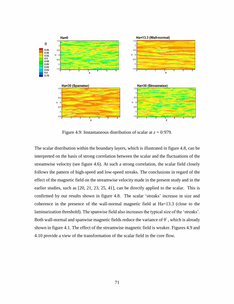
71
Figure 4.9: Instantaneous distribution of scalar at z = 0:979.
The scalar distribution within the boundary layers, which is illustrated in figure 4.8, can be
interpreted on the basis of strong correlation between the scalar and the fluctuations of the
streamwise velocity (see figure 4.6). At such a strong correlation, the scalar field closely
follows the pattern of high-speed and low-speed streaks. The conclusions in regard of the
effect of the magnetic field on the streamwise velocity made in the present study and in the
earlier studies, such as [20, 21, 23, 25, 41], can be directly applied to the scalar. This is
confirmed by our results shown in figure 4.8. The scalar ‘streaks’ increase in size and
coherence in the presence of the wall-normal magnetic field at Ha=13.3 (close to the
laminarization threshold). The spanwise field also increases the typical size of the ‘streaks’.
Both wall-normal and spanwise magnetic fields reduce the variance of θ/ , which is already
shown in figure 4.1. The effect of the streamwise magnetic field is weaker. Figures 4.9 and
4.10 provide a view of the transformation of the scalar field in the core flow.

72
Figure 4.10: Instantaneous distribution of scalar at x = 0.
Figure 4.11: Instantaneous distribution of scalar at y = 0.

73
It has been observed that the transformation is only noticeable in the cases of wall-normal
and spanwise magnetic fields. In both cases, the core flow area shrinks as the boundary
layers become thicker (see figure 4.1). Furthermore, similarly to the velocity components,
the scalar distribution is characterized by larger length scales than in the flow without
magnetic field.
4.3.7 Scalar Structure Anisotropy
The last characteristic of the scalar field explored in the current study is the structure
anisotropy. Similarly to velocity (eqn (3.8) in Chapter-3), the anisotropy is measured by
the coefficient
𝐹𝑖𝑗 ≡⟨(𝜕𝜃/𝜕𝑥𝑖)2⟩
⟨(𝜕𝜃/𝜕𝑥𝑗)2
⟩ , 𝑖 ≠ 𝑗 (4.21)
Fij = 1 corresponds to a perfectly isotropic scalar field, in which the integral length scales
in the directions of are the same. Fij = 0 means a perfectly two-dimensional distribution,
in which does not vary along the coordinate. The results of the computations are shown in
figure 4.11. Anisotropy in the (x-z)-plane (left plot) and (y-z)-plane (right plot) is
presented. Comparing the scalar anisotropy coefficients with the velocity anisotropy
coefficients shown in figure 3.9, strong similarities especially with the anisotropy of the
streamwise velocity are found per figure 4.11.
Figure 4.12: Scalar anisotropy coefficients F13 (left) and F23 (see (4.19)).

74
Near the walls, where θ/ is in almost perfect anti-correlation with u/, strong wall-normal
derivatives results in very small F13 and F23. In the core flow area, the scalar distribution
becomes more isotropic, although the coefficients never reach 1.0, i.e., the integral length
scales in the streamwise and spanwise directions remain larger than the wall-normal scale.
The only significant effect of the magnetic field on the scalar anisotropy is in the case of
the spanwise field (see figure 4.11). The spanwise field is known to increase the typical
spanwise and streamwise length scales of velocity (ref [13] and figure 3.9 in Chapter 3).
The same effect for the velocity and the corresponding decrease of the anisotropy
coefficients for the scalar has been observed in the current study.
4.4 Conclusion
The main results of the presented work concern the effect of the magnetic field on the scalar
distribution and the rate the turbulent scalar transport across the channel. In the range of
the Hartmann numbers considered, the effect is found to be strong in the cases of wall-
normal and spanwise magnetic field, but less so in the case of streamwise field. The
turbulent scalar flux is substantially reduced (see figure 4.4) due to the suppression of wall-
normal velocity fluctuations and some loss of correlation between the scalar and the wall-
normal velocity. This results in reduction of the Nusselt number. As illustrated in figure
4.5, for all three orientations of the magnetic field, the decrease of Nu −1 is rather
accurately approximated by linear functions of the magnetic interaction parameter N.
It is interesting that the transformation of the mean scalar profiles in figure 4.1 is
qualitatively similar to the transformation observed in the hydrodynamic case at decreasing
Pr [49, 52]. Both the transformations are caused by suppression of the wall-normal
turbulent transport of the scalar. The mechanisms of suppression are, however, different.
In the low-Pr flows, high molecular diffusivity acts as a ’filter’ preventing the formation
of scalar fluctuations with short wavelengths, thus removing the short-wavelength
component of the transport. In the MHD case, as it has been demonstrated through current

75
study, the mechanism is that of suppression of the wall-normal velocity fluctuations and
reduction of velocity-scalar correlation by the magnetic field.

76
CHAPTER V
SCALAR TRANSPORT AND PERTURBATION DYNAMICS IN
INTERMITTENT MHD FOW
5.0 Introduction
The influence of magnetic field on turbulent flow and scalar transport characteristics of
electrically conducting fluid have been discussed in Chapter 3 and 4 which highlights main
features of the flow such as, turbulence suppression, development of Hartmann Boundary
Layer and anisotropy, degradation of scalar transport etc. Apart from the features discussed
so far, there exists a unique flow regime in electrically conducting fluid especially liquid
metal for the case of spanwise magnetic field which was first discussed in [15]. Similar
regimes exist in all MHD systems without solid walls crossing the magnetic field line [13,
76]. It is characterized by long periods of nearly steady, two-dimensional (2D) flow
interrupted by violent three-dimensional bursts. Contrary to the over-simplification that the
magnetic field always dumps turbulence and helps to reduce undesired velocity
fluctuations, the regime features novel characteristics of the flow where the flow repeats
itself in violent transitioning between 2D state where turbulence is fully suppressed, and
fully turbulent three-dimensional (3D) states. The new regime which is defined as Large-
scale Intermittency [15] occurs in a wide range of parameters (e.g. Harmann number) and
have implications for metallurgical and other low-Rm technological flow. A case example
is continuous casting of steel described in Chapter 1. During the casting process, the mixing
and transport can be increased primarily when the turbulent burst happens due to
intermittency. However, when the flow transforms to quasi-2D state due to magnetic
damping by the imposed magnetic field, the flow fluctuation and mixing reduced which

77
results in inhomogeneous casting of steel. Similar phenomena may happen in admixtures
transport (e.g. Growth of Crystal described in Chapter [15]).
In the current study, the work in Ref [15] is further comprehended by conducting direct
numerical simulation (DNS) to analyze features of the intermittent regime, such as
transport of a passive scalar, distribution of perturbation energy between mean flow and
fluctuations, and the effect of the strength of the magnetic field which provides sort of
book-end on influence of imposed uniform magnetic field on turbulent and scalar transport
characteristics in a channel. In this chapter, the results of the scalar transport and
perturbation dynamics in intermittent MHD has been discussed. The outcome of the
discussed results in this chapter is published in the research article [54].
5.1 Background and review on earlier work
The large-scale intermittency discovered in [15] occurs in a certain range of the magnetic
field strength, where the flows experience cycles with long periods of nearly laminar,
nearly two-dimensional behavior interrupted by relatively brief turbulent bursts. The key
to understanding the large-scale intermittency is the direct effect of the Joule dissipation of
induced electric currents on the flow. The dissipation rate is proportional to the square of
the velocity derivative in the direction of the magnetic field [1]. The flow structures with
large derivatives are suppressed, while the structures uniform along the magnetic field lines
do not induce electric currents and, therefore, remain unaffected. The situation becomes
more complex in systems with Hartmann walls (walls perpendicular to the magnetic field).
In this case, the global distribution of electric potential causes currents and Joule
dissipation within the Hartmann boundary layers even when the flow structures in the core
are uniform along the magnetic field. In Ref. [15], the large-scale intermittency was
demonstrated for the channel flow with spanwise magnetic field, i.e. for the case when the
Hartmann walls are absent. The driving mechanism of the intermittency is the classical
Tollmien-Schlichting (TS) instability of the laminar channel flow to two-dimensional
spanwise rolls. Since these structures are uniform in the direction of the magnetic field,
they do not experience suppression due to the Joule dissipation. However, when the rolls

78
develop to a finite amplitude and give rise to secondary three-dimensional instabilities and,
then, to turbulence, strong Joule dissipation appears. It suppresses the turbulence and
returns the flow into a state close to the laminar base flow. The process then repeats in
cycles of transitions between two unstable attractors: the laminar base flow and the three-
dimensional turbulence. Interestingly, the two-dimensional non-laminar solution obtained
in the simulations with imposed two-dimensionality [55] or at stronger magnetic fields is
never approached by the intermittent flow. The mechanism just described appears to be of
general kind, not limited to the specific configuration of the channel flow with spanwise
field. It can be hypothesized that the intermittency may develop if two necessary conditions
are satisfied: (1) the flow may experience a hydrodynamic instability, whose development
is not affected or only weakly affected by the magnetic field, and (2) the magnetic field is
not strong enough to prevent development of three-dimensional secondary instabilities, but
strong enough to suppress the resulting turbulence.
The validity of the hypothesis is demonstrated by two other examples, in which similar
intermittent behaviors are observed: the periodic box turbulence with large-scale forcing
[13, 56] and the ideal flow in a tri-axial ellipsoid [57]. In more realistic systems, the first
of the two conditions listed above practically limits the possible configurations to those
with either infinite or large dimension in the direction of the magnetic field. Still, one can
think of numerous situations, including those with large magnetic Reynolds numbers, in
which the intermittency is possible. It should be also noted that the scenario just described
remains valid if the magnetic field is replaced by another physical mechanism that
suppresses three-dimensional perturbations, but allows unimpeded development of a two-
dimensional instability. An example is recently provided by simulations of a channel flow
with rotation around the spanwise axis [58]. The spanwise rotation suppresses turbulence
on one, so-called stable, side of the channel [59, 60]. It does not, however, affect the growth
of purely spanwise TS rolls. The resulting flow dynamics obtained in Ref. [58] at the bulk
Reynolds numbers between 5000 and 30,000 and sufficiently high rotation rates is
remarkably similar to the large-scale intermittency in the MHD channel observed in Ref.

79
[15]. The flow evolves in cycles, each consisting of growth of TS rolls, their three-
dimensional breakdown, and return to the base state. Depending on the magnitude of the
rotation rate, the intermittency occurs only on the stable side of the channel, the other side
remaining turbulent, or in the entire channel. The time of the process is about 1000
convective time units, which is close to the period observed in Ref. [15] for the MHD
channel flow.
From the viewpoint of general hydrodynamics, the large-scale intermittency is a
manifestation of transition between laminar and turbulent states. The situation, in which
the transition leads to localized, either in space or time, turbulent zones (sometimes called
patterned turbulence phenomena [61] is not uncommon. It can be mentioned the turbulent
patches in pipe, channel, boundary layer, and other parallel shear flows [61-65] and the
striped turbulence in Taylor and plane Couette flows [66-69] that typically takes the form
of oblique turbulent stripes and requires large streamwise and spanwise dimensions of the
computational domain to be detected in simulations. The common feature of all these
flows, also present in our case, is the range of parameters, in which a linear or nonlinear
instability mechanism is sufficiently strong to create turbulence, but the turbulence lacks
ability of self-sustaining in the entire flow domain or over a long period of time.
In the current study, the intermittency in the case of the channel flow with spanwise
magnetic field is further studied. Attention is given to the transport properties of the flow,
distribution of the perturbation energy between mean flow and fluctuations, and the effect
of the strength of the magnetic field.
5.2 Model for the intermittency study
A fully developed flow of an incompressible electrically conducting fluid in a plane
channel is considered in the current study similar to configuration described in Chapter 3
and 4 (please refer to figure 2.1 in Chapter 2 for the channel configuration). The walls are
perfectly electrically insulating. The flow is driven by an imposed streamwise pressure
gradient maintained so that the total flow rate is constant. A uniform constant magnetic

80
field of strength B is applied in the spanwise (parallel to the walls and perpendicular to the
mean flow) direction. A passive scalar field θ (e.g., temperature or concentration of an
admixture) is present in the flow. The magnetic Reynolds and Prandtl numbers are assumed
to be much smaller than one, which corresponds to a typical situation in technological or
laboratory flows of liquid metals and other electrically conducting fluids. As a result, the
induced magnetic field is much smaller than the imposed magnetic field and can be
neglected in the Ohm’s law and the Lorentz force. The quasistatic approximation described
in chapter 2 [1] is valid. The equations in non-dimensional form are
𝜕𝒖
𝜕𝑡+ (𝒖. ∇)𝒖 = −∇𝑝 +
1
𝑅𝑒∇𝟐𝒖 + 𝐍(𝐣 × 𝒆𝒚) (5.1)
∇. 𝒖 = 𝟎 (5.2)
𝒋 = −∇𝝋 + 𝒖 × 𝒆𝒚 (5.3)
∇2𝜑 = ∇. (𝒖 × 𝒆𝒚) (5.4)
𝜕𝜃
𝜕𝑡+ 𝒖. ∇𝜃 =
1
𝑃𝑟𝑅𝑒∇2𝜃 (5.5)
where u = (u, v,w), p, θ, j, and φ are velocity, pressure, passive scalar, current density, and
electric potential fields, respectively. The streamwise, spanwise, and wall-normal
coordinates are, correspondingly, x, y, and z. The unit vector ey represents the direction of
the magnetic field.
The boundary conditions in the streamwise and spanwise directions are those of periodic
velocity, pressure perturbations, scalar, and electric potential. The channel walls are subject
to no slip velocity condition, perfectly electrically insulating, and maintained at constant
values of the scalar:

81
𝑢 = 0 𝑎𝑡 𝑧 = ±1 (5.6)
𝜕∅
𝜕𝑛= 0 𝑎𝑡 𝑧 = ±1 (5.7)
𝜃 = 1 𝑎𝑡 𝑧 = −1, 𝜃 = 0 𝑎𝑡 𝑧 = 1 (5.8)
The typical scales used for non-dimensionalization are the channel half-width L as the
length scale, mean velocity U as the velocity scale, L/U as the time scale, ρU2 as the
pressure scale, the strength of the imposed magnetic field B as the magnetic field scale,
ULB as the scale of electric potential, σUB as the scale of current density, and the scalar
difference between the walls as the scale for the scalar field.
The non-dimensional parameters of the model are the Reynolds number (2.17), Prandtl
number (2.18) and either the Hartmann number (2.37) or the magnetic interaction
parameter (2.38).
The equations and boundary conditions have the laminar, steady-state “base flow” solution
with parabolic velocity profile and purely diffusive scalar transport
𝒖𝑏𝑎𝑠𝑒 = (3/2)(1 − 𝑧2)𝑒𝑥, 𝜃𝑏𝑎𝑠𝑒 = (1/2)(1 − 𝑧) (5.9)
It can be noted that, in addition to being an exact solution for the channel flow with
spanwise magnetic field, ubase is an asymptotic limit of the velocity distribution in the core
(outside the Hartmann boundary layers) of the flow in a rectangular duct of large aspect
ratio with the imposed magnetic field parallel to longer sides. This can be obtained from
the expansion series solution [3] of the MHD duct flow or numerically, as in Ref. [70].
According to Ref. [70], in the range of Ha considered in this paper, ubase is a good
approximation of the core flow velocity at aspect ratios above 10.

82
The problem is solved numerically following the DNS approach. The numerical method is
based on the second-order finite difference scheme described as the scheme B in Ref. [74],
the details of which has been discussed in chapter 2. The method has been extended in Ref.
[35] to include the solution of the scalar transport equation (5.5). The scheme utilizes the
explicit backward-difference/Adams-Bashfort scheme for time discretization and the
standard projection technique to satisfy incompressibility. The spatial discretization is on
a spatially non-uniform structured collocated grid. Velocity and current fluxes at half-
integer grid points are obtained by interpolation and applied in evaluation of differential
operators to ensure that the scheme is nearly fully conservative in regard of the mass,
momentum, energy, scalar, and electric charge conservation principles [71, 75]. Further
details can be found in Chapter 2 per Ref. [74] as well as in the recent works, where the
scheme was applied [35, 72, 73].
The simulations are conducted at the Reynolds number of 5333, which is the same as the
Reynolds number used by Ref. [15], where it was presented as 8000 based on the channel
half-width and the centerline velocity of the laminar flow. The value is higher than the
linear stability limit of the hydrodynamic channel flow Re = 3848. The explored range of
the Hartmann number is 30 ≤ Ha ≤ 160.
The Prandtl number Pr = 1 is chosen for all the computations. As a justification, the current
study considers that the values of Prandtl and Schmidt numbers in the technological
applications involving liquid metals vary from those much smaller than one (Prandtl
number in heat transfer) to those much larger than one (Schmidt number in transport of
certain admixtures). Since the current investigation is the first in nature, in which the scalar
transport in the presence of large-scale intermittency is considered, the study considers Pr
= 1 and limit the discussion of the effect of Pr (undoubtedly significant) to the qualitative
arguments given in the conclusion of this chapter.

83
The computational domain has the dimensions of 2π ×4π ×2 in the streamwise, spanwise,
and wall-normal directions, respectively. The computational grid consists of 64 × 64 × 80
points. The points are distributed uniformly in the streamwise and spanwise directions and
clustered toward the walls using the coordinate transformation z = tanh (Aζ )/tanh (A) with
A = 1.5. The grid is similar to the grid used in [15], the differences being that the current
study uses finite difference rather than pseudo-spectral discretization and that the number
of grid points in the wall-normal direction is slightly larger in the current study (Ref. [15]
used 64 Chebyshev functions).
One may argue that the choice of the domain size and numerical resolution in current study
is inadequate, because smaller grid steps are needed to fully resolve the small-scale motions
during the turbulent bursts and because larger streamwise size of the domain is needed to
capture the long-range interaction of the evolving TS rolls. The justification of the current
study approach is two-fold. First, as discussed in Ref. [15], the mechanisms and major
features of the process are not significantly affected by the small-scale resolution and the
domain size. Second, the intermittency has a very large time scale, which requires
simulations of flow evolution during tens of thousands of time units. Performing such
simulations with a significantly finer grid and in a substantially larger domain would be
either computationally unfeasible or feasible in the form of very large-scale massively
parallel computations. It is considered unnecessary in the current study and a somewhat
inaccurate numerical model is used as a compromise.
5.3 Results and Discussion
One simulation of a flow realization is conducted for every explored value of Ha. In each
run, the computation started with the developed turbulent flow at Ha = 30 and conducted
the computations until a pattern of regular cyclic transitions between laminar and turbulent
states has been established. After that, the simulation is continued for not less than ten
cycles. Flow properties are studied, and time-averaged statistics is accumulated during this
period.

84
5.3.1 Flow evolution and perturbation energy
The current study differs from the procedures followed in Ref. [15] in the numerical
method on how flow evolves in intermittency cycle. In the spectral method solution of Ref.
[15], random noise of average amplitude 10−6 was constantly added to the velocity field
thus setting the “floor” of the perturbation energy during the periods of nearly laminar
behavior. Noise is not added in the current simulations. It is found that in the finite
difference solution, presumably due to the discretization error, the floor has been
repeatedly reproduced at some small energy (see figure 5.1). For the purpose of
verification, the run at Ha =100 is repeated with the noise added. No significant differences
in the results in comparison with the no-noise run has been detected.
The current numerical model has been verified comparing the results obtained at Ha = 80
with those published in [15]. Good agreement is found for the integral characteristics of
the process, such as the peak magnitude of the perturbation energy. The lengths of the
intermittency cycle are only slightly different. This shows that the addition of weak random
noise and the numerical dissipation of the finite difference discretization do not
significantly affect the intermittent behavior.

85
Figure 5.1: Evolution of the kinetic (a, c, e) and scalar (b, d, f) energies of the
perturbations during two cycles of large-scale intermittency at Ha = 80.

86
The large-scale intermittency has been detected in the current study simulations at 40 ≤ Ha
≤ 140. At smaller Hartmann numbers, as found from the computations at Ha =30, the flow
remained persistently turbulent, although the nature of the turbulence was significantly
modified by the spanwise magnetic field in the manner described in earlier publications
[35, 25]. At higher Ha, the flow becomes purely 2D channel flow [55]. This is found in
the current study simulations with Ha = 160. For all the intermittent flow regimes, perfectly
periodic behavior of the integral characteristics of the flow has been demonstrated from the
simulation. In particular, the length of a cycle has been virtually constant, and the peak
amplitudes of velocity and scalar perturbations has demonstrated only slight variations.
Further in this section, the flow behavior during an intermittency cycle has been analyzed.
The analysis is different from Ref. [15] in three aspects. One is that the present study
investigates the transport properties of the flow by analyzing the behavior of a passive
scalar field. Another is that in the current study the modification of the mean flow during
the cycle has been considered. The current study also presents the data illustrating how the
characteristics change with the Hartmann number. The flow evolution is described in terms
of growth and decay of velocity and scalar perturbations. The perturbations are defined
with respect to the base flow (5.9):
𝒖′ = 𝒖 − 𝒖𝒃𝒂𝒔𝒆, 𝜃′ = 𝜃 − 𝜃𝑏𝑎𝑠𝑒 (5.10)
and, as in Ref. [15], with respect to the instantaneous mean flow:
𝒖′′ = 𝒖 − ⟨𝒖⟩, 𝜃′′ = 𝜃 − ⟨𝜃⟩ (5.11)
where ⟨ ⟩ is averaging in the x − y plane, and the scalar perturbations θ” analogous to the
velocity perturbations u” computed in Ref. [15] has been introduced in the simulation. The
need for the two types of perturbations stems from the intention to consider the evolution
of their difference, which is, evidently, the distortion of the mean velocity and scalar:

87
∆𝒖 ≡ 𝒖′ − 𝒖′′ = ⟨𝒖⟩ − 𝒖𝒃𝒂𝒔𝒆, ∆𝜃 ≡ 𝜃′ − 𝜃′′ = ⟨𝜃⟩ − 𝜃𝑏𝑎𝑠𝑒 (5.12)
The distortion develops during the stages of the flow evolution when the perturbation
amplitude is finite. As will be seen in the following, it plays a significant role in the energy
balance during an intermittency cycle. In order to quantify the evolution of the flow, kinetic
and scalar energies as volume averages of, respectively, square of velocity and scalar have
been computed. For example, the total energies are
𝐸 = 𝑉−1 ∫ 𝒖2𝑑𝑉𝑉
, 𝐸𝜃 = 𝑉−1 ∫ 𝜃2𝑑𝑉𝑉
(5.13)
In a similar way, the energies 𝐸′, 𝐸𝜃′ of the perturbations (5.10), energies 𝐸", 𝐸𝜃
" of the
perturbations (5.11), and the energies ∆𝐸, ∆𝐸𝜃 of the distortion of mean velocity and scalar
(5.12) have been computed.
It is straightforward to derive the following relations between the energies just introduced:
𝐸′ = 𝐸" + ∆𝐸, 𝐸𝜃′ = 𝐸𝜃
" + ∆𝐸𝜃, (5.14)
𝐸 = 𝐸𝑏𝑎𝑠𝑒 + 𝐸′ + 𝐸𝑚, 𝐸𝜃 = 𝐸𝜃𝑏𝑎𝑠𝑒 + 𝐸𝜃′ + Eθm (5.15)
In the last formula, Ebase and Eθbase are the energies of the base flow and scalar distribution
(5.9) and
𝐸𝑚 = 2𝑉−1 ∫ (𝒖𝑏𝑎𝑠𝑒 . ∆𝒖)𝑑𝑉𝑉
, 𝐸𝛩𝑚 = 2𝑉−1 ∫ (𝜃𝑏𝑎𝑠𝑒∆𝜃)𝑑𝑉𝑉
(5.16)
are the terms that appear as a result of our decomposition of the mean fields into the base
and distortion components. Further understanding of the flow behavior is provided by
considering separately the evolution of the velocity and scalar components uniform in the
spanwise (y) direction usp, θsp and the components uniform in the streamwise (x) direction

88
ustr , θstr. The components are found by averaging the computed fields in the respective
directions. Their energies will be referred to as 𝐸𝑠𝑝′ , 𝐸𝜃𝑠𝑝
′ , 𝐸𝑠𝑡𝑟′ , 𝐸𝜃𝑠𝑡𝑟
′ if computed for
perturbations (5.10) and as 𝐸𝑠𝑝" , 𝐸𝜃𝑠𝑝
" , 𝐸𝑠𝑡𝑟" , 𝐸𝜃𝑠𝑡𝑟
" if computed for perturbations (5.11).
At last, with the purpose of separating the secondary instabilities leading to a turbulent
burst from the growth of TS rolls and the mean flow distortion, the energies E3D, Eθ3D of
the components of the perturbations (5.10) non-uniform in the spanwise direction and
defined as 𝒖𝟑𝑫′ = 𝒖′ − 𝒖𝒔𝒑
′ , 𝜃3𝐷′ = 𝜃′ − 𝜃𝑠𝑝
′
5.3.2 Velocity during an intermittency cycle
The typical intermittent behavior is illustrated in Fig. 5.1 that presents the results obtained
at Ha = 80. Only two of the ten cycles computed during the stage of a fully developed flow
are shown. Figure 5.1(a) shows the kinetic energy of the velocity perturbations (5.15)
defined, as in Ref. [15], with respect to the instantaneous mean flow. As it can be observed
that a cycle can be divided into three stages indicated in Fig. 5.1 by the typical time
moments t1, t2, t3. The velocity perturbations u” during each of these moments are illustrated
in Fig. 5.2. During the first stage, to which can be referred to as the “growth stage”, the
velocity field is nearly perfectly spanwise-independent (𝐸′ ≈ 𝐸𝑠𝑝" as can be seen in Fig.
5.1(a)). Its energy grows due to the amplification of unstable Tollmien-Schlichting (TS)
rolls (see Fig. 5.2(a)), which are uniform in the spanwise direction and, thus, not affected
by the magnetic field.

89
Figure 5.2: Evolution of perturbation velocity u” and scalar θ” during one cycle at Ha = 80.
(a) Velocity vectors and scalar distribution in a cross-section y = const at t = t1 during the
growth stage (see Fig. 5.1) when velocity and scalar perturbations are nearly purely
spanwise-independent. (b) and (c): Isosurfaces of u” and θ” at t = t2 during the turbulent
burst. For u”, the range is [−0.47, 0.35], the isosurfaces at u” = − 0.15, and 0.15 are shown.
For θ”, the range is [−0.25, 0.26], the isosurfaces at θ” =−0.09, and 0.09 are shown. (d) and
(e): Isosurfaces of u” and θ” at t = t3 during the decay stage. For u”, the range is [−0.023,
0.038], the isosurfaces at u” =−0.01, and 0.01 are shown. For θ”, the range is [−0.059,
0.059], the isosurfaces at θ” =−0.02, and 0.02 are shown.
The second stage, which can be called a “burst,” starts when the TS rolls experience
secondary instability leading to turbulence (see Fig. 5.2(b)). This transfers the energy into
3D velocity fluctuations. As demonstrated in [15], this causes Joule dissipation, which is

90
sufficiently strong to suppress the turbulence and initiate the third stage, namely the stage
of “decay.” As demonstrated in [15], the decay of 3D kinetic energy is primarily due to the
direct suppression by the Joule dissipation, while the decay of 𝐸𝑠𝑝" is, apparently, due to the
viscous dissipation and transfer of energy into 3D perturbations. As can be seen in Fig.
5.1(a), the perturbation energy at this stage is almost entirely in streamwise-independent
velocity. It is illustrated in Fig. 5.2(d) and discussed in Ref. [15] that, at this stage, the
perturbations u” are dominated by streamwise streaks.
Figure 5.1(c) shows the terms of the decomposition (5.14) of the perturbation kinetic
energy. It can be observed that, during the growth stage, the perturbations u’ measured with
respect to the base state are nearly identical to the perturbations u” with respect to the
instantaneous mean flow. The mean flow distortion has the energy 𝛥𝐸 several orders of
magnitude smaller than 𝐸′ ≈ 𝐸". 𝛥𝐸 starts to grow rapidly when the TS rolls reach high
amplitude and becomes of the same order of magnitude as 𝐸′ and 𝐸" during the turbulent
burst. After the burst, 𝐸"decreases much faster than 𝐸′ and 𝛥𝐸 and soon becomes negligibly
small. During the decay stage, 𝐸′ ≈ 𝛥𝐸, i.e., the perturbations are almost entirely in the
form of the distortion of mean flow. The streamwise streaks identified in [15] and
illustrated in Fig. 5.2(d) dominate the velocity deviation from the instantaneous mean, but
are, in fact, negligible in comparison with the simultaneous distortion of the mean velocity
profile. The persistence of the mean flow distortion during the decay phase is easy to
explain. Being spanwise-uniform, this component is not affected by the Joule dissipation,
while its large typical length scale results in weak viscous dissipation.

91
Figure 5.3: Profiles of mean velocity ⟨𝑢⟩ and scalar ⟨𝜃⟩ and their deviations 𝛥𝑢, 𝛥𝜃 from
the base flow (5.9). The profiles are shown at Ha = 80 for the typical time moments during
the stages of 2D growth (t1), turbulent burst (t2), and decay (t3) (see Fig. 5.1). The scalar
profiles are also shown for the time moment t4 typifying the stage of “sub-diffusive” scalar
transport (see Fig. 5.6).
The profiles of instantaneous mean velocity ⟨𝑢⟩(z, t) and its distortion 𝛥𝑢 at the typical
time moments t1, t2, and t3 are shown in Fig. 5.3. Significant distortion has been observed
during the turbulent burst at t = t2 and almost as strong in the decay phase at t = t3.

92
The global balance of kinetic energy has been obtained through the computations per
(5.15). A peculiar feature of the balance is the behavior of the total kinetic energy E with
respect to the base flow level Ebase = 1.2. During the growth stage, increase of the
perturbation energy E’ leads to increase of E well above Ebase. The relation changes during
the turbulent stage. The total energy E drops rapidly and becomes noticeably smaller than
Ebase. It remains smaller well into the decay stage. This seemingly paradoxical behavior is
related to the large negative value of Em in (5.15) (see Fig. 1(e)). An explanation can be
seen in Figs. 5.3(a) and 5.3(c). The mean flow distortion ⟨𝑢⟩, while conserving the total
flow rate, reduces ⟨𝑢⟩ in the high-speed core, thus transforming the profile into one with
lower energy.
The profiles of the x − y-averaged rms perturbations of the velocity components are shown
in Figs. 4(a)–4(c). The perturbations are computed as in (5.14), i.e., with respect to the base
flow. The profiles at t = t1 show the effect of the TS rolls, which generate u’ and w’, but not
v’. The profiles at t = t2, when the flow is apparently turbulent, show significant differences
with the profiles observed in the fully developed turbulent flows in a channel with a
spanwise magnetic field [25]. In particular, the peaks of ((𝑢′2)1/2) are much farther from
the wall in our case than in a developed turbulent flow. For ((𝑤′2)1/2), a distribution with
the maximum in the middle instead of the distribution with two maxima not far from the
wall typical for developed turbulence is observed. During the decay stage, at t = t3, the
perturbations are predominantly in the streamwise velocity component, which is in full
agreement with the fact that the perturbations at this stage consist of the mean flow
distortion and streak-dominated perturbations u” (see Figs. 5.1 and 5.2(d)).

93
Figure 5.4: Profiles of x-y-averaged rms perturbations of velocity components and scalar
at Ha = 80 at the stages of 2D growth (time t1), turbulent burst (t2), and decay (t3) (see
Fig. 5.1).
The wall-normal momentum transport by the velocity fluctuations is illustrated in Fig.
5.5(a) by the profiles of the Reynolds stress component 𝜏13 ≡ ⟨𝑢′𝑤′⟩. The transport is only
noticeably strong during the turbulent burst. The computations of the correlation
coefficient 𝜏13/((𝑢′2)1/2(𝑤′2)1/2) have shown that, in addition to much larger amplitude
of fluctuations, this is caused by stronger correlation between u’ and w’.
The discussion of the evolution of velocity field during an intermittency cycle is concluded
by the data in Fig. 5.6(a) presenting the skin friction coefficient Cf. In non-dimensional
units, Cf is defined as the imposed pressure gradient needed to drive the flow. In agreement

94
with [15], Cf grows nearly twice the base flow level during the turbulent burst, when strong
wall-normal momentum transfer is generated by velocity fluctuations, but remains very
close to the base flow level during the rest of the cycle.
Figure 5.5: Profiles of x-y-averaged wall normal transport rates of momentum and scalar
at Ha = 80 at the stages of 2D growth (time t1), turbulent burst (t2), and decay (t3)
(see Fig. 5.1).
Figure 5.6: Evolution of the skin friction coefficient (a) and Nusselt number (b) at Ha = 80
during the same two cycles as in Fig. 1. Two horizontal lines show the values for the base
flow state (5.13) and the perfectly 2D flow [55] obtained in our case at Ha = 160 and higher.

95
5.3.3 Passive scalar during an intermittency cycle
The evolution of the scalar field during an intermittency cycle at Ha = 80 is presented in
Figs. 5.1–5.6. Various characteristics are shown in parallel with the respective
characteristics of velocity. Considering the energy curves of the scalar perturbations θ”
with respect to the instantaneous mean distribution (see Fig. 5.1(b)) and the spatial structure
of θ” at the typical time moments (see Figs. 5.2(a), 5.2(c), and 5.2(e)), It can concluded that
the scalar field goes through the same three stages as the velocity field.
In the growth stage, the scalar energy 𝐸𝜃" is practically identical to the energy of the
spanwise uniform instability modes 𝐸𝜃𝑠𝑝" . A prominent feature of the scalar distribution at
this stage is the sheet-like zones of large positive and negative θ” extending along the walls
(see Fig. 5.2(a)). The absence of strong correlation between u” and θ” visible in Fig. 5.2(a)
is because of the difference between the speeds of streamwise transport of the scalar (the
local speed of the mean flow) and the phase speed of the moving TS rolls.
During the turbulent burst, the quasi-2D structure of the scalar perturbations breaks down
into a three-dimensional distribution that has the typical spanwise length scale similar to
the scale of velocity distribution (see Fig. 5.2(c)). In the decay stage, the scalar
perturbations are nearly streamwise independent (𝐸𝜃" ≈ 𝐸𝜃𝑠𝑝
" in Fig. 5.1(b)) and are
dominated by streak-like structures (see Fig. 5.2(e)).
Considering the decomposition of the scalar perturbations θ’ into the deformation of the
mean scalar profile 𝛥𝜃 and the perturbations with respect to the instantaneous mean θ”
(see Fig. 5.1(d)), it is found that, similarly to velocity, 𝛥𝜃 is negligibly weak during the
growth stage, but is much stronger than θ” during the decay stage, when it constitutes
practically entire θ’. Similarity to velocity field in the behavior of the total energy of the
scalar 𝐸𝜃 (see Fig. 5.1(f)) is also seen. It increases above the base flow level 𝐸𝜃𝑏𝑎𝑠𝑒 = 1/3
during the late growth and early turbulent stages. After the peak of the turbulent burst, 𝐸𝜃

96
drops sharply below 𝐸𝜃𝑏𝑎𝑠𝑒 as a result of the mean flow transformation causing negative
𝐸𝜃𝑚 in (5.15).
The qualitative similarity between the evolutions of scalar and velocity is not surprising,
since the second largely determines the first. At the same time, certain differences are
observed. One is that the energy of scalar perturbations decays much slower after the burst
than the kinetic energy. This is true for the perturbations with respect to instantaneous mean
(cf. Figs. 5.1(a) and 5.1(b)) and with respect to the base state (cf. Figs. 5.1(c) and 5.1(d)).
As a result, the minimum levels reached by the scalar perturbation energies are several
orders of magnitude higher than the minima of kinetic energies. The slower decay of the
scalar can be explained by the fact that the scalar is not directly affected by the Joule
dissipation. Its decay is caused solely by diffusion.
Yet another difference between the dynamics of the scalar and velocity fields can be
observed in Fig. 5.1. The visible switch from decay to growth occurs significantly
(hundreds of time units) later for the scalar than for velocity. This cannot be attributed to
the delayed correlation buildup between velocity and scalar, since the time needed for the
buildup is ∼1 in our variables. The correct explanation is that the “switch” indicates the
time moment when the energy associated with the growing TS rolls exceeds the energy of
the decaying components. Since the decay is slower for the scalar than for velocity, the
“switch” occurs at a higher amplitude of growing perturbations and, thus, at a later time.
The transformation of the mean scalar ⟨𝜃⟩(z, t) and its deviation 𝛥𝜃 from the base flow
distribution (5.13) is illustrated in Figs. 5.3(b) and 5.3(d). It is evident that strong
transformation develops during the turbulent burst and persists during the decay stage (see
profiles at t = t2 and t = t3). The transformation is rather peculiar in its dissimilarity to the
transformation observed in the fully developed turbulent flows (see, e.g., Ref. 35).
Boundary layers similar to those in a turbulent flow develop near the walls. The shape of
the profile between the boundary layers is, however, quite different from the nearly straight
line typical for turbulent flows. As the middle of the channel is considered, the slope

97
becomes nearly zero just outside the boundary layer and then increases rising above the
slope of a laminar profile.
The rms scalar perturbations (𝜃′2)1/2 and the wall-normal scalar transport by velocity
fluctuations 𝑞𝑡 = ⟨𝑤′𝜃′⟩ are shown, respectively, in Figs. 5.4(d) and 5.5(b) illustrate two
interesting features of the scalar evolution. One is that the spatial distribution of (𝜃′2)1/2
tends to be more similar to the distribution of (𝑢′2)1/2 than (𝑤′2)1/2. The correlation
coefficients 𝑅𝑢𝜃 = ⟨𝑢′𝜃′⟩/((𝑢′2)1/2(𝜃′2)1/2 has been computed (not shown) and found
that Ruθ is consistently larger than Rwθ . This dominance of the streamwise velocity
component in determining the passive scalar distribution is known from the studies of
turbulent scalar transport in shear flows. The main explanation is that u/ is simply stronger
than w/.
Another interesting feature is the distribution of scalar flux qt during the turbulent burst
(t = t2 in Fig. 5.5(b)). qt has two “bulges” near the walls, but is small in the middle of the
channel. It has been found that the suppression of the scalar transport is primarily due to
almost zero correlation between w’ and θ’ in the middle. The “bulges” of qt provide an
explanation of the peculiar shape of ⟨𝜃⟩ at t2 and t3 observed in Fig. 5.3. Applying, as an
approximation, the steady-state balance of the x − y-averaged wall-normal scalar transport
(see, e.g., Ref. 35 or other works on turbulent scalar transport in channels), it is found that
local increase of qt must be accompanied by corresponding decrease of diffusive transport
and, thus, of the slope of ⟨𝜃⟩.
The transformation of the scalar distribution affects the global wall-to-wall scalar transport,
which we define as the Nusselt number:
𝑁𝑢 ≡ 2𝑑𝑇
𝑑𝑧|
𝑤𝑎𝑙𝑙 (5.17)

98
The wall-normal derivative in (5.17) can be taken at z = −1 or z = 1. The choice may have
a slight effect on the instantaneous values, but the shapes of the curves Nu(t) and the values
obtained by time integration over the intermittency cycle are, of course, the same.
The Nusselt number computed at Ha = 80 is shown as a function of time in Fig. 5.6(b).
Strong (nearly three-fold) increase during the turbulent burst is observed. During the rest
of the cycle, Nu is much smaller, close to the value Nu = 1 of the base flow. Interestingly,
during the significant time period of the late decay and early growth stages, when the flow
is close to its base state, Nu is smaller than 1. The scalar transport can be called “sub-
diffusive.” The effect is found in the present computations in the intermittent regimes at
Ha = 60, 80, 100, 120, and 140. It becomes stronger at higher Ha. The minimum value of
Nu is 0.883 at Ha = 120 and 0.718 at Ha = 140. The phenomenon has been investigated
and it is found that it is caused by a modification of the mean scalar profile. An illustration
is provided in Figs. 5.3(b) and 5.3(d), which shows ⟨𝜃⟩ and 𝛥𝜃 at the moment t4
corresponding, as shown in Fig. 5.6(b), to Nu < 1. The profile deviates from the base state
(5.9) so that the slope |dθ/dz| at the wall is slightly smaller than the base state value 1/2.
The reasons for formation of such a profile become clear if the distribution of the mean
scalar forming in the result of a turbulent burst (see, e.g., curves of ⟨𝜃⟩ and 𝛥𝜃 for t = t3 in
Figs. 5.3(b) and 5.3(d)) is considered. As a result of non-uniform turbulent scalar flux qt
(see Fig. 5.5(b)), the distribution of 𝛥𝜃 has two stronger peaks in the middle of the channel
and two weaker peaks near the walls. The transformation of the profile after the burst is
predominantly controlled by diffusion. It is virtually evident, but has also been confirmed
by the current solution of the one-dimensional diffusion equation, that this transformation
leads to the profiles of ⟨𝜃⟩ and 𝛥𝜃 illustrated by the curves at t = t4 in Figs. 5.3(b) and
5.3(d).
The analogous “sub-viscous” wall-normal momentum transport with Cf below the base
flow value 3Re −1 = 0.00056253 during the late decay and early growth stages is also
detected in the present simulation, but the effect is much weaker and only observed at Ha

99
= 120 and 140. The minimum value of Cf is 0.0005619 at Ha = 120 and 0.000539 at Ha =
140.
5.3.4. Effect of Hartmann number
This section reports the results of our study of the influence of the magnetic field strength,
as defined by the Hartmann number, on the intermittency. At each Ha, integral
characteristics, such as the cycle duration and the maximum and cycle-averaged energies,
are obtained by time-averaging over ten consecutive intermittency cycles. As it has been
already mentioned, variations among the cycles are small, so the data can be considered as
characteristics of an individual cycle. The data for the fully turbulent flow at Ha = 30 and
for the purely 2D (spanwise-uniform) flow at Ha = 160 are included for comparison, where
appropriate.
Considering the nature of the direct (via the Joule dissipation) effect of the magnetic field
on the flow, conjectures can be made concerning the influence of field strength on the
intermittency cycle. As illustrated later in this section, the real behavior is largely in
accordance with the reasoning, although more subtle in some aspects.
The strength of the magnetic field does not affect the growth of the TS rolls, which are
spanwise uniform. On the contrary, the turbulent burst is sensitive to the field strength. A
stronger magnetic field should slow down the development of secondary instabilities, thus
extending the 2D growth phase and allowing the TS rolls to grow longer and to a higher
amplitude before they break down. A stronger magnetic field should also result in stronger
suppression of 3D velocity perturbations and, thus, lower amplitude and smaller duration
of the burst. During the decay phase, a stronger magnetic field should lead to faster decay
of perturbations u” with respect to the instantaneous mean, but cannot directly affect the
mean flow distortion 𝛥𝑢 . The effect of the magnetic field on the scalar is, of course,
indirect, via the velocity field. Taking into account the correlation between the velocity and

100
scalar intermittency cycles demonstrated earlier in this section, similar changes in the
evolution of scalar field are expected.
The time characteristics of the intermittency cycle are presented in Fig. 5.7. The curves of
the kinetic perturbation energy E’ (see Fig. 5.1(c)) are used to evaluate the growth and
decay times measured, respectively, as the intervals, during which E/ grows from a
minimum to a maximum at the peak of a turbulent burst and from a maximum to the next
minimum. As it is predicted, the decay time decreases strongly with Ha. The projected
increase of the growth time, however, does not occur. The tendency is that the growth time
decreases with Ha, albeit significantly slower than the decay time and with some growth
between Ha = 60 and 80 and between Ha = 100 and 120.
To explain this behavior, it can be recalled that the perturbation energy E/ consists of the
energy E” of the perturbations u” with respect to the instantaneous mean and the energy 𝛥𝐸
of the mean flow distortion. During the decay stage, 𝛥𝐸 dominates and the time moment
tmin of minimum E’ is, in fact, the moment when the energy E’ of the growing TS rolls first
exceeds the decaying 𝛥𝐸 (see Fig. 5.1(c)). Stronger suppression of turbulent burst
fluctuations by a stronger magnetic field inhibits the energy transfer from the mean flow
to fluctuations and, as it is found, leads to slower decay of 𝛥𝐸. As a result, the cross-over
moment tmin occurs at higher values of 𝛥𝐸 and E”. The effect is not very strong, but
sufficient to somewhat lengthen the decay stage and, correspondingly, shorten the growth
stage.

101
Figure 5.7: Growth time, decay time (see text for definitions), and total intermittency cycle
time as functions of Ha. The results are obtained by averaging over ten consecutive cycles
of fully developed intermittent flows.
The cumulative effect is that the total cycle length is reduced significantly at higher Ha.
The data illustrating the effect of the Hartmann number on the energy characteristics are
presented in Fig. 5.8. It is shown that the kinetic and scalar energies of the perturbations u/
and θ/ with respect to the base flow (see (5.9)) split into the spanwise-uniform (2D) and
non-uniform (3D) components. The energy curves marked as 2D thus show the
characteristics of 2D TS rolls and mean flow distortion, while the curves marked as 3D
show the energies of 3D fluctuations resulting from the secondary instabilities of the TS
rolls. For the kinetic (Figs. 5.8(a) and 5.8(b)) and scalar (Figs. 5.8(c) and 5.8(d)) energies,
the maximum and average values during a cycle are shown, both obtained by averaging
over ten consecutive cycles of a fully developed flow.
It can be observed that a stronger magnetic field means reduction of the maximum and
average values of the kinetic energy of 3D modes. This is an effect of stronger Joule
suppression of turbulence during the burst. At the same time, the maximum value of the
2D energy has the tendency to increase. Similar tendencies are observed for the energy of
the scalar.

102
Figure 5.8: Maximum and cycle-averaged kinetic and scalar energies of the perturbations
u/ and θ/ with respect to the base flow (5.9). The energies of perturbations uniform (2D)
and non-uniform (3D) in the spanwise direction are shown separately as functions of Ha.
The data are obtained as in Fig. 5.7. The 2D energy points at Ha = 160 correspond to the
purely 2D non-intermittent flow regime obtained at this Ha.
The behavior of the cycle-averaged energies shown in Figs. 5.8(b) and 5.8(d) is a
cumulative result of the change of the time and energy characteristics of the cycle. One can
identify the main tendencies: a stronger magnetic field leading to increase of the energy of
2D spanwise-independent components of velocity and scalar fields (except at small Ha)
and decrease of the energy of 3D components. The just concluded discussion of the effect
of magnetic field strength on the dynamics of an intermittency cycle helps to understand

103
the behavior of the maximum and cycle-averaged friction coefficient and Nusselt number
shown in Fig. 5.9.
Figure 5.9: Friction coefficient Cf and Nusselt number Nu as functions of Ha. Maximum
and cycle-averaged values obtained as in Figs.7 and 8 are shown. The points at Ha = 160
correspond to the purely 2D non-intermittent flow regime. The points at Ha = 30 are for
the sustained turbulent flow obtained at this Ha.
One can think of three limiting values of Cf and Nu: the lowest values corresponding to
the base flow, the significantly higher values corresponding to the fully developed 2D flow,
in which the momentum and scalar transport are provided by finite-amplitude deformed
TS rolls (see Fig. 5.6 and the points at Ha = 160 in Fig. 5.9), and the even higher values of
a turbulent flow. An intermittency cycle is a solution trajectory between the unstable
attractors of the base flow and turbulence. The time spent by the solution near the
turbulence attractor is much smaller than the time spent near the base flow state.
Accordingly, Cf and Nu of intermittent regimes show the cycle-averaged values only
slightly higher than the base flow limits. The effect of the strength of the magnetic field on
the average values is very weak. The maximum values of Cf and Nu are significantly
higher than the base flow and 2D flow limits, but, except at Ha = 40, lower than the values
obtained in a truly turbulent flow at Ha = 30. The effect of Ha on the maximum values of

104
Cf and Nu is to reduce them, which can be attributed to suppression of 3D turbulent
fluctuations by the magnetic field.
5.4 Conclusion
A detailed parametric study of the phenomenon of large-scale intermittency in the MHD
channel flow with spanwise magnetic field has been presented in this section. The current
study expands the understanding on intermittency with complete picture on perturbation
dynamics and energy spectrum during intermittency phenomena. In particular, the
proposed doctoral study on intermittency describes the dynamics of a passive scalar field
and quantify the effect of the intermittency on the transport rate. It is found that the scalar
perturbations and the Nusselt number follow the cyclic evolution correlated with the cycles
of velocity, albeit with some differences and unexpected effects, such as the sub-diffusive
scalar transport during a significant segment of the cycle. Strong deformations of mean
velocity and scalar that dominate velocity and scalar perturbations during the decay stage
have been observed. The effect of the strength of the magnetic field on an intermittent flow
is found to be complex, although the main features can be identified as the stabilization of
the growing TS rolls and suppression of their secondary instabilities and the resulting
turbulence.
A few comments are in order concerning the effect of the parameters of the numerical
model on the results. The spanwise and streamwise sizes of the computational domain are
particularly important in the current study. The streamwise size affects the growth rate and
secondary instabilities of the TS rolls [74, 75]. Increasing this size in the current model
could lead to some change in the duration of the growth phase and the strength of turbulent
bursts, but is not expected to have a substantial effect on the nature of the cycling.
Increasing the spanwise size of the computational domain would activate modes of larger
spanwise wavelengths, which are less susceptible to the suppression by the magnetic field.
The test studies reported in [15] indicate that the result would be the shift of the upper
boundary of the range of Ha, in which the intermittency is observed, to higher values. At

105
the same time, the principal mechanisms of growth and decay causing the intermittency
would not change, so the cycling would remain largely the same. Furthermore, it should be
considered that in any real system the spanwise size is limited by the Hartmann walls. It
would be interesting to conduct the simulations at the same time scale as in the present
study, but in a much larger computational domain. This could, among other possible
results, clarify the relation between the time intermittency and the spatial intermittency in
the form of turbulent stripes observed, among other systems, in the channel flow with
imposed magnetic field [76]. The study has to be left for the future, when it becomes
computationally more feasible. Yet another feature of the numerical model with possible
implications for the intermittency effect, namely the constant flux formulation used in the
present model. To verify the effect, a test run with constant imposed pressure gradient is
conducted, which has been taken equal to the gradient in the laminar base flow at the same
Re. Intermittency cycling with period about 4000 convective time units has been found.
During the bursts, the perturbation energy grows to amplitudes comparable to the
amplitudes reported earlier in this section. The increase of flow resistance during each burst
cause approximately 5% drop of mean flow velocity. This implies reduction of the effective
Reynolds number that assists the magnetic field in suppression of perturbations. After the
suppression, the mean velocity increases back to nearly the base flow value and the next
cycle begins. In order to evaluate the practical implications of the intermittency for the
scalar transport and dispersion, the effect of the Prandtl (Schmidt) number has to be
considered. In liquid metals, the Prandtl number is typically small (∼10−2–10−1). This
means that the heat transfer is dominated by conduction and, probably, affected only
slightly by the turbulent bursts. On the contrary, the Schmidt number tends to be larger
than one. The effect of the intermittency on the admixture transport and dispersion is,
therefore, significant, probably stronger than present study. The possibility of the existence
of a flow cannot be excluded, in which periodic turbulent velocity bursts lead to sustained
turbulent fluctuations of a scalar. This can be a subject of future investigations.

106
CHAPTER VI
1D MODEL FOR FLOW FIELD AND PASSIVE SCALAR TRANSPORT
6.1 Introduction
One of the desired outcomes of a direct numerical simulation (DNS) is the detection of
possible simple relationships between the mean flow characteristics and the problem
parameters. Especially sought for are such relationships for the coefficients of eddy
viscosity and diffusivity, since they may provide a basis for development of simple low-
dimensional models of the mean flow. For example, in present study, a highly desired
outcome would be a set of simple approximate formulas modeling the behavior of eddy
viscosity (νt (z)), eddy diffusivity (αt (z)) and turbulent Prandtl number (Prt (z)). Such simple
formulas derived from DNS are not unheard of in MHD. For example, the LES
Smagorinski constant in homogeneous turbulence was shown in [77] to be well
approximated by a linear function of the anisotropy coefficient (equation 3.8 in Chapter 3).
Accurate empirical relations that would express the effect of magnetic field via parameters
of the problem, such as the Hartmann number Ha, magnetic interaction parameter N, or the
anisotropy coefficients (equation 3.8 in Chapter 3) and (equation 4.21 in chapter 4) are
difficult to formulate. As illustrated in figures 3.5, 4.7, and 4.8, the profiles of eddy
viscosity, diffusivity, and Prandtl number change with the strength and orientation of the
magnetic field in a complex way that does not allow a universal desired interpretation.
However, models can be developed for each specific orientation of the magnetic field. In
this section, this is done for the case of wall-normal magnetic field.

107
6.2 Background
In connection to the approach used in the current study to propose 1D models of mean flow
and scalar for the case of a one-component fully developed flow of an electrically
conducting fluid in a channel with imposed magnetic field, a review is conducted on the
earlier work pertaining to mean flow and turbulence closure models. The review also
provides a background of prior works done in the area where turbulence closure and
transport models are proposed in general framework of DNS apart from the mean flow.
Special attention is given on the eddy diffusivity and eddy viscosity modeling approach in
describing the mean flow characteristics.
Due to the low computational cost, Reynolds-averaged Navier-Stokes (RANS) simulations
are widely used for industrial flow simulations. However, RANS method has limitation in
modeling complex turbulence interactions for the mean flow variables. There exists a
scarcity of available literature on the application of RANS models for MHD flows. In
general, RANS method is applied for MHD flow computations using RANS equations with
standard turbulence models and wall functions. The current effort in regard to RANS
simulation includes improvement on the standard approach through the development of
MHD-specific turbulence models [78, 79] and wall functions.
An electromagnetically extended Reynolds stress transport model is developed by Widlund
et al. [79] by transporting an additional scalar parameter which contained information on
the dimensionality and anisotropy of the turbulence that is induced specifically by
electromagnetic effects. Application of the model to a case of decaying turbulence in the
presence of a magnetic field showed good agreement with DNS data.
Kenjeres er al [78] developed a model of magnetohydrodynamic (MHD) interactions
within the framework of the second-moment closure based on direct numerical simulation
(DNS). The MHD effects are taken care in the transport equations for the turbulent stress
tensor and energy dissipation rate. The validation of the model is conducted in plane

108
channel flows with different orientation of magnetic field against the available DNS (Re =
4600, Ha = 6), large eddy simulation (Re=2.9 × 10⁴, Ha = 52.5, 125) and experimental data
(Re = 5.05 × 10⁴ and Re = 9 ×10⁴, 0≤ Ha ≤ 400) show good agreement for all considered
cases.
Wilson et al. [80] performs study on capability of a linear eddy-viscosity type model (a
low-Re k—ε model, with electromagnetic modifications as proposed by Kenjereš [78]), in
successful capturing of the effects of the different force fields over two test cases; a simple
2D fully-developed channel flow with an imposed wall-normal magnetic field, and a 3D
time-dependent case of Rayleigh–Bénard convection. In the channel flows (Reτ = 150,
1150), the primary effect of the Lorentz force is found as a deformation in mean shear and
a reduction in turbulent shear stress levels throughout the channel; something which the
k—ε model is known to respond well to. As such, the additional electromagnetic
modifications to the k and ε equations led to an overprediction of the reduction in shear
stress, leading to the prediction of a laminar core region, in disagreement with DNS data.
Yamamoto et al. [81] propose a new RANS model for turbulent channel flows imposed
wall-normal magnetic fields with heat transfer. This proposal model can be ensured
adequate MHD effects on model functions and parameters in the turbulent eddy viscosity
and the production minus destruction term of the epsilon-transport equation. With this new
proposal model, the Nusselt number of several Prandtl number fluids (Pr = 0.025, 5.25 and
25) under the magnetic fields can be predicted in the range of less than 5% errors compared
with the DNS database.
A detailed RANS based modeling approach with model for turbulent closure and scalar
transport is beyond the scope of the current study. However, model equations are developed
for mean flow and scalar for the case of a simplified one-component fully developed flow
using the RANS approach for mean flow and scalar equation when the flow is statistically

109
steady. In developing the model equation, linear approximation of eddy diffusivity and
eddy viscosity is used.
6.3 Model equation formulations for mean flow and scalar
In this section, the model equations for mean flow and scalar are derived by applying time
averaging on the momentum and scalar transport equation. In RANS simulations, only the
mean flow is computed. The non-dimensional MHD equations described in Chapter 2
(Equation 2.30-2.33) can be expressed in terms of the mean velocity, �̅� , pressure 𝑷 and
electric current �̅� , as,
𝜕�̅�
𝜕𝑡+ (�̅�. ∇)�̅� = −∇𝑷 +
1
𝑅𝑒∇𝟐�̅� + 𝑁(𝒋̅ × 𝒆𝑩̅̅̅̅ ) +
𝝏𝝉𝒊𝒋
𝝏𝒙𝒋 (6.1)
∇. �̅� = 𝟎 (6.2)
𝒋̅ = −𝛁𝜑 + �̅� × 𝒆𝑩̅̅̅̅ (6.3)
∇2𝜑 = ∇. (�̅� × 𝒆𝑩̅̅̅̅ ) (6.4)
Where, 𝜏𝑖𝑗 represents turbulent stresses.
Figure 6.1: Schematic of fully developed streamwise flow in a channel with wall-normal
orientation of magnetic field
x
z y
Θ = 0
Θ = 1
B
U

110
If a fully developed, 1-compnent streamwise flow is considered (figure 6.1), equation (6.1)
is simplified to the form in equation (6.5) below due to the achievement of statistical steady
state by time averaging.
0 = −∇𝑷 +1
𝑅𝑒∇𝟐�̅�𝒙 + 𝑁(𝒋̅ × 𝒆𝑩̅̅̅̅ ) +
𝝏𝝉𝟏𝟑
𝝏𝒛 (6.5)
Where mean velocity �̅�𝒙 , is defined as,
�̅�𝒙 = 𝒖𝒙(𝒛) 𝒊 ̅ (6.6)
Equation (6.2) to (6.4) can be written with �̅�𝒙 as,
∇. �̅�𝒙 = 𝟎 (6.7)
𝒋̅ = −𝛁𝜑 + �̅�𝒙 × 𝒆𝑩̅̅̅̅ (6.8)
∇2𝜑 = ∇. (�̅�𝒙 × 𝒆𝑩̅̅̅̅ ) (6.9)
The non-dimensional scalar transport equation presented in chapter 2 (equation 2.34) can
be expressed in terms of mean mean passive scalar 𝑇(𝑧) as,
𝜕𝑇
𝜕𝑡+ �̅�. ∇𝜃 =
1
𝑃𝑟𝑅𝑒∇2𝑇 (6.10)
For the case of fully developed streamwise 1D flow, the time averaging, eliminates the first
term, 𝜕𝑇
𝜕𝑡 in equation (6.10) as the passive scalar transport becomes statistically steady or
time invariant. Equation (6.10) then can be written in terms of mean scalar 𝑇(𝑧) and
turbulent scalar flux 𝑞𝑡(𝑧) as,

111
1
𝑃𝑟𝑅𝑒
𝑑2𝑇
𝑑𝑧2−
𝑑𝑞𝑡
𝑑𝑧= 0 (6.11)
In chapter 4, the eddy diffusivity is defined as,
𝛼𝑡(𝑧) = − 𝑞𝑡
𝑑𝑇/𝑑𝑧 (6.12)
The Peclet number (Pe) is defined as a ration of advective transport rate to diffusive
transport and expressed as,
𝑃𝑒 =𝐿𝑈
𝛼= 𝑃𝑟 𝑅𝑒 (6.13)
Substituting the relation (6.12), (6.13) into (6.11), the scalar transport equation can be
written as follow,
𝑑
𝑑𝑧[(
1
𝑃𝑒+ 𝛼𝑡)
𝑑𝑇
𝜕𝑧] = 0 (6.14)
The mean flow and mean passive scalar for the fully developed streamwise flow presented
by equation (6.5) and (6.14) respectively will be considered for each orientation of
magnetic field in the following section below.
6.3.1 Wall-normal magnetic field
The imposed wall-normal magnetic field are expressed as,
Imposed magnetic field, 𝒆𝑩̅̅̅̅ = 𝒆𝒛̅̅ ̅ (6.15)
�̅�𝒙 × 𝒆𝑩̅̅̅̅ = [i̅ 𝑗 ̅ �̅�
�̅�𝑥 0 00 0 1
] = (−�̅�𝑥) 𝒋 ̅ (6.16)

112
Substituting (6.16) to (6.9),
∇2𝜑 = ∇. (�̅�𝒙 × 𝒆𝑩̅̅̅̅ ) = ∇. [(−�̅�𝑥)𝒋]̅ = −𝜕𝑢𝑥
𝜕𝑦 = 0 (6.17)
which yields, 𝜑 = constant (6.18)
Substituting (6.18) to (6.8),
𝒋̅ = −𝜵𝜑 + �̅�𝒙 × 𝒆𝑩̅̅̅̅ = (−�̅�𝑥 ) 𝑒𝑦̅̅ ̅ (6.19)
Lorentz force is computed as,
𝑭𝑳 = 𝒋̅ × �̅� = [i̅ 𝑗 ̅ �̅�0 −�̅�𝑥 00 0 1
] = −(�̅�𝑥)𝒊 ̅ (6.20)
Substituting (6.20) in (6.5),
0 = −∇𝑃 +1
𝑅𝑒∇𝟐�̅�𝑥 − 𝑁�̅�𝑥 +
𝝏𝝉𝟏𝟑
𝝏𝒛 (6.21)
Equation (6.21) represents the equation for mean flow for the case of imposed wall-normal
magnetic field.
The pressure gradient for the case of the fully developed 1D flow is constant. As such ∇𝑃
can be expressed as,
∇𝑃 = 𝑑𝑝
𝑑𝑥= constant = 𝑐 (6.22)
The turbulent stress tensor, 𝜏13 is expressed as,

113
𝜏13 = 𝜈𝑡𝑑𝑢𝑥
𝑑𝑧 (6.23)
Substituting (6.22) and (6.23) in (6.21) and re-arranging, equation (6.21) becomes as
follow,
𝑑
𝑑𝑧[(
1
𝑅𝑒+ 𝜈𝑡)
𝑑𝑢𝑥
𝑑𝑧] − 𝑁�̅�𝑥 = 𝑐 (6.24)
Equation (6.24) represents the general form of mean flow equation for the case of fully
developed streamwise flow with imposed wall-normal magnetic field, the solution of
which is presented in section 6.5.
6.3.2 Streamwise magnetic field
Considering the streamwise orientation of magnetic field,
𝒆𝑩̅̅̅̅ = 𝒆𝒙̅̅ ̅ (6.25)
Therebefore,
�̅�𝒙 × 𝒆𝑩̅̅̅̅ = [i̅ 𝑗 ̅ �̅��̅� 0 01 0 0
] = 0 (6.26)
Substituting (6.26) in (6.9),
∇2𝜑 = 0 (6.27)
Or 𝜑 = 𝑐1𝑧 + 𝑐2 (6.28)
The insulating boundary conditions in walls described in Chapter 2 (Equation 2.40),

114
𝜕𝜑
𝜕𝑛= 0 𝑎𝑡 𝑧 = ±1 (6.29)
Using (6.15) into (6.14),
𝜑 = constant (6.30)
Substituting (6.26) and (6.30) in (6.8),
𝒋̅ = 𝟎 (6.31)
Considering equation (6.31), it can be attributed that there is no direct effect of Lorentz
force term for the case of streamwise magnetic field. The effect of magnetic field is solely
in modification of turbulence.
6.3.3 Spanwise magnetic field
Considering the spanwise orientation of magnetic field,
𝒆𝑩̅̅̅̅ = 𝒆𝒚̅̅ ̅ (6.32)
�̅�𝒙 × 𝒆𝑩̅̅̅̅ = [i̅ 𝑗 ̅ �̅��̅� 0 00 1 0
] = �̅�𝑥 𝑗 ̅ (6.33)
Substituting (6.33) in (6.9),
∇2𝜑 = ∇. (�̅�𝒙 × 𝒆𝑩̅̅̅̅ ) = 𝝏𝑢𝑥
𝝏𝒛 (6.34)
The insulating boundary conditions in walls described in Chapter 2 (Equation 2.40),

115
𝜕𝜑
𝜕𝑛= 0 𝑎𝑡 𝑧 = ±1 (6.35)
Solving (6.34) and using the boundary conditions in (6.35).
𝜕𝜑
𝜕𝑧= �̅�𝑥 (6.36)
Using (6.20) and (6.36) in (6.8),
𝒋̅ = −�̅�𝑥 + �̅�𝑥 = 0 (6.37)
Considering equation (6.37), it can be concluded that there is no direct effect of Lorentz
force at least in the zone of fully developed flow for the case of spanwise magnetic field.
6.4 Solution of Mean scalar with eddy diffusivity approximation
In this section, the solution of mean scalar equation (6.14) is presented through the linear
approximation of eddy diffusivity for all magnetic field orientations.
Considering the linear approximation, the eddy diffusivity can be expressed as,
𝛼𝑡 = 𝑎 + 𝑏𝑧 (6.38)
Substituting (6.38) in (6.14) yields,
𝑑
𝑑𝑧[(
1
𝑃𝑒+ 𝑎 + 𝑏𝑧)
𝑑𝑇
𝜕𝑧] = 0 (6.39)
Considering 𝑘 =1
𝑃𝑒+ 𝑎, equation (6.39) can be re-written as,

116
𝑑
𝑑𝑧[(𝑘 + 𝑏𝑧)
𝑑𝑇
𝜕𝑧] = 0 (6.40)
Solving the second order differential equation of (6.40), the scalar solution can be
expressed as,
𝑇(𝑧) = 𝑐1
𝑏𝑙𝑛(𝑘 + 𝑏𝑧) + 𝑐2 (6.41)
Where, 𝑐1 and 𝑐2 are constants, the value of which will be computed from the boundary
conditions.
The mean scalar solution per equation (6.41) can be expressed per equation (6.42) and
(6.43) considering piecewise linear profile of eddy diffusivity (see figure 6.1 for example)
from the DNS result of eddy diffusivity profile (figure 4.8 in chapter 4 for wall-normal
case).
For −1 ≤ 𝑧 ≤ 𝑧∗, 𝑇−(𝑧) = 𝑐1
𝑏𝑙𝑛(𝑘 + 𝑏𝑧) + 𝑐2 (6.42)
For 𝑧∗ ≤ 𝑧 ≤ 0, 𝑇+(𝑧) = 𝑑1
𝑏′ 𝑙𝑛(𝑘′ + 𝑏′𝑧) + 𝑑2 (6.43)
While considering the DNS profile of eddy diffusivity, only channel half-width is
considered because of the symmetry of variation. As such figure 6.2 is showing the general
scheme of piecewise linear profile approximation up to mid-channel width.

117
Figure 6.2: Piecewise linear approximation of eddy diffusivity for Ha=5 in imposed wall-
normal magnetic field orientation
The imposed boundary condition for scalar in channel-walls are:
𝜃 = 1 𝑎𝑡 𝑧 = −1, 𝜃 = 1/2 𝑎𝑡 𝑧 = 0 (6.44)
Another boundary condition can be attributed considering the general piecewise profile of
eddy diffusivity across the channel in wall-normal (z) direction.
Considering scalar profile for −1 ≤ 𝑧 ≤ 𝑧∗, as 𝑇 = 𝑇− and for 𝑧∗ ≤ 𝑧 ≤ 0, as
𝑇 = 𝑇+, the boundary condition at transition coordinate 𝑧∗ is expressed as,
𝑑𝑇−
𝑑𝑧(𝑧∗) =
𝑑𝑇+
𝑑𝑧(𝑧∗) (6.45)
Z*
Piecewise linear profile

118
6.4.1 Mean scalar for wall-normal magnetic field orientation
As an illustration of the derived mean scalar per equation (6.42) and (6.43), the wall-normal
case of Ha = 5 is presented here.
The piecewise linear profile for eddy diffusivity from the DNS profile of Ha =5.0 (figure
6.2) is estimated as:
For −1 ≤ 𝑧 ≤ 𝑧∗ = −0.7, 𝛼𝑡 = 0.01933 (1 + 𝑧) (6.46)
For 𝑧∗ = −0.7 ≤ 𝑧 ≤ 0, 𝛼𝑡 = 0.0036 − 0.00314𝑧 (6.47)
The transition co-ordinate 𝑧∗ is estimated through optimization of fitting in OriginLab
software where the regression error of goodness of fitting is minimized by chi-square
statistical method [82].
Considering (6.46) and (6.47), the constants in the piecewise linear profiles are,
a=b=0.01933(𝑓𝑜𝑟 − 1 ≤ 𝑧 ≤ 𝑧∗ = −0.7) (6.48)
a=0.0036 and b=-0.00314 (𝑓𝑜𝑟 𝑧∗ = −0.7 ≤ 𝑧 ≤ 0) (6.49)
Substituting the constants, a and b from (6.48) & (6.49) to (6.42) & (6.43) and using the
BC’s in (6.44) and (6.45), the solution for mean scalar is obtained for Ha = 5,
𝑇−(𝑧) = −0.0776 𝑙𝑛(0.019497 + 0.019333𝑧) + 0.3194 (6.50)
𝑇+(𝑧) = 0.478 𝑙𝑛(0.0038 − 0.00314𝑧) + 2.5206 (6.51)
The final solution for Ha =5 can be expressed as,
𝑇(𝑧) = {−0.0776𝑙𝑛(0.019497 + 0.019333𝑧) + 0.3194, −1 ≤ 𝑧 ≤ 𝑧∗ = −0.7
0.478 𝑙𝑛(0.0038 − 0.00314𝑧) + 2.5206, 𝑧∗ = −0.7 ≤ 𝑧 ≤ 0
(6.52)

119
Figure 6.3, shows the mean scalar distribution in the channel for Ha = 5.0 with imposed
wall-normal magnetic field which is computed from the 1D model in (6.52) and compared
with the DNS result. The 1D model, which is based on the approximation of eddy
diffusivity, predicts the mean scalar distribution within reasonable accuracy compared to
the DNS result.
Figure 6.3: Distribution of Mean Scalar T(z) for Ha=5 for wall-normal case
The 1D models of scalar distribution for Ha = 0, 10.0 and 13.3 are obtained in similar way
as described above for Ha =5. The model equations are as follow.
For Ha = 0,
𝑇(𝑧) = {−0.0276𝑙𝑛(0.03121 + 0.01837𝑧) + 0.2125, −1 ≤ 𝑧 ≤ 𝑧∗ = −0.68
0.256 𝑙𝑛(0.0026 − 0.00414𝑧) + 1.234, 𝑧∗ = −0.68 ≤ 𝑧 ≤ 0
(6.53)
For Ha = 10,
𝑇(𝑧) = {−0.072 𝑙𝑛(0.031 + 0.0124𝑧) + 0.3499, −1 ≤ 𝑧 ≤ 𝑧∗ = −0.81 0.412 𝑙𝑛(0.0045 − 0.00523𝑧) + 2.6901, 𝑧∗ = −0.81 ≤ 𝑧 ≤ 0
(6.54)
For Ha = 13.3,

120
𝑇(𝑧) = {−0.068 𝑙𝑛(0.027 + 0.0136𝑧) + 0.4258, −1 ≤ 𝑧 ≤ 𝑧∗ = −0.831
0.536 𝑙𝑛(0.0065 − 0.0043𝑧) + 2.7343, 𝑧∗ = −0.831 ≤ 𝑧 ≤ 0
(6.55)
Figure 6.4 shows the mean scalar distribution for Ha=0, 10 and 13.3 computed through the
1D models in (6.53-6.55) and compared with DNS results. Similar to Ha=5.0, the 1D
models predict the distribution with reasonable accuracy. Figure 6.5, shows the mean scalar
profile for all computed cases of Ha=0, 5, 10 and 13.3 through the 1D model solutions.
Figure 6.4: Distribution of Mean Scalar T(z) for Ha=0, 10 and 13.3 for wall-normal case

121
Figure 6.5: Profiles of mean scalar computed through the 1D model for wall-normal case
6.4.2 Mean scalar for spanwise magnetic field orientation
The 1D models of scalar distribution for Ha = 0, 10, 20 and 30 for spanwise orientation of
magnetic field are obtained from the method outlined before in section 6.3.1. They are,
For Ha = 0,
𝑇(𝑧) = {−0.0362𝑙𝑛(0.0411 + 0.01236𝑧) + 0.463, −1 ≤ 𝑧 ≤ 𝑧∗ = −0.741
0.256 𝑙𝑛(0.0026 − 0.00414𝑧) + 3.63, 𝑧∗ = −0.741 ≤ 𝑧 ≤ 0
(6.56)
For Ha = 10,
𝑇(𝑧) = {−0.0289 𝑙𝑛(0.0362 + 0.0258𝑧) + 0.2621, −1 ≤ 𝑧 ≤ 𝑧∗ = −0.744
0.377 𝑙𝑛(0.0042 − 0.00364𝑧) + 3.882, 𝑧∗ = −0.744 ≤ 𝑧 ≤ 0
(6.57)
For Ha = 20.0,
𝑇(𝑧) = {−0.068 𝑙𝑛(0.027 + 0.0136𝑧) + 0.4258, −1 ≤ 𝑧 ≤ 𝑧∗ = −0.746
0.536 𝑙𝑛(0.0065 − 0.0043𝑧) + 2.2643, 𝑧∗ = −0.746 ≤ 𝑧 ≤ 0
(6.61)
For Ha = 30.0,
𝑇(𝑧) = {−0.068 𝑙𝑛(0.027 + 0.0136𝑧) + 0.4258, −1 ≤ 𝑧 ≤ 𝑧∗ = −0.0.748
0.712 𝑙𝑛(0.0312 − 0.013𝑧) + 3.5167, 𝑧∗ = −0.748 ≤ 𝑧 ≤ 0
(6.58)

122
Figure 6.6 shows the mean scalar distribution for Ha=0, 10, 20 and 30 computed through
Figure 6.6: Distribution of Mean Scalar T(z) for Ha=0, 10, 20 and 30 for spanwise case
Figure 6.7: Profiles of mean scalar computed through the 1D model for spanwise case

123
the 1D models in (6.56-6.58) and compared with DNS results. Similar to Ha=5.0 in wall-
normal case, the 1D models predict the distribution with reasonable accuracy. Figure 6.7,
shows the mean scalar profile for all computed cases of Ha=0, 10, 20 and 30 through the
1D model solutions.
6.4.3 Mean scalar for streamwise magnetic field orientation
The 1D models of scalar distribution for Ha = 0, 10, 20 and 30 for streamwise orientation
of magnetic field are obtained from the method outlined before. They are,
For Ha = 0,
𝑇(𝑧) = {−0.0332𝑙𝑛(0.0411 + 0.01236𝑧) + 0.463, −1 ≤ 𝑧 ≤ 𝑧∗ = −0.64
0.247 𝑙𝑛(0.0028 − 0.00294𝑧) + 1.1945, 𝑧∗ = −0.64 ≤ 𝑧 ≤ 0
(6.59)
For Ha = 10,
𝑇(𝑧) = {−0.042 𝑙𝑛(0.0362 + 0.0258𝑧) + 0.1946, −1 ≤ 𝑧 ≤ 𝑧∗ = −0.642
0.258 𝑙𝑛(0.0032 − 0.00314𝑧) + 1.232, 𝑧∗ = −0.642 ≤ 𝑧 ≤ 0
(6.60)
For Ha = 20.0,
𝑇(𝑧) = {−0.049 𝑙𝑛(0.027 + 0.0136𝑧) + 0.2165, −1 ≤ 𝑧 ≤ 𝑧∗ = −0.653
0.276 𝑙𝑛(0.0039 − 0.0034𝑧) + 1.2621, 𝑧∗ = −0.653 ≤ 𝑧 ≤ 0
(6.61)
For Ha = 30.0,
𝑇(𝑧) = {−0.053 𝑙𝑛(0.018 + 0.0113𝑧) + 0.2253, −1 ≤ 𝑧 ≤ 𝑧∗ = −0.654
0.289 𝑙𝑛(0.0043 − 0.0023𝑧) + 1.1852, 𝑧∗ = −0.654 ≤ 𝑧 ≤ 0
(6.62)
Figure 6.8 shows the mean scalar distribution for Ha=0, 10, 20 and 30 computed through
the 1D models in (6.56-6.58) and compared with DNS results. Figure 6.9, shows the mean
scalar profile for all computed through the 1D model solutions.

124
Figure 6.8: Distribution of Mean Scalar T(z) for Ha=0,10,20 and 30 for streamwise case
Figure 6.9: Profiles of mean scalar computed through the 1D model for streamwise case

125
6.5 Solution of mean flow with eddy viscosity approximation
In this section, the solution of mean flow equation (6.24) is presented considering linear
approximation of eddy viscosity.
Considering linear approximation of eddy viscosity, 𝜈𝑡
𝜈𝑡 = 𝑎 + 𝑏𝑧 (6.63)
Where a and b are constants of linear function.
Substituting (6.67) into (6.33) and by re-arranging it with definitions of constants, equation
(6.33) is expressed as,
(𝑎𝑧 + 𝑘)𝑑2𝑢𝑥
𝑑𝑧2 + 𝑎𝑑𝑢𝑥
𝑑𝑧− 𝑁�̅�𝑥 = 𝑐 (6.64)
Where, 𝑘 = 𝑏 + 1
𝑅𝑒 .
Equation (6.64) can be also written as,
�̅�𝑥" +
𝑎
𝑎𝑧+𝑘�̅�𝑥
′ −𝑁
𝑎𝑧+𝑘�̅�𝑥 =
𝑐
𝑎𝑧+𝑘 (6.65)
Which is similar to general form of non-homogenous second order linear differential
equation with variable co-efficient expressed by,
𝑢" + 𝑝(𝑧)𝑢′ + 𝑞(𝑧)𝑦 = 𝑔(𝑧) (6.66)
Solution of equation (6.66) provides the mean flow, �̅�𝑥(𝑧)

126
The linear approximation of the eddy viscosity is obtained using the DNS data illustrated
in figure 3.5 of chapter 3. As illustrated in figure 6.10, the computed profile is
approximated by a piecewise-linear function. The wall-normal coordinate 𝑧∗ represents
the transition coordinate for the piecewise linear profile of eddy viscosity in figure (3.5).
The transition coordinate 𝑧∗ is determined by optimization of fitting in OriginLab software
where the regression error of goodness of fitting is minimized by chi-square statistical
method [82].
Figure 6.10: Piecewise linear approximation of eddy viscosity
As an example of determining the piecewise linear profile, the DNS data of eddy viscosity
profile for Ha =5 is presented in figure 6.10.
For −1 ≤ 𝑧 ≤ 𝑧∗ = −0.72, 𝜈𝑡 = 0.02312(1 + 𝑧) (6.67)
For 𝑧∗ = −0.72 ≤ 𝑧 ≤ 0, 𝜈𝑡 = 0.0052 − 0.00394𝑧 (6.68)
Z*
Piecewise linear profile

127
Considering (6.67) and (6.68), the constants in the piecewise linear profiles are,
a=b=0.02312(𝑓𝑜𝑟 − 1 ≤ 𝑧 ≤ 𝑧∗ = −0.72) (6.69)
a=0.0052 and b=-0.00394 (𝑓𝑜𝑟 𝑧∗ = −0.72 ≤ 𝑧 ≤ 0) (6.70)
The mean velocity profile is divided into two parts:
�̅�𝑥(𝑧) = �̅�𝑥−(𝑧) for −1 ≤ 𝑧 ≤ 𝑧∗ (6.71)
�̅�𝑥(𝑧) = �̅�𝑥+(𝑧) for 𝑧∗ ≤ 𝑧 ≤ 0 (6.72)
With the matching conditions,
�̅�𝑥−(𝑧∗) = �̅�𝑥
+(𝑧) (6.73)
Or, 𝑑𝑢𝑥
−(𝑧∗)
𝑑𝑧=
𝑑𝑢𝑥+(𝑧)
𝑑𝑧 (6.74)
The no slip boundary conditions at the walls are:
�̅�𝑥(−1) = 0 (6.75)
The symmetry condition at z = 0 is expressed as,
𝑑𝑢𝑥
+(0)
𝑑𝑧 = 0 (6.76)
The integral solution of constant volumetric rate is expressed as,
∫ �̅�𝑥−(𝑧)𝑑𝑧
𝑧∗
−1+ ∫ �̅�𝑥
+(𝑧) 𝑑𝑧0
𝑧∗ = 1 (6.77)

128
The solution equation (6.77) for mean flow using the boundary conditions (6.73) to (6.77)
and constants from (6.69) and (6.70) involves complex analytical solution expressed in
terms of Bessel functions which is left as a scope for future studies. As an alternative,
numerical shooting method can be attempted to solve the mean flow.

129
CHAPTER VII
CONCLUSIONS
The current study presents the results of the direct numerical simulations of turbulence and
scalar transport in the channel flow with imposed magnetic field. The effect of different
orientations and strength of the magnetic field is considered. The main conclusion is that
the imposed magnetic fields, especially those in the wall-normal and spanwise directions,
significantly reduce the turbulent scalar transport and modify the properties of the scalar
distribution.
For the case of the wall-normal magnetic field, the study confirms findings reported in
earlier works, which includes formation of a flattened core and Hartmann boundary layers
in the mean velocity profile, noticeable reductions of the amplitude of perturbations of all
three velocity components, etc. The current study shows that the reduction of the velocity
fluctuations and eddy viscosity are significant in the case of the spanwise magnetic field
and less so in the case of the streamwise magnetic field. The mean velocity is observed to
be decreased with increase in magnetic field for the case of the wall-normal and spanwise
magnetic field and observed to be largely unaffected by the streamwise magnetic field.
The spatial structure analysis of flow transformation reveals that streamwise streaks
develop near the channel walls at the magnetic field strength close to the laminarization
threshold for the cases of the spanwise and wall-normal magnetic fields.
The flow transformation due to the influence of the magnetic fields also affects the scalar
transport across the channel. Considering the distribution of mean scalar, the effect of the
magnetic field appears to be qualitatively same for all three orientations. This includes
widening of diffusion boundary layers and smaller decrease of mean scalar within it. The
reduction of turbulent scalar flux is observed with the increase of the magnetic field

130
strength for all three orientations. The effect is more noticeable for the wall-normal and
spanwise than for the streamwise magnetic field. The reduction of the scalar flux results in
decrease of integral scalar transport across the channel which is presented as Nusselt
number reduction in the current study. A linear approximation of the variations of the
Nusselt number with magnetic interaction parameters is presented. This is a major outcome
of the current study as one can utilize the correlations to evaluate the scalar transport across
the channel. In broader sense, the correlations can be used for a more general situation of
a turbulent flow with magnetic field. They indicate the trends in the change of the rate of
turbulent transport in the directions parallel and perpendicular to the field. Instantaneous
distributions of scalar near the boundary layer appears to follow the same pattern as those
of velocity which is characterized by the development of high-speed and low-speed streaks
in the streamwise direction. The effect is noticeable significantly for the case of wall-
normal and spanwise magnetic fields due to the strong correlation between instantaneous
velocity and scalar component. Development of strong scalar anisotropy is observed for
the case of spanwise magnetic field.
The current study expands the understanding of large-scale intermittency and complements
the analysis with detailed parametric studies with emphasis on scalar transport and
perturbations dynamics. The effect of intermittency on the scalar transport rate is quantified
in the present study. Generally, the scalar perturbations and Nusselt number are found to
follow the cyclic evolutions correlated to cycles of velocity with some differences and
unexpected effects such as sub-diffusive scalar transport rate during a significant segment
of the cycle. The main features of the effect of the magnetic field on intermittent flow can
be identified from the current study as the stabilization of the growing TS rolls and
suppression of their secondary instabilities and the resulting turbulence.
Simple one-dimensional models for flow field and scalar transport are presented in the
current study based on the linear approximations of eddy viscosity and eddy diffusivity
using DNS results. Due to the complexity of analytical solution, only model equations are

131
presented for the case of flow field with associated boundary conditions. The solutions of
derived 1D model concerning the mean scalar transport are presented for all of the
Hartmann numbers considered in current study. The 1D model appears to provide
reasonably accurate distribution of mean scalar which can be utilized for the case of
channel flow with imposed magnetic field.

132
BIBLIOGRAPHY
[1] P. A. Davidson. An Introduction to Magnetohydrodynamics. Cambridge University
Press, 2001.
[2] R.Moreau. Magnetohydrodynamics. Springer, 1990.
[3] U. Muller and L. Buhler. Magnetohydrodynamics in Channels and Containers.
Springer, 2001.
[4] Kenneth R. Cramer and Shih-I Pai. Magnetofluiddynamics for engineers and applied
physicists. McGraw-Hill book, 1978.
[5] W.E. Langlois. Buoyancy-driven flows in crystal-growth melts. Annu. Rev. Fluid
Mech. 17, 191–215, 1985.
[6] Ola Widlund. Modeling of magnetohydrodynamic turbulence. Technical Report, Royal
Institute of Technology, 2000.
[7] A.F. Lehman, G.R. Tallback and H.R. Hackl. Fluid flow control in continuous casting
using various configurations of static magnetic fields. Processing of International
Symposium on Electromagnetic Processing of Materials, 372-377, 1994.
[8] K. Takatani, Y. Tanizawa and M.Kawamoto. Mathematical model for fluid flow in a
continuous casting mold with electromagnetic brake, Proceedings of the 3rd Int.
Symposium on Electromagnetic Processing of Materials, EPM2000, 91-96, 2000.
[9] H.A. Wouters, R.P.J. Duursma, A.A.Kamperman and W.F.M. Damen. Modification of
a turbulent two-phase flow by a magnetic field as applied to the continuous casting of steel.
Proceedings of the 3rd Int. Symposium on Electromagnetic Processing of Materials,
EPM2000, 182-187, 2000.
[10] Fundamental and Applied MHD. Proc. of 7th PAMIR conf. Giens, France, 2008.

133
[11] Aluminum Industry Technology Roadmap. Aluminum Association Inc., 1997.
[12] K. Moffatt. On the suppression of turbulence by a uniform magnetic field. J. Fluid
Mech. 23, 571–592, 1967.
[13] O. Zikanov and A. Thess. Direct numerical simulation of forced MHD turbulence at
low magnetic Reynolds number. J. Fluid Mech. 358, 299–333, 1998.
[14] A. Thess and O. Zikanov. Transition from two-dimensional to three-dimensional
magnetohydrodynamic turbulence. J. Fluid Mech. 579, 383–412, 2007.
[15] T. Boeck, D. Krasnov A. Thess, and O. Zikanov. Large-scale intermittency of liquid-
metal channel flow in a magnetic field. Phys. Rev. Lett. 101, 2008.
[16] J. Hartmann, J. and F. Lazarus. Hg-Dynamics {II}: Experimental investigations on
the flow of mercury in a homogenous magnetic field. K. Dan. Vidensk. Selsk., Mat. Fys.
Medd 15, 1-45, 1937.
[17] H. Branover. Magnetohydrodynamic flow in ducts. Wiley, 1978.
[18] J. Hartmann, J., Hg-Dynamics I: Theory of the Laminar Flow of an Electrically
Conductive Liquid in a Homogeneous Magnetic Field. K. Dan. Vidensk. Selsk., Mat.-Fys.
Medd.15(6), 1–28, 1937.
[19] O. Zikanov, D. Krasnov, T. Boeck, A.Thess, M. Rossi. Laminar-Turbulent Transition
in Magnetohydrodynamic Duct, Pipe, and Channel Flows. Applied Mechanics Review.66,
2014.
[20] D. Lee and H. Choi. Magnetohydrodynamic turbulent flow in a channel at low
magnetic Reynolds number. J. Fluid Mechanics 429, 367-394, 2001.
[21] H. Kobayashi. Large eddy simulation of magnetohydrodynamic turbulent channel
flows with local subgrid-scale model based on coherent structures. Phys. Fluids 18, 1-11,
2006.

134
[22] S. Satake, T. Kunugi, T. Kazuyuki and O. Yasuo. Direct numerical simulation of
turbulent channel flow under a uniform magnetic field for large-scale structures at high
Reynolds number. Phys. Fluids 18, 2006.
[23] T. Boeck, D. Krasnov and E. Zienicke. Numerical study of turbulent
magnetohydrodynamic channel flow. J. Fluid Mech., 572, 179-188, 2007.
[24] H. Noguchi, and N. Kasagi. Direct Numerical Simulation of Liquid Metal MHD
Turbulent Channel Flows, (in Japanese), Preprint of JSME, 365-366, 1994.
[25] D. Krasnov, O. Zikanov, O., J. Schumacher. and T. Boeck. Magnetohydrodynamic
Turbulence in a Channel with Spanwise Magnetic Field, Phys. Fluids 20, 2008.
[26] Y. Yoshinobu, T.Kunugi. Discussion on heat transfer correlation in turbulent channel
flow imposed wall-normal magnetic field. Fusion Engineering and Design. 86, 2011.
[27] R. P. Feynman, R. B. Leighton, and M. Sands. The Feynman lectures on physics, vol.
2: Mainly electromagnetism and matter. Addison-Wesley, 1979.
[28] D. Krasnov, O. Zikanov, and T. Boeck. Comparative study of finite difference
approaches to simulation of magnetohydrodynamic turbulence at low magnetic Reynolds
number. Comp. Fluids 50, 46–59, 2011.
[29] Y.Morinishi, T.S.Lund, O.V.Vasilyev, and P.Moin. Fully conservative higher order
finite difference schemes for incompressible flow. J.Comp.Phys.143, 90–124,1998.
[30] J. C. Adams, P. Swarztrauber, and R. Sweet. Efficient fortran subprograms for the
solution of separable elliptic partial differential equations.
http://www.cisl.ucar.edu/css/software/fishpack/, 1999.
[31] Zhong X. High-order finite-difference schemes for numerical simulation of
hypersonic boundary-layer transition. J Comp. Phys. 144, 662–709, 1998.
[32] Leboucher L. Monotone scheme and boundary conditions for finite volume simulation
of magnetohydrodynamic internal flows at high Hartmann number. J Comp. Phys. 150,
181–98, 1999.
[33] M.Pillar, E.Nobile and E.Hanaratty. DNS study of turbulent transport at low Prandtl
numbers in a channel flow. J. Fluid mech.458, 419-441, 2002.

135
[34] Y.Yamamoto, T.Kunugi, T.Satake and S.Smolentsev. DNS and k–ɛ model simulation
of MHD turbulent channel flows with heat transfer. Fusion Eng. 83, 1309-1312, Dec. 2008.
[35] P. Dey and O. Zikanov. Turbulent flow and transport of passive scalar in
magnetohydrodynamic channel flows with different orientations of magnetic field. Int. J.
Heat Fluid Flow. 36, 101–117, 2012.
[36] A. Alemany, R. Moreau, P. L. Sulem, and U. Frisch. Influence of an external
magnetic-field on homogeneous MHD turbulence. J. Méc. 18, 277–313,1979.
[37] A. Vorobev, O. Zikanov, P. A. Davidson, B. Knaepen. Anisotropy of
magnetohydrodynamic turbulence at low magnetic Reynolds number. Phys. Fluids.17,
125105, 2005.
[38] P. Burattini, O. Zikanov, B. Knaepen, J. Fluid Mech. 657, 502–538, 2010.
[39] P. A. Davidson. The role of angular momentum in the magnetic damping of
turbulence. J. Fluid Mech. 336, 123–150, 1997.
[40] S. C. Kassinos, B. Knaepen, A. Wray. The structure of MHD turbulence subjected to
mean shear and frame rotation. J. Turbulence 7, 2006.
[41] I. E. Sarris, S. C. Kassinos, D. Carati. Large-eddy simulations of the turbulent
Hartmann flow close to the transitional regime. Phys. Fluids 19, 085109, 2007.
[42] D. S. Krasnov, E. Zienicke, O. Zikanov, T. Boeck, A. Thess, Numerical study of the
instability of the Hartmann layer. J. Fluid Mech. 504 (2004) 183–211.
[43] P. Moresco, T. Alboussiere. Experimental study of the instability of the Hartmann
layer J. Fluid Mech. 504, 167–181, 2004.
[44] S. C. Kassinos, W. C. Reynolds, M. M. Rogers. One-point turbulence structure
tensors. J. Fluid Mech. 428, 213–248, 2001.
[45] Dritselis, C.D and Vlachos, N.S. Effect of magnetic field on near-wall coherent
structures and heat transfer in magnetohydrodynamic turbulent channel flow of low Prandtl
number fluids. Int. Journal of Heat and Mass Transfer 54, 3594-3604, 2011.

136
[46] Kassinos, S.C., Knaepen, B., Carati, D. The transport of a passive scalar in
magnetohydrodynamic turbulence subjected to mean shear and frame rotation. Physics of
Fluids 19, 015105, 2007.
[47] U. Schumann. Numerical simulation of the transition from three- to two-dimensional
turbulence under a uniform magnetic field. J. Fluid Mech. 74, 31–58, 1976.
[48] Satake, Shin-ichi, Yoshida, N., Kunugi, T., Takase, K., Ose, Y., Kano,T. DNS of
turbulent heat transfer under a uniform magnetic field at high Reynolds number. Fusion
Engineering and Design 83, 1092-1096, 2008.
[49] Piller, M., Nobile, E., Hanratty,T.J. DNS study of turbulent transport at low Prandtl
numbers in a channel flow. J. Fluid Mech. 458, 419-441, 2002.
[50] S. Satake, N. Yoshida, T. Kunugi, K. Takase, Y. Ose, T. Kano. DNS of turbulent heat
transfer under a uniform magnetic field at high Reynolds number. Fusion Eng. Design 83,
1092–1096, 2008.
[51] A. V. Johansson, Petra M. Wikström. DNS and Modelling of Passive Scalar Transport
in Turbulent Channel Flow with a Focus on Scalar Dissipation Rate Modelling. Flow,
Turb. and Comb. 63, 223–245, 1999.
[52] Y. Na, D. V. Papavassiliou, T. J. Hanratty. Transport of a passive scalar in a turbulent
channel flow. Int. J. Heat and Fluid Flow. 20, 187–195, 1999.
[53] J. Kim, P. Moin. Transport of passive scalars in a turbulent channel flow. Turb. Shear
Flow 6, 85-96, 1989.
[54] P.K. Dey and O. Zikanov. Scalar transport and perturbation dynamics in intermittent
magnetohydrodynamic flow. Phys. Fluids 24, 084104, 2012.
[55] J. Jimenez. Transition to turbulence in two-dimensional Poiseuille flow. J. Fluid Mech.
218, 265, 1990.
[56] O. Zikanov and A. Thess. Direct numerical simulation as a tool for understanding
MHD liquid metal turbulence. Appl.Math. Model. 28, 1-13, 2004.

137
[57] A. Thess and O. Zikanov. Transition from two-dimensional to three-dimensional
magnetohydrodynamic turbulence. J.Fluid Mech. 579, 383, 2007.
[58] G. Brethouwer, P. Schlatter, and A. V. Johansson. Turbulence, instabilities and
passive scalars in rotating channel flow. J. Phys. Conf. Ser. 318, 032025, 2011.
[59] J. P. Johnston, R. M. Halleen, and D. K. Lezius. Effects of spanwise rotation on the
structure of two-dimensional fully developed turbulent channel flow. J. Fluid Mech. 56,
533–557, 1972.
[60] R. Kristoffersen and H. I. Andersson. Direct simulations of low-Reynolds-number
turbulent flow in a rotating channel. J. Fluid Mech. 256, 163–197, 1993.
[61] B. Eckhardt, T. M. Schneider, B. Hof, and J. Westerweel. Turbulence transition in
pipe flow. Annu. Rev. Fluid Mech. 39, 447, 2007.
[62] M. Gad-el Hak and A. K. M. F. Hussein. Coherent structures in a turbulent boundary
layers. Phys. Fluids 29, 2124, 1986.
[63] J. Schumacher and B. Eckhardt. Evolution of turbulent spots in a parallel shear flow.
Phys. Rev. E. 63, 046307, 2001.
[64] I. J. Wygnanski and F. H. Champagne. On transition in a pipe. Part 1: The origin of
puffs and slugs and the flow in a turbulent slug. J. Fluid Mech. 59, 281, 1973.
[65] Y. Duguet, P. Schlatter, D. Henningson, and B. Eckhardt. Self-sustained localized
structures in a boundary-layer flow. Phys Rev Lett. 108, 044501, 2012.
[66] A. Prigent, G. Gregoire, H. Chate, O. Dauchot, and W. van Saarloos. Large-scale
finite-wavelength modulation within turbulent shear flows. Phys. Rev. Lett. 89, 014501,
2002.
[67] D. Barkley and L. S. Tuckerman. Computational study of turbulent laminar patterns
in Couette flow. Phys. Rev. Lett. 94, 014502, 2005.
[68] Y. Duguet, P. Schlatter, and D. Henningson. Formation of turbulent patterns near the
onset of transition in plane Couette flow. J. Fluid Mech. 650, 119, 2010.

138
[69] S. Dong and X. Zheng. Direct numerical simulation of spiral turbulence. J. Fluid
Mech. 668, 150, 2011.
[70] D. Krasnov, O. Zikanov, M. Rossi, and T. Boeck. Optimal linear growth in
magnetohydrodynamic duct flow. J. Fluid Mech. 653, 273, 2010.
[71] M.-J. Ni, R. Munipalli, P. Huang, N. B. Morley, and M. A. Abdou. A current density
conservative scheme for incompressible MHD flows at a low magnetic Reynolds number.
Part I: On a rectangular collocated grid system. J. Comput. Phys. 227, 174, 2007.
[72] Y. Zhao, O. Zikanov, and D. Krasnov. Instability of magnetohydrodynamic flow in
an annular channel at high Hartmann number. Phys. Fluids 23, 084103, 2011.
[73] Y. Zhao and O. Zikanov. Instabilities and turbulence in magnetohydrodynamic flow
in a toroidal duct prior to transition in Hartmann layers. J. Fluid Mech. 692, 288, 2012.
[74] R. W. Metcalfe, S. A. Orszag, M. E. Brachet, S. Menon, and J. J. Riley. Secondary
instability of a temporally growing mixing layer. J. Fluid Mech. 184, 207, 1987.
[75] M. M. Rogers and R. D. Moser. Spanwise scale selection in plane mixing layers. J.
Fluid Mech. 247, 321–337, 1993.
[76] G. Brethouwer, Y. Duguet, and P. Schlatter. Turbulent-laminar coexistence in wall
flows with Coriolis, buoyancy or Lorentz forces. J. Fluid Mech. 704, 137–172, 2012.
[77] A. Vorobev, O. Zikanov. Smagorinsky constant in LES modeling of anisotropic
MHD turbulence. Theor. Comp. Fluid Dyn. 22, 317–325, 2007.
[78] S. Kenjeres, K.Hanjalic and D. Bal. A direct-numerical-simulation-based second-
moment closure for turbulent magnetohydrodynamic flows. Phys. Fluids., 16, 2004.
[79] O.Widlund, S.Zahal and F.Bark. Development of a Reynold-stress closure modeling
of homogenous MHD Turbulence. Phys.Fluids, 10, 1998.
[80] D.R.Wilson, T.J. Craft, H.Iacovides. Application of RANS turbulence closure models
to flows subjected to electromagnetic and buoyancy forces. Int. J. Heat Fluid Flow, 49, 80–
90, 2014.
[81] Y. Yamamoto, N. Osawa, T. Kunugi. A New RANS Model in Turbulent Channel
Flow Imposed Wall-Normal Magnetic Field with Heat Transfer. Fusion. Sc.Tech., 72,
2017.

139
[82] Origin Lab: https://www.originlab.com/doc/Tutorials/Fitting-Piecewise-Linear