Proceedings of the 1st Marine Energy Technology SymposiumMETS2013

April 10-11, 2013, Washington, D.C.

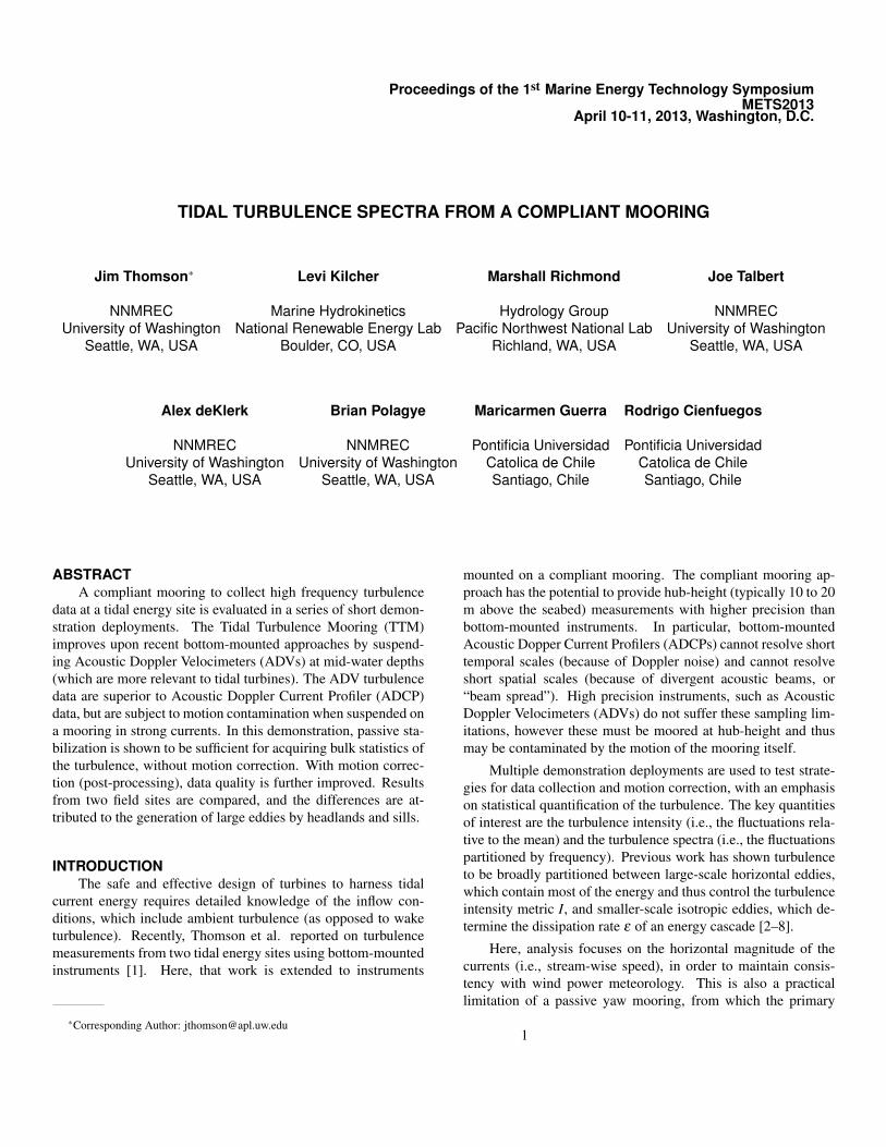
TIDAL TURBULENCE SPECTRA FROM A COMPLIANT MOORING

Jim Thomson∗

NNMRECUniversity of Washington

Seattle, WA, USA

Levi Kilcher

Marine HydrokineticsNational Renewable Energy Lab

Boulder, CO, USA

Marshall Richmond

Hydrology GroupPacific Northwest National Lab

Richland, WA, USA

Joe Talbert

NNMRECUniversity of Washington

Seattle, WA, USA

Alex deKlerk

NNMRECUniversity of Washington

Seattle, WA, USA

Brian Polagye

NNMRECUniversity of Washington

Seattle, WA, USA

Maricarmen Guerra

Pontificia UniversidadCatolica de ChileSantiago, Chile

Rodrigo Cienfuegos

Pontificia UniversidadCatolica de ChileSantiago, Chile

ABSTRACTA compliant mooring to collect high frequency turbulence

data at a tidal energy site is evaluated in a series of short demon-stration deployments. The Tidal Turbulence Mooring (TTM)improves upon recent bottom-mounted approaches by suspend-ing Acoustic Doppler Velocimeters (ADVs) at mid-water depths(which are more relevant to tidal turbines). The ADV turbulencedata are superior to Acoustic Doppler Current Profiler (ADCP)data, but are subject to motion contamination when suspended ona mooring in strong currents. In this demonstration, passive sta-bilization is shown to be sufficient for acquiring bulk statistics ofthe turbulence, without motion correction. With motion correc-tion (post-processing), data quality is further improved. Resultsfrom two field sites are compared, and the differences are at-tributed to the generation of large eddies by headlands and sills.

INTRODUCTIONThe safe and effective design of turbines to harness tidal

current energy requires detailed knowledge of the inflow con-ditions, which include ambient turbulence (as opposed to waketurbulence). Recently, Thomson et al. reported on turbulencemeasurements from two tidal energy sites using bottom-mountedinstruments [1]. Here, that work is extended to instruments

∗Corresponding Author: jthomson@apl.uw.edu

mounted on a compliant mooring. The compliant mooring ap-proach has the potential to provide hub-height (typically 10 to 20m above the seabed) measurements with higher precision thanbottom-mounted instruments. In particular, bottom-mountedAcoustic Dopper Current Profilers (ADCPs) cannot resolve shorttemporal scales (because of Doppler noise) and cannot resolveshort spatial scales (because of divergent acoustic beams, or“beam spread”). High precision instruments, such as AcousticDoppler Velocimeters (ADVs) do not suffer these sampling lim-itations, however these must be moored at hub-height and thusmay be contaminated by the motion of the mooring itself.

Multiple demonstration deployments are used to test strate-gies for data collection and motion correction, with an emphasison statistical quantification of the turbulence. The key quantitiesof interest are the turbulence intensity (i.e., the fluctuations rela-tive to the mean) and the turbulence spectra (i.e., the fluctuationspartitioned by frequency). Previous work has shown turbulenceto be broadly partitioned between large-scale horizontal eddies,which contain most of the energy and thus control the turbulenceintensity metric I, and smaller-scale isotropic eddies, which de-termine the dissipation rate ε of an energy cascade [2–8].

Here, analysis focuses on the horizontal magnitude of thecurrents (i.e., stream-wise speed), in order to maintain consis-tency with wind power meteorology. This is also a practicallimitation of a passive yaw mooring, from which the primary

1

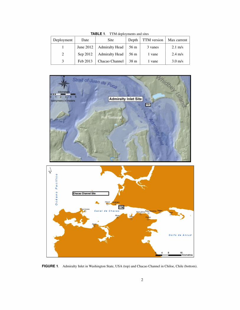
TABLE 1. TTM deployments and sites

Deployment Date Site Depth TTM version Max current

1 June 2012 Admiralty Head 56 m 3 vanes 2.1 m/s

2 Sep 2012 Admiralty Head 56 m 1 vane 2.4 m/s

3 Feb 2013 Chacao Channel 38 m 1 vane 3.0 m/s

FIGURE 1. Admiralty Inlet in Washington State, USA (top) and Chacao Channel in Chiloe, Chile (bottom).

2

measurement is always the stream-wise component. It is impor-tant to note that the variance of orthogonal components (a morecommon oceanographic description of turbulence) is larger thanthe variance of scalar speed. Higher-order moments, such as theskewness, kurtosis, and extreme values are not addressed here.

DATA COLLECTIONTo date, the Tidal Turbulence Mooring (TTM) has been de-

ployed three times: twice in Admiralty Inlet (Puget Sound, WA,USA) in 2012, and once in Chacao Channel (Chiloe, Chile) in2013. The deployments and sites are summarized in Table 1 andsite plan views are shown in Figure 1. Each deployment was onlya few days in duration, because the tidal harmonic characteriza-tion of these sites has already been conducted using multi-monthdeployments (e.g. [9]).

Site descriptionsThe first deployment was from 17:30 PDT on 12 Jun 2012 to

14:30 PDT on 14 Jun 2012 at N 48 09.171’, W 122 41.149’ nearAdmiralty Head, Puget Sound WA (USA). The site is approx-imately 56 m deep (relative to mean lower low water, MLLW)and the TTM deployment target depth was the nominal 10-m hubheight of the Open Hydro turbines (2 total) that are planned to bedeployed nearby in 2014, as a pilot project by Snohomish PublicUtility District. The TTM deployment was within 10 m, hori-zontally, of the sea-spider deployment for the turbulence mea-surements in [1]. A second deployment from 12:45 PDT on 19Sep 2012 to 14:45 on 20 Sep 2012 was conducted to assess thequality of passive acoustic (hydrophone) data collection as an-other potentional use of the TTM.

The third deployment was from 14:30 on 11 Feb 2013 to10:00 on 14 Feb 2013 in the vicinity of S 41 45.7’ W 73 40.9’near Carelmapu in the Chacao Channel, Chile. The site is ap-proximately 38 m deep (rel. MLLW) and the TTM deploymenttargeted the nominal 10-m hub height of an Open Hydro turbine(for consistency with the Admiralty measurements).

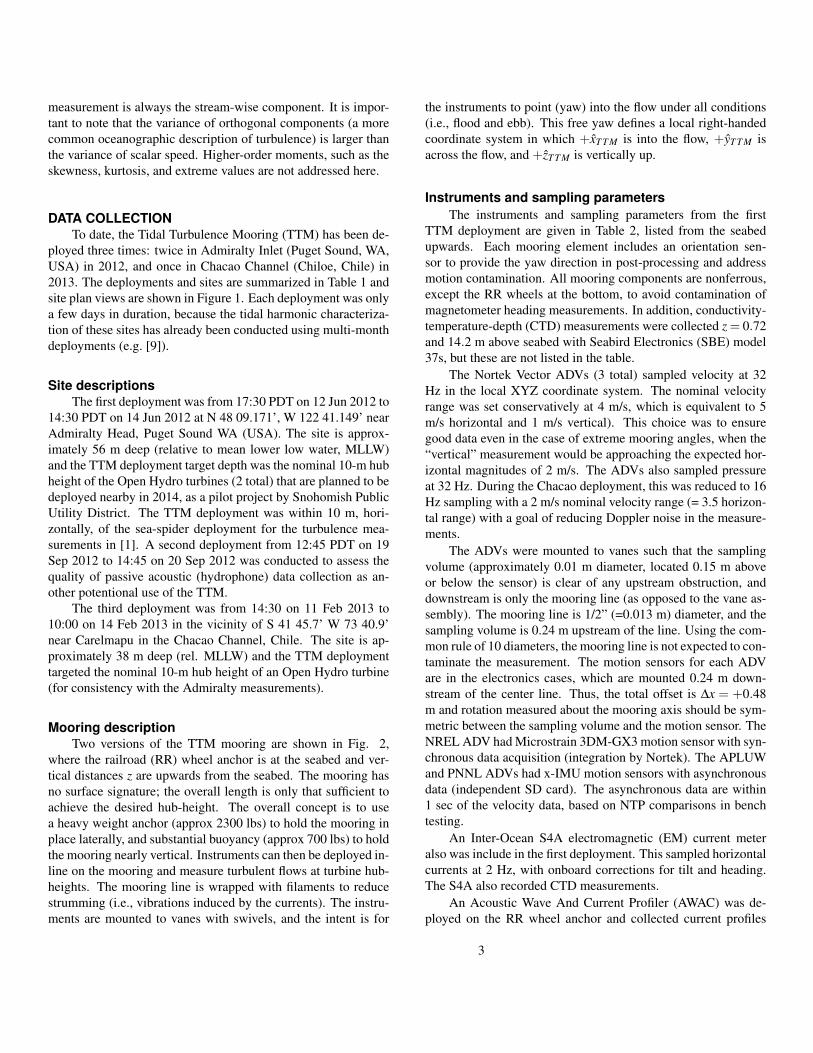
Mooring descriptionTwo versions of the TTM mooring are shown in Fig. 2,

where the railroad (RR) wheel anchor is at the seabed and ver-tical distances z are upwards from the seabed. The mooring hasno surface signature; the overall length is only that sufficient toachieve the desired hub-height. The overall concept is to usea heavy weight anchor (approx 2300 lbs) to hold the mooring inplace laterally, and substantial buoyancy (approx 700 lbs) to holdthe mooring nearly vertical. Instruments can then be deployed in-line on the mooring and measure turbulent flows at turbine hub-heights. The mooring line is wrapped with filaments to reducestrumming (i.e., vibrations induced by the currents). The instru-ments are mounted to vanes with swivels, and the intent is for

the instruments to point (yaw) into the flow under all conditions(i.e., flood and ebb). This free yaw defines a local right-handedcoordinate system in which +xT T M is into the flow, +yT T M isacross the flow, and +zT T M is vertically up.

Instruments and sampling parametersThe instruments and sampling parameters from the first

TTM deployment are given in Table 2, listed from the seabedupwards. Each mooring element includes an orientation sen-sor to provide the yaw direction in post-processing and addressmotion contamination. All mooring components are nonferrous,except the RR wheels at the bottom, to avoid contamination ofmagnetometer heading measurements. In addition, conductivity-temperature-depth (CTD) measurements were collected z = 0.72and 14.2 m above seabed with Seabird Electronics (SBE) model37s, but these are not listed in the table.

The Nortek Vector ADVs (3 total) sampled velocity at 32Hz in the local XYZ coordinate system. The nominal velocityrange was set conservatively at 4 m/s, which is equivalent to 5m/s horizontal and 1 m/s vertical). This choice was to ensuregood data even in the case of extreme mooring angles, when the“vertical” measurement would be approaching the expected hor-izontal magnitudes of 2 m/s. The ADVs also sampled pressureat 32 Hz. During the Chacao deployment, this was reduced to 16Hz sampling with a 2 m/s nominal velocity range (= 3.5 horizon-tal range) with a goal of reducing Doppler noise in the measure-ments.

The ADVs were mounted to vanes such that the samplingvolume (approximately 0.01 m diameter, located 0.15 m aboveor below the sensor) is clear of any upstream obstruction, anddownstream is only the mooring line (as opposed to the vane as-sembly). The mooring line is 1/2” (=0.013 m) diameter, and thesampling volume is 0.24 m upstream of the line. Using the com-mon rule of 10 diameters, the mooring line is not expected to con-taminate the measurement. The motion sensors for each ADVare in the electronics cases, which are mounted 0.24 m down-stream of the center line. Thus, the total offset is ∆x = +0.48m and rotation measured about the mooring axis should be sym-metric between the sampling volume and the motion sensor. TheNREL ADV had Microstrain 3DM-GX3 motion sensor with syn-chronous data acquisition (integration by Nortek). The APLUWand PNNL ADVs had x-IMU motion sensors with asynchronousdata (independent SD card). The asynchronous data are within1 sec of the velocity data, based on NTP comparisons in benchtesting.

An Inter-Ocean S4A electromagnetic (EM) current meteralso was include in the first deployment. This sampled horizontalcurrents at 2 Hz, with onboard corrections for tilt and heading.The S4A also recorded CTD measurements.

An Acoustic Wave And Current Profiler (AWAC) was de-ployed on the RR wheel anchor and collected current profiles

3

37" Steel Float ~700lbs Buoyancy

Nortek ADV, SBE 37

CTD, and 1 IMU on

strongback

ORE 8242 Acoustic Release

Nortek AWAC

5/8” SS Swivel

2 Nortek ADV’s and 2 IMU’s on

strongback

3 RR Wheel Anchor Stack ~ 2500lbs Wet

½” Amsteel Line

5/8" SAS

½” Galv Chain

½” Amsteel Line

½” Amsteel Line

½” Amsteel Line

3 Ton Esmet Swivel

IntercOcean S4A

Current Meter w/CTD

Water Depth: 55M

University of Washington

Applied Physics Laboratory

1013 NE 40th St.

Seattle, WA 98105

Joe Talbert

Tidal Turbulence Mooring

V2 pg 1

Location: Admialty Head

Deploy:6/12/12 Date: 4/17/12

SBE37

AWAC Battery

3 Ton Esmet Swivel

5/8" SAS

5/8" SS Shackle

5/8" SAS

5/8" SS Shackle

5/8" SS Shackle

5/8" SS Shackle

5/8" SS Shackle

5/8" SS Shackle

5/8" SAS

5/8" SAS

Drop Link

10M

5M

4M

7-12M off Bottom with

~20Degree Blowdown

FIGURE 2. Dimensional drawings of Tidal Turbulence Moorings deployed in Admiralty Inlet (left) and Chacao Channel (right).

every 1 s at 1 m resolution from 1.1 to 20.1 m above the seabed.The resulting AWAC Doppler noise of 0.112 m/s must be re-moved from statistical descriptions of the turbulence (see [1]).The AWAC recorded velocities in a magnetic East-North-Up(ENU) coordinate frame, using the standard onboard compassheading. Since the RR wheels are common steel, the compass

heading output may be biased, and resulting current directionsmust be validated against previous measurements at the site. An-other data quality concern is the potential interference of the up-per mooring elements, which may intersect the AWAC beamsduring large mooring angles. (When the mooring is purely ver-tical, under slack water conditions, the beam divergence of 25◦

4

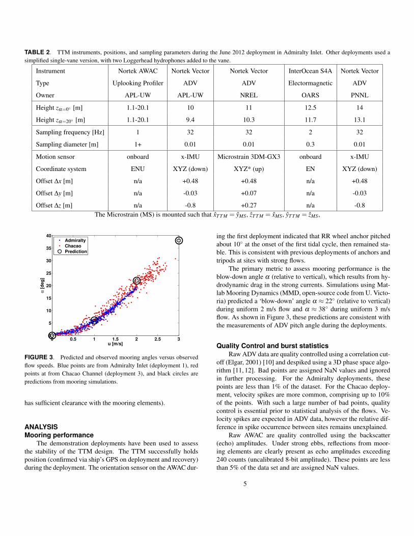
TABLE 2. TTM instruments, positions, and sampling parameters during the June 2012 deployment in Admiralty Inlet. Other deployments used asimplified single-vane version, with two Loggerhead hydrophones added to the vane.

Instrument Nortek AWAC Nortek Vector Nortek Vector InterOcean S4A Nortek Vector

Type Uplooking Profiler ADV ADV Electormagnetic ADV

Owner APL-UW APL-UW NREL OARS PNNL

Height zα=0◦ [m] 1.1-20.1 10 11 12.5 14

Height zα=20◦ [m] 1.1-20.1 9.4 10.3 11.7 13.1

Sampling frequency [Hz] 1 32 32 2 32

Sampling diameter [m] 1+ 0.01 0.01 0.3 0.01

Motion sensor onboard x-IMU Microstrain 3DM-GX3 onboard x-IMU

Coordinate system ENU XYZ (down) XYZ* (up) EN XYZ (down)

Offset ∆x [m] n/a +0.48 +0.48 n/a +0.48

Offset ∆y [m] n/a -0.03 +0.07 n/a -0.03

Offset ∆z [m] n/a -0.8 +0.27 n/a -0.8The Microstrain (MS) is mounted such that xT T M = yMS, zT T M = xMS, yT T M = zMS,

0 0.5 1 1.5 2 2.5 30

5

10

15

20

25

30

35

40

u [m/s]

α [

deg

]

Admiralty

Chacao

Prediction

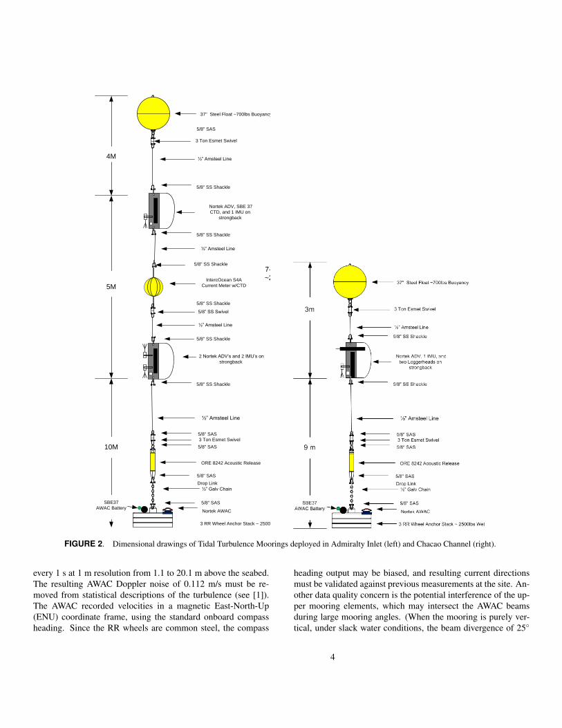
FIGURE 3. Predicted and observed mooring angles versus observedflow speeds. Blue points are from Admiralty Inlet (deployment 1), redpoints at from Chacao Channel (deployment 3), and black circles arepredictions from mooring simulations.

has sufficient clearance with the mooring elements).

ANALYSISMooring performance

The demonstration deployments have been used to assessthe stability of the TTM design. The TTM successfully holdsposition (confirmed via ship’s GPS on deployment and recovery)during the deployment. The orientation sensor on the AWAC dur-

ing the first deployment indicated that RR wheel anchor pitchedabout 10◦ at the onset of the first tidal cycle, then remained sta-ble. This is consistent with previous deployments of anchors andtripods at sites with strong flows.

The primary metric to assess mooring performance is theblow-down angle α (relative to vertical), which results from hy-drodynamic drag in the strong currents. Simulations using Mat-lab Mooring Dynamics (MMD, open-source code from U. Victo-ria) predicted a ‘blow-down’ angle α ≈ 22◦ (relative to vertical)during uniform 2 m/s flow and α ≈ 38◦ during uniform 3 m/sflow. As shown in Figure 3, these predictions are consistent withthe measurements of ADV pitch angle during the deployments.

Quality Control and burst statisticsRaw ADV data are quality controlled using a correlation cut-

off (Elgar, 2001) [10] and despiked using a 3D phase space algo-rithm [11, 12]. Bad points are assigned NaN values and ignoredin further processing. For the Admiralty deployments, thesepoints are less than 1% of the dataset. For the Chacao deploy-ment, velocity spikes are more common, comprising up to 10%of the points. With such a large number of bad points, qualitycontrol is essential prior to statistical analysis of the flows. Ve-locity spikes are expected in ADV data, however the relative dif-ference in spike occurrence between sites remains unexplained.

Raw AWAC are quality controlled using the backscatter(echo) amplitudes. Under strong ebbs, reflections from moor-ing elements are clearly present as echo amplitudes exceeding240 counts (uncalibrated 8-bit amplitude). These points are lessthan 5% of the data set and are assigned NaN values.

5

Velocity data are processed in five-minute bursts, follow-ing [1], such that stationarity is achieved and the changes in thetide do not affect the variance of the burst. Turbulence intensitiesare calculated from the stream-wise velocity component usingthe ratio of velocity standard deviation σu to velocity mean u.Doppler noise removal is negligible for ADV data. (This is incontrast to ADCP or AWAC data, in which Doppler noise re-moval is essential.) Turbulence spectra are calculated using theFFT of 128 s windows which are tapered with a Hamming win-dow, overlapped 50%, and then merged to obtain spectra with12 degrees of freedom. Later, these spectra are binned by meanvelocity to obtain characteristic spectra with approximately 96degrees of freedom each.

Motion correctionMotion correction for the ADV data requires accurate mea-

surements of mooring accelerations~a and spatial translation fromthe location of the motion sensor to the velocity ~u sampling vol-ume (see offsets in Table 2). Motion correction can be donedirectly for every point in a time series, or it can be done sta-tistically using frequency spectra. Here, we focus on horizontalmotions along the principal axis of the tidal flows (−x, in themooring reference frame, which yaws to face the mean currenton ebb and flood). First, an initial correction is made, based onburst-averaged mooring angle α , to obtain an approximately hor-izontally stream-wise velocity u. Then, correction for variationsin mooring orientation are applied.

Direct motion correction requires coherent (synchronous)data acquisition between raw velocity measurements uraw, moor-ing accelerations a, and mooring rotation ω , such that true ve-locities in the mooring reference frame (facing the flow) can beobtained at every time step t via displacement and rotation:

~u(t) =~uADV +~ω ×~l +∫~a ·dt, (1)

where ~l is the offset between the motion measurement and thevelocity measurement.

Spectral motion correction, by contrast, is statistical. Sinceacceleration is a = du

dt and frequency is f = ddt , the contami-

nation of motion (mooring accelerations) from turbulence fre-quency spectra can be removed via

T KE( f ) = Suu ± 2Xau f−1 − Saa f−2 (2)

where the analysis is restricted to the principal axis (x). Suu andSaa are the auto-spectra of the ADV data and the accelerations,respectively, and the cross-spectra term Xau arises because moor-ing motion and raw velocity observations are not independent.Rather, velocities are correlated with mooring motion. This is

10−2 10−1 100 101

10−4

10−3

10−2

10−1

100

Raw ADV

frequency [Hz]

S uu [m

2 s−2

/HZ]

f−5/3

<u>

[m/s

]

0.3

0.6

0.9

1.2

1.5

1.8

10−2 10−1 100 101

10−4

10−3

10−2

10−1

100

Acceleration

frequency [Hz]

S aa [m

2 s−4

/HZ]

<u>

[m/s

]

0.3

0.6

0.9

1.2

1.5

1.8

10−2 10−1 100 101

10−4

10−3

10−2

10−1

100

True TKE

frequency [Hz]

TKE

[m2 s

−2/H

Z]

f−5/3

<u>

[m/s

]0.3

0.6

0.9

1.2

1.5

1.8

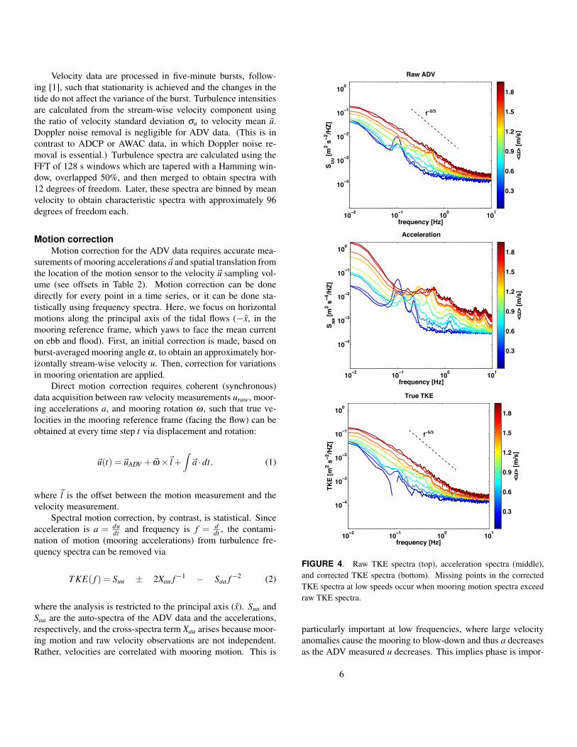
FIGURE 4. Raw TKE spectra (top), acceleration spectra (middle),and corrected TKE spectra (bottom). Missing points in the correctedTKE spectra at low speeds occur when mooring motion spectra exceedraw TKE spectra.

particularly important at low frequencies, where large velocityanomalies cause the mooring to blow-down and thus a decreasesas the ADV measured u decreases. This implies phase is impor-

6

00 01 02−3

−2

−1

0

1

2

3

u [

m/s

]

Admiralty

Chacao

00 01 020

5

10

15

20

Days of deployment

I [%

]

Admiralty

Chacao

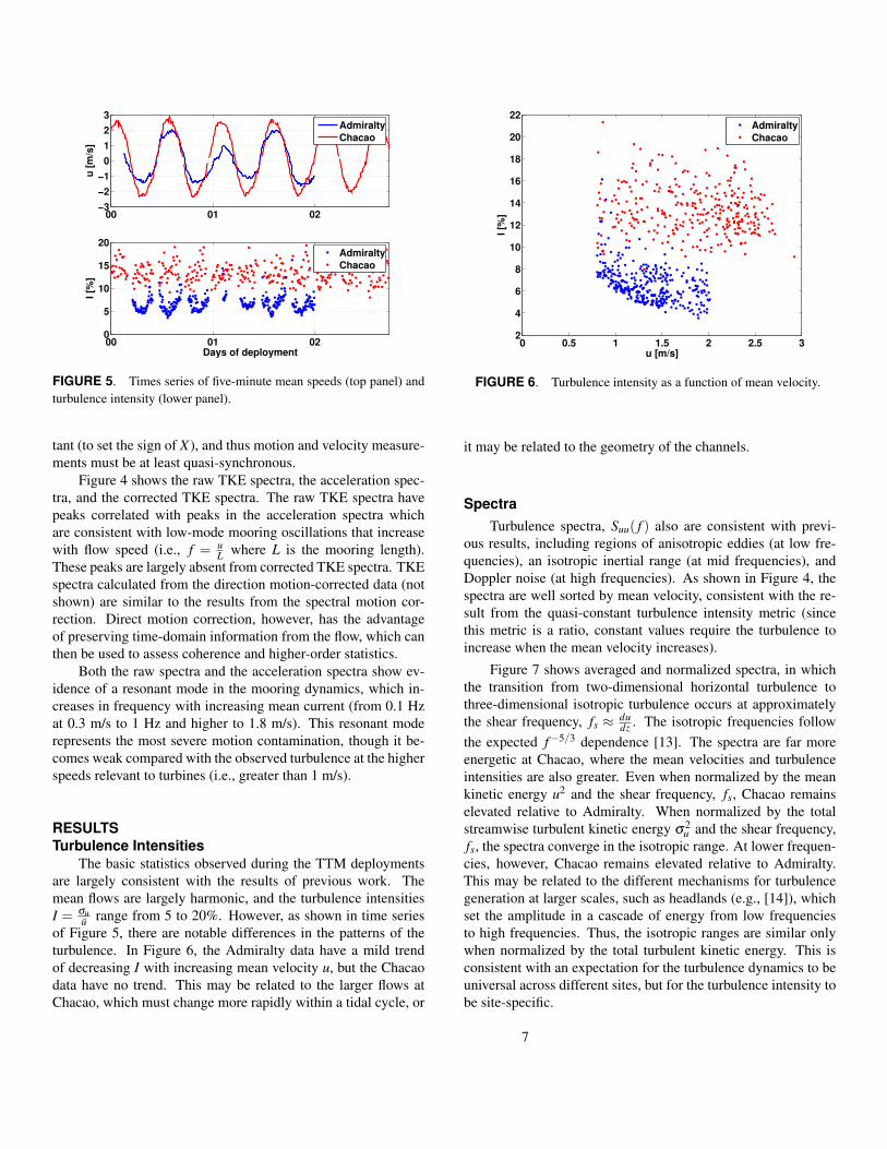
FIGURE 5. Times series of five-minute mean speeds (top panel) andturbulence intensity (lower panel).

tant (to set the sign of X), and thus motion and velocity measure-ments must be at least quasi-synchronous.

Figure 4 shows the raw TKE spectra, the acceleration spec-tra, and the corrected TKE spectra. The raw TKE spectra havepeaks correlated with peaks in the acceleration spectra whichare consistent with low-mode mooring oscillations that increasewith flow speed (i.e., f = u

L where L is the mooring length).These peaks are largely absent from corrected TKE spectra. TKEspectra calculated from the direction motion-corrected data (notshown) are similar to the results from the spectral motion cor-rection. Direct motion correction, however, has the advantageof preserving time-domain information from the flow, which canthen be used to assess coherence and higher-order statistics.

Both the raw spectra and the acceleration spectra show ev-idence of a resonant mode in the mooring dynamics, which in-creases in frequency with increasing mean current (from 0.1 Hzat 0.3 m/s to 1 Hz and higher to 1.8 m/s). This resonant moderepresents the most severe motion contamination, though it be-comes weak compared with the observed turbulence at the higherspeeds relevant to turbines (i.e., greater than 1 m/s).

RESULTSTurbulence Intensities

The basic statistics observed during the TTM deploymentsare largely consistent with the results of previous work. Themean flows are largely harmonic, and the turbulence intensitiesI = σu

u range from 5 to 20%. However, as shown in time seriesof Figure 5, there are notable differences in the patterns of theturbulence. In Figure 6, the Admiralty data have a mild trendof decreasing I with increasing mean velocity u, but the Chacaodata have no trend. This may be related to the larger flows atChacao, which must change more rapidly within a tidal cycle, or

0 0.5 1 1.5 2 2.5 32

4

6

8

10

12

14

16

18

20

22

u [m/s]

I [%

]

Admiralty

Chacao

FIGURE 6. Turbulence intensity as a function of mean velocity.

it may be related to the geometry of the channels.

SpectraTurbulence spectra, Suu( f ) also are consistent with previ-

ous results, including regions of anisotropic eddies (at low fre-quencies), an isotropic inertial range (at mid frequencies), andDoppler noise (at high frequencies). As shown in Figure 4, thespectra are well sorted by mean velocity, consistent with the re-sult from the quasi-constant turbulence intensity metric (sincethis metric is a ratio, constant values require the turbulence toincrease when the mean velocity increases).

Figure 7 shows averaged and normalized spectra, in whichthe transition from two-dimensional horizontal turbulence tothree-dimensional isotropic turbulence occurs at approximatelythe shear frequency, fs ≈ du

dz . The isotropic frequencies followthe expected f−5/3 dependence [13]. The spectra are far moreenergetic at Chacao, where the mean velocities and turbulenceintensities are also greater. Even when normalized by the meankinetic energy u2 and the shear frequency, fs, Chacao remainselevated relative to Admiralty. When normalized by the totalstreamwise turbulent kinetic energy σ2

u and the shear frequency,fs, the spectra converge in the isotropic range. At lower frequen-cies, however, Chacao remains elevated relative to Admiralty.This may be related to the different mechanisms for turbulencegeneration at larger scales, such as headlands (e.g., [14]), whichset the amplitude in a cascade of energy from low frequenciesto high frequencies. Thus, the isotropic ranges are similar onlywhen normalized by the total turbulent kinetic energy. This isconsistent with an expectation for the turbulence dynamics to beuniversal across different sites, but for the turbulence intensity tobe site-specific.

7

10−2

100

10−4

10−2

100

f [Hz]

Su

u [

m2/s

2 H

z−

1]

Dimensional

f−5/3

Admiralty

Chacao

10−2

100

f/fs

Su

u f

s / u

2

u2 scaled

10−2

100

f/fs

Su

u f

s / σ

u2

σu

2 scaled

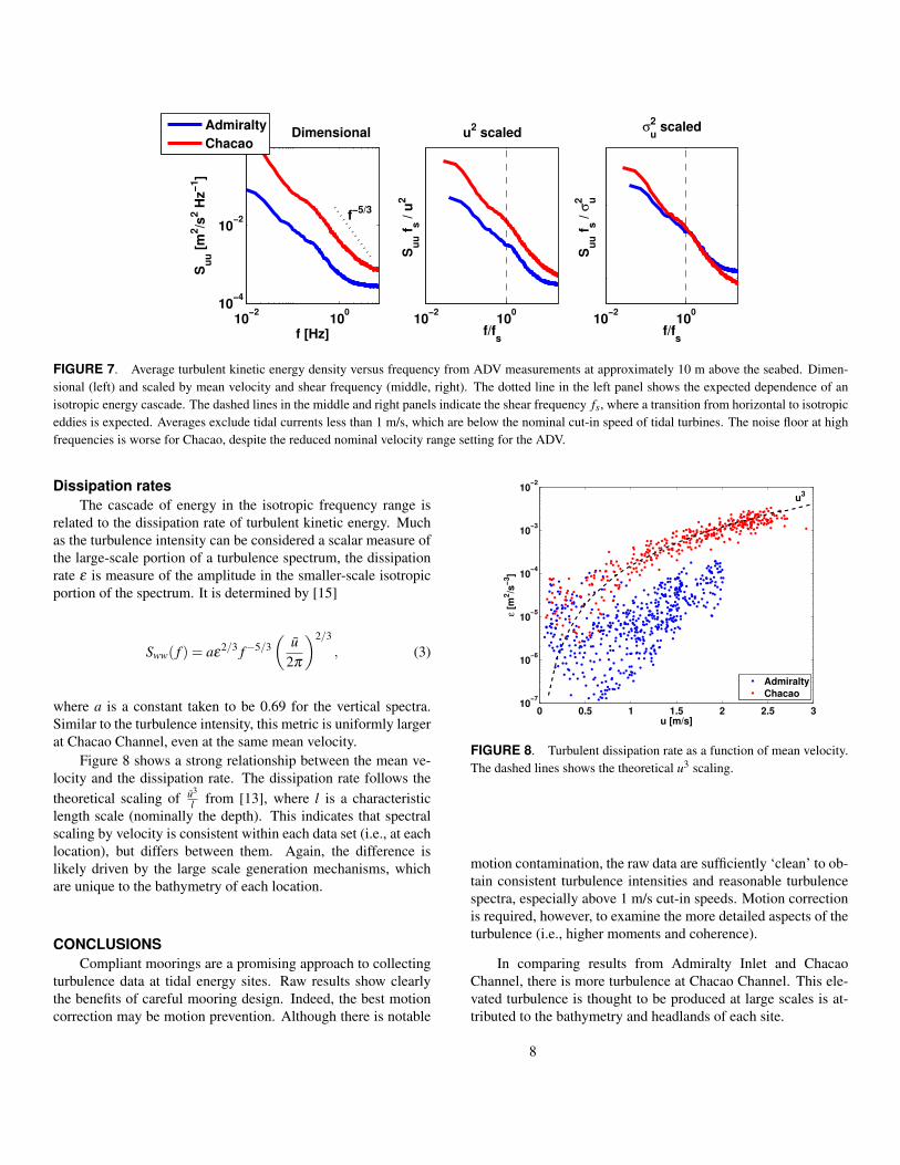
FIGURE 7. Average turbulent kinetic energy density versus frequency from ADV measurements at approximately 10 m above the seabed. Dimen-sional (left) and scaled by mean velocity and shear frequency (middle, right). The dotted line in the left panel shows the expected dependence of anisotropic energy cascade. The dashed lines in the middle and right panels indicate the shear frequency fs, where a transition from horizontal to isotropiceddies is expected. Averages exclude tidal currents less than 1 m/s, which are below the nominal cut-in speed of tidal turbines. The noise floor at highfrequencies is worse for Chacao, despite the reduced nominal velocity range setting for the ADV.

Dissipation ratesThe cascade of energy in the isotropic frequency range is

related to the dissipation rate of turbulent kinetic energy. Muchas the turbulence intensity can be considered a scalar measure ofthe large-scale portion of a turbulence spectrum, the dissipationrate ε is measure of the amplitude in the smaller-scale isotropicportion of the spectrum. It is determined by [15]

Sww( f ) = aε2/3 f−5/3

(u

2π

)2/3

, (3)

where a is a constant taken to be 0.69 for the vertical spectra.Similar to the turbulence intensity, this metric is uniformly largerat Chacao Channel, even at the same mean velocity.

Figure 8 shows a strong relationship between the mean ve-locity and the dissipation rate. The dissipation rate follows thetheoretical scaling of u3

l from [13], where l is a characteristiclength scale (nominally the depth). This indicates that spectralscaling by velocity is consistent within each data set (i.e., at eachlocation), but differs between them. Again, the difference islikely driven by the large scale generation mechanisms, whichare unique to the bathymetry of each location.

CONCLUSIONSCompliant moorings are a promising approach to collecting

turbulence data at tidal energy sites. Raw results show clearlythe benefits of careful mooring design. Indeed, the best motioncorrection may be motion prevention. Although there is notable

0 0.5 1 1.5 2 2.5 310

−7

10−6

10−5

10−4

10−3

10−2

u3

u [m/s]

ε [

m2/s

−3]

Admiralty

Chacao

FIGURE 8. Turbulent dissipation rate as a function of mean velocity.The dashed lines shows the theoretical u3 scaling.

motion contamination, the raw data are sufficiently ‘clean’ to ob-tain consistent turbulence intensities and reasonable turbulencespectra, especially above 1 m/s cut-in speeds. Motion correctionis required, however, to examine the more detailed aspects of theturbulence (i.e., higher moments and coherence).

In comparing results from Admiralty Inlet and ChacaoChannel, there is more turbulence at Chacao Channel. This ele-vated turbulence is thought to be produced at large scales is at-tributed to the bathymetry and headlands of each site.

8

ACKNOWLEDGMENTThanks to Capt. Andy Reay-Ellers ship operations in Admi-

ralty Inlet and Eduardo Hernandez for ship operations in Chacao.Thanks to Chris Bassett for the addition of passive acoustics tothe moorings. Support for this research provided by the U.S. De-partment of Energy and by the Office of Naval Research - Global.

REFERENCES[1] Thomson, J., Polagye, B., Durgesh, V., and Richmond, M.,

2012. “Measurements of turbulence at two tidal energysites in Puget Sound, WA”. J. Ocean. Eng., 37(3), pp. 363–374.

[2] Lu, Y., and Lueck, R. G., 1999. “Using a broadband ADCPin a tidal channel. part ii: Turbulence”. J. Atmos. Ocean.Tech., 16, pp. 1568–1579.

[3] Stacey, M. T., Monismith, S. G., and Burau, J. R., 1999.“Observations of turbulence in a partially stratified estu-ary”. J. Phys. Oceanogr., 29, pp. 1950–1970.

[4] Stacey, M., 2003. “Estimation of diffusive transport of tur-bulent kinetic energy from acoustic Doppler current profilerdata”. J. Atmos. Ocean. Tech., 20, pp. 927–935.

[5] Rippeth, T. P., Simpson, J. H., Williams, E., and Inall,M. E., 2003. “Measurements of the rates of production anddissipation of turbulent kinetic energy in an energetic tidalflow: Red Warf Bay revisited.”. J. Phys. Oceanogr., 33,pp. 1889–1901.

[6] Williams, E., and Simpson, J. H., 2004. “Uncertainties inestimates of Reynolds stress and TKE production rate usingthe adcp variance method”. J. Atmos. Ocean. Tech., 21,pp. 347–357.

[7] Wiles, P., Rippeth, T. P., Simpson, J., and Hendricks, P.,2006. “A novel technique for measuring the rate of turbu-lent dissipation in the marine environment”. Geophys. Res.Let., 33, p. L21608.

[8] Walter, R. K., Nidzieko, N. J., and Monismith, S. G., 2011.“Similarity scaling of turbulence spectra and cospectra in ashallow tidal flow”. J. Geophys. Res., 116(C10019).

[9] Polagye, B., and Thomson, J., 2013. “Tidal energy resourcecharacterization: methodolgy and field study in AdmiraltyInlet, Puget Sound, USA”. Proc. IMechE, Part A: J. Powerand Energy.

[10] Elgar, S., Raubenheimer, B., and Guza, R. T., 2001. “Cur-rent meter performance in the surf zone”. J. Atmos. Ocean.Tech., 18, pp. 1735–1746.

[11] Goring, D. G., and Nikora, V. I., 2002. “Despiking acous-tic doppler velocimeter data”. J. Hydraul. Eng, 128(1),pp. 117–126.

[12] Mori, N., Suzuki, T., and Kakuno, S., 2007. “Noise ofacoustic doppler velocimeter data in bubbly flow”. ASCEJournal of Engineering Mechanics, 133(1), pp. 122–125.

[13] Kolmogorov, A. N., 1941. “Dissipation of energy in the

locally isotropic turbulence”. Dokl. Akad. Nauk SSR, 30,pp. 301–305.

[14] Signell, R. P., and Geyer, W. R., 1991. “Transient eddyformation around headlands”. J. Geophys. Res., 96(C2),pp. 2561–2575.

[15] Lumley, J. L., and Terray, E. A., 1983. “Kinematics ofturbulence convected by a random wave field”. J. Phys.Oceanogr., 13, pp. 2000–2007.

9