turbulent flow

Turbulent Flow and Heat Transfer Problem in theElectromagnetic Continuous Casting Process

Theeradech Mookum, Benchawan Wiwatanapataphee, and Yong Hong Wu

Abstract— This paper aims to study the effect ofturbulence on the flow of two fluids and the heat transfer -solidification process in electromagnetic continuous steelcasting. The complete set of field equations is established.The flow pattern of the fluids, the meniscus shape andtemperature field as well as solidification profiles obtainedfrom the model with and with no turbulence effect arepresented. The results show that the model with turbulencegives a large circulation zone above the jet, much largervariation of the meniscus geometry, a slow solidificationrate and higher temperature in the top part of the strandregion.

Keywords— Electromagnetic continuous steel castingprocess, turbulent flow, heat transfer, two-fluid flow, levelset method.

I. INTRODUCTION

THE surface control of continuous steel castingproducts is important to steel quality. Over the

last decade, the technologies used to control thequality of the continuous casting products have beenproposed such as neural networks [23], fuzzy logic[24], optimization [27], and electromagnetic contin-uous casting process [10], [15]. The electromagneticsteel casting process is a relatively new effectiveheat extraction process in which molten steel iswithdrawn at a specified speed. In comparison withthe normal continuous casting process, the electro-magnetic continuous casting process possesses manyadvantages such as improving the surface quality,controlling the flow pattern of liquid steel, and re-moving the inclusions and gas bubbles [16], [28].

Manuscript received April 7, 2011; revised May 30, 2011.This work was supported by the Office of the Higher EducationCommission and the Thailand Research Fund through the RoyalGolden Jubilee Ph.D. Program (Grant No. PHD/0212/2549), andan Australia Research Council Discovery project grant.

T. Mookum is with School of Science, Mae Fah LuangUniversity, 333 Moo 1, Thasud, Muang, Chiang Rai 57100THAILAND (e-mail:[email protected]).

B. Wiwatanapataphee is with Department of Mathematics,Faculty of Science, Mahidol University, 272 Rama 6 Road,Rajthevee, Bangkok 10400 THAILAND (corresponding author;e-mail:[email protected]).

Y.H. Wu is with Department of Mathematics and Statistics,Curtin University of Technology, Perth, WA 6845 AUSTRALIA(e-mail:[email protected]).

Due to these advantages, great efforts have beenmade to develop this process over the last decadeand the percentage of steel in the world produced bythis process is increasing.

In the electromagnetic casting, a coil is mountedaround the casting mould. The magnetic field gener-ated from the source current through the coil inducesthe electric current in the steel pool. This currentnot only heats the molten steel but also generates anelectromagnetic force in the molten steel. During theprocess, the molten steel is poured from a ladle intoan intermediate container known as a tundish. Themolten steel from the tundish is transferred througha submerged entry nozzle into a water-cooled mould,where intense cooling causes a thin solidified steelshell to form around the edge of the steel, leavinga large molten core inside the shell. To facilitatethe process, mould powder or lubricant oil is addedat the top of the mould to prevent the steel fromoxidizing. The interface between the molten steeland lubricant oil is known as a “meniscus”. Themould is oscillated vertically and then the lubricantliquid is dragged into the gap between the solidifiedstrand and the mould walls. This can prevent thesteel from sticking to the solidifying shell. Afterleaving the mould, the solidified strand is supportedby a set of rollers, cooled down by water sprays andthen subsequently cooled through radiation. Whenthe casting has attained the desired length, it is cutoff with a cutter.

The electromagnetic field imposed to the processis the effective technology to control heat transportand solidification [2], [5], [20], [25], [26]. The elec-tromagnetic force can reduce the molten steel flowfrom hitting the wall [7], [28] and push the meniscusaway from the mould during casting [19], whichreduces the surface contact between the melt and thewall. The behavior of electromagnetic stirring, fluidflow, heat transfer with solidification and oscillationmarks on the steel surface is crucial to the qualityand productivity of the process. The effect of theelectromagnetic field on turbulent flow has also beeninvestigated [8], [6], [22], [28].

With the limitation of experiments in the contin-uous casting process, mathematical models becomean important tool to understand the physical phenom-

INTERNATIONAL JOURNAL OF MATHEMATICS AND COMPUTERS IN SIMULATION

Issue 4, Volume 5, 2011 310

ena. Over the last few decades, most of the researchefforts have been focussed on investigating the flowpattern and heat transfer problems in the continuouscasting process [1], [4], [7], [9], [11], [18], [21].Mookum [12], [13] presented a mathematical modelto study the effect of electromagnetic field on theflow and temperature fields. The results indicatedthat the electromagnetic force reduced the speedof the molten steel near the mould wall. Wu andWiwatanapataphee [29], [30] proposed a mathemat-ical model to solve the coupled turbulent two-fluidflow and heat transfer with solidification. However,many phenomena such as the heat transfer process,the formation of oscillation marks and the meniscusbehavior, have not been fully understood nor wellcontrolled.

In this study, we extend the previous work [14]and propose a three-dimensional mathematical modelfor the problem of turbulent two-fluid flow and heattransfer with solidification in the electromagneticcontinuous steel casting process. The effect of turbu-lent flow on temperature distribution and meniscussurface is investigated. The rest of the paper isorganized as follows. In section two, a completeset of field equations and finite element formulationare given. Section three gives a numerical study todemonstrate the effect of electromagnetic force onthe flow pattern, the heat transfer and solidificationprocess as well as the meniscus shape.

II. MATHEMATICAL MODELS

A. Governing EquationsIn this work, we study the effect of the electro-

magnetic force on the turbulent flow of fluids in thecontinuous steel casting process. In the mould region,there are two immiscible fluids, namely molten steelregion (Ωs) and lubricant oil region (Ωo). To studythe motion of the two fluids, we introduce the levelset function ϕ as

ϕ(xi, t) =

0 if xi ∈ Ωs

0.5 if xi ∈ Γint

1 if xi ∈ Ωo,

(1)

where Γint is the interface between the molten steeland the lubricant oil. Using ϕ, we can define thedensity, ρ, and the viscosity, µ, as follows:

ρ = ρs + (ρo − ρs)ϕ, (2)

µ = µs + (µo − µs)ϕ, (3)

where the subscripts s and o denote respectively themolten steel and lubricant oil.

The velocity and pressure fields described by theincompressible Navier-Stokes equations for the two-fluid flow are given below

∂ui∂xi

= 0, (4)

ρ

(∂ui∂t

+ uj∂ui∂xj

)+∂p

∂xi− ∂

∂xj

(µeff

(∂ui∂xj

+∂uj∂xi

))= ρgi + Femi

+ Fsti + Fi(ui, xi, t), (5)

where ui represents the velocity of the fluids, p isthe fluid pressure, gi is the gravitational acceleration,Femi

is the electromagnetic force, Fsti is the surfacetension force and Fi is the forcing function.

To solve equations (4) and (5), we need tocouple the two-fluid flow problem with the heattransfer problem. Based on the enthalpy formulation,the temperature field is governed by the followingequation:

ρc

(∂T

∂t+ uj

∂T

∂xj

)=

∂

∂xj

(keff

∂T

∂xj

)− ρs

(∂HL

∂t+ uj

∂HL

∂xj

)(1− ϕ), (6)

where T is the temperature, HL is the laten heatdefined as HL = Lf(T ) in which L represents thelatent heat of liquid steel. The liquid fraction f(T )is given by

f(T ) =

0 if T ≤ TS ,T − TSTL − TS

if TS < T < TL,

1 if T ≥ TL,

(7)

where TS and TL are the solidification temperatureand melting temperature of the steel, respectively.The thermal conductivity, k, and the heat capacity,c, are expressed in terms of ϕ as follows:

k = ks + (ko − ks)ϕ, (8)

c = cs + (co − cs)ϕ. (9)

The effective viscosity, µeff , and the effectivethermal conductivity, keff , in equations (5) and (6),respectively, are given by

µeff = µ+ µt, keff = k +cµtσt, (10)

where σt is the turbulence Prandtl number assumedas 0.9 [1]. The turbulent viscosity, µt, is determinedby

µt = ρCµK2

ε. (11)

The coefficient Cµ is suggested to be 0.09 [9], Kis the turbulent kinetic energy and ε is the turbulent



dissipation rate. The two-equation K − ε model isused to study the effect of turbulence on the velocityand temperature fields, namely

ρ

(∂K

∂t+ uj

∂K

∂xj

)=

∂

∂xj

[(µ+

µtσK

)∂K

∂xj

]−µtσtβgi

∂T

∂xi+ µtG− ρε

(12)

ρ

(∂ε

∂t+ uj

∂ε

∂xj

)=

∂

∂xj

[(µ+

µtσε

)∂ε

∂xj

]+C1(1− C3)

εµtKσt

βgi∂T

∂xi+ C1ε

µtKG− C2ρ

ε2

K(13)

where G =∂ui∂xj

(∂ui∂xj

+∂uj∂xi

), β is the thermal

expansion of steel, the coefficients C1 = 1.44, C2 =1.92, σK = 1 and σε = 1.3 [9].

To determine the movement of the interface, thelevel set function is obtained by solving the followingequation [17]:

∂ϕ

∂t+ uj

∂ϕ

∂xj= γ

∂

∂xj

(ϵ∂ϕ

∂xj− ϕ(1− ϕ)nj

).

(14)The quantities γ and ϵ are reinitialization parameterand thickness of the interface. The reinitialization ofequation (14) is given by

∂ϕ

∂t= γ

∂

∂xj

(ϵ∂ϕ


). (15)

The equation (15) is first solved to obtain the initialcondition for the level set equation (14).

Based on our previous work in [12], the electro-magnetic force can be determined by

Fem = J × (∇× A), (16)

where J and A denote the total current densityand the magnetic vector potential, respectively. Toobtain the electromagnetic force, the magnetic vectorpotential A and the scalar potential φ are determinedfrom Maxwell’s equations by

∇ · (−η∇φ+ Js) = 0, (17)

−1

ν∇2A + ηιωA = −η∇φ+ Js, (18)

where Js is the source current density, η is theelectric conductivity, ν is the magnetic permeability,ω is the current frequency, and ι =

√−1.

The surface tension force in equation (5) con-centrated around the interface can be expressed as

Fst = σκ(ϕ)δ(ϕ)n, (19)

where σ, n, and κ are respectively the surface ten-sion coefficient, the interface normal vector, and theinterfacial curvature. The quantities n, and κ arecalculated by n = ∇ϕ

|∇ϕ| and κ(ϕ) = −∇ · n. Thedelta function δ(ϕ) employed in this study is givenby [3]

δ(ϕ) = 6|∇ϕ||ϕ(1− ϕ)|. (20)

The forcing function F (u,x, t) in equation (5)is determined, according to [1], by

F (u,x, t) = Cµt(1− f(T ))2

f(T )3(u−U cast), (21)

where U cast = (0, 0, Ucast) in which Ucast repre-sents the constant downward casting speed and C isthe morphology constant.

To completely define the problem, a set ofboundary conditions have been established to sup-plement the above field equations and are shown inFig. 2.

Fig. 1. Computation domain

B. Finite Element FormulationIn this study, we employ a Bubnov-Galerkin fi-

nite element method for the numerical simulation andinvestigation. The electromagnetic force in equation(16) is obtained first by solving the electromagneticfield in equations (17) and (18). In order to obtain



Fig. 2. Boundary conditions

the finite element solution of Ai and φ, the varia-tional problem for the equations (17) and (18) areestablished:

Find φ,Ai ∈ H1(Ω) such that for all testfunctions wb, wc

i ∈ H10 (Ω), the relevant Dirichlet

type boundary conditions are satisfied and∫Ωwb ∂

∂xj

(−η ∂φ

∂xj+ Js

j

)dΩ = 0, (22)

−∫Ωwci

1

ν

∂2Ai

∂xj∂xjdΩ+

∫ΩwciηιωAidΩ

=

∫Ωwci

(−η ∂φ

∂xi+ Js

i

)dΩ, (23)

where H1(Ω) is the Sobolev space W 1,2(Ω) withnorm ∥ · ∥1,2,Ω, H1

0 (Ω) = v ∈ H1(Ω)|v = 0 onthe boundary. By using the Galerkin finite elementformulation, we obtain the following discretizationsystem

ηMφ = FJ , (24)(1

νM + ηιωB

)A = FA, (25)

where M and B are the coefficient matrices. To solvethe steady state system of equations (24) and (25),we can solve first equation (24) for φ and then usethis solution to solve equation (25) for A.

For the finite element solution of ui, p, T, ϕ,Kand ε, the variational statement for the boundary

value problem corresponding to the the equations (4),(5), (6), (12), (13), and (14) subjected to relevantboundary conditions is established as follows:

Find ui, p, T, ϕ,K, ε ∈ H1(Ω) such that forall wi, wp, wτ , wϕ, wK , wε ∈ H1

0 (Ω), all relevantDirichlet type boundary conditions are satisfied and∫

Ωwp∂uj∂xj

dΩ = 0, (26)

∫Ωwi∂ui

∂tdΩ+

∫Ωwi(uj

∂ui∂xj

)dΩ

−∫Ω

1

ρ

∂wi

∂xipdΩ+

∫Ω

µ

ρ

(∂wi

∂xj

∂ui∂xj

+∂wi

∂xi

∂uj∂xi

)dΩ

=

∫ΩwigidΩ+

∫Ω

1

ρwiFemi

dΩ

+

∫Ω

1

ρwiFstidΩ+

∫Γwall

µ

ρhwiuidΓ, (27)

∫Ωwτ ∂T

∂tdΩ+

∫Ωwτ (uj

∂T

∂xj)dΩ

+

∫Ω

k

ρc

∂wτ

∂xj

∂T

∂xjdΩ = −

∫Γwall

1

ρcwτh∞(T − Tm)dΓ

−∫Γstrand

1

ρcwτ

(h∞(T − T∞) + ςϖ(T 4 − T 4

ext))dΓ

−∫Ω

1

cswτ

(∂HL

∂t+ (uj

∂HL

∂xj)

)(1− ϕ)dΩ, (28)

∫Ωwϕ∂ϕ

∂tdΩ+

∫Ωwϕ(uj

∂ϕ

∂xj)dΩ

=

∫Ωwϕγ

∂

∂xj

(ε∂ϕ


)dΩ. (29)

∫ΩwKρ

∂K

∂tdΩ+

∫ΩwKuj

∂K

∂xjdΩ

=

∫ΩwK ∂

∂xj

[(µ+

µtσK

)∂K

∂xj

]dΩ

−∫ΩwK µt

σtβgi

∂T

∂xidΩ+

∫ΩwKµtGdΩ

−∫ΩwKρεdΩ (30)

∫Ωwερ

∂ε

∂tdΩ+

∫Ωwεuj

∂ε

∂xjdΩ

=

∫Ωwε ∂

∂xj

[(µ+

µtσε

)∂ε

∂xj

]dΩ

+

∫ΩwεC1(1− C3)

εµtKσt

βgi∂T

∂xidΩ

+

∫ΩwεC1ε

µtKGdΩ−

∫ΩwεC2ρ

ε2

KdΩ (31)



The above equations for(ux, uy, uz, p, T, ϕ,K, ε) are then discretized inspace by the level set finite element method toyield the following system of nonlinear ordinarydifferential equations

M U + BU = F, (32)

where U = uxi, uyi, uzi, pi, Ti,Ki, εiNi=1 are thevalue of ux, uy, uz, p, T, ϕ,K, and ε at the nodesof the finite element mesh. The coefficient matrixM corresponds to the transient terms in the gov-erning partial differential equations, the matrix Bcorresponds to the advection and diffusion terms, andthe vector F corresponds to the external body force.

To solve the system of ordinary differentialequations (32), the backward Euler scheme is em-ployed. The convergence criteria used for the itera-tive scheme is given by

∥Ri+1n −Ri

n∥ < Tol, (33)

where i + 1 and i denote the iterative computationsteps, Rn represents the unknown vector of the nthvariable on the finite element nodes, ∥ · ∥ denotesthe Euclidean norm and Tol is a very small positivenumber.

Fig. 3. Vector plot of the total current density on the front andtop view

III. NUMERICAL RESULTSFor numerical investigation, we consider a

square billet with a width of 0.2 m and a depth of 0.4m, and a submerged entry nozzle with port angle of12 downward. The inlet velocity of molten steel is0.12 m/s; the molten steel is assumed to have 5C of

Fig. 4. Vector plot of the electromagnetic force on the frontand top view

Fig. 5. The velocity fields under two different cases: (a) withturbulence effect;(b) with no turbulence effect

super-heat; and the delivery turbulent kinetic energyand its dissipation rate are respectively 0.0502 m2/s2

and 0.457 m2/s2. The values of other parameters aregiven in Table I. The computation domain shown inFig. 1 represents one quadrant of the casting steelsystem consisting of the strand region occupied bythe steel and lubricant oil on the top, the mouldregion, the coil region, and the environment region.The domain is discretized using 60,462 tetrahedralelements with a total of 625,737 degrees of freedom.

Fig. 3 shows the total current density J on thefront and top views. The result shows that the currentdensity concentrated around the edge of the mould



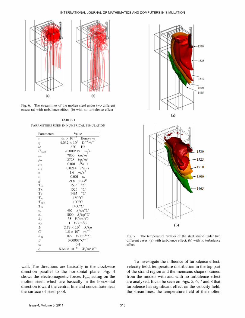
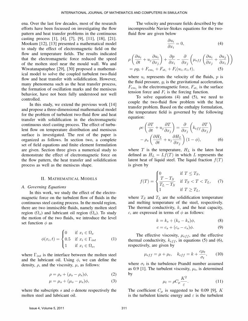
Fig. 6. The streamlines of the molten steel under two differentcases: (a) with turbulence effect; (b) with no turbulence effect

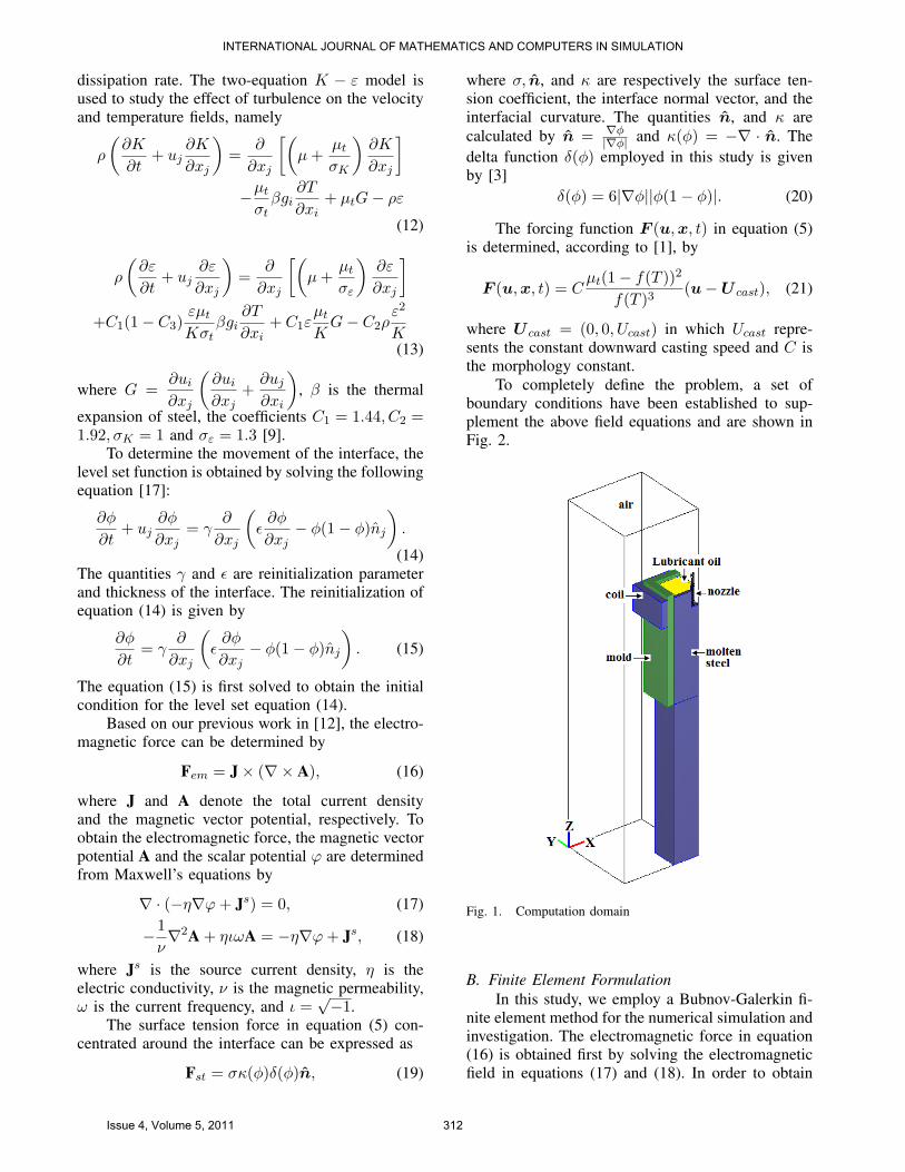
TABLE IPARAMETERS USED IN NUMERICAL SIMULATION

Parameters Valueν 4π × 10−7 Henry/mη 4.032× 106 Ω−1m−1

ω 320 HzUcast -0.000575 m/sρs 7800 kg/m3

ρo 2728 kg/m3

µs 0.001 Pa · sµo 0.0214 Pa · sσ 1.6 m/s2

ϵ 0.001 mg -9.8 m/s2

Tin 1535 oCTL 1525 oCTS 1465 oCT∞ 150oCText 100oCTm 1400oCcs 465 J/kgoCco 1000 J/kgoCks 35 W/moCko 1 W/moCL 2.72× 105 J/kgC 1.8× 106 m−2

h∞ 1079 W/m2oCβ 0.00003oC−1

ϖ 0.4ς 5.66× 10−8 W/m2K4

wall. The directions are basically in the clockwisedirection parallel to the horizontal plane. Fig. 4shows the electromagnetic forces Fem acting on themolten steel, which are basically in the horizontaldirection toward the central line and concentrate nearthe surface of steel pool.

Fig. 7. The temperature profiles of the steel strand under twodifferent cases: (a) with turbulence effect; (b) with no turbulenceeffect

To investigate the influence of turbulence effect,velocity field, temperature distribution in the top partof the strand region and the meniscus shape obtainedfrom the models with and with no turbulence effectare analyzed. It can be seen on Figs. 5, 6, 7 and 8 thatturbulence has significant effect on the velocity field,the streamlines, the temperature field of the molten



Fig. 8. The shape of the meniscus surface between the lubricantoil and the molten steel under two different cases: (a) withturbulence effect; (b) with no turbulence effect

steel, and the meniscus shape between the two fluids.The results show that under the turbulence condition,A large circulation zone presents above the jet asshown in Figs. 5(a) and 6(a), and molten steel startsto solidify at the bottom of the coil as shown inFig.7(a). In the model with no turbulence effect, tworecirculation zones above and below the jet appearas shown in Figs. 5(b) and 6(b), and molten steelstarts to solidified (T = 1465) at the top of the coilas shown in Fig. 7(a). The meniscus shape enlargedby flow is different as shown in Figs. 8(a-b). In themodel with no turbulence effect, meniscus shape isconcave along the mould wall and convex along thesymmetry plane. In the model with turbulence effect,the meniscus shape varies significantly in the liquidpool from the center to the edge of the steel strand.

IV. CONCLUDING REMARKSA three-dimensional mathematical model has

been developed to study the coupled turbulent two-fluid flow and heat transfer process in electromag-netic continuous steel casting. Turbulence effect onthe velocity field, temperature field, and meniscusshape has been investigated. The results show thatturbulence has significant effect on the velocity field,streamlines, temperature field of the molten steeland the meniscus shape between the two fluids. In

the model with no turbulence effect, there are tworecirculation zones respectively above and below thejet, and initial solidification of molten steel occursat the top of the coil, and the concave and convexshape of the meniscus appears along the mould walland convex along the symmetry plane, respectively.On the other hand, the model with turbulence gives alarge circulation zone above the jet, a slow solidifica-tion rate, and a large variation of the meniscus shape.It can be concluded that the model with turbulencegives much larger variation of the meniscus geometryand higher temperature in the top part of the strandregion.

ACKNOWLEDGMENT

The authors gratefully acknowledge the supportof the Office of the Higher Education Commis-sion and the Thailand Research Fund through theRoyal Golden Jubilee Ph.D. Program (Grant No.PHD/0212/2549), and an Australia Research CouncilDiscovery project grant.

REFERENCES[1] M.R. Aboutalebi, M. Hasan, and R.I.I. Guthrie, Coupled

turbulent flow, heat and solute transport in continuouscasting processes, Metall. Mater. Trans. vol.26B, 1995,pp. 731-744.

[2] P.R. Cha, Y.H. Hwang, H.S. Nam, S.H. Chung, andJ.K. Yoon, 3D numerical analysis on electromagnetic andfluid dynamic pheonomena in a soft contact electromag-netic slab caster, ISIJ Inter. vol.38, 1998, pp. 403-410.

[3] J.P.A. Bastos, and N. Sadowski, Comsol multiphysics mod-eling guide version 3.4, COMSOLAB 2007.

[4] J.H. Ferziger, Simulation of incompressible turbulent flow,Comput. Phys. vol.69, 1987, pp. 1-48.

[5] K. Fujisaki, In-mold electromagnetic stirring in continuouscasting, IEEE Trans. Industry Applications vol.37, No.4,2001, pp. 1098-1104.

[6] M.Y. Ha, H.G. Lee, and S.H. Seong, Numerical simulationof three-dimensional flow, heat transfer, and solificationof steel in continuous casting mold with electromagneticbrake, Metal. Mater. Inter. vol.133, 2003, pp. 322-339.

[7] K.G. Kang, H.S. Ryou, and N.K. Hur, Coupled turbu-lent flow, heat, and solute transport in continuous cast-ing process with an electromagnetic brake, Numer. HeatTrans. A. vol.48, 2005, pp. 461-481.

[8] D.S. Kim, W.S. Kim, and K.H. Cho, Numerical simulationof the coupled turbulent flow and macroscopic solidifi-cation in continuous casting with electromagnetic brake,ISIJ. Inter. vol.40, 2000, pp. 670-676.

[9] B.E. Launder and D.B. Spalding, The numerical computa-tion of turbulent flows, Comput. Meth. Appl. Mech. vol.3,1974, pp. 269-289.

[10] T.J. Li, K. Sassa, and S. Asai, Surface quality improvementof continuously cast metals by imposing intermittent highfrequency magnetic field and synchonysing the field withmold oscillation, ISIJ. Inter. vol.36, No.4, 1996, pp. 410-416.

[11] P.R. Lopez, R.D. Morales, R.S. Perez, and L.G. Demedices,Structure of turbulent flow in slab mold, Metall. Me-ter. Trans. B. vol.36B, 2005, pp. 787-800.



[12] T. Mookum, B. Wiwatanapataphee, and Y.H. Wu,Numerical simulation of three-dimensional fluid flowand heat transfer in electromagnetic steel casting,Int. J. Pure. Appl. Math vol.52, No.3, 2009, pp. 373-390.

[13] T. Mookum, B. Wiwatanapataphee, and Y.H. Wu, Model-ing of two-fluid flow and heat transfer with solidificationin continuous steel casting process under electromagneticforce, Int. J. Pure. Appl. Math vol.63, No.2, 2009, pp. 183-195.

[14] T. Mookum, B. Wiwatanapataphee, and Y.H. Wu, Theeffect of turbulence on two-fluid flow and heat transferin continuous steel casting process, Proceedings of the 4thWSEAS Int. Conf. on F-and-B’11. ISBN:978-960-474-298-1, 2011, pp. 53-58.

[15] H. Nakata, T. Inoue, H. Mori, K. Ayata, T. Murakami,and T. Kominami, Improvement of billet surface qualityby ultra-high frequency electromagnetic casting, ISIJ. In-ter. vol.42, 2002, pp. 246-272.

[16] T.T. Natarajan and N. El-Kaddah, Finite element analysisof electromagnetic and fluid flow phenomena in rotary elec-tromagnetic stirring of steel, Appl. Math. Model. vol.28,2004, pp. 47-61.

[17] E. Olssen, G. Kreiss, and S. Zahedi, A conservative levelset method for two phase flow II, J. Comput. Phys. Vol.225,2007, pp. 785-807.

[18] R. Sanchez-Perez, R.D. Morales, M. Dıaz-Cruz,O. Olivares-Xometl, and J. Palafox-Ramos, A physicalmodel for the two-phase flow in a nontinuous castingmold, ISIJ. Inter. vol.32, 1992, pp. 521-528.

[19] K. Takatani, K. Nakai, N. Kasai, T. Watanabe, andH. Nakajima, Analysis of heat transfer and fluid flow inthe continuous casting mold with electromagnetic brake,ISIJ Inter. vol.29, 1989, pp. 1063-1068.

[20] G.R. Tallback and J.D. Lavers, Influence of model param-eters on 3-D turbulent flow in an electromagnetic stirringsystem for continuous billet casting, IEEE Trans. Magnet-ics vol.40, No.2, 2004, pp. 597-600.

[21] B.G. Thomas, Continuous casting: complex models, Ency-clopedia of Materials: Science and Technology vol.2, 2001,pp. 1599-1609.

[22] X.Y. Tian, F. Zou, B.W. Li, and J.C. He, Numerical anal-ysis of coupled fluid flow, heat transfer and macroscopicsolidification in the thin slab funnel shape mold with anew type EMBr, Metall. Mater. Tran. B. vol.41B, 2009,pp. 112-120.

[23] G.O. Tirian and C. Pinca-Bretotean, Applications of neuralnetworks in continuous casting, WSEAS Trans. Sys. Vol.8,No.6, 2009, pp. 693-702.

[24] G.O. Tirian, C. Pinca-Bretotean, D. Cristea, and M. Topor,Applications of fuzzy logic in continuous casting,WSEAS Trans. Sys. Contr. Vol.5, No.3, 2010, pp. 133-142.

[25] T. Toh, E. Takeuchi, M. Hojo, H. Kawai, S. Matsumura,Electromagnetic control of initial solidification in continu-ous casting of steel by low frequency alternating magneticfield. ISIJ Inter. vol.37, 1997, pp. 1112-1119.

[26] L.B. Trindade, A.C.F. Vilela, A.F.F. Filho,M.T.M.B. Vilhena, and R.B. Soares, Numerical modelof electromagnetic stirring for continuous casting billets,IEEE Trans. Magnetics vol.38, No.6, 2002, pp. 3658-3660.

[27] M. Tufoi, I. Vela, C. Marta, D. Amariei, A.I. Tuta, andC. Mituletu, Optimization of withdrawing cylinder at ver-tical continuous casting of steel using CAD and CAE, Int.J. Mech. vol.5, No.1, 2011, pp. 10-18.

[28] Y.H. Wu and B. Wiwatanapataphee, Modelling of turbulent

flow and multi-phase heat transfer under electromagneticforce, Disc. Cont. Dyn. Sys. B. vol.8, 2007, pp. 695-706.

[29] Y.H. Wu and B. Wiwatanapataphee, An entralpy controlvolume method for transient mass and heat transportwith solidification, Int. J. Comput. Flu. Dyn vol.18, 2004,pp. 577-584.

[30] B. Wiwatanapataphee, Y.H. Wu, J. Archapitak, P.F. Siewand B. Unyong, A numerical study of the turbulent flow ofmolten steel in a domain with a phase-change boundary,J. Comp. App. Math. vol.166, 2004, pp. 307-319.

