Tutorial #5: Analyzing Ranking Data

Choice tutorials 1-4 all dealt with the analysis of first choices among sets of alternatives.In applications where information is also available on additional choices -- 2nd choice, 3rd

choice, last choice, etc. -- improved efficiency of the part-worth utility estimates ispossible by taking this additional information into account. In such cases, Latent GOLDChoice allows the utilization of the sequential logit model, a generalization of theconditional logit model, to account for the additional choice information.

The way the sequential logit model works is that the first choice is analyzed as usualbased on the conditional logit model. If the model specified in Latent GOLD Choice isset to a ‘Ranking’ Model, after the first record within a set, any additional records areassumed to be associated with a 2nd choice, 3rd choice, etc. A 2nd choice is considered tobe a first choice from the set of alternatives that excludes the 1st choice, and so on for the3rd, 4th and additional choices. For ranking models, Latent GOLD Choice automaticallyexcludes these prior choices from the consideration set of alternatives used for a currentchoice.

This tutorial deals with full ranking data obtained from a real bank segmentation study asdescribed in Kamakura, Wedel, and Agrawal (1994), “Concommitant variable latent classmodels for conjoint analysis”, International Journal of Research in Marketing,11, 451-464. The data was provided for our use by Wagner Kamakura.

This tutorial illustrates the use of the Latent GOLD Choice program to analyze rankingdata.

You will:

• Identify 4 segments that differ in the importance placed upon various checkingaccount attributes.

• Interpret output in the context of rank-order preference data.• Use concomitant variables (“covariates”) to predict and describe these segments.

In our next tutorial (tutorial #6), we will examine the performance of partial rankinformation with these data. Partial rankings, such as the first and last choices (asobtained in ‘best-worst’ or ‘max-diff’ designs) require less effort on the part ofresponders to complete than full ranking tasks.

Bank Segmentation Example

Respondents were asked to rank 9 checking account alternatives (from most to leastpreferred). These alternatives were created from the following attributes using afractional factorial design:

MINBAL – The minimum balance required to waive a monthly service fee.• $0• $500• $1000

COSTPCH – The amount charged per check issued during the month.• $0.00• $0.15• $0.35

FEE – Monthly service fee.• $0• $3• $6

ATM – Availability and cost for using automatic teller machines in a network ofsupermarkets.

• not available• available and free• available but costs $0.75 per transaction

The 9 alternatives are:

In addition to the ranking information, the following concomitant variables wereavailable on respondents who had been customers of the bank for at least one year:

BALANCE – Average balance kept in the account during the past 6 months, earning5.5% interest.

NCHECK – Number of checks issued per month in the past 6 months (at no charge).NATM – Number of ATM transactions per month (all ATM machines).

These variables will be used as covariates in our model.

The sample consists of 256 bank customers for whom complete data were available onthe covariates.

For this tutorial we will use ‘bank9-1-file.sav’, which illustrates the 1-file format. Thisfile contains 9 records per respondent, corresponding to the 9 alternatives. The variablesconsist of a) a case ID, b) the covariates associated with the case, c) the levels of the 4attributes associated with each alternative, and d) the rank order assigned to thatalternative. The first 22 records on this file are shown below. The variable SETN (= 1 forall records) indicates that there is only a single choice set. (The next tutorial illustrates aranking situation involving 2 choice sets.)

Notice that the 9 alternatives appear in sequential order (alt#1 – alt#9) for each case. Ingeneral, the ordering of the alternatives is not important so long as the attribute levelsassociated with each of these records is appropriate for that alternative. The variablenamed ‘RANK’ in the file represents the rank order of the alternative. For example, case#1 ranks alt#2 first (RANK = 1 for the second record which corresponds to alt#2).

Setting up the analysis

Ø To setup the 4-class model, from the main menu choose:

File Open

í From the Files of type drop down list, select SPSS system files (.sav) if this is not alreadythe default listing.

All files with the .sav extensions appear in the list.

Ø Select ‘bank9-1-file.sav’ and click OpenØ Click on ‘Model1’ and select Edit to open the model setup windowØ Click the radial button to the left of ‘1 File’ to indicate the 1-file format is being usedØ Change the ‘1’ to ‘4’ in the Classes box to specify 4 classes

Your setup window now looks like this:

To assign the appropriate settings to the variables,

Ø Click on the variable named ‘RANK’ in the Variable list and click on the buttonmarked ‘Dependent’ to move it to the Dependent Variable box

Ø Right click in the Dependent Variable box to retrieve the pop-up menuØ Select ‘Ranking’ to indicate that we will be estimating a Ranking model

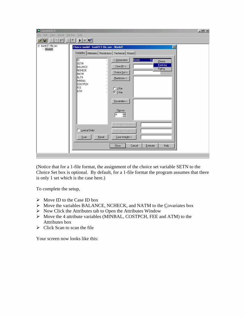
(Notice that for a 1-file format, the assignment of the choice set variable SETN to theChoice Set box is optional. By default, for a 1-file format the program assumes that thereis only 1 set which is the case here.)

To complete the setup,

Ø Move ID to the Case ID boxØ Move the variables BALANCE, NCHECK, and NATM to the Covariates boxØ Now Click the Attributes tab to Open the Attributes WindowØ Move the 4 attribute variables (MINBAL, COSTPCH, FEE and ATM) to the

Attributes boxØ Click Scan to scan the file

Your screen now looks like this:

Notice that by default the attribute ATM is treated as ‘Nominal’ while the others aretreated as ‘Numeric’. That is because in the SPSS .sav file, ATM is defined as a string(character) variable, while the others take on the equidistant numeric values used byKamakura et. al.

To view the numeric values assigned to these attributes, you may open the Score box.

Ø Double click on MINBAL to open the score box for this numeric attribute

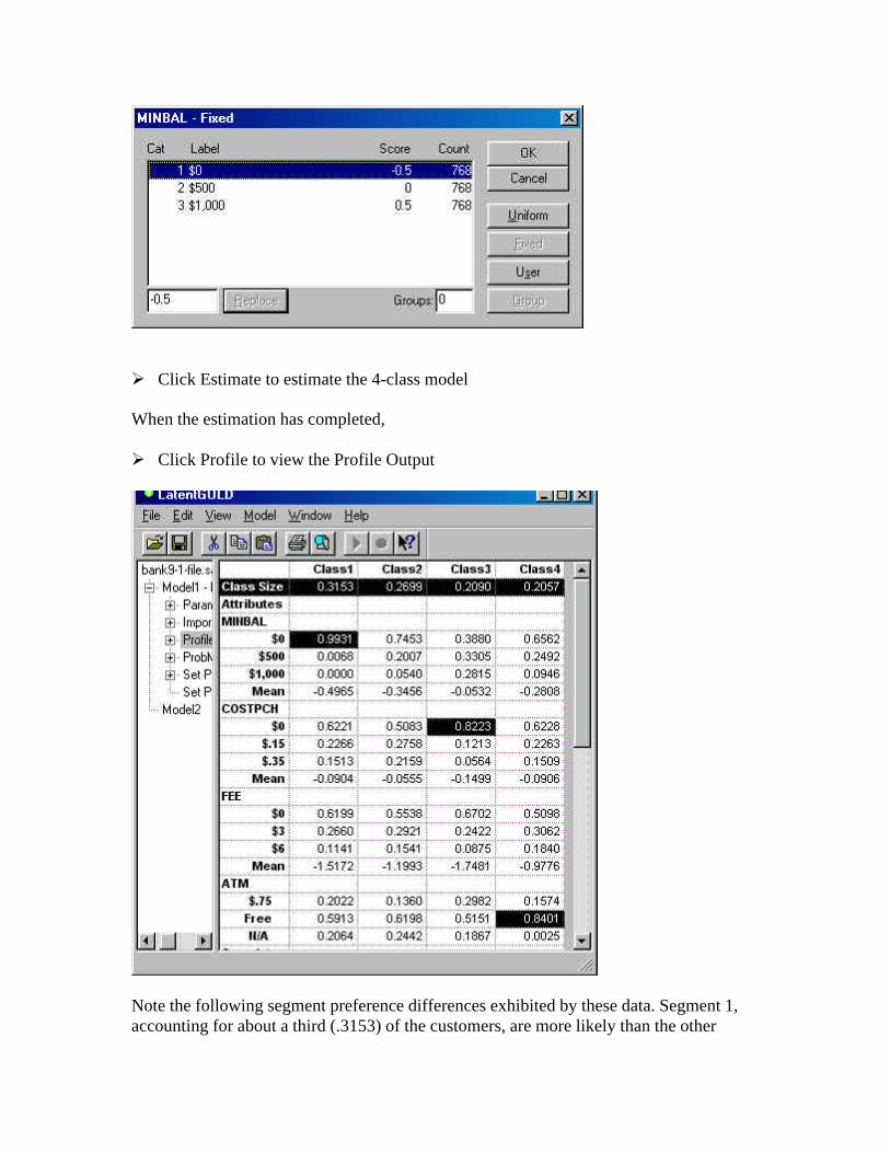
Ø Click Estimate to estimate the 4-class model

When the estimation has completed,

Ø Click Profile to view the Profile Output

Note the following segment preference differences exhibited by these data. Segment 1,accounting for about a third (.3153) of the customers, are more likely than the other

segments to prefer alternatives offering a ‘No minimum balance’ option (the re-scaledpart-worth utility associated with MINBAL = $0 is .9931). Segment 3, accounting forabout 21% of the customers) gives more weight to no check-writing cost (re-scaledparameter associated with COSTPCH = $0 is .8223). In contrast, Segment 4, accountingfor 21% of the customers, is more influenced by free ATM availability (ATM = ‘Free’).The preferences for Segment 2, accounting for the remaining 27% of customers, fallssomewhere between these other segments in their preferences.

Ø Scroll down to display the covariate distributions

Latent GOLD Choice provides the segment means for each covariate as well as segmentdistributions associated with 5 grouped levels (from low to high) of these variables.Notice that segment 1, the segment having the highest utility for ‘no minimum balance’requirement, maintains a much lower balance than the other segments (a mean of $577.71compared to $1,138.96 for segment 4 and higher for the other segments). Segment 4, thesegment with the highest utility for free ATM use, has utilized ATMs more than the othersegments. Similarly, segment 3, the segment most influenced by the ‘no cost per check’option, writes more checks than the others.

These differential preferences can be seen even more clearly by examining theImportance output

Ø Click on Importance to display the Importance Output file

Ø Click on expand icon (+) to the left of ImportanceØ Click on Imp-Plot to display the Importance PlotØ Click on ‘Class1’ below the plot to view graphically how segment 1 differs from the

other segments in Importance

See Kamakura et. al. for similar interpretations of these segments. The numbering ofthese segments differs from the article because Latent Gold Choice assigns segmentnumbers by segment size. The correspondence between Latent Gold Choice segmentsand segments described in the Kamakura et. al. article is:

Latent GOLD Choice à Kamakura et. al.1 à 42 à 33 à 14 à 2

We will now examine some further graphical output.

For each segment, the Set Profile Output presents the predicted probability of the highestranked alternative. To display these probabilities graphically,

Ø Click on expand icon (+) to the left of Set ProfileØ Click on Prf-Plot to display the Set Profile PlotØ Click on Class3 at the bottom of the plot

Notice that segment 3 is much more likely to rank alt#7 highest (the predicted probabilityfor doing this is .43) than the other segments. The corresponding probability is less than.05 for each of the other segments.

Ø Click on expand icon (+) to the left of ProbMeansØ Click on Tri-Plot which contrasts 3 groups of segments

By default, the tri-plot contrasts segment 1, segment 2, and the combined segments 3 and4. Since segments 3 and 4 are very different, it would be more informative to groupsegments 1 and 2. To customize the tri-plot so that the upper vertex corresponds tosegments 1 and 2,

Ø Right-click on the tri-plot to retrieve the Plot control

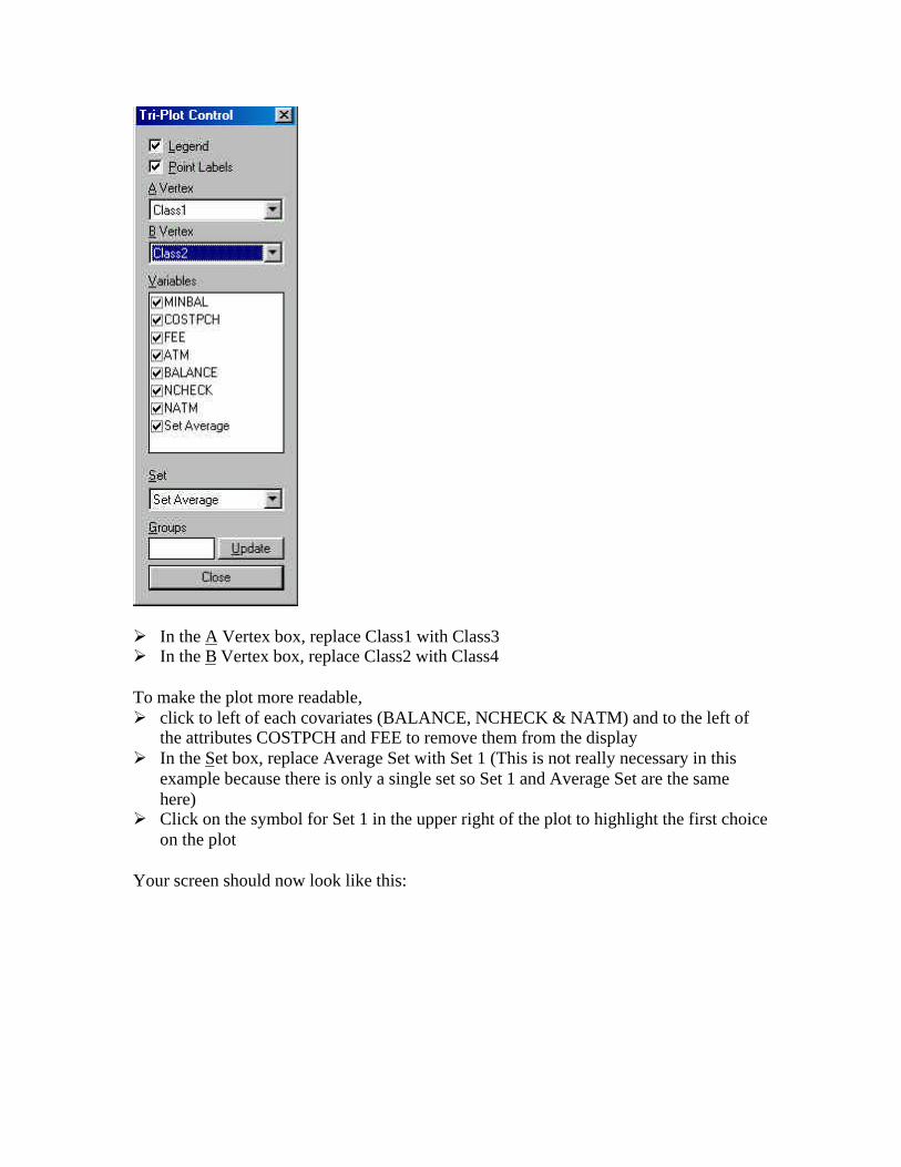
Ø In the A Vertex box, replace Class1 with Class3Ø In the B Vertex box, replace Class2 with Class4

To make the plot more readable,Ø click to left of each covariates (BALANCE, NCHECK & NATM) and to the left of

the attributes COSTPCH and FEE to remove them from the displayØ In the Set box, replace Average Set with Set 1 (This is not really necessary in this

example because there is only a single set so Set 1 and Average Set are the samehere)

Ø Click on the symbol for Set 1 in the upper right of the plot to highlight the first choiceon the plot

Your screen should now look like this:

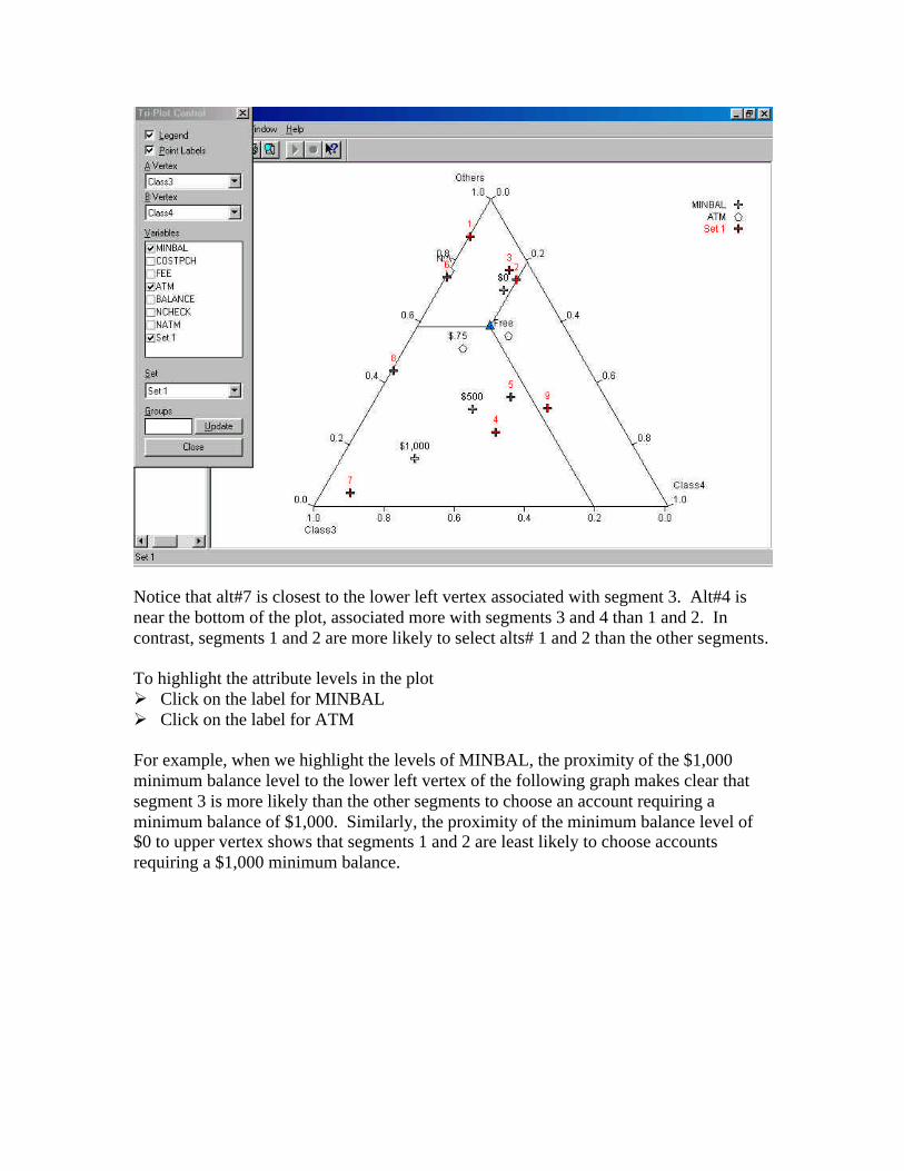
Notice that alt#7 is closest to the lower left vertex associated with segment 3. Alt#4 isnear the bottom of the plot, associated more with segments 3 and 4 than 1 and 2. Incontrast, segments 1 and 2 are more likely to select alts# 1 and 2 than the other segments.

To highlight the attribute levels in the plotØ Click on the label for MINBALØ Click on the label for ATM

For example, when we highlight the levels of MINBAL, the proximity of the $1,000minimum balance level to the lower left vertex of the following graph makes clear thatsegment 3 is more likely than the other segments to choose an account requiring aminimum balance of $1,000. Similarly, the proximity of the minimum balance level of$0 to upper vertex shows that segments 1 and 2 are least likely to choose accountsrequiring a $1,000 minimum balance.

Classification output

Let's now turn to classifying respondents into the appropriate segments. For eachrespondent, the classification tables show the posterior membership probabilityassociated with each class as well as the segment, along with the segment for which thisprobability is highest (displayed in the column marked ‘Modal’). The standardclassification output takes into account responses as well as covariate information, whilethe covariate classification output uses only covariate information to compute theseprobabilities.

To view the standard classification output,

Ø On the left-hand screen, click on Model1Ø Click on Output to open the output tab in the Model Analysis Dialog BoxØ Click on Classification Information to request this outputØ Click Estimate to re-estimate the model

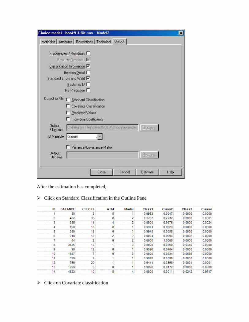
After the estimation has completed,

Ø Click on Standard Classification in the Outline Pane

Ø Click on Covariate classification

Now we will examine how well the model predicts the alternative that is ranked highest

Ø Click on Model 1Ø Scroll down to display the prediction table

Notice that except for the 2 respondents who made other choices, the numbers in theright-most ‘Total’ column show that only 4 of the 9 alternatives were ranked highest.Specifically, we see that alt#1 was ranked highest by n=9 respondents, alt#2 by n=139),alt#4 by n=58 and alt#7 by the remaining 28. In our next tutorial, we will show how wecan exploit this fact in model estimation .

Ø Now, scroll up to the Prediction Statistics

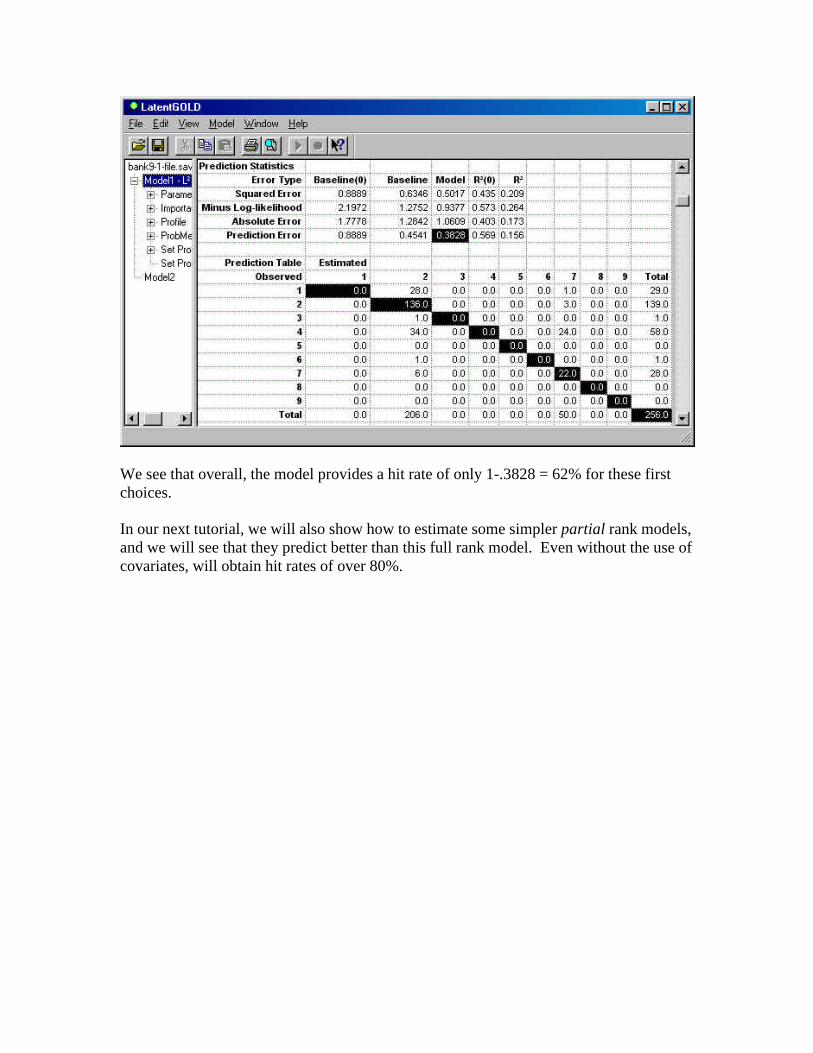
We see that overall, the model provides a hit rate of only 1-.3828 = 62% for these firstchoices.

In our next tutorial, we will also show how to estimate some simpler partial rank models,and we will see that they predict better than this full rank model. Even without the use ofcovariates, will obtain hit rates of over 80%.

References

Kamakura, W., Wedel, M., Agrawal, J. 1994. Concomitant variable latent class modelsfor conjoint analysis. International Journal of Research in Marketing 11, 451-464.