Two-Settlement Electric Power Marketswith Dynamic-Price Contracts

27 July 2011

IEEE PES GM, Detroit, MI

Last Revised: 24 July 2011

1

Huan Zhao, Auswin Thomas, Pedram Jahangiri,Chengrui Cai, Leigh Tesfatsion, and Dionysios Aliprantis

Presentation Outline• Overview of Integrated Retail/Wholesale (IRW) project at Iowa State University

• Two Dynamic‐Pricing Studies:– First Study:  Effects of price‐responsive retail consumer demand on LSE demand bidding and profit outcomes, both with and without LSE learning. 

– Second Study:  Determination of a household resident’s optimal comfort‐cost trade‐offs by a smart HVAC system conditional on contract terms, prices, outdoor temperature, and other forcing terms  

• Conclusion

Project Directors: Leigh Tesfatsion (Professor of Econ, Math, & ECpE, ISU) Dionysios Aliprantis (Assistant Prof. of ECpE, ISU) David Chassin (Staff Scientist, PNNL/Department of Energy) Research Assoc’s: Dr. Junjie Sun (Fin. Econ, OCC, U.S. Treasury, Wash, D.C.) Dr. Hongyan Li (Consulting Eng., ABB Inc., Raleigh, NC) Research Assistants: Huan Zhao (Econ PhD student, ISU)

Chengrui Cai (ECpE PhD student, ISU)

Pedram Jahangiri (ECpE PhD student, ISU)

Auswin Thomas (ECpE M.S. student, ISU)

Di Wu (ECpE PhD student, ISU)

Current Government & Industry Funding Support: PNNL/DOE, the Electric Power Research Center (an industrial consortium), and the National Science Foundation Industry Advisors: Personnel from PNNL/DOE, XM, RTE, MEC, & MISO

IRW Project:IRW Project: Integrated Retail/Wholesale Power Integrated Retail/Wholesale Power System Operation with SmartSystem Operation with Smart--Grid FunctionalityGrid Functionality

4

Meaning of “Smart Grid Functionality”?

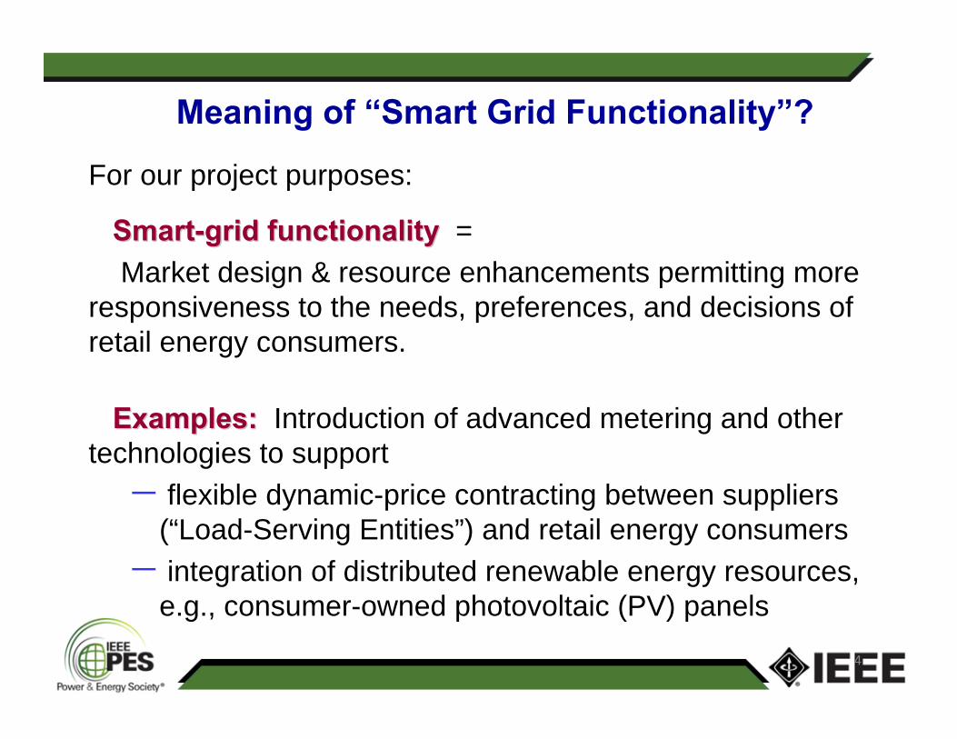
For our project purposes:

SmartSmart--grid functionalitygrid functionality = Market design & resource enhancements permitting more

responsiveness to the needs, preferences, and decisions of retail energy consumers.

Examples:Examples: Introduction of advanced metering and other technologies to support − flexible dynamic-price contracting between suppliers

(“Load-Serving Entities”) and retail energy consumers − integration of distributed renewable energy resources,

e.g., consumer-owned photovoltaic (PV) panels

5

Principal IRW Project Research Topics

Dynamic retail/wholesale reliability and efficiency implications of integrating demand response resources as realized thru

Top-down demand response (e.g., emergency curtailment) Automated demand dispatch (continuous signaling)Price-sensitive demand bidding by demand resources

Dynamic retail/wholesale effects of increased penetration of consumer-owned distributed energy resources, such as photovoltaic (PV) generation & plug-in electric vehicles (PEV)

Development of agent-based algorithms for smart device implementation (e.g., “smart” HVAC systems)

6

Primary Project Tool:The IRW Power System Test Bed

An agent-based computational laboratory“Culture dish” approach to complex dynamic systemsPermits systematic computational experiments Permits sensitivity testing for changes in physical constraints (e.g., grid configuration), market rules of operation, and participant behavioral dispositions

Seams empirically grounded test beds (AMES/GridLAB-D)Market rules based on business practices manuals for restructured North American electric power markets

Realistically rendered transmission/distribution networksRetail contracting designs based on case studies (e.g., ERCOT) and pilot studies (e.g., Olympic Peninsula 2007)

Open source software release planned.

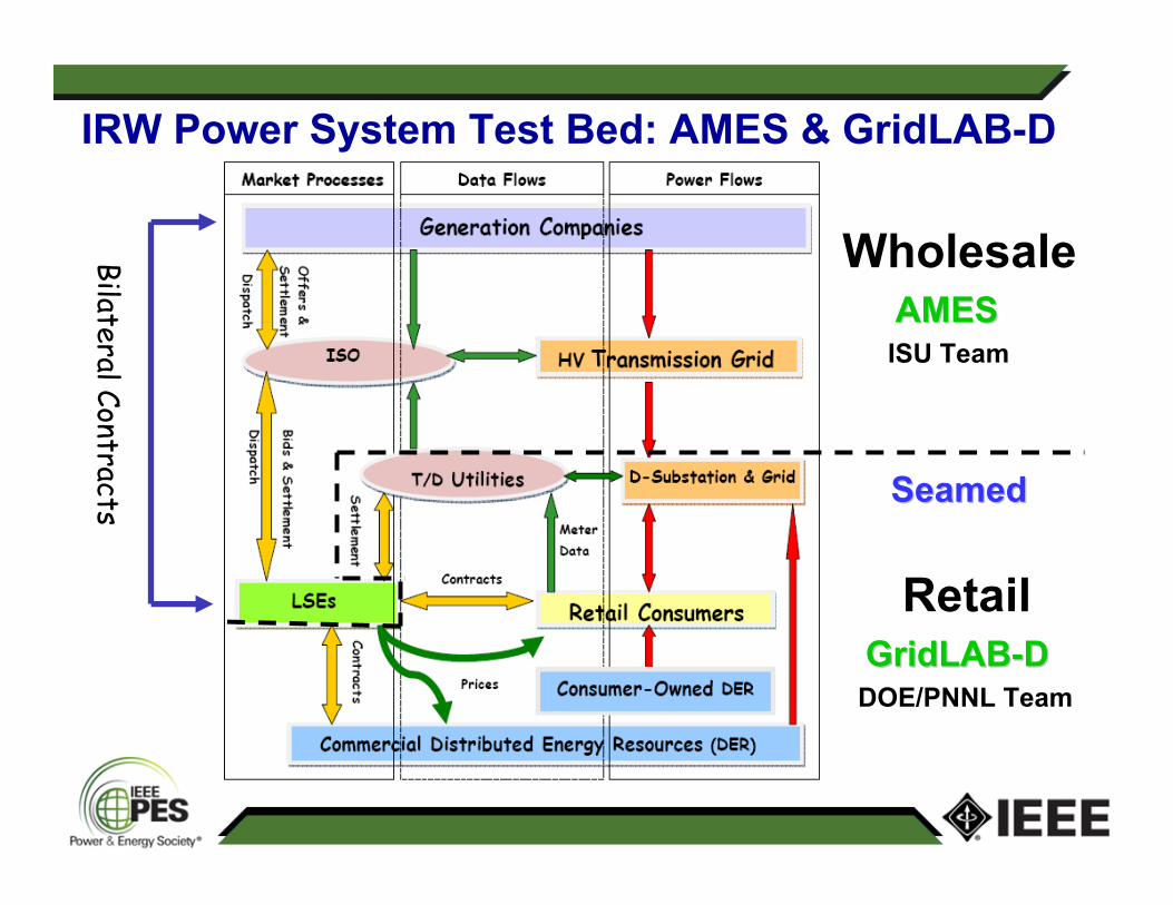
WholesaleAMES AMES

ISU Team

RetailGridLABGridLAB--D D

DOE/PNNL Team

Seamed Seamed

x

x

Bilateral Contracts

IRW Power System Test Bed: AMES & GridLAB-D

Seams AMES (wholesale) & GridLAB-D (retail) with a retail focus on households with price-sensitive loads

IRW Power System Test Bed (Version 1.0)

Typical Day-D Market Operator (ISO) Activities

First Study: LSEs Servicing Residential HVAC Loads

10

Five-Bus Grid Configuration with Three LSEs

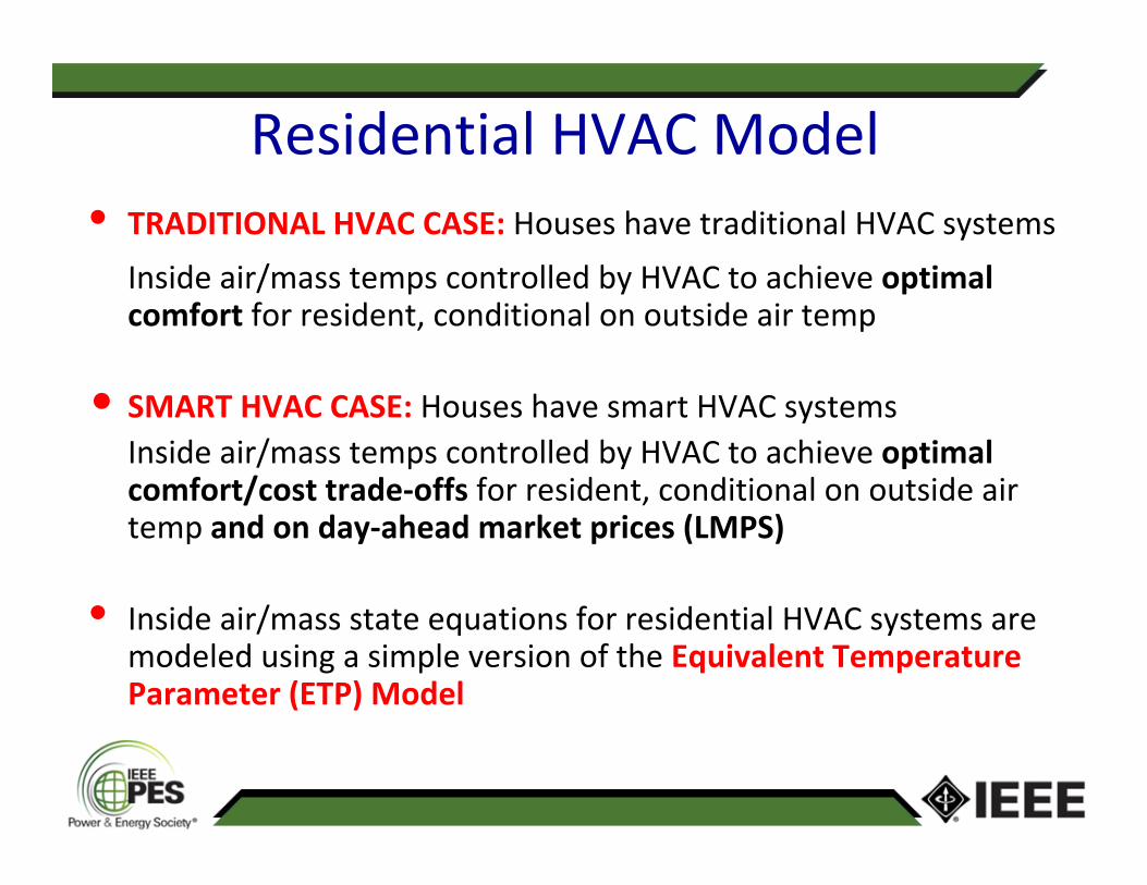
Residential HVAC Model• TRADITIONAL HVAC CASE: Houses have traditional HVAC systems

Inside air/mass temps controlled by HVAC to achieve optimal comfort for resident, conditional on outside air temp

• SMART HVAC CASE: Houses have smart HVAC systems Inside air/mass temps controlled by HVAC to achieve optimalcomfort/cost trade‐offs for resident, conditional on outside air temp and on day‐ahead market prices (LMPS) 

• Inside air/mass state equations for residential HVAC systems aremodeled using a simple version of the Equivalent Temperature Parameter (ETP) Model

Benchmark Outcomes:LMP and Fixed Load Profiles for Traditional HVAC Case

12

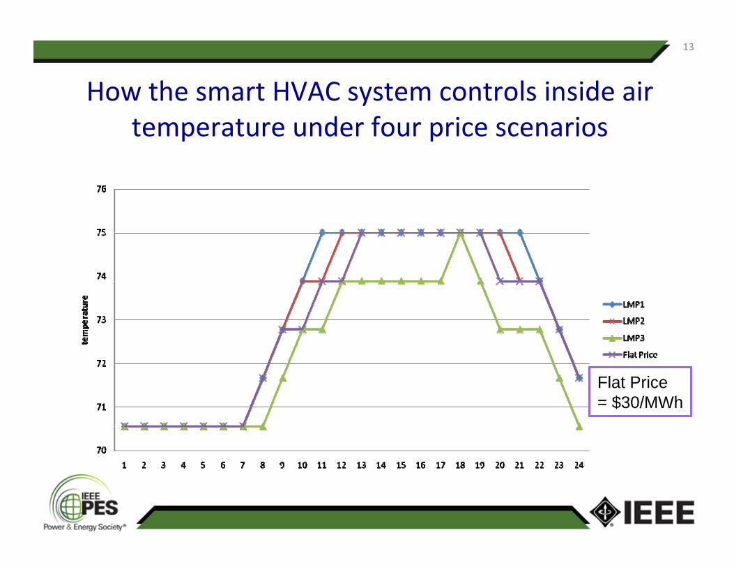
How the smart HVAC system controls inside air temperature under four price scenarios

13

Flat Price= $30/MWh

Household Energy Consumption for Traditional HVAC Case and for Smart HVAC Case (four price scenarios)

14

Traditional HVAC(no price response)

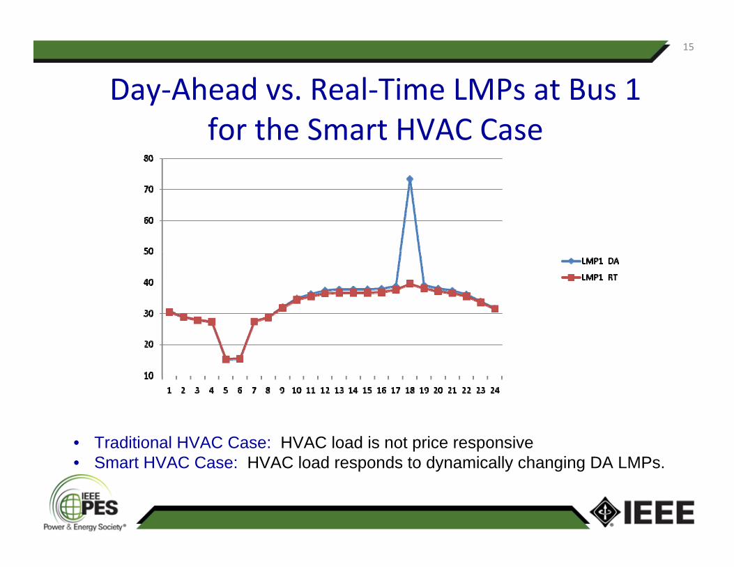
Day‐Ahead vs. Real‐Time LMPs at Bus 1 for the Smart HVAC Case

• Traditional HVAC Case: HVAC load is not price responsive• Smart HVAC Case: HVAC load responds to dynamically changing DA LMPs.

15

LSE Profits are Negative for Smart HVAC Case

( , ) 0corr P QΔ Δ >

16

Market Robustness

• Key Issues:

– Does changing from the traditional HVAC case (fixed load) to smart HVAC case (price‐responsive load) result in 

• peak load shift?

• discrepancies between day‐ahead and real‐time prices?

– How does this change affect the demand bidding behavior of the LSEs in the DA market?

17

Market Robustness TestFlow Diagram

18

Penetration of Smart HVAC

System WithoutSmart HVAC

LSE Chooses Bidding Curve

One Learning Cycle

LSE Updates Belief of Bidding Action

Max Iteration Reached?

Weather StateRevealed

Analyze SimulationResult

No Yes

Learning Experiments forthe Three LSEs

19

Outdoor temperatures differ across the bus locations of the three LSEs

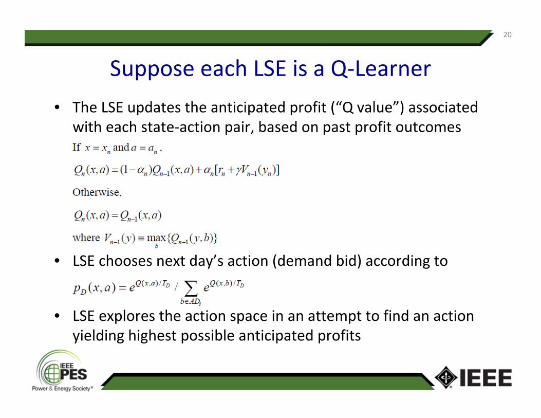
Suppose each LSE is a Q‐Learner 

• The LSE updates the anticipated profit (“Q value”) associated with each state‐action pair, based on past profit outcomes

• LSE chooses next day’s action (demand bid) according to 

• LSE explores the action space in an attempt to find an action yielding highest possible anticipated profits 

20

Simulation Results (100 Days)Daily Average Profits for the Three Learning LSEs

21

DAY0 100

Simulation Results (100 Days)…ContinuedHourly Average Load Deviations for the Three Learning LSEs

22

DAY0 100

Simulation Results…ContinuedMarket Performance Comparison

23

• On day D=1, smart HVAC replaces traditional HVAC. LSEs do not have enough information to estimate smart HVAC price responsiveness

• During next 100 days, LSEs use learning to adjust their DA market demand bids in an attempt to maximize their profits

• By day D=100, the LSEs have learned how to make DA market demand bids that more properly account for smart HVAC price responsiveness.

Market Robustness Findings• Over time the LSEs learn how to adjust to smart HVAC demand response and select their DA market demand bids to maximize their profits.

• By day 100, LSE demand bids appear to have stabilized.

• By day 100, the DA and RT markets have evolved to a coordinated outcome where the prices in the two markets are essentially the same.

24

Second Study:Controller Design for Smart HVAC System

26

Modeling of a Smart HVAC System (HVAC = Heating-Ventilation-Air-Conditioning)

• Inputs include:Preferences of a household resident trying to achieve optimal daily trade-offs between comfort and costs Structural home attributes (e.g., square footage & insulation level)Electricity prices (e.g. fixed regulated price, market-based LMPs)Forcing terms (outdoor temp, solar radiation, control actions)State equations for a two-dimensional state vector x(t) consisting of (1) Indoor air temp Ta(t) and (2) indoor mass temp Tm(t) , e.g. for furniture and walls.

27

ETP Modeling of HVAC State Equations

• The house resident has a “bliss” temp (e.g., 72oF)

• Using a discretized form of ETP state equations, HVAC sets its status levels (from cooling to heating) to achieve optimal comfort/cost trade-offs for the resident over time, conditional on forecasted prices, outdoor temp, & other forcing terms.

• HVAC status levels derived via dynamic closed-loop control.

External and Internal Forcing Terms

28

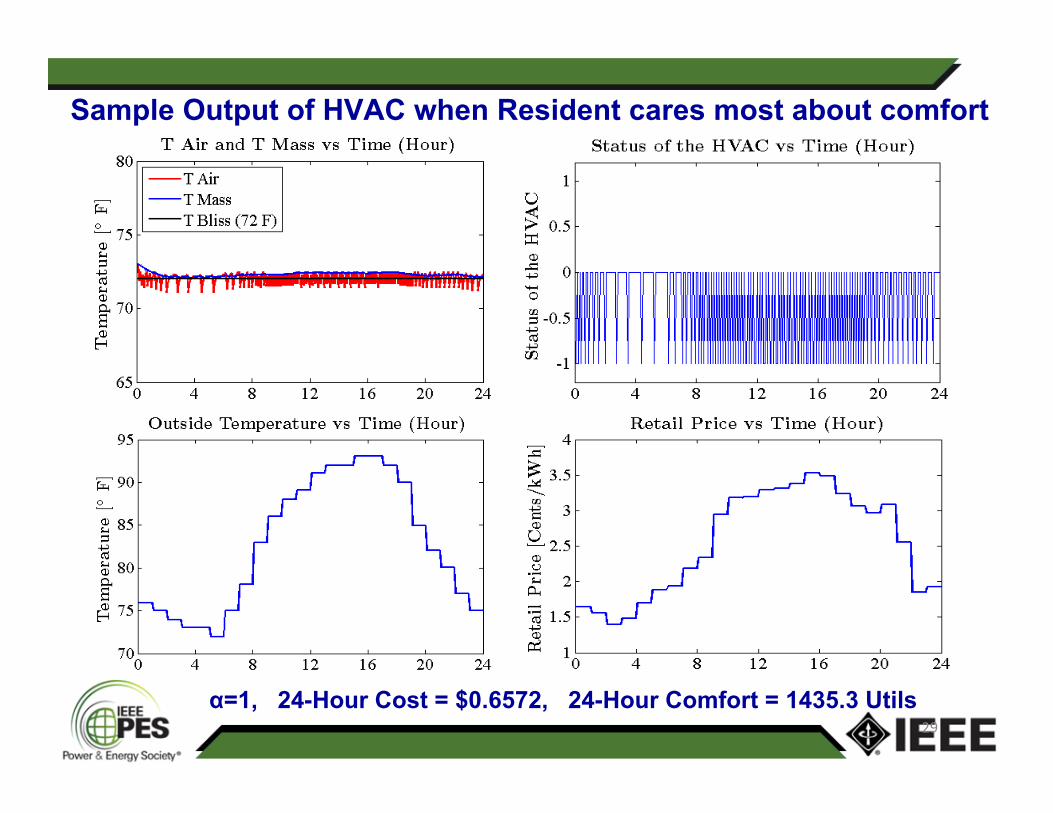
Sample Output of HVAC when Resident cares most about comfort

29

α=1, 24-Hour Cost = $0.6572, 24-Hour Comfort = 1435.3 Utils

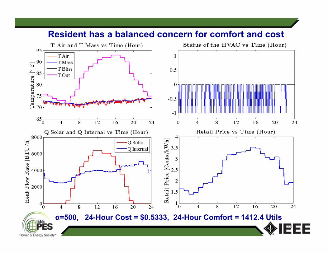
Resident has a balanced concern for comfort and cost

30

α=500, 24-Hour Cost = $0.5333, 24-Hour Comfort = 1412.4 Utils

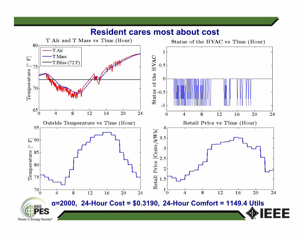
Resident cares most about cost

31

α=2000, 24-Hour Cost = $0.3190, 24-Hour Comfort = 1149.4 Utils

Sample Output of HVAC when Resident cares most about comfort

32

α=1, 24-Hour Cost = $0.6572, 24-Hour Comfort = 1435.3 Utils

Resident has a balanced concern for comfort and cost

33

α=500, 24-Hour Cost = $0.5333, 24-Hour Comfort = 1412.4 Utils

Resident cares most about cost

34

α=2000, 24-Hour Cost = $0.3190, 24-Hour Comfort = 1149.4 Utils

Variation of Cost and Comfort with Alpha(Low Alpha → Stress On Comfort, High Alpha → Stress on Cost)

35

36

Dynamic Pricing Studies: Summary and Future Planned Work

Impact of retail consumer price-responsive demand on LSE demand bidding and LSE profit outcomes, both with and without LSE learning.

Design of a smart residential HVAC controller to achieve optimal comfort-cost trade-offs conditional on prices and forcing terms (e.g., outdoor temp)

Goal: Use IRW Test Bed to study carefully the effects of various types of Demand Response (DR) on retail and wholesale power system operations