types of images - carnegie mellon university// ... mechanism of that attenuation is ionization of...

42-101 Intro to BME (Spring 2005) 10.1 Topic 10. Biomedical Imaging Topics

- Biomedical imaging overview - Magnetic Resonance Imaging - Handling and Processing Image Data, the Fourier transform

Biomedical Imaging Overview Types of Images http://www-ipg.umds.ac.uk/mpss99/Lecture_Notes/intro_html/imaging_intro.html

Medical images come in a wide variety of forms: much more than the standard still and moving pictures produced with optical cameras. Medical images can take the form of projections, slices or volumes.

Projections

Many medical images are a projection of the three dimensional (3D) patient onto a two dimensional (2D) plane. Projections can be orthogonal or perspective. Considering object coordinates to be defined using (x,y,z),and image coordinates as (u,v), the projections can be drawn as:

42-101 Intro to BME (Spring 2005) 10.2 Topic 10. Biomedical Imaging Slices/Tomographs

Most medical images that are not projections, are made up of one or more slices. The orientation of the slices are defined anatomically:

• transaxial - plane normal to a vector from head to toe. • coronal - plane normal to a vector from front to back • sagittal - plane normal to a vector from left to right. • oblique - a slice that is not (at least approximately) one of the above.

A medical image might be made of • a single slice • a series of parallel slices with uniform spacing • a series of slices with varying spacing and/or orientation

• Volumes • In some types of medical image, data is acquired from an entire volume

in one go (note this is different from acquiring multiple slices, one after the other).

Dimensionality

In medical imaging, the subject being imaged has three spatial dimensions, and changes with time. The dimensionality of the images is, however, variable.

• Two spatial dimensions - eg: standard x-ray, single ultrasound image • Three spatial dimensions - multiple slices or volume acquisition. • Time dimension -In many cases, it take time to acquire information about

the object, so for many images with 2D or 3D spatial information, it is assumed that the patient is still - if they move the image gets degraded by artefact. Other times, it is desirable to image dynamic change eg: ultrasound of beating heart

• Higher dimensionality eg: scale space, different modalities • One dimensional: a single line representing a projection through all or part

of the subject.

42-101 Intro to BME (Spring 2005) 10.3 Topic 10. Biomedical Imaging

http://info.med.yale.edu/intmed/cardio/imaging/techniques/project_vs_tomographic/index.html Because of the nature of trans-illumination ("shadowgram-like" illumination) in projection techniques, various tissues are imaged as overlapping each other and often need multiple views (thus the PA and Lateral) for visual understanding.

Tomographic images are thin slices (and can be generated by x-rays in the case of computed tomography, or ultrasound in the case of echocardiography) and allow presentation of anatomy in a more readily understandable way because they avoid the confusion of overlapping structures.

42-101 Intro to BME (Spring 2005) 10.4 Topic 10. Biomedical Imaging Ionizing versus Non-ionizing radiation imaging techniques info.med.yale.edu/intmed/cardio/imaging Medical imaging techniques can be broadly grouped into those which use ionizing radiation versus those that do not. The ionizing radiation group consists of those images created by the use of x-rays or gamma rays. Both x-rays and gamma rays are high energy, short wavelength (less than an angstrom) electromagnetic radiation that is capable of penetrating and passing through most tissues. Gamma rays arise from the nuclear decays of radioactive tracers introduced into the body, while x-rays arise from an x-ray tube where high speed electrons bombard a small spot on a tungsten anode target.

Ionizing radiation, as it passes through the body is differentially absorbed by tissues of greater thickness or higher atomic mass (e.g. calcium has a higher atomic weight than hydrogen which is a major component of tissue water). Different portions of the body tissues attenuate differing amounts of the incident radiation. One mechanism of that attenuation is ionization of the tissue atoms which make them chemically reactive and potentially capable of cell damage. Ionizing radiation is therefore not used casually but only when medically indicated. X-rays are nonetheless highly useful diagnostically and are a backbone of medical imaging by both computed tomography and film. It is the locally differential pattern of x-ray radiation escaping the body that creates the "shadowgram" on an x-ray film. That escaping radiation strikes a fluorescent screen inside a film cassette, and fluorescent light from those screens in turn expose the film emulsion (n.b.: if x-ray film was actually only sensitive to exposure by x-rays, we wouldn't need darkrooms for handling those films).

Non-ionizing radiation techniques mainly use either acoustic pulses (ultrasound) for echo-ranging imaging (somewhat like radar) or radio-waves combined with high-field magnets, in the case of magnetic resonance imaging.

http://info.med.yale.edu/intmed/cardio/imaging/techniques/ionizing_vs_nonionizing/index.html

42-101 Intro to BME (Spring 2005) 10.5 Topic 10. Biomedical Imaging Energy Content of Radiation

http://info.med.yale.edu/intmed/cardio/imaging/techniques/em_spectrum/index.html

E = hν h = Planck’s constant, 6.626×10-34 J•s = 6.626×10-27 erg•s ν = frequency of radiation in Hz (1/s)

note that λ = c/n where λ is the wavelength of radiation and c is the speed of light (299,792.458 m/s)

42-101 Intro to BME (Spring 2005) 10.6 Topic 10. Biomedical Imaging Ionizing radiation Ionizing radiation is a portion of the high energy electromagnetic radiation spectrum which can penetrate and be transmitted through tissues (unlike light, which is mostly absorbed at the skin surface, failing to adequately penetrate thick body parts such as the skull). One of the chief modes by which ionizing radiation interacts with tissues is by knocking out atomic shell electrons, losing energy in the process. The resulting differential absorption can be detected by a film cassette at the opposite side of the body from the radiation entrance. It is this differential absorption that permits a "shadowgram of the body" (i.e. an "Xray film") to be created which differently displays bones and soft tissues of various thicknesses as patterns of light and darkness.

This Ionizing radiation is high energy (short wavelength - e.g. 0.1 to 0.001 angstrom range) electromagnetic waves. These radiation waves are created either by radioactive nuclear decay of tracer atoms injected into the body (nuclear medicine) or by Xray tubes (which create their energy waves by bombarding a tungsten anode target with high energy [40 to 150 keV] electrons). Transducing these waves into light by a fluorescent screen, sodium iodide crystal, or by photon counters allows images (say, of differential tissue absorption - or of the radioactive atomic locations in the case of nuclear tracers) to be formed into an image on film or displayed on a cathode ray tube display.

http://info.med.yale.edu/intmed/cardio/imaging/techniques/ionizing_radiation/index.html


Radiography – a projection technique that uses ionizing radiation X-ray technology X-ray imaging is a method of illuminating the body with a penetrating high energy ionizing radiation. The differential absorption of this radiation by the various tissues of the body creates on film an inverse shadow of the body. Less dense, lower atomic weight structures, such as the lung, allow transmission of more radiation flux producing greater fluorescence on an absorbing screen which exposes an adjacent film more densely, making those areas black. Higher atomic weight structures (bone) absorb and block the radiation and thus do not result in the exposure of the silver halide grains in the film emulsion, and so bony structures such as the ribs appear white (transparent).

The heart, as a large, mainly water-like density, absorbs much of the incident radiation, so it looks light on the film. The main limitation of X-ray imaging is that because it is a projection technique, body structures overlap one another and thus often at least two views (e.g. PA and lateral) are required. Moreover, when many water density organs lie on top of each, such as in the abdomen, they absorb radiation to a similar degree and thus lack sufficient contrast density to be discriminable on the film even with multiple views. Notice that on an X-ray of the chest, the main features are the heart, bony structures, and fine vessel structures in lung. An x-ray of the abdomen provides little features other than bony spine and pelvis and gas in the bowel.

http://info.med.yale.edu/intmed/cardio/imaging/techniques/forming_rad_images/index.html

42-101 Intro to BME (Spring 2005) 10.8 Topic 10. Biomedical Imaging Radiographic density As Ionizing radiation passes through the body, it is differentially absorbed by tissues of greater thickness or high atomic mass (e.g. calcium). Different portions of the body tissues attenuate differing amounts of the incident radiation. The radiographic density is mainly the result of x-ray radiation scattering or loss of the incident radiant energy by ionization. It is the locally different amount of x-ray radiation escaping from the body that creates the resulting "shadowgram" on an x-ray film, by striking a fluorescent screen, which in turn exposes the film emulsion (if x-ray film was actually only sensitive to exposure by x-rays, we wouldn't need darkrooms for handling the films). The range of densities that an X ray can display is the key to its usefulness as a diagnostic imaging tool. The X ray tube emits a large burst of X rays, generated by bombarding a tungsten target in a vacuum tube with high energy electrons (40 to 150 keV). Many of these X rays when directed toward a person will pass through the body and strike a fluorescent screen in a cassette, exposing a light-sensitive film adjacent to it (n.b.: "X ray film" is not really X ray sensitive, but is rather is a light sensitive film exposed by light photons emitted from X ray sensitive fluorescent screens in close contact with it). One concept frequently hard to understand is that the "white", or transparent part of an X ray film lies behind tissues that block or absorb most of the X rays entering the body in that area such as bone or thick body parts. X ray absorption is dependent on both the thickness (path length) of tissue that it must traverse and/or the atomic weight of body materials. High atomic weight tissues (bone, metal implants) or long path lengths (liver, excessive fat) absorb or scatter the X rays before they can exit the body resulting in unexposed, or transparent parts on the film. The darker, blacker parts of the film lie behind thin tissues or low density tissue (lung) that allows much of the X ray beam (a high flux of radiation) to traverse it without absorption.

http://info.med.yale.edu/intmed/cardio/imaging/techniques/radiographic_density/index.html

42-101 Intro to BME (Spring 2005) 10.9 Topic 10. Biomedical Imaging X-ray imaging example – position of a pacemaker The PA (postero-anterior) radiograph at first appears to provide reassuring evidence that the tip of the pacemaker lies in the right ventricular apex. The slightly thickened metal tip of the pacemaker is seen just lateral to the border of the descending aorta near the diaphragm. The value of a lateral radiograph is best exemplified (click the "Lateral X-ray"button located on the right side of the main screen) when the course of the pacemaker wire is followed inferior and is found to lie well posterior to the expected position of the right ventricular cavity. The only course which this wire can occupy is if the tip of the catheter lies within the coronary sinus which is entered in the right atrium just proximal to the tricuspid valve and is the major draining coronary vein in the atrio-ventricular groove emptying into the lower right atrium. The pacer wire would have to be withdrawn and placed properly at the right ventricular apex.

http://info.med.yale.edu/intmed/cardio/imaging/findings/value_of_lateral/index.html


Angiography – a projection technique that uses ionizing radiation Similar to the x-ray technique – a radiopaque (x-ray adsorbing) dye, is injected into the circulatory system to provide contrast with the surroundking soft tissue. Coronary angiography requires multiple separate views to completely examine coronary anatomy and resolve potential vessel overlap. Several separate sequential injections of left (LCA) and right coronary arteries (RCA) are shown. Here, "postero - anterior" (PA), "left anterior oblique" (LAO), and "right anterior oblique" (RAO) views of a normal coronary tree are provided. The "Left Ventriculogram" is an RAO view with direct contrast injection into the cavity to examine myocardial function.

http://info.med.yale.edu/intmed/cardio/imaging/techniques/angiography/index.html


Endoscopy – a projection/refraction technique that uses non-ionizing radiation An endoscope is essentially an elaborate flashlight – visible light is passed through a fiber optic bundle to illuminate a tissue remotely and the image is viewed through a second, coaxial fiber. Tissues are largely opaque to visible light, although red/infrared light may penetrate tissues to a significant extent.

An example of a laproscopic endoscope… http://www.endoscopy.md/laparoscopy.html

IEC-Innovative Endoscopy Components, LLC is a manufacturer of high quality Rigid Endoscopes such as our Laparoscope "Made in Germany". All our Rigid Endoscopes like the Arthroscope, Cystoscope, Hysteroscope, Otoscope, Sinuscope, Laryngoscope and Bronchocope are manufactured according to ISO 9001 standards, featuring the most excellent design elements for today's Surgical Equipment Industry.

picture 08: Laparoscope Ø 10 mm, 30°, l=310 mm

42-101 Intro to BME (Spring 2005) 10.12 Topic 10. Biomedical Imaging Example endoscope images. http://www.gicare.com/pated/eiegnmeg.htm

The Larynx This is what your voice box looks like from above. You notice the vocal cords on each side. These move back and forth as air is forced out over the cords. Amazingly, these simple fibrous bands of tissue allow us to talk, whisper, shout and sing the entire range of melodious and rich bass tones. This is a normal appearance of the larynx.

Esophagus This picture is an image of the middle of the esophagus. It has a wide open tubular appearance and pink coloration. Seconds after this picture was taken, a contraction occurred. These normal sweeping wavelike contractions are what move food and liquid from the mouth to the stomach.

Lower Esophageal Sphincter These are images of the end of the esophagus. There is a specialized muscle here which acts like a valve and which is called the lower esophageal sphincter (LES). It remains closed most of the time, only opening to allow swallowed food and liquid to be swept through into the stomach. When you belch, the air pressure in the stomach overcomes the pressure of the valve and the air you have swallowed bursts up the esophagus past this valve. The LES in the left image is closed while that in the right image is open.


Computed Tomograpy – a tomographic technique that uses ionizing radiation

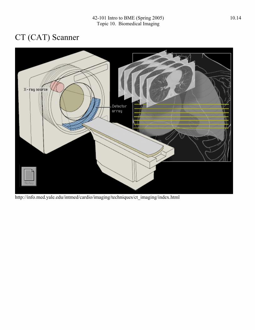
Computed tomography is a digitally based x-ray technique. Like x-ray, the resulting images arise from differential x-ray absorption of tissue, a feature that rests primarily on atomic weight (and thus the electron density) of the various tissues. The technique uses a narrowly collimated x-ray beam to irradiate a slice of the body. The amount of radiation transmitted along each projection line is collected by photo-multiplier tubes and counted digitally. By rapidly acquiring views from numerous different projections, achieved by quickly rotating the tube and detectors around the body, the transmissivity of the body from different angles can be established externally.

Once these transmission values are collected, they can be digitally filtered and back-projected mathematically (by a technique known as Fourier transformation) onto a matrix which represents fine differentiation of tissue densities. Mapping this density onto what is called the Hounsfield scale where bone is +1000 and air is -1000, resolves as subtle as 1/2 a percent electron density within half millimeter volumes of tissue. This distinction is enough to discriminate most of the soft tissue organs of the brain and abdomen, not to mention the lungs and mediastinum. Since the image is digital and represents a slice, multiple slices can be obtained and a volume estimated and displayed as a three-dimensional structure on a video display tube or film. Computed tomography has the advantage of rapid acquisition of images, but employs ionizing x-ray radiation which must be used conservatively to avoid harmful cumulative biologic effect.

http://info.med.yale.edu/intmed/cardio/imaging/techniques/tomography/index.html


CT (CAT) Scanner

http://info.med.yale.edu/intmed/cardio/imaging/techniques/ct_imaging/index.html


Radiography versus Computed Tomography

http://info.med.yale.edu/intmed/cardio/imaging/techniques/rad_gray_scales/index.html


SPECT – a tomographic technique that uses ionizing radiation from nuclear sources

Nuclear medicine techniques Nuclear medicine images arise from injected radioactive tracers which subsequently emit radiation from within body organs. The radioactive compounds tend to be designed to accumulate selectively in specific tissues. For example, lung scans used in the diagnosis of pulmonary embolus arise from technetium-labeled macroaggregated albumin, which when injected into a vein, spreads and is deposited relatively evenly throughout normally perfused lung micro-vasculature. This creates an image solely of the lungs. Pulmonary vessels blocked by emboli will appear as defects (photon-poor) regions of the image. The thyroid can be imaged with radioactive iodine which is trapped by normal glandular tissue.

Single photon emission computed tomography is a nuclear medicine technique (the source of the radiation is an injected radioactive material) which uses multiple digital nuclear imaging views of the myocardium, permitting a tomographic reconstruction of individual slices. Alternatively, technetium radioactive labeling of red blood cells which are stable enough to permit equilibrium imaging of the major vessels and cardiac blood pool primarily of the cardiac chambers, when gated with the electrocardium into 15 to 20 time segments between systole and diastole, create a radionuclide angiogram from which calculation of ventricular ejection fraction, regional wall motion, and general chamber sizes can be assessed. These blood pool images are known variously as MUGA (multi-gated acquisition) or more conventionally, ERNA (equilibrium radionuclide angiogram). This technique is considered one of the most accurate for estimating left ventricular systolic function.

Nuclear cardiology Several forms of nuclear imaging of the heart exist including techniques for directly imaging the myocardium such as shown here, or imaging of the blood pool cavities by technetium labeling of red blood cells. Nuclear-tagged compounds can provide a mechanism for selectively directing a radioactive material to specific tissues for creation of a nuclear image.

In the case of myocardial imaging, compounds such as thallium 201 which is an analog of potassium, preferentially accumulate in perfused myocardium. Therefore, scarred (infarcted) or even ischemic areas of myocardial wall may lack brightness (radiation) in comparison to the brighter signature of normally perfused myocardium. Besides thallium, other radionuclides such as technetium can be attached to tissue seeking molecules (such as sestamibi) which provide a mechanism for creating a radioactive image of the perfused portions of the myocardium as shown in this image.

42-101 Intro to BME (Spring 2005) 10.17 Topic 10. Biomedical Imaging The SPECT camera is a large scintillation crystal connected to multiple photo-multiplier tubes which detect radiation emanating from the body. The technology of single photon emission tomography arises from positioning the camera head at multiple angles around the body accumulating as many as 180° of views at specific angular intervals. A certain number of counts are obtained from each view. In some cases multi-headed cameras are used to increase the speed of acquisition. Software then allows integration of all individual projection views into a composite data set which can be re-displayed as tomographic slices. Obviously, patient or organ motion, as well as variations in attenuation from different viewpoints can have a profound effect on the quality of the tomographic view.

http://info.med.yale.edu/intmed/cardio/imaging/techniques/scintigraphy/index.html

42-101 Intro to BME (Spring 2005) 10.18 Topic 10. Biomedical Imaging SPECT perfusion imaging Nuclear myocardial perfusion tomograms using the radioactive compound technetium-99m sestamibi are shown compared to illustrations of the heart from similar views. Note that most of the myocardial wall activity arises from the left ventricular myocardium since it is considerably thicker (11 mm) than the right ventricular free wall (3 mm). The short axis tomogram shows the left ventricular myocardium as a donut shape while the vertical long axis and horizontal long axis tomograms display the myocardial wall as U-shaped structures.

http://info.med.yale.edu/intmed/cardio/imaging/techniques/spect_camera/index.html

http://info.med.yale.edu/intmed/cardio/imaging/techniques/spect_anatomy/index.html


Ultrasonic Imaging/Sonography – a tomographic technique that uses non-ionizing radiation (sound waves) Looking at the reflection of sound waves from interior tissues and organs The medical imaging portion of the sound spectrum begins in the megahertz range, well above the maximum audible frequency of 15 kilohertz. In the 2 to 7 megahertz range used by ultrasound imaging, the wavelength of the acoustic pulses are less than a millimeter and are therefore capable of resolving fine anatomic structures. One of the main advantages of acoustic medical imaging is its minimal disturbance of normal tissue physiology. This allows ready use and repeated reuse of this technique for assessing tissues and organs, such as its use in fetal imaging during pregnancy. Acoustic imaging, however, has limitations since it works best with soft tissues and the imaging is very adversely affected by interposed bone or air such as the lungs Ultrasound Transducers http://dukemil.egr.duke.edu/Ultrasound/k-space/node2.htm

A typical transducer uses an array of piezoelectric elements to transmit a sound pulse into the body and to receive the echoes that return from scattering structures within. This array is often referred to as the imaging system's aperture. The transmit signals passing to, and the received signals passing from the array elements can be individually delayed in time, hence the term phased array. This is done to electronically steer and focus each of a sequence of acoustic pulses through the plane or volume to be imaged in the body. This produces a 2- or 3-D map of the scattered echoes, or tissue echogenicity that is presented to the clinician for interpretation. The process of steering and focusing these acoustic pulses is known as beamforming. This process is shown schematically in Figure 1.1.

Figure 1.1: A conceptual diagram of phased

array beamforming. (Top) Appropriately delayed pulses are transmitted from an array of piezoelectric elements to achieve steering

and focusing at the point of interest. (For simplicity, only focusing delays are shown here.) (Bottom) The echoes returning are likewise delayed before they are summed

together to form a strong echo signal from the region of interest.


The ability of a particular ultrasound system to discriminate closely spaced scatterers is specified by its spatial resolution, which is typically defined as the minimum scatterer spacing at which this discrimination is possible. The system resolution has three components in Cartesian space, reflecting the spatial extent of the ultrasound pulse at the focus. The coordinates of this space are in the axial, lateral, and elevation dimensions. The axial, or range, dimension indicates the predominant direction of sound propagation, extending from the transducer into the body. The axial and the lateral dimension together define the tomographic plane, or slice, of the displayed image. These dimensions relative to the face of a linear array transducer are shown in Figure 1.2. The elevation dimension contains the slice thickness.

Figure 1.2: A diagram of the spatial coordinate system used to describe the field and resolution of an ultrasound transducer array. Here the transducer is a 1-D array, subdivided into elements in the lateral dimension. The transmitted sound pulse travels out in the axial dimension.

The scattering and reflection of sound Medical ultrasound imaging relies utterly on the fact that biological tissues scatter or reflect incident sound. Although the phenomenon are closely related, in this text scattering refers to the interaction between sound waves and particles that are much smaller than the sound's wavelength , while reflection refers to such interaction with particles or objects larger than .

The scattering or reflection of acoustic waves arise from inhomogeneities in the medium's density and/or compressibility. Sound is primarily scattered or reflected by a discontinuity in the medium's mechanical properties, to a degree proportional to the discontinuity. (By contrast, continuous changes in a medium's material properties cause the direction of propagation to change gradually.) The elasticity and density of a material are related to its sound speed, and thus sound is scattered or reflected most strongly by significant discontinuities in the density and/or sound speed of the medium.

42-101 Intro to BME (Spring 2005) 10.21 Topic 10. Biomedical Imaging Reflecting structures larger than the wavelength

Tissue structures within the body feature boundaries on a scale much larger than the wavelength. Prominent specular echoes arise from these boundaries. The acoustic properties of tissues are often characterized using the

concept of acoustic impedance . , where is the density of the tissue, is the sound

speed, and is the tissue elasticity. When a wave is directly incident on a boundary between two media with

acoustic impedances and , the ratio of incident to reflected pressure is predicted by the reflection coefficient , defined as:

(1.3)

It is important to note that in ultrasound, as in optics, tissue boundaries can also give rise to refraction that can produce image artifacts, steering errors, and aberration of the beam. A more general form of Equation 1.3

describes reflection and refraction as a function of incident angle, where the incident and transmitted angles

and , shown in Figure 1.9, are related by Snell's Law:

where (1.4)

Figure 1.9: The geometry of reflection and refraction at a boundary between media with different sound speeds

(see text).

It is obvious that ultrasound imaging relies on reflected sound to create images of tissue boundaries and structures. A more subtle fact is that it relies on the transmitted component of the wave as well. If all the transmitted sound energy is reflected at a particular interface due to a particularly severe acoustic impedance mismatch, no sound penetrates further to illuminate underlying structures. A good example of such a mismatch in the body is the boundary between tissue and air, such as in the lungs. This accounts for the inability of ultrasound to image tissues within or lying under the lung.


http://www.indyrad.iupui.edu/public/lectures/physics/10ultras/



http://info.med.yale.edu/intmed/cardio/imaging/techniques/echo_intro/index.html Transesophageal echocardiography is performed by using a miniature high-frequency (5 MHz) ultrasound transducer mounted on the tip of a directable gastroscope-like tube about 12mm in diameter. Using topical mouth anesthesia and a little sedative, most individuals can swallow the probe without difficulty. Because the transducer lies in the lower esophagus in close direct fluid contact with the posterior of the heart, the images are superb since there is no interference by lung tissue.

Knobs at the operator end of the probe allow different views of the heart to be obtained, although they at first appear different because they are acquired from posterior to the heart.


http://info.med.yale.edu/intmed/cardio/imaging/techniques/echo_tee/index.html

Short axis view, left ventricle cavity This view is obtained with the transducer along the left parasternal border between the rib spaces and creates a cross-sectional view of the left ventricular cavity (appearing much like a "doughnut"). The normal left ventricular myocardium is more-or-less circularly symmetric with the exception of the two papillary muscles. The interventricular septum tends to contract in a circular manner toward the high pressure left ventricular cavity (120 mm. Hg at peak systole) rather than the right ventricular cavity which only needs to achieve a lower peak systolic pressure (25 mm. Hg) since the lung vasculature is much more compliant.

3D Ultrasound Imaging http://electronics.howstuffworks.com/ultrasound3.htm Ultrasound machines capable of three-dimensional imaging have recently been developed. In these machines, several two-dimensional images are acquired by moving the probes across the body surface or rotating inserted probes. The two-dimensional scans are then combined by specialized computer software to form 3D images.


Photo courtesy Philips Research 3D ultrasound images

3D imaging allows you to get a better look at the organ being examined and is best used for:

• Early detection of cancerous and benign tumors examining the prostate gland for early detection of tumors looking for masses in the colon and rectum detecting breast lesions for possible biopsies

• Visualizing a fetus to assess its development, especially for observing abnormal development of the face and limbs

• Visualizing blood flow in various organs or a fetus


Doppler Ultrasound: Arterial Ultrasound Scan http://hyperphysics.phy-astr.gsu.edu/hbase/sound/usound2.html

High frequency ultrasound in the 7-12 MHz region is used for high resolution imaging of arteries which lie close to the surface of the body, such as the carotid arteries. Using a nominal sound velocity of 1540 m/s in tissue, the sound wavelength in tissue for a 7 MHz sound wave can be obtained from the wave relationship v = fλ.

Using the general principle of imaging that you can't see anything smaller than the wavelength suggests a 0.2 mm ultimate resolution limit.

In addition to imaging the arterial walls, the ultrasound techniques can measure the blood flow velocity by making use of the Doppler effect. The reflected ultrasound is shifted in frequency from the frequency of the source, and that difference in frequency can be accurately measured by detecting the beat frequency between the incident and reflected waves. The beat frequency is directly proportional to the velocity of flow, so continuous recording of the beat frequencies from the different parts of the the arteriy gives you an image of the velocity profile of the blood flow as a function of time.

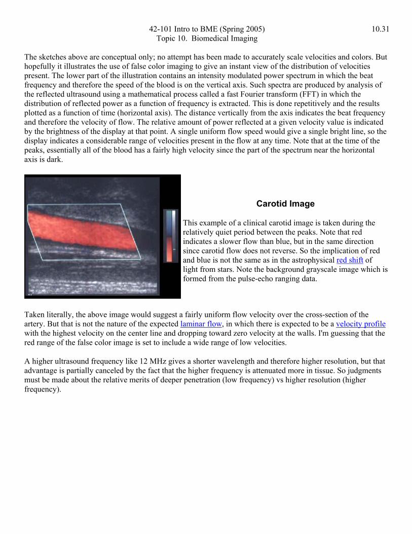
42-101 Intro to BME (Spring 2005) 10.31 Topic 10. Biomedical Imaging The sketches above are conceptual only; no attempt has been made to accurately scale velocities and colors. But hopefully it illustrates the use of false color imaging to give an instant view of the distribution of velocities present. The lower part of the illustration contains an intensity modulated power spectrum in which the beat frequency and therefore the speed of the blood is on the vertical axis. Such spectra are produced by analysis of the reflected ultrasound using a mathematical process called a fast Fourier transform (FFT) in which the distribution of reflected power as a function of frequency is extracted. This is done repetitively and the results plotted as a function of time (horizontal axis). The distance vertically from the axis indicates the beat frequency and therefore the velocity of flow. The relative amount of power reflected at a given velocity value is indicated by the brightness of the display at that point. A single uniform flow speed would give a single bright line, so the display indicates a considerable range of velocities present in the flow at any time. Note that at the time of the peaks, essentially all of the blood has a fairly high velocity since the part of the spectrum near the horizontal axis is dark.

Carotid Image

This example of a clinical carotid image is taken during the relatively quiet period between the peaks. Note that red indicates a slower flow than blue, but in the same direction since carotid flow does not reverse. So the implication of red and blue is not the same as in the astrophysical red shift of light from stars. Note the background grayscale image which is formed from the pulse-echo ranging data.

Taken literally, the above image would suggest a fairly uniform flow velocity over the cross-section of the artery. But that is not the nature of the expected laminar flow, in which there is expected to be a velocity profile with the highest velocity on the center line and dropping toward zero velocity at the walls. I'm guessing that the red range of the false color image is set to include a wide range of low velocities.

A higher ultrasound frequency like 12 MHz gives a shorter wavelength and therefore higher resolution, but that advantage is partially canceled by the fact that the higher frequency is attenuated more in tissue. So judgments must be made about the relative merits of deeper penetration (low frequency) vs higher resolution (higher frequency).


Magnetic Resonance Imaging – a tomographic technique that usesnon-ionizing radiation (radio frequency waves) Magnetic resonance imaging depends on immersing the body in a steady, strong magnetic field, commonly up to 1.5 Tesla (i.e. 15,000 Gauss for reference, the earth's magnetic field is about 0.5 Gauss). Some modern "whole-body" (i.e. apertures wide enough to accept a person's thorax) machines now operate at 4 or more Tesla. Hydrogen atoms, pervasive in the water which makes up about 70% of the body's mass, have a dipole property by virtue of their characteristic spins. These spinning atoms, influenced by the permeating magnetic field, precess like a top and a slight majority of hydrogen atoms precess in alignment with the dominant magnetic field.

Subjecting the body tissues to an additional magnetic field gradient to prepare a specific tissue slice of the body for imaging while adding a precisely tuned radio frequency pulse permits these specially prepared hydrogen atoms to absorb this radiation in a resonant fashion. Hydrogen atoms, by virtue of their surrounding magnetic environment and their excited state, alter their net magnetic axis direction temporarily. This excited state rapidly decays to a lower energy state while emitting its own unique radio frequency signal which can be detected by an external radio-frequency coil. From these signals there are mathematical methods for calculating images that produce tissue-related images. The relative brightness of individual points in the magnetic resonance imaging tomographic slice of the body provides information not only on the relative hydrogen content of that volume element (voxel), but also a unique signature of the local molecular and magnetic environment unique to the group of hydrogen atoms in specific molecular and local magnetic environments.

Special pulse-echo sequences permit high level signals to be detected from flowing blood, therefore images can be created of the vasculature and it's blood velocity characteristics.

So-called "functional MRI" detect differences oxygen-saturated and de-saturated blood. Thus brain processes of "thought" such as vision, motor control and speech can be detected (though at low spatial resolution) by virtue of their local oxygen consumption when activated.


http://info.med.yale.edu/intmed/cardio/imaging/techniques/mri_diagram/index.html

42-101 Intro to BME (Spring 2005) 10.35 Topic 10. Biomedical Imaging Magnetic Resonance Imaging and Spectroscopy – how it works http://www.erads.com/mrimod.htm http://www.cis.rit.edu/htbooks/mri/inside.htm The simple nucleus of the hydrogen atom consists of one proton, and no neutrons. The hydrogen atom has a positive charge and an atomic number of 1 due to the presence of only one proton in its nucleus. For the purposes of MR, the hydrogen atom is referred to as a proton. The abundance of the hydrogen atoms in the human body, and the large magnetic moment (discussed below) created by the single proton in the nucleus of the atom, make hydrogen atoms extremely sensitive to magnetic resonance. Based on these facts, we will concentrate on the hydrogen atom for the duration of this section. Hydrogen has the simplest atomic structure compared to all other elements.. Approximately 70% of the body is made up of water which contains two hydrogen atoms and one oxygen atom. It is the hydrogen atoms that are focused on to produce an MR image.

Spin

The moving (spinning) hydrogen protons create a magnetic field, and thus perform as a tiny magnet with a north and a south pole. Since there are two magnetic poles, the protons are referred to magnet dipoles. Based on the laws of electromagnetism, any electrically charged particle which moves creates a magnetic field called a magnetic moment. This is the property that allows hydrogen protons to behave predictably within an external magnetic field. The motion or the "spin" of the hydrogen atoms can be described as a random combination of the spinning of a top, the spin of a bowling ball and the rotation of the earth around its axis. Understanding the magnetic moment of the hydrogen protons, will lead to an understanding of the alignment of the protons within a magnet.

Spinning Proton No magnetic field present Magnetic field present


Spin is a fundamental property of nature like electrical charge or mass. Spin comes in multiples of 1/2 and can be + or -. Protons, electrons, and neutrons possess spin. Individual unpaired electrons, protons, and neutrons each possesses a spin of 1/2.

In the deuterium atom ( 2H ), with one unpaired electron, one unpaired proton, and one unpaired neutron, the total electronic spin = 1/2 and the total nuclear spin = 1.

Two or more particles with spins having opposite signs can pair up to eliminate the observable manifestations of spin. An example is helium. In nuclear magnetic resonance, it is unpaired nuclear spins that are of importance.

Other Nuclei with Spin

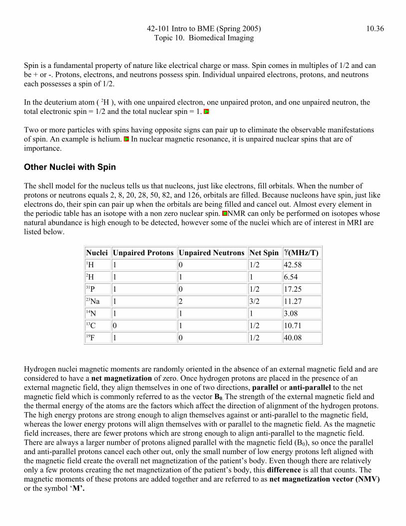
The shell model for the nucleus tells us that nucleons, just like electrons, fill orbitals. When the number of protons or neutrons equals 2, 8, 20, 28, 50, 82, and 126, orbitals are filled. Because nucleons have spin, just like electrons do, their spin can pair up when the orbitals are being filled and cancel out. Almost every element in the periodic table has an isotope with a non zero nuclear spin. NMR can only be performed on isotopes whose natural abundance is high enough to be detected, however some of the nuclei which are of interest in MRI are listed below.

Nuclei Unpaired Protons Unpaired Neutrons Net Spin (MHz/T) 1H 1 0 1/2 42.58 2H 1 1 1 6.54 31P 1 0 1/2 17.25 23Na 1 2 3/2 11.27 14N 1 1 1 3.08 13C 0 1 1/2 10.71 19F 1 0 1/2 40.08

Hydrogen nuclei magnetic moments are randomly oriented in the absence of an external magnetic field and are considered to have a net magnetization of zero. Once hydrogen protons are placed in the presence of an external magnetic field, they align themselves in one of two directions, parallel or anti-parallel to the net magnetic field which is commonly referred to as the vector B0. The strength of the external magnetic field and the thermal energy of the atoms are the factors which affect the direction of alignment of the hydrogen protons. The high energy protons are strong enough to align themselves against or anti-parallel to the magnetic field, whereas the lower energy protons will align themselves with or parallel to the magnetic field. As the magnetic field increases, there are fewer protons which are strong enough to align anti-parallel to the magnetic field. There are always a larger number of protons aligned parallel with the magnetic field (B0), so once the parallel and anti-parallel protons cancel each other out, only the small number of low energy protons left aligned with the magnetic field create the overall net magnetization of the patient’s body. Even though there are relatively only a few protons creating the net magnetization of the patient’s body, this difference is all that counts. The magnetic moments of these protons are added together and are referred to as net magnetization vector (NMV) or the symbol ‘M’.

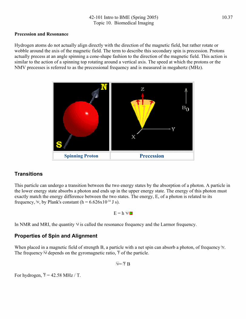
42-101 Intro to BME (Spring 2005) 10.37 Topic 10. Biomedical Imaging Precession and Resonance

Hydrogen atoms do not actually align directly with the direction of the magnetic field, but rather rotate or wobble around the axis of the magnetic field. The term to describe this secondary spin is precession. Protons actually precess at an angle spinning a cone-shape fashion to the direction of the magnetic field. This action is similar to the action of a spinning top rotating around a vertical axis. The speed at which the protons or the NMV precesses is referred to as the precessional frequency and is measured in megahertz (MHz).

Spinning Proton Precession

Transitions

This particle can undergo a transition between the two energy states by the absorption of a photon. A particle in the lower energy state absorbs a photon and ends up in the upper energy state. The energy of this photon must exactly match the energy difference between the two states. The energy, E, of a photon is related to its frequency, , by Plank's constant (h = 6.626x10-34 J s).

E = h

In NMR and MRI, the quantity is called the resonance frequency and the Larmor frequency.

Properties of Spin and Alignment

When placed in a magnetic field of strength B, a particle with a net spin can absorb a photon, of frequency . The frequency depends on the gyromagnetic ratio, of the particle.

= B

For hydrogen, = 42.58 MHz / T.

42-101 Intro to BME (Spring 2005) 10.38 Topic 10. Biomedical Imaging Energy Level Diagrams

The energy of the two spin states can be represented by an energy level diagram. We have seen that = B and E = h , therefore the energy of the photon needed to cause a transition between the two spin states is

E = h B

When the energy of the photon matches the energy difference between the two spin states an absorption of energy occurs.

In the NMR experiment, the frequency of the photon is in the radio frequency (RF) range. In NMR spectroscopy, is between 60 and 800 MHz for hydrogen nuclei. In clinical MRI, is typically between 15 and 80 MHz for hydrogen imaging.

CW NMR Experiment

The simplest NMR experiment is the continuous wave (CW) experiment. There are two ways of performing this experiment. In the first, a constant frequency, which is continuously on, probes the energy levels while the magnetic field is varied. The energy of this frequency is represented by the blue line in the energy level diagram.

The CW experiment can also be performed with a constant magnetic field and a frequency which is varied. The magnitude of the constant magnetic field is represented by the position of the vertical blue line in the energy level diagram.

Boltzmann Statistics

When a group of spins is placed in a magnetic field, each spin aligns in one of the two possible orientations.

At room temperature, the number of spins in the lower energy level, N+, slightly outnumbers the number in the upper level, N-. Boltzmann statistics tells us that

N-/N+ = e-E/kT.

E is the energy difference between the spin states; k is Boltzmann's constant, 1.3805x10-23 J/Kelvin; and T is the temperature in Kelvin.

As the temperature decreases, so does the ratio N-/N+. As the temperature increases, the ratio approaches one.

The signal in NMR spectroscopy results from the difference between the energy absorbed by the spins which make a transition from the lower energy state to the higher energy state, and the energy emitted by the spins which simultaneously make a transition from the higher energy state to the lower energy state. The signal is thus proportional to the population difference between the states. NMR is a rather sensitive spectroscopy since it is capable of detecting these very small population differences. It is the resonance, or exchange of energy at a specific frequency between the spins and the spectrometer, which gives NMR its sensitivity.

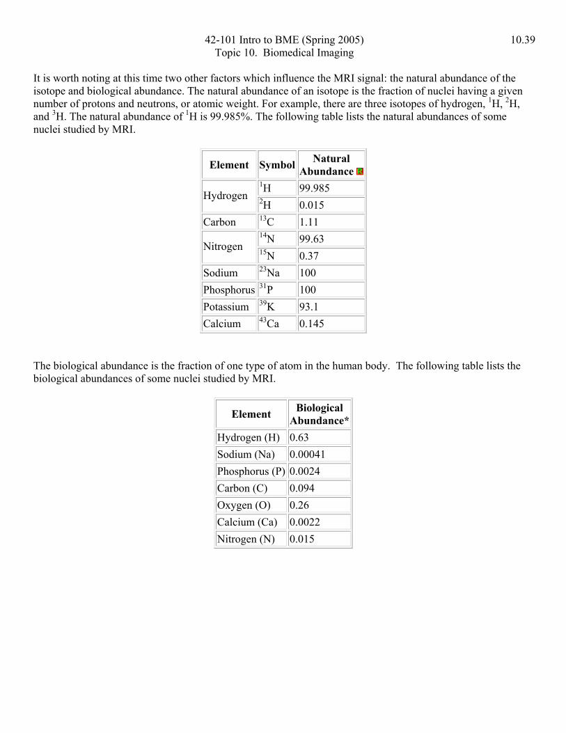
42-101 Intro to BME (Spring 2005) 10.39 Topic 10. Biomedical Imaging It is worth noting at this time two other factors which influence the MRI signal: the natural abundance of the isotope and biological abundance. The natural abundance of an isotope is the fraction of nuclei having a given number of protons and neutrons, or atomic weight. For example, there are three isotopes of hydrogen, 1H, 2H, and 3H. The natural abundance of 1H is 99.985%. The following table lists the natural abundances of some nuclei studied by MRI.

Element Symbol Natural Abundance

1H 99.985 Hydrogen 2H 0.015 Carbon 13C 1.11

14N 99.63 Nitrogen 15N 0.37 Sodium 23Na 100 Phosphorus 31P 100 Potassium 39K 93.1 Calcium 43Ca 0.145

The biological abundance is the fraction of one type of atom in the human body. The following table lists the biological abundances of some nuclei studied by MRI.

Element Biological Abundance*

Hydrogen (H) 0.63 Sodium (Na) 0.00041 Phosphorus (P) 0.0024 Carbon (C) 0.094 Oxygen (O) 0.26 Calcium (Ca) 0.0022 Nitrogen (N) 0.015

42-101 Intro to BME (Spring 2005) 10.40 Topic 10. Biomedical Imaging The Larmor Frequency

Tesla (T) or gauss is the measure of strength of the magnetic field. One Tesla is equivalent to 10,000 gauss, and is about 20,000 times stronger than the earth’s magnetic field. All protons precess at the same frequency within a magnetic field. The gyro-magnetic ratio of hydrogen is 42.57 MHz/Tesla. The gyro-magnetic ratio is different for each nucleus of different atoms. The frequency is determined by the gyro-magnetic ratio of atoms and the strength of the magnetic field. The Larmor equation is important because it is the frequency at which the nucleus will absorb energy. The absorption of that energy will cause the proton to alter its alignment. In MR imaging, the energy that is transferred is radio frequency waves (RF) and ranges from 1-100 MHz. The Larmor equation governs the value of the precessional frequency, and is follows:

Precessional frequency (w O) = B0 x l

B0 = the magnetic field strength of the magnet

l = the gyro-magnetic ratio.

At 1 T the precessional frequency of hydrogen is 42.57 MHz (1 T x 42.57 MHz)

At 1.5 T the precessional frequency of hydrogen is 42.57 MHz (1.5 T x 63.86 MHz)

The stronger the magnetic field, the higher the precessional frequency. If an RF pulse at the Larmor frequency is applied to the nucleus of an atom, the protons will alter their alignment from the direction of the main magnetic field to the direction opposite the main magnetic field. As the proton tries to realign with the main magnetic field, it will emit energy at the frequency of the Larmor frequency.

Resonance is referred to as the property of an atom to absorb energy only at the Larmor frequency. This is the basis of MR. An atom will only absorb external energy if that energy is delivered at precisely it’s resonant frequency. The energy must also be delivered at 90° to the net magnetic vector (NMV) and main magnetic field (B0). Otherwise, no energy will be absorbed, resonance will not have occurred and an image cannot be created. Excitation occurs when the proton absorbs the applied energy or resonates. As resonance occurs and the NMV moves out of alignment with the B0 to a pre-specified angle. The deflection of the magnetization or total angle created after the end of the RF pulse is referred to as the flip angle.

Longitudinal and Transverse Magnetization

The stronger the RF energy applied to the protons, the greater the angle of deflection for the magnetization. The two most common flip angles in MR are 90° and 180° . A 90° pulse will flip the magnetization into the x-y plane (Mxy). A 180° pulse will flip the magnetization through the x-y plane and into the opposite direction of B0.


Protons aligned with Z Axis After 90 degree pulse When a 90° pulse is applied and the protons are given enough energy to be flipped into the x-y plane, the net magnetization vector is now in the transverse plane. B0 or z-axis is now referred to as the longitudinal plane. The protons are now rotating in the transverse plane at the Larmor frequency. As well as flipping into the transverse plane, the protons also begin rotating in phase with each other. When resonance occurs, all the magnetic moments move into the same path or all flip the same number of degrees, and they all precess in phase with other.

With the net magnetization in the transverse plane (created with a 90° flip angle), and a receiver coil or antenna in the transverse plane, a voltage is induced within the receiver coil. This oscillating signal voltage over time is the MR signal. The magnitude of the signal is dependent on the magnetization present in the transverse plane. At the termination of the RF, the freely precessing protons in the transverse plane (Mxy) give up energy (RF) in order to try to realign with B0. As the transverse magnetization starts to decay due to the loss of phase coherence, the protons eventually realign with B0. This signal produced by the decay of transverse magnetization is called free induction decay (FID). The amplitude of the FID signal becomes smaller over time as net magnetization returns to equilibrium. Simultaneously, the longitudinal magnetization begins to recover and return to B0 to a state of equilibrium just as if nothing had occurred.

After the external RF signal is turned off, two phenomenons simultaneously occur.

• Longitudinal magnetization gradually increases and is called T1 recovery • Transverse magnetization gradually decreases and is called T2 decay

These phenomena are discussed in more detail below. In summary, atoms rotate randomly outside the presence of a magnetic field. When in the presence of an external magnetic field, the atoms align either with or opposed to the main magnetic field. The parallel and anti-parallel protons cancel each other out, leaving a relatively small number of protons aligned with the main magnetic field. As an RF signal is applied at the Larmor frequency, the individual protons resonate, or absorb the applied energy, and precess in phase. Depending on the strength of the applied energy, the protons will flip into the x-y plane (transverse magnetization), or exactly the opposite direction of the main magnetic field. The transverse magnetization induces a voltage in an antenna or receiver coil which will be eventually become the MR signal. As the RF is turned off, the protons dephase and lose their coherence as they try to realign with B0. Two phenomenons occur simultaneously. Transverse magnetization decreases (T2 decay), while longitudinal magnetization increases (T1 recovery).

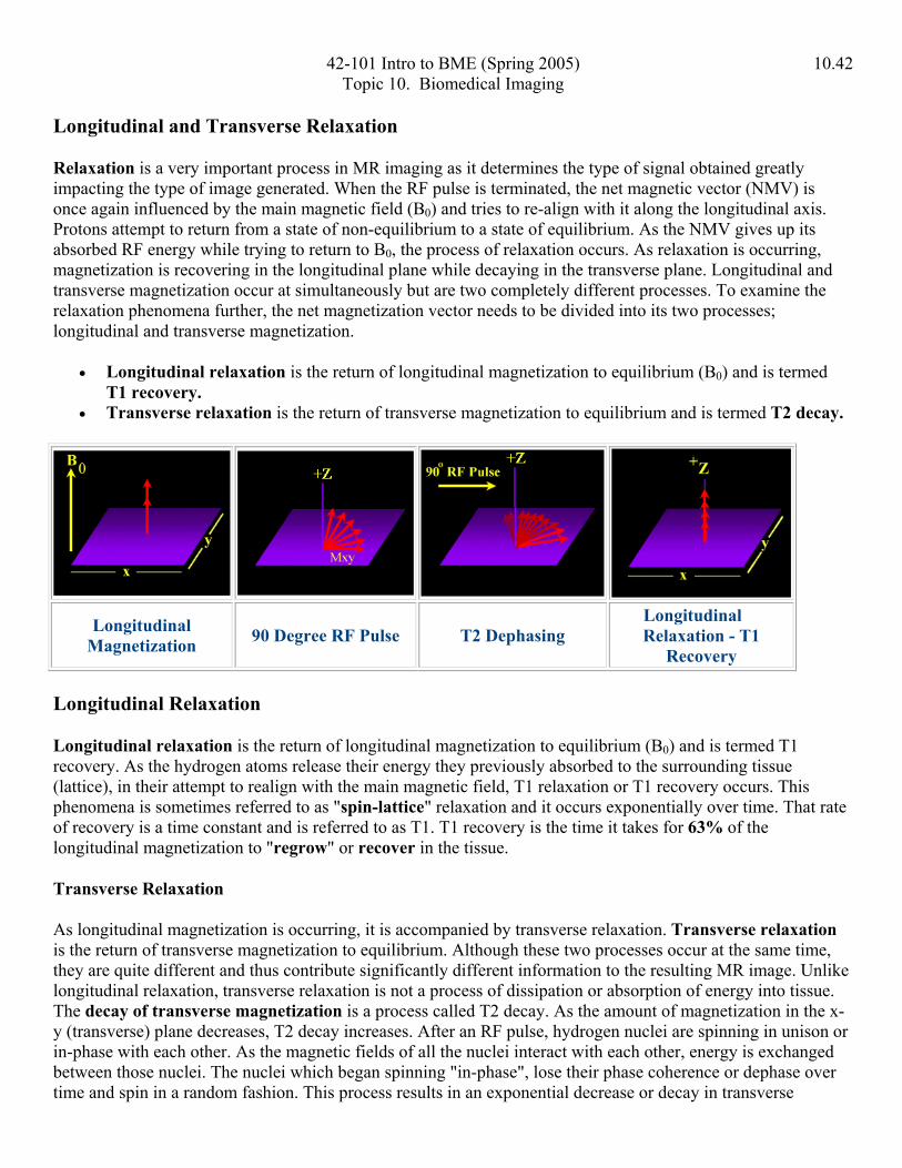
42-101 Intro to BME (Spring 2005) 10.42 Topic 10. Biomedical Imaging Longitudinal and Transverse Relaxation

Relaxation is a very important process in MR imaging as it determines the type of signal obtained greatly impacting the type of image generated. When the RF pulse is terminated, the net magnetic vector (NMV) is once again influenced by the main magnetic field (B0) and tries to re-align with it along the longitudinal axis. Protons attempt to return from a state of non-equilibrium to a state of equilibrium. As the NMV gives up its absorbed RF energy while trying to return to B0, the process of relaxation occurs. As relaxation is occurring, magnetization is recovering in the longitudinal plane while decaying in the transverse plane. Longitudinal and transverse magnetization occur at simultaneously but are two completely different processes. To examine the relaxation phenomena further, the net magnetization vector needs to be divided into its two processes; longitudinal and transverse magnetization.

• Longitudinal relaxation is the return of longitudinal magnetization to equilibrium (B0) and is termed T1 recovery.

• Transverse relaxation is the return of transverse magnetization to equilibrium and is termed T2 decay.

Longitudinal Magnetization 90 Degree RF Pulse T2 Dephasing

Longitudinal Relaxation - T1

Recovery Longitudinal Relaxation

Longitudinal relaxation is the return of longitudinal magnetization to equilibrium (B0) and is termed T1 recovery. As the hydrogen atoms release their energy they previously absorbed to the surrounding tissue (lattice), in their attempt to realign with the main magnetic field, T1 relaxation or T1 recovery occurs. This phenomena is sometimes referred to as "spin-lattice" relaxation and it occurs exponentially over time. That rate of recovery is a time constant and is referred to as T1. T1 recovery is the time it takes for 63% of the longitudinal magnetization to "regrow" or recover in the tissue.

Transverse Relaxation

As longitudinal magnetization is occurring, it is accompanied by transverse relaxation. Transverse relaxation is the return of transverse magnetization to equilibrium. Although these two processes occur at the same time, they are quite different and thus contribute significantly different information to the resulting MR image. Unlike longitudinal relaxation, transverse relaxation is not a process of dissipation or absorption of energy into tissue. The decay of transverse magnetization is a process called T2 decay. As the amount of magnetization in the x-y (transverse) plane decreases, T2 decay increases. After an RF pulse, hydrogen nuclei are spinning in unison or in-phase with each other. As the magnetic fields of all the nuclei interact with each other, energy is exchanged between those nuclei. The nuclei which began spinning "in-phase", lose their phase coherence or dephase over time and spin in a random fashion. This process results in an exponential decrease or decay in transverse

42-101 Intro to BME (Spring 2005) 10.43 Topic 10. Biomedical Imaging magnetization. Because T2 decay is the result of the exchange of energy between spinning hydrogen nuclei, it is referred to as "spin-spin" relaxation. As T2 decay occurs, the MR signal dies out. The rate of T2 decay is also expressed as a time constant. T2 decay occurs when the transverse magnetization has decreased to 37% of its initial value.

T1 Recovery Curve T2 Decay Curve Longitudinal relaxation is a regrowth or an increase in value, whereas transverse relaxation is a decrease or decay. Although these two processes occur together, T2 decay almost always occurs more rapidly than the regrowth of longitudinal magnetization.

Tissue Contrast

Due to the T1 and T2 relaxation properties, we can differentiate between various tissues in the body. As well as T1 and T2 contrast in tissues, proton density can also be measured. Proton density is measured by the number of protons per unit of tissue. Various tissues have different T1 and T2 values. These T1 and T2 values significantly influence the type of signal generated during MRI and thus contribute greatly to the MR image. Tissue contrast is affected by not only the T1 and T2 values of specific tissues, but the differences in the magnetic field strength, temperature changes and many other factors. It is not imperative that one memorize the absolute T1 and T2 values in different tissues, but being aware of the values may make a difference when the technologist is programming values for pulse sequences.

Fat Versus Water

Due to the slow molecular motion of fat nuclei, longitudinal relaxation occurs rather rapidly and longitudinal magnetization is regained quickly. The net magnetic vector realigns with B0 leading to a short T1 time for fat. Water is not as efficient as fat in T1 recovery due to the high mobility of the water molecules. Water nuclei do not give up their energy to the lattice (surrounding tissue) as quickly as fat, and therefore take longer to regain longitudinal magnetization resulting in a long T1 time.

As we know, T2 decay is dependent on the interaction of nuclei and the exchanging of energy with near by nuclei. Fat has a very efficient energy exchange and therefore has a relatively short T2. Water is less efficient than fat in the exchange of energy, and therefore has a long T2.


T1 and T2 CONSTANTS

T1 Constants at 1.5 T Controlled by TR

T2 Constants at 1.5 T Controlled by TE

Fat 85

Muscle 860 45

White matter 780 90

Gray matter 920 100

CSF 3000 1400 TR and TE are parameters controlled by the operator and are usually measured in milliseconds.

• TR stands for repetition time, or the elapsed time between successive RF excitation pulses. • TE stands for echo delay time, or the time interval between the RF pulse and the measurement of the

first echo.

The T1 constants above will indicate how quickly the spinning nuclei will emit their absorbed RF into the surrounding tissue. The T2 constants above will indicate how quickly the spinning nuclei will decay to 37% of the initial transverse magnetization.

T1, T2 and Proton Density Contrast

Fat has a shorter T1 time than water, therefore the fat vector will realign more quickly with the main magnetic field. It is obvious then that fat has a larger longitudinal component than water. After a 90° pulse, the longitudinal magnetization of both fat and water are flipped into the transverse plane. As previously mentioned, fat has a larger longitudinal component prior to an RF pulse, and it has a larger transverse component after an RF pulse. Due to the larger longitudinal and transverse magnetization, fat has a higher signal and will appear bright on a T1 contrast MR image. Conversely, water has less longitudinal magnetization prior to an RF pulse, therefore less transverse magnetization after an RF pulse yielding low signal appearing dark on a T1 contrast image. Images created with TR's and TE's to enhance T1 contrast are referred to as T1-weighted images.

The previously learned concepts of transverse magnetization apply for T2 contrast. Fat has a shorter T2 time than water and relaxes or decays more readily than water. Since the amount of transverse magnetization in fat is small, fat generates very little signal on a T2 contrast image and appears dark. Water has a very high T2 constant, therefore has very high T2 signal and thus appears bright on a T2 contrast image. Images created with TR's and TE's to enhance T2 contrast are referred to as T2-weighted images.

Proton density contrast is a quantitative summary of the number of protons per unit tissue. The higher the number of protons in a given unit of tissue, the greater the transverse component of magnetization, and the brighter the signal on the proton density contrast image. Conversely the lower the number of protons in a given unit of tissue, the less the transverse magnetization and the darker the signal on the proton density image.


T1 and T2 Weighting

Most all MR imaging will entail T1 and T2-weighted images among many other types of imaging. T1 and T2 images are the most common contrasts obtained in MRI. T1-weighted images are obtained to compare the T1 differences in tissues or to compare the relaxation rates of the tissue being examined. T2-weighted images are obtained to compare the T2 contrast in tissues and compare the transverse relaxation rates. Parameters are manipulated by the user to obtain the type of image contrast desired.

RF SIGNAL INTENSITIES IN TISSUE

High-Intensity Signal Low-Intensity Signal

Short T1 Long T1

Long T2 Short T2

High proton density low proton density

As previously stated, TR will control the T1-weighting of an MR image with a short TR maximizing T1-weighting and a long TR maximizing proton density-weighting

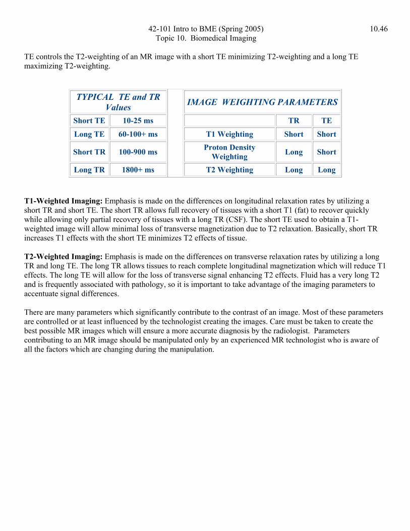
42-101 Intro to BME (Spring 2005) 10.46 Topic 10. Biomedical Imaging TE controls the T2-weighting of an MR image with a short TE minimizing T2-weighting and a long TE maximizing T2-weighting.

TYPICAL TE and TR

Values IMAGE WEIGHTING PARAMETERS

Short TE 10-25 ms TR TE

Long TE 60-100+ ms T1 Weighting Short Short

Short TR 100-900 ms Proton Density Weighting Long Short

Long TR 1800+ ms T2 Weighting Long Long T1-Weighted Imaging: Emphasis is made on the differences on longitudinal relaxation rates by utilizing a short TR and short TE. The short TR allows full recovery of tissues with a short T1 (fat) to recover quickly while allowing only partial recovery of tissues with a long TR (CSF). The short TE used to obtain a T1-weighted image will allow minimal loss of transverse magnetization due to T2 relaxation. Basically, short TR increases T1 effects with the short TE minimizes T2 effects of tissue.

T2-Weighted Imaging: Emphasis is made on the differences on transverse relaxation rates by utilizing a long TR and long TE. The long TR allows tissues to reach complete longitudinal magnetization which will reduce T1 effects. The long TE will allow for the loss of transverse signal enhancing T2 effects. Fluid has a very long T2 and is frequently associated with pathology, so it is important to take advantage of the imaging parameters to accentuate signal differences.

There are many parameters which significantly contribute to the contrast of an image. Most of these parameters are controlled or at least influenced by the technologist creating the images. Care must be taken to create the best possible MR images which will ensure a more accurate diagnosis by the radiologist. Parameters contributing to an MR image should be manipulated only by an experienced MR technologist who is aware of all the factors which are changing during the manipulation.

42-101 Intro to BME (Spring 2005) 10.47 Topic 10. Biomedical Imaging Handling and Processing Image Data http://www-ipg.umds.ac.uk/mpss99/Lecture_Notes/intro_html/imaging_intro.html

Spatial resolution

Fourier analysis

An extremely useful tool for simplifying a complicated function, is to break it down into a linear combination of sinusoidal components. This approach is known as Fourier Analysis. Joseph Fourier originally used it to study distribution of heat in a solids. It is equally applicable to the study of the distribution of brightness in a medical image.

Each sinusoidal component has characteristic frequency and phase. Because the image contains spatial information,the frequency components are called spatial frequency , and have units (1/length), eg: mm -1

An image can, therefore, be thought of as a sum of different spatial frequency component.

• Low spatial frequency is about slowly changing parts of image. • High spatial frequency components provide information about fast changing

parts of image ie: the fine detail.

The resolution of an image is a measure of how much fine detail can be seen, ie: the highest spatial frequency in the image. It is often measured using a pattern of parallel lines of different separation, measured in line-pairs per millimetre. The smallest separation (highest line-pair per mm) that can be correctly seen as two lines gives the resolution.

The resolution of medical images is normally different in different directions (anisotropic) and often varies with position in the image (heterogeneous).


Modulation transfer function

Real imaging systems are not equally sensitive to all spatial frequencies. • The modulation transfer function describes this relationship • The modulation transfer function is simply the Fourier Transform of the

impulse response function (the appearance in an image of an object that is a point).

More formally:

If f(x) is the object and F(k) is the object in the spatial frequency domain.

The imaging process involves convolving the object with the impulse response function of the imaging system g , giving .

The equivalent operation in the Fourier (k-space) domain is multiplication of the objects spectrum by the G , the modulation transfer function, ie:

Contrast Resolution

Adjacent image features that have very different brightness are said to have high contrast . Contrast, C , between features x and y of brightness B x and B y is defined as:

The contrast resolution of an imaging system is the lowest value of C that can be discerned. This depends on the noise.


Digital Images

Medical images stored on a computer are discrete .

They are stored as an array of numbers each corresonding to a different position in the patient.

In two dimensions (2D) the elements in the array are called picture elements (pixels).

• Pixels are not necessarily square, but all pixels have the same dimensions.

In three dimensions (3D), the pixel becomes the volume element (Voxel)

• The third dimension can be spatial as above, (eg: MR or CT) or temporal (eg: fluoroscopy).

42-101 Intro to BME (Spring 2005) 10.50 Topic 10. Biomedical Imaging We can have a fourth dimension, most commonly a 3D image volume acquired over time.

Dimensions of images

• An image has dimensions in pixels or voxels (eg: 256x256x124 for a typical MR image volume)

• Each pixel or voxel has spatial dimensions (eg: 0.8mm x 0.9 mm x 2mm). • Image data is normally stored as a list of raw values, with a separate header

(at the beginning of the file, or in a separate file) to describe the image. • The third dimension is often treated differently from the first two. A 3D

image is commonly treated as a sequence of 2D images.

Spatial Sampling

• The process of forming a discrete image from a continuous object is called sampling .

• The gap between the centre of adjacent samples in a given direction is the sampling interval . The sampling interval is often anisotropic.

• sampling interval in the through-slice direction in tomographic images is often larger than in the slice plane.

• The sampling can be at regular intervals,or irregular intervals. • normally (but not always) regular in a 2D image, or in the slice plane of

a multi-slice image. • sometimes irregular in the through-slice direction


Fourier Transforms (FT)

• The FT is mathematical tool to alter a difficult problem into one that can be solved.

• The FT converts a function (eg: an image) from one domain to another. For images, it converts between the spatial domain (the axes are distances, x ) and the spatial frequency domain (the axes are 1/distance, k ), i = (an imaginary number) .

Convolution

• the action of a sensor (eg: a camera) when it takes a weighted mean of a physical quantity (eg: light arriving at the camera) over a narrow range of some variable (distance).

• A convolution in one domain reduces to multiplication in the inverse domain.

Digital images are discrete:

• If an image is correctly sampled, it is possible to recover image values between the sample points with full accuracy.

• The sampling interval must not exceed the semiperiod of a sinusoid of the maximum frequency present in the function being sampled.


Sampling theorem

The minimum sampling frequency (the Nyquist frequency) must be twice the the highest frequency in the original sample for the sampled data to accurately represent the original data.

fNyquist = 2fmax

Another way of looking at sampling…

A function whose Fourier transform is zero for frequencies |k| greater than a cut off frequency kc is fully specified by values spaced at equal intervals not exceeding 1/2 kc-1 save for any harmonic terms with zeros at the sampling points . - Whittaker - Shannon

sampling theorem

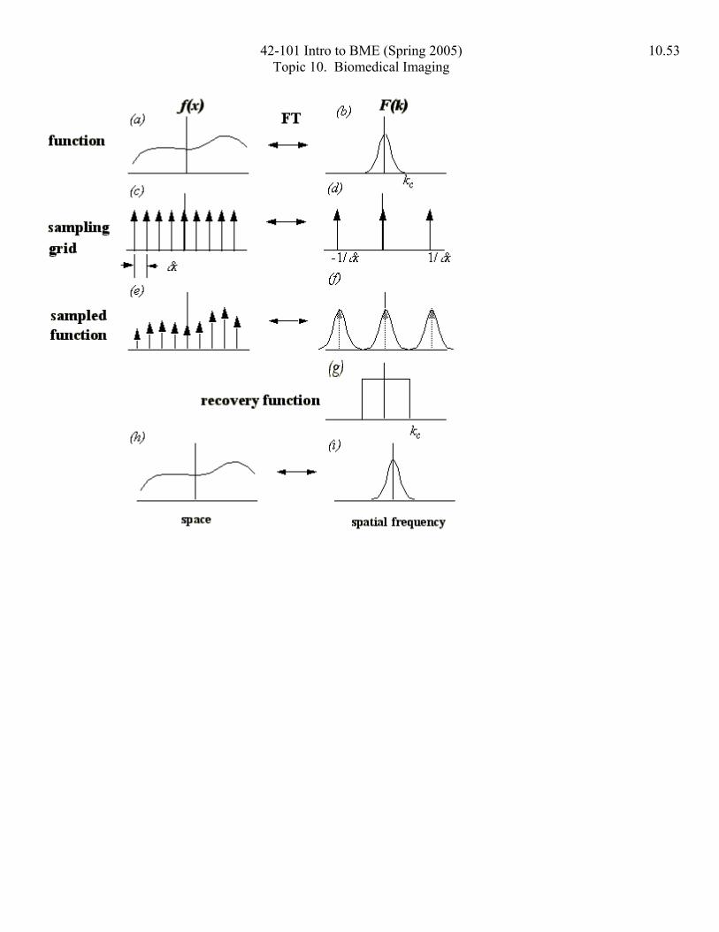
It can be helpful to consider the sampling theorem using the following diagram, which is one-dimensional for simplicity. The left column is in the spatial domain, and the right column the spatial-frequency domain, or k-space.

• The continuous function f(x) we wish to sample is is shown in panel (a). It has the continuous spectrum F(k) shown in (b).

• The function f(x) being sampled is band limited, as can be seen by the restricted range of spatial frequencies in the spectrum (maximum spatial frequency k c ).

• The function is sampled by multiplying it by the continuous "comb" of delta functions (c). The separation of the spikes on the comb is dx . The sampled function is shown in (e).

• The Fourier transform of the sampling function is shown in (c). • The k-space equivalent of multiplication in the image domain is

convolution. The sampling operation is, therefore, equivalent to convolution of the F(x) with the Fourier transform of the sampling function. The result is shown in (f).

• dx needs to be small enough that the tails of the spectrum F(k) do not overlap in panel (f), ie: (satisfied in this case).


Aliasing

An alternative view of the sampling theorem: all frequencies of the form

[f – kfsample] where k is an integer look the same.

If the sampling interval is too large ( ), then frequencies that are too high to be sampled correctly are aliased to lower frequencies. This phenomenon is very important in medical imaging. Remembering that an image can be decomposed into a sum of sinusoidal components, we can illustrate aliasing by considering a single continuous sinusoid. The thick black line is the signal. The sampling function is the series of rounded-spikes. The sampling interval is more than a half period of the sinusoid, and the resulting aliased signal is shown as the black dotted line.


Interpolation

If the object is correctly sampled, then intermediate values betweem sample points can be calculated. From the sampling theorem diagram above, it is clear that (b) can be recovered from (f) by multiplying (f) by the top-hat function (g). The equivalent operation in the spatial domain is convolution of (e) with the FT of (g), which is a

sinc ( ) function. The correct interpolation function is, therefore, the sinc function.

Note: • In practical terms, a sinc function has infinite extent, so cannot be used. • Where speed is the priority, nearest neighbour, or linear interpolation is

used. • Where accurate interpolation is important, higher order interpolants are used

eg: cubic, approximation to sinc function. • Interpolation errors increase with spatial frequency (largest for sharp edges

or points, smallest for uniform parts of image). • Interpolation is essential when images are translated by fractions of voxels

or rotated, eg: to align two images acquired at different times. • Sinc interpolation is correct for uniformly sampled data. To interpolate

irregularly sampled data onto a regular grid, inverse sinc interpolation is required.


k -Space

k -Space is the term given to the inverse spatial domain. The units are 1/distance. k x is 1/ x and k y is 1/ y .

Historical note : The terminology originally comes from solid state physics, where it is common to describe waves incident on a crystal lattice using the wave vector k, and to carry out calculations in the reciprocal lattice or k -space. We have not used the solid state notation here.

MRI is the imaging modality for which it is most important to consider k -Space.


Properties of K Space

• Every point in k-space effects the entire image • The centre of k -Space (usually the point just up and right from the centre) is

0 frequency (DC). • The edges of k -Space correspond to high spatial frequencies • D kx and D ky determine the pixel separation ∆ x and ∆ y: Increasing the

number of points in k -space for a given field of view increases the maximum spatial frequency content of the image, and hence the image resolution

• ∆ k x and ∆ k y determine the image field of view D x and D y .: increasing the separation of points in k -space while maintaining the number of points decreases the field of view of the image


Contrast of digital images

Just as a digital image is sampled at discrete positions in space, so the image brightness can take discrete values. The number of discrete values needed to correctly store a digital image depends on the ratio between brightess ranges required and the spread of the noise.

For example, if the brightness range to be stored is 1000 times the standard deviation of the noise, then 1000 discrete brightness levels are needed. The number of bits needed to store 1000 brightness values is 10 (this would, in fact store values 0 - 1023). This corresponds to saying that the least significant bit samples only noise.

• Pixel or voxel values are normally stored at byte boundaries, or perhaps nibble boundaries (1 byte = 2 nibble)

• Many medical images need between 10 and 12 bits per pixel or per voxel. Display

The digital image is displayed onto a computer monitor (CRT or LCD).

Displaying brightness values

• Displays normally support 8 bits of brightness (0-255) • The image brightness values have to be mapped onto the range of

brightnesses supported by the screen. This is often called "windowing". • The minimum and maximum image brightness values to be displayed are

chosen, as is the intensity transformation (eg: linear or logarithmic).

Displaying pixel values

• Displays typically have 1000+ pixels in each direction • The image pixels or voxels have to be re-sampled for display

• image pixels or voxels may have non-uniform aspect ratio, but screens have square pixels.


• interpolation : if the portion of the image to be viewed has fewer pixels than the part of the display being used, then intermediate image values need to be interpolated.

• sub-sampling . If the portion of the image to be viewed has more pixels than the part of the display being used, then the image is subsampled, eg: by displaying alternate pixels, or by re-sampling using a Gaussian kernel that does local averaging.

Simple image segmentation

Motivation

• Measuring volumes (eg: MS lesions, hippocampus) • Quantifying abnormalities eg: percentage stenosis • Visualisation of structures eg: tumours • Automatic identification of lesions eg: computerised mamogram reporting • Measure "shape" of structures, eg: to characterize abnormality.

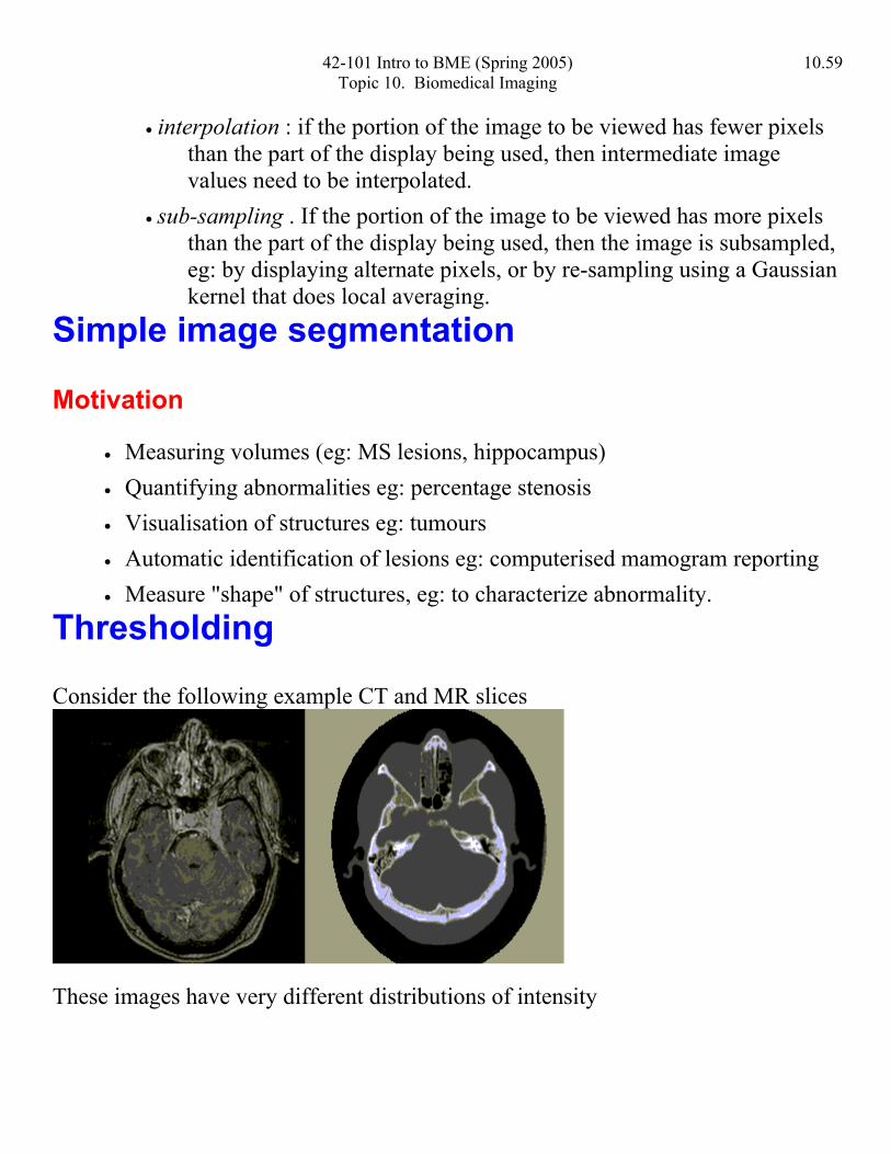
Thresholding

Consider the following example CT and MR slices

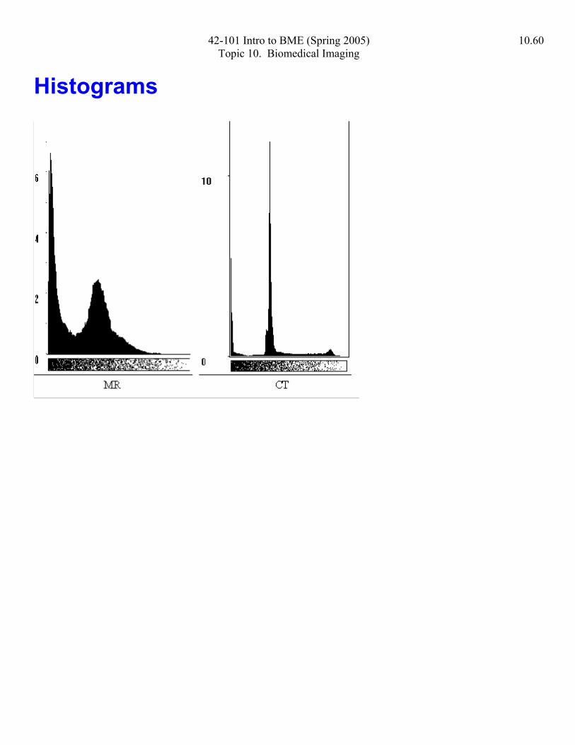
These images have very different distributions of intensity


Histograms


Thresholded results


Region Growing

Consider an image with two separate structures with similar intensities, eg: the brain and scalp in this image below.

• Thresholding segments the brain + scalp (approximately) • Region growing can be used to segment a single connected region, eg:

brain. • Region growing needs: UPPER THRESHOLD, LOWER THRESHOLD,

SEED POINT. • Define connectivity (eg: 4 connect or 8 connect in 2D) • Start at seed point, and check each neighbour in turn, to see if it is within

valid intensity range. If yes, add to list of valid pixels. • Choose next valid pixel, and repeat. • Small connections between regions cause problems.

types of images - carnegie mellon university// ... mechanism of that attenuation is ionization of...

Documents